A U-Shaped Convolution-Aided Transformer with Double Attention for Hyperspectral Image Classification

Abstract

Convolutional neural networks (CNNs) and transformers have achieved great success in hyperspectral image (HSI) classification. However, CNNs are inefficient in establishing long-range dependencies, and transformers may overlook some local information. To overcome these limitations, we propose a U-shaped convolution-aided transformer (UCaT) that incorporates convolutions into a novel transformer architecture to aid classification. The group convolution is employed as parallel local descriptors to extract detailed features, and then the multi-head self-attention recalibrates these features in consistent groups, emphasizing informative features while maintaining the inherent spectral–spatial data structure. Specifically, three components are constructed using particular strategies. First, the spectral groupwise self-attention (spectral-GSA) component is developed for spectral attention, which selectively emphasizes diagnostic spectral features among neighboring bands and reduces the spectral dimension. Then, the spatial dual-scale convolution-aided self-attention (spatial-DCSA) encoder and spatial convolution-aided cross-attention (spatial-CCA) decoder form a U-shaped architecture for per-pixel classifications over HSI patches, where the encoder utilizes a dual-scale strategy to explore information in different scales and the decoder adopts the cross-attention for information fusion. Experimental results on three datasets demonstrate that the proposed UCaT outperforms the competitors. Additionally, a visual explanation of the UCaT is given, showing its ability to build global interactions and capture pixel-level dependencies.

1. Introduction

Hyperspectral images (HSIs) are data cubes captured by hyperspectral sensors, which simultaneously reveal 2-D spatial and 1-D spectral information about land cover substances [1]. What distinguishes HSIs from panchromatic and multispectral images is that their pixels record the distinctive spectral signatures using hundreds of nearly continuous spectral bands [2,3,4]. The high-resolution spectral response curves reflect detailed characteristics of land cover substances [5]. Consequently, hyperspectral image (HSI) classification, defined as “assigning a certain category to each pixel [6]”, has become a fundamental but crucial aspect of remote sensing applications. However, abundant spectral information could also be redundant due to some highly correlated spectral bands [7,8,9]. Moreover, there are some other hindrances to HSI classification. The spectral variability [10,11] and the lack of labeled training samples, for example, would negatively affect the HSI feature extraction and make the classification more challenging. These adverse effects have heightened the need for advanced feature extraction networks.

Over recent years, deep learning has emerged as the most preferable approach to extracting informative features thanks to its ability in feature representation. Typical deep learning networks, such as stacked autoencoders (SAEs) [12,13], recurrent neural networks (RNNs) [14,15,16], convolutional neural networks (CNNs), and transformers, have been widely used in HSI classification. Among them, CNN- and transformer-based networks, which excel at local perception and global interaction, respectively, have established their superiority in HSI classification.

In general, there are three types of HSI classification methods based on different ways of feature extraction [17]: spectral-feature networks, spatial-feature networks, and spectral–spatial-feature networks. Accordingly, CNN-based networks could also be intuitively divided into 1-D CNNs [18,19], 2-D CNNs [20], and 3-D CNNs [21]. Facing the same problem as SAEs and RNNs, 1-D CNNs only exploit spectral features, whereas spatial features are somewhat weakened [22,23]. However, 2-D CNNs are inclined to assemble only spatial information. Nevertheless, previous studies have indicated that the individual spectral or spatial features may not achieve a satisfactory performance [24]. Spectral features provide the most revealing insight into land cover substances, while spatial features could add some complementary information, and an integration would achieve better classification performance than the individual ones. Therefore, 3-D CNNs were employed to extract features in spectral and spatial dimensions jointly. For example, Zhong et al. [25] proposed a spectral–spatial residual network (SSRN) that adopts 3-D CNN as the basic element to extract spectral–spatial features, achieving impressive performance. In fact, 3-D CNNs are just the most direct ways of spectral–spatial feature extraction, and there are some other approaches. Zhao et al. [26] developed two kinds of 1-D CNNs to extract spectral and spatial features and then fused these features. Zhang et al. [27] combined 1-D CNN with 2-D CNN to exploit spectral–spatial features efficiently. Roy et al. [28] proposed a hybrid spectral CNN (HybridSN) that combines 3-D CNN with 2-D CNN and thus reduces the computation overload. Huang et al. [29] used a 3-D CNN and a pyramid squeeze-and-excitation attention module to extract spectral–spatial features jointly.

Based on the multi-head self-attention (MSA) mechanism [30], transformers have become a dominant paradigm of natural language processing (NLP) and have made significant progress in computer vision (CV) tasks as well. In 2020, vision transformer (ViT) [31] pioneered the use of transformers for CV tasks, which provides an efficient method for modeling long-range dependencies and establishing global interactions. Then, many researchers committed to adapting ViT to HSI classification. Specifically, for the patches embedding layer, there are three different perspectives of tokenization: spectral, spatial, and spectral–spatial perspectives. The spatial–spectral transformer (SST) [32] and spectral former [33] treated HSIs as spectral sequential data for tokenization. The main difference is that the former utilized a VGG-like architecture to tokenize each band separately, while the latter designed a groupwise spectral embedding layer to tokenize overlapped bands. HSI-BERT [34], on the other hand, concentrated on modeling spatial dependencies among pixels in a spatial perspective. From a spectral–spatial perspective, Sun et al. [1] developed a model called the spectral–spatial feature tokenization transformer (SSFTT), which extracts spectral–spatial features and then makes samples more separable using a Gaussian-weighted feature tokenizer. As for the transformer encoder layer, many improvements have also been made in order to facilitate feature representation. For example, Liang et al. [35] developed a dual multi-head contextual self-attention (DMuCA) network that decouples spatial and spectral contextual attention into two subblocks, capturing rich contextual dependencies from both the spatial and spectral domains.

Albeit the exciting progress the aforementioned methods have made, there are still some imperfections:

(1)

CNNs are good at local perception and extracting low-level features. However, they treat all features equally without considering different significances. Moreover, capturing global contextual information and establishing long-range dependencies can be inefficiently limited by their inherent structure [36].

(2)

Transformers are good at global interaction and capturing salient features. However, they often manifest difficulty in local perception [37,38], which is nevertheless critical to the collection of refined information. Furthermore, transformers usually have a considerable demand for training data [39], yet annotated HSI data are mostly inadequate. Moreover, the internal spectral–spatial data structure can be damaged in the transformer architecture, which deteriorates the classification performance.

(3)

Most of these CNN- and transformer-based networks follow a patch-wise classification framework; that is, each pixel with its adjacent pixels can form a coherent whole that is labeled as the category of the center pixel [40,41]. This framework is grounded on the spatial homogeneity assumption that the adjacent pixels will share the same land cover category with their center pixel. However, the assumption is not always tenable because the cropped patch is too complicated in spatial distribution to be roughly represented by its center pixel.

To alleviate the above problems, we propose a U-shaped convolution-aided transformer (UCaT) that embeds group convolutions into a U-shaped transformer architecture to aid the per-pixel identifications over cropped HSI patches, making full use of both the advantages of CNNs and transformers. Hence, it is the classification map, not one label, that is generated for a patch. Accordingly, the spatial homogeneity assumption we mentioned in the third problem can be a guide, not a hard constraint. And in response to the limitations of CNNs and transformers, we introduce such reasonable inductive bias of CNNs as locality to the transformer. Specifically, by replacing linear projection with group convolutional projection, the UCaT is dominated by a transformer to focus on salient features and capture global dependencies. And it cooperates with convolutions for local perception and lowering the demand for training data. Based on this, three components are constructed using particular strategies. First, the spectral groupwise self-attention (spectral-GSA) component treats HSIs as sequential spectral data for extracting discriminative spectral features. Then, the spatial dual-scale convolution-aided self-attention (spatial-DCSA) encoder and the spatial convolution-aided cross-attention (spatial-CCA) decoder form a U-shaped architecture for building spatial attention, which effectively assembles local-global spatial information. Overall, the main contributions can be summarized as:

(1)

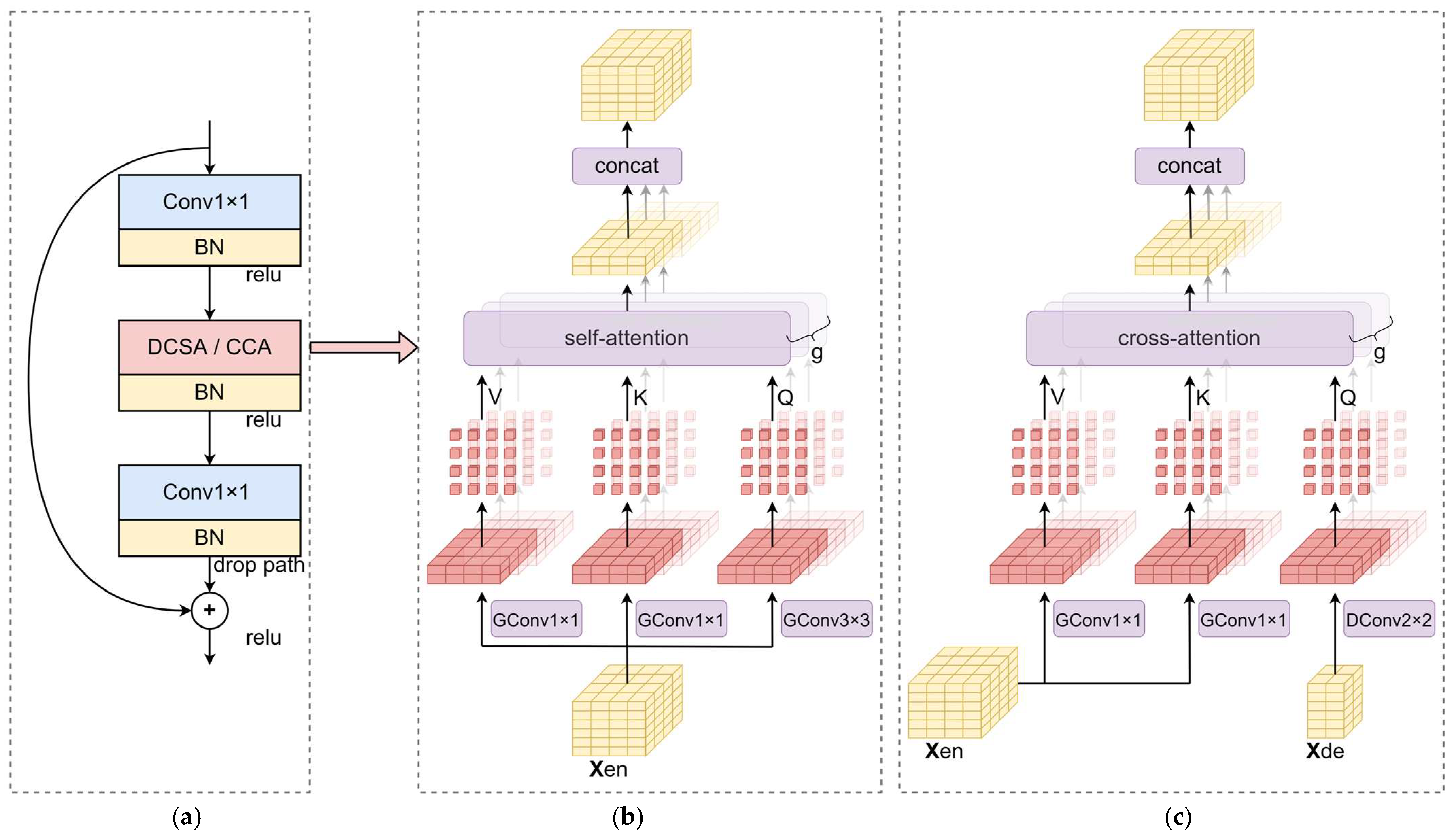
A UCaT network, which incorporates group convolutions into a novel transformer architecture, is proposed. The group convolution extracts detailed features locally, and then the MSA recalibrates the obtained features with a global field of vision in consistent groups. This combination takes full account of the characteristics of HSI data, emphasizing informative features while maintaining the inherent spectral–spatial data structure.

(2)

The spectral-GSA builds spectral attention and provides a new way of dimensionality reduction. It divides the spectral bands into small groups and builds spectral attention in groups, which possesses the ability to capture subtle spectral discrepancies. And a convolutional attention weight adjustment is constructed, which efficiently reduces the spectral dimension.

(3)

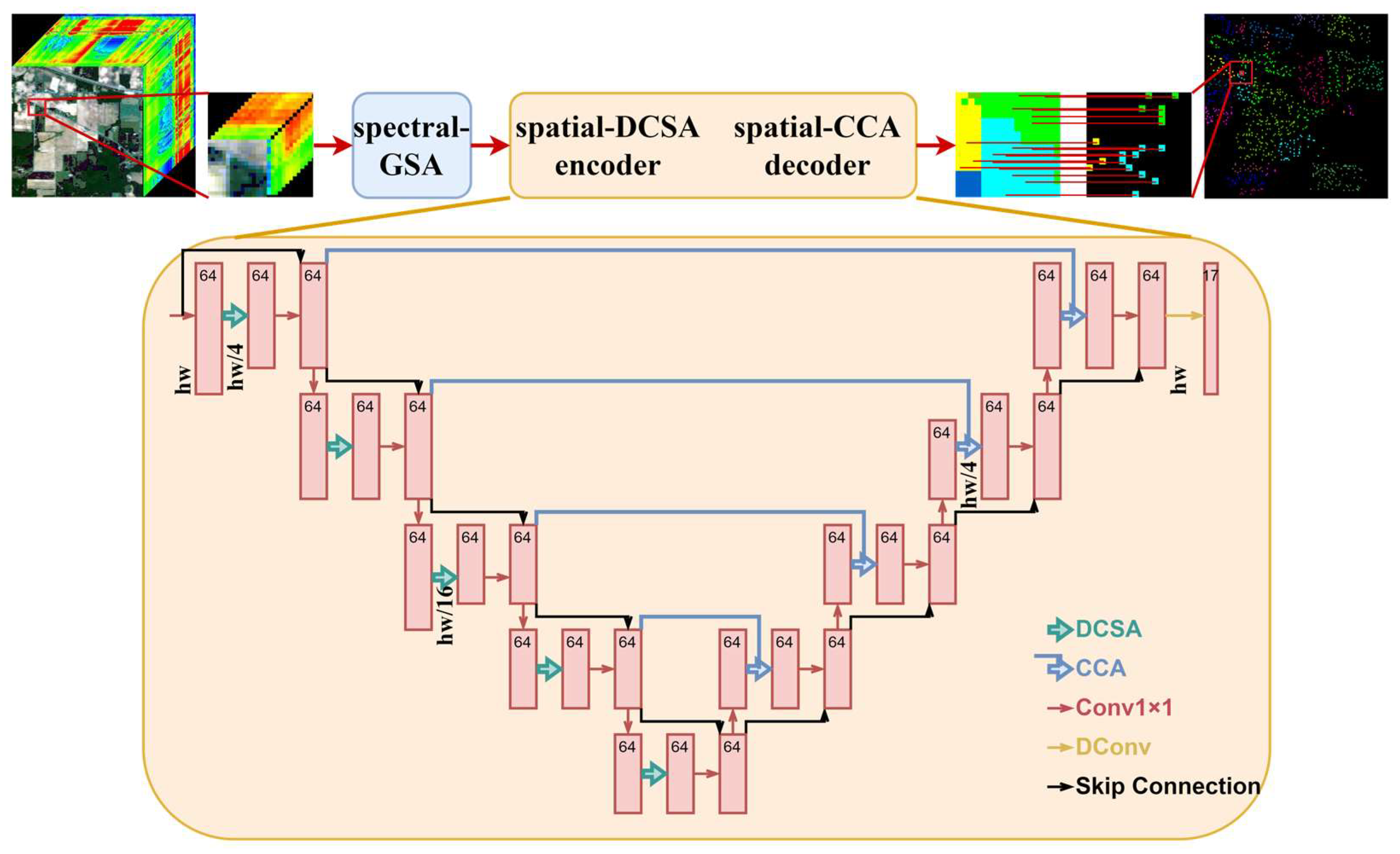
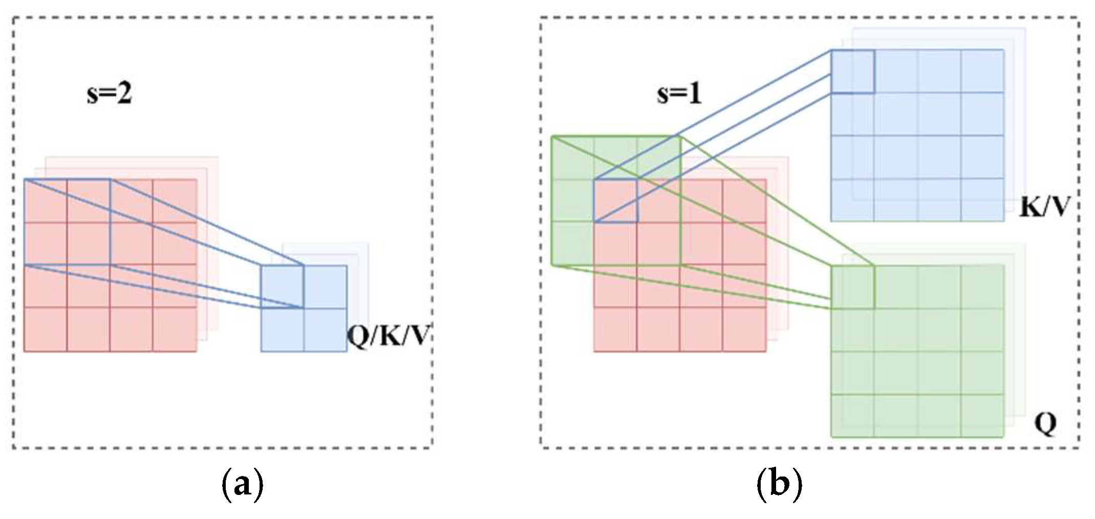
The spatial-DCSA encoder and the spatial-CCA decoder form a U-shaped architecture to assemble local-global spatial information, where a dual-scale strategy is employed to exploit information in different scales, and the cross-attention strategy is adopted to compensate high-level information with low-level information, which contributes to spatial feature representation.

(4)

The UCaT achieves better classification results and better interpretability. Extensive experiments demonstrate that the UCaT outperforms the CNN- and transformer-based state-of-the-art networks. A visual explanation shows that the UCaT can not only distinguish homogeneous areas to eliminate semantic ambiguity but also capture pixel-level spatial dependencies.

The remaining sections of this article are organized as follows. Section 2 revisits the related works, i.e., transformer-based networks and segmentation networks. Section 3 gives a brief introduction to the proposed network. Section 4 presents experimental details and classification results, and Section 5 visually explains the proposed network. Finally, Section 6 concludes this article.

2. Related Works

2.1. Transformer-Based Networks

As the basic part of transformers, MSA provides a new topology for feature extraction. As the name suggests, MSA is assembled of multiple self-attention blocks that selectively emphasize discriminative features. Specifically, given the input $X\in {ℝ}^{n\times d}$, where n is the number of sequences, d is the dimension of each sequence. X is initially linear mapped into Query $Q\in {ℝ}^{n\times d_k}$, Key $K\in {ℝ}^{n\times d_k}$, and Value $V\in {ℝ}^{n\times d_v}$, where d_k indicates the dimension of Q and K, and d_v indicates the dimension of V. The attention weight matrix $A\in {ℝ}^{n\times n}$ can then be calculated to measure the similarity between Q and K using the scaled dot-product. Then, the output can be obtained by assigning the matched attention weight to V. This calculation can be expressed as:

$$\mathrm{Attention}\left(Q,K,V\right)=\mathrm{softmax}\left(\frac{Q{K}^{\mathrm{T}}}{\sqrt{d_k}}\right)V$$

(1)

To further capture richer information from different subspaces, the self-attention blocks can be concatenated, and then a linear transformation is performed to integrate information from these self-attention blocks. This whole process is known as the MSA and can be formally described as:

$$\mathrm{MSA}\left(Q,K,V\right)=\mathrm{concat}\left({\mathrm{head}}_1,{\mathrm{head}}_2,\dots ,{\mathrm{head}}_h\right)W^O$$

(2)

where $W^O$ represents the trainable parameter matrix, h is the number of heads, and ${\mathrm{head}}_i=\mathrm{Attention}\left(Q_i,K_i,V_i\right)$.

In recent years, transformer-based networks have been broadly studied. Liu et al. [42] proposed a swin transformer that calculates MSA over non-overlapping local windows and enables cross-window interactions through the shifted windowing operation. Touvron et al. [39] established a data-efficient image transformer (DeiT) with a novel distillation procedure that uses a distillation token to reproduce teacher’s labels, performing well without a very large amount of training data. It has been further pointed out in their paper that CNNs could be better teachers than transformers, probably because the inductive bias of CNNs can be implicitly inherited through distillation. On the other hand, some research directly grafted CNNs to transformers and performed well, e.g., CvT [43], CeiT [38], LeViT [44], etc. Despite the great success the foregoing networks have achieved in CV tasks, there are still problems. For example, it is inappropriate to directly utilize the networks that are commonly designed for conventional RGB images for high-dimensional HSI images.

2.2. Segmentation Networks

To solve the aforementioned problem that the center pixels are insufficient to represent the categories of the whole patches, two main methods can be used. The first method is to distinguish the center pixels from others. The central attention network (CAN) [45] and cross-attention spectral–spatial network (CASSN) [46], for example, paid extra attention to the center pixels, outperforming the traditional patch-wise classification methods. Second, instead of assigning a certain category to a whole patch, segmentation networks make dense predictions for all pixels in a patch simultaneously, yielding a simpler yet more efficient network structure than the first method. UNet [47], significantly, is a classical segmentation network. It was designed based on an encoder-decoder framework. The encoder branch extracts hierarchical features with downsampling and channel expansion, while the decoder branch restores the resolutions of features by upsampling, and features from both branches can be combined using feature concatenation method. In this paper, we use the U-shaped encoder-decoder architecture of UNet and propose a new convolution-aided transformer for HSI classification.

3. Methodology

In this section, we will first give a brief introduction to the overall structure of the proposed UCaT and then describe its individual components.

3.1. Overview

The overall structure of the proposed UCaT is depicted in Figure 1. The classification flowchart inherits the work in [48], where a few modifications to the traditional patch-wise classification flowchart were made so that it can take classification maps as output. And we propose a UCaT network that makes dense identifications of cropped HSI patches. Thus, the spatial homogeneity assumption could also provide a soft spatial prior with the aim of avoiding the salt-and-pepper noise but not forcing the labels of a whole patch to be the label of its center pixel.

Let $H\in {ℝ}^{C\times H\times W}$ represent the original HSI data, where H, W, and C denote the spatial height, width, and the number of bands, respectively. And $Y\in {ℝ}^{N\times H\times W}$ indicates the ground truth of H, where N is the number of land cover categories (note that all the unlabeled pixels are subsumed into an additional category, i.e., 0). After removing all the unlabeled pixels, the remaining pixels can be randomly divided into training pixels and testing pixels. For each pixel p_i as one of the training pixels, the patch $X_i\in {ℝ}^{C\times h\times w}$ centered on p_i is cropped from H to set up the training set, where $h\times w$ indicates the cropped window size. And so does the ground truth map: $Y_i\in {ℝ}^{N\times h\times w}$ (note that here the testing pixels are also subsumed into the additional category, i.e., 0, which can be deemed as the ignore index that does not contribute to backpropagation). To sum up, the training set can be expressed as: $D^{train}=\left\{\left(X_1,Y_1\right),\left(X_2,Y_2\right),\dots ,\left(X_m,Y_m\right)\right\}$, where m represents the number of training pixels. During the test phase, dense predictions can be made through the sliding window across H.

The UCaT is mainly comprised of three components: the spectral-GSA component, the spatial-DCSA encoder, and the spatial-CCA decoder. The former is a shallow spectral feature extractor that extracts discriminative spectral features and suppresses redundant features, transforming $X\in {ℝ}^{C\times h\times w}$ into $X_{spe}\in {ℝ}^{c\times h\times w}$, where c is the new channel dimension (set to 64). Then, the last two components form a U-shaped encoder-decoder architecture that assembles local-global spatial information. Both the encoder and decoder contain five blocks; each is a three-tier structure with a skip connection, except that the last block of the decoder is a transposed convolution with an upsampling stride of 2. In each block, the first and third layers are both the 1 × 1 convolutional layers for integrating information. The middle layer undertakes the core work to extract informative spatial features, in which the convolution-aided self-attention with downsampling or the convolution-aided cross-attention with upsampling is performed. In the encoder, the downsampling strides of the five blocks are $\left\{2,1,2,1,1\right\}$, and the channel dimension remains c unchanged, so the output resolutions are: $\left\{\begin{array}{cccc}\left(c,\frac{h}{2},\frac{w}{2}\right),& \left(c,\frac{h}{2},\frac{w}{2}\right),& \left(c,\frac{h}{4},\frac{w}{4}\right),& \begin{array}{cc}\left(c,\frac{h}{4},\frac{w}{4}\right),& \left(c,\frac{h}{4},\frac{w}{4}\right)\end{array}\end{array}\right\}$. The upsampling strides of the first four blocks in the decoder are set to $\left\{1,1,2,1\right\}$, thus the output resolutions can be restored as: $\left\{\begin{array}{cccc}\left(c,\frac{h}{4},\frac{w}{4}\right),& \left(c,\frac{h}{4},\frac{w}{4}\right),& \left(c,\frac{h}{2},\frac{w}{2}\right),& \left(c,\frac{h}{2},\frac{w}{2}\right)\end{array}\right\}$; the fifth block is a transposed convolutional block and outputs $\left(c,h,w\right)$.

3.2. Spectral Groupwise Self-Attention Component

The high-dimensional spectral bands provide a revealing insight into the physical properties of land cover substances; however, they suffer from data redundancy. Inspired by the channel attention [49], we use the transposed version of MSA for building spectral attention. Then, we add a convolutional attention weight adjustment operation and propose the spectral-GSA, which extracts discriminative spectral features and reduces the channel dimension.

The spectral-GSA is a one-block spectral feature extractor with a skip connection. It is designed based on a fundamental principle, that is, the subtle spectral discrepancies and the internal spectral–spatial structure should be retained to the maximum. As seen in Figure 2, we divide the spectral bands into groups and then extract subtle spectral features per group; the yellow series and blue series represent two different groups for illustration. For each group, the spectral attention is built based on the correlations between three neighboring bands. And a novel way of dimensionality reduction is designed by imposing an asymmetric depthwise convolution on the attention weight.

Formally, the max pooling and average pooling operations are adopted to map $X\in {ℝ}^{C\times h\times w}$ into Q and K, V is directly duplicated from X:

$$\begin{array}{ccc}Q=\mathrm{MaxPool}\left(X\right)\in {ℝ}^{C\times \frac{h}{4}\times \frac{w}{4}},& K=\mathrm{AvgPool}\left(X\right)\in {ℝ}^{C\times \frac{h}{4}\times \frac{w}{4}},& V=\mathrm{Identity}\left(X\right)\in {ℝ}^{C\times h\times w}\end{array}$$

(3)

Then, the obtained Q, K, and V matrices can be divided into small groups and flattened among the spatial dimensions, and then transpose the last two dimensions

$$\left\{\begin{array}{c}{Q}^{\prime }/K^{\prime }=\mathrm{reshape}\left(Q/K\right)\in {ℝ}^{\frac{C}{3}\times \frac{hw}{16}\times 3}\hfill \\ V^{\prime }=\mathrm{reshape}\left(V\right)\in {ℝ}^{\frac{C}{3}\times hw\times 3}\hfill \end{array}\right.$$

(4)

After the reshape operation, the spectral attention weight A can be calculated using the scaled dot-product:

$$A=\frac{{K^{\prime }}^T{Q}^{\prime }}{\sqrt{d_k}}\in {ℝ}^{\frac{C}{3}\times 3\times 3}$$

(5)

where $d_k=\frac{hw}{16}$. It can be seen that the spectral attention weight collects the correlations between channels in the same group. With the aim of dimensionality reduction, a convolutional attention weight adjustment with kernel size (1, 3) and stride (1, 3) is attached, mapping the A into $A^{\prime }$. After that, the output can be obtained by allocating the corresponding attention weight to $V^{\prime }$:

$$A^{\prime }={\mathrm{DWConv}}_{1\times 3,s=\left(1,3\right)}\left(A\right)\in {ℝ}^{\frac{C}{3}\times 3\times 1}$$

(6)

$$\mathrm{GSA}\left(Q,K,V\right)=V^{\prime }\left(\mathrm{softmax}\left(A^{\prime }\right)\right)\in {ℝ}^{\frac{C}{3}\times hw\times 1}$$

(7)

where the DWConv(·) denotes the depthwise convolution.

Finally, a 1 × 1 convolutional layer is performed for channel mixing, and c is the output dimension. As the output of the spectral-GSA block is obtained, a skip connection can then be carried out to mitigate the vanishing-gradient problem.

$$X_{\mathrm{spe}}={\mathrm{Conv}}_{1\times 1}\left(\mathrm{reshape}\left(\mathrm{GSA}\left(Q,K,V\right)\right)\right)+{\mathrm{Conv}}_{1\times 1}\left(X\right)$$

(8)

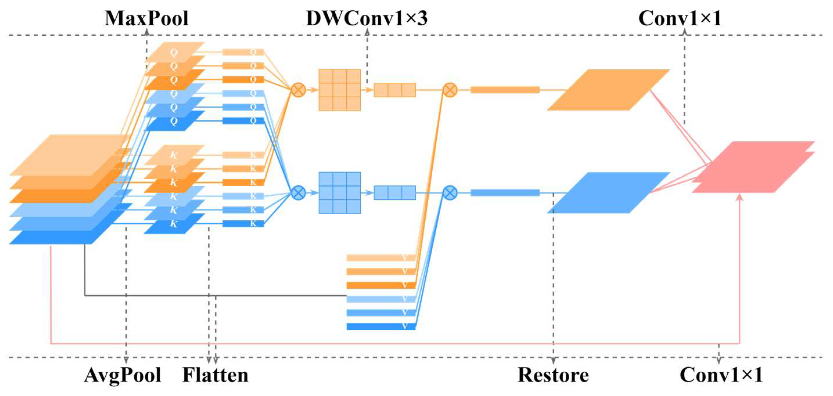
3.3. Spatial Dual-Scale Convolution-Aided Self-Attention Encoder

The spatial-DCSA encoder assembles spatial features hierarchically using a stack of five blocks, and each block contains three layers with a skip connection. As shown in Figure 3a, the first and the third layers are both the 1 × 1 convolutional layers for channel mixing rather than the aim of dimensionality reduction or expansion in the residual [50] or the inverted residual [51] module. A batch normalization (BN) and a rectified linear unit (ReLU) are executed after each layer. The middle layer is a DCSA layer that extracts informative spatial features while maintaining the inherent spectral–spatial data structure. The DCSA layer is shown in Figure 3b. In an attempt to keep the spectral–spatial data structure, the spatial feature extraction can be conducted in groups. Since group convolution is a great substitute for group operation, we directly use it. By aligning the groups in group convolution with the heads in MSA, convolution-aided self-attention can be executed.

First, we use group convolutions with different kernel sizes to transform $X\in {ℝ}^{c\times h\times w}$ into Q, K, and V; the number of groups is g, and the stride is s. As illustrated in Figure 4, when s is 2, the kernel size is also set to 2. When s is 1, the kernel size for obtaining K and V is set to 1 while 3 is for Q, which is termed the dual-scale that helps to fully explore information on different scales without inducing too many parameters. Besides, Q can have a larger receptive field for better guiding the allocations of attention weight.

$$\left\{\begin{array}{cc}Q/K/V={\mathrm{GConv}}_{2\times 2,s=2,groups=g}\left(X\right)\hfill & s=2\hfill \\ Q={\mathrm{GConv}}_{3\times 3,s=1,groups=g}\left(X\right),K/V={\mathrm{GConv}}_{1\times 1,s=1,groups=g}\left(X\right)\hfill & s=1\hfill \end{array}\right.\in {ℝ}^{c\times \frac{h}{s}\times \frac{w}{s}}$$

(9)

where the GConv(·) denotes the group convolution.

Then, a reshape operation is carried out to adjust the data structure for follow-up calculations:

$$Q^{\prime }/K^{\prime }/V^{\prime }=\mathrm{reshape}\left(Q/K/V\right)\in {ℝ}^{g\times \frac{hw}{s^2}\times \frac{c}{g}}$$

(10)

After that, self-attention can be used to calculate spatial attention. Notably, since convolutions naturally have an intuition for positions [43], the positional encoding will not be used in our network

$$\mathrm{DCSA}\left(Q,K,V\right)=\mathrm{softmax}\left(\frac{Q^{\prime }{K^{\prime }}^{\mathrm{T}}}{\sqrt{d_k}}\right)V^{\prime }$$

(11)

where $d_k=\frac{c}{g}$.

Finally, restoring the data shape: ${ℝ}^{g\times \frac{hw}{s^2}\times \frac{c}{g}}\mapsto {ℝ}^{c\times \frac{h}{s}\times \frac{w}{s}}$.

3.4. Spatial Convolution-Aided Cross-Attention Decoder

The spatial-CCA decoder restores the resolutions of feature maps progressively. For designing a decoder, previous studies have demonstrated the benefits of attaching the low-level but high-resolution features obtained earlier by the encoder to the high-level features in the decoder. Apart from the feature concatenation method proposed in UNet, there are also some other context fusion methods. For example, the UNet transformer [52] used cross-attention in an encoder-decoder skip connection manner, achieving good performance in medical image segmentation. Inspired by it, we adopt a skip connection level cross-attention operation to effectively transfer refined information from the encoder to the decoder.

Symmetrical to the encoder, the decoder is constructed from four CCA blocks and a transposed convolutional block. The difference lies in the middle layer: the encoder utilizes the self-attention mechanism while the decoder adopts the cross-attention mechanism. The CCA layer is shown in Figure 3c; one input $X_{\mathrm{de}}\in {ℝ}^{c\times h\times w}$ comes from the existing block, and another input $X_{en}\in {ℝ}^{c\times \left(h\cdot s\right)\times \left(w\cdot s\right)}$ was obtained earlier from the previous encoder block. The transposed convolution is employed to upsample $X_{de}\in {ℝ}^{c\times h\times w}$ into $Q\in {ℝ}^{c\times \left(h\cdot s\right)\times \left(w\cdot s\right)}$ with a stride s. And two group convolutions with kernel size 1 are used to transform $X_{en}\in {ℝ}^{c\times \left(h\cdot s\right)\times \left(w\cdot s\right)}$ into $K/V\in {ℝ}^{c\times \left(h\cdot s\right)\times \left(w\cdot s\right)}$. Since Q contains high-level information while K and V provide details such as edge and texture, an integration could facilitate feature expression. Thus, the cross-attention is carried out to recalibrate the obtained features, which aggregates low-level but high-resolution features with high-level but low-resolution features. This process can be formulated as follows:

$$\begin{array}{cc}Q=\left\{\begin{array}{cc}{\mathrm{DConv}}_{2\times 2,s=2,groups=g}\left(X_{de}\right)\hfill & s=2\hfill \\ {\mathrm{GConv}}_{1\times 1,s=1,groups=g}\left(X_{\mathrm{de}}\right)\hfill & s=1\hfill \end{array}\right.,& K/V={\mathrm{GConv}}_{1\times 1,s=1,groups=g}\left(X_{en}\right)\end{array}$$

(12)

$$Q^{\prime }/K^{\prime }/V^{\prime }=\mathrm{reshape}\left(Q/K/V\right)\in {ℝ}^{g\times \left(hw\cdot s^2\right)\times \frac{c}{g}}$$

(13)

$$\mathrm{CCA}\left(Q,K,V\right)=\mathrm{softmax}\left(\frac{Q^{\prime }{K^{\prime }}^{\mathrm{T}}}{\sqrt{d_k}}\right)V^{\prime }$$

(14)

$$X_{\mathrm{de}}{}^{\prime }=\mathrm{reshape}\left(\mathrm{CCA}\left(Q,K,V\right)\right)\in {ℝ}^{c\times \left(h\cdot s\right)\times \left(w\cdot s\right)}$$

(15)

where $d_k=\frac{c}{g}$ and DConv(·) denotes the transposed convolution.

4. Experiment

In this section, the proposed UCaT is quantitatively evaluated using three publicly available HSI datasets. These datasets and the implementation details of experiments are briefly introduced at first. Then, the important parameters, such as the input patch size, the network width, and the number of groups, are selected experimentally. After that, extensive experiments are conducted for comparison with several state-of-the-art classification algorithms, evaluating the classification performance of the UCaT. Finally, ablation experiments are carried out to further confirm the effectiveness of the main components.

4.1. Data Description

Three publicly available HSI datasets, i.e., Indian Pines (IP), Pavia University (PU), and Salinas Valley (SV), are used to evaluate the effectiveness of the proposed UCaT, the false-color images and the ground-truth maps are shown in Figure 5.

(1)

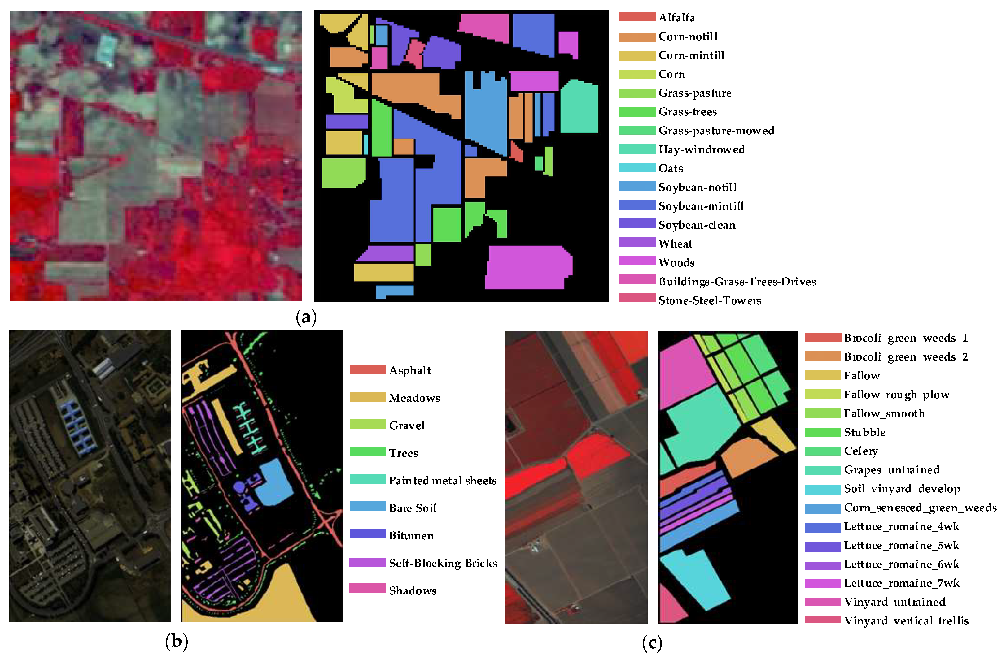
IP dataset: The first dataset was acquired by the Airborne Visible/Infrared Imaging Spectrometer (AVIRIS) sensor over the Indian Pines field in Northwestern Indiana. After discarding some spectral bands that are affected by the water absorption, the remaining 200 bands in a spatial size of 145 × 145 pixels are used for experiments. The dataset has 10,249 labeled pixels that can be partitioned into 16 land cover types.

(2)

PU dataset: The second dataset was gathered by the Reflective Optics System Imaging Spectrometer (ROSIS) sensor at Pavia University, Northern Italy. The image consists of 610 × 340 pixels; among them, 42,776 pixels were labeled. The dataset has 9 types of land cover classes and 103 spectral bands.

(3)

SV dataset: The third dataset was also collected by the AVIRIS sensor over Salinas Valley, California. After removing the water absorption bands, the remaining 204 bands with a spatial size of 512 × 217 pixels are used for experiments. The dataset has 16 land cover classes, and a total of 54,129 pixels were labeled.

4.2. Experimental Setup

(1)

Metrics: Three evaluation metrics, i.e., overall accuracy (OA), average accuracy (AA), and kappa coefficient (K), are used to measure the classification performance quantitatively. To ensure the reliability of the experiment results, all subsequent experiments are repeated ten times, and each is conducted on randomly selected training and testing sets.

(2)

Data partition: For the IP, PU, and SV datasets, 10% (1024 pixels), 5% (2138 pixels), and 3% (1623 pixels), respectively, of the labeled samples, are randomly selected for training. The random seeds for the ten times repeated experiments are set to 0~9 for reducing random error.

(3)

Implementation details: All experiments are implemented with the Python 3.7 compiler and the PyTorch platform, running on a desktop PC with an Intel Core i7-9700 CPU and an NVIDIA GeForce RTX 3080 graphics card. Before training, the original HSI datasets are normalized to the range [0, 1] using the min-max scaling. Then, the cross-entropy loss and the AdamW optimizer (the weight decay is set to 0.03) are used to supervise training. Specifically, we train the network for 105 epochs with a mini-batch size of 128. The learning rate is initialized to 0.03, and then the CosineAnnealingWarmRestarts learning rate scheduler is employed to adjust it, where the number of iterations for the first restart T_0 is set to 5, and the increase factor after each restart T_mult is set to 4.

4.3. Parameter Analysis

The exploration of the main parameters, such as the input patch size, the network width, and the number of groups, is indispensable since they have considerable influences on the classification performance. The proper parameters will be selected through experiments.

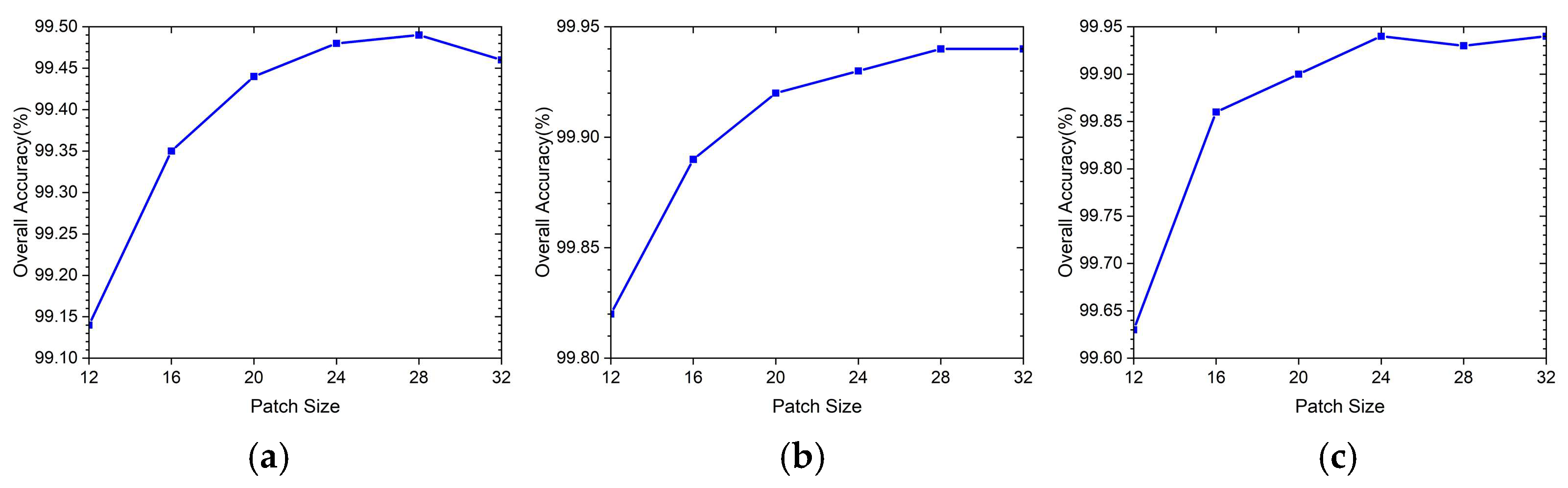
4.3.1. Influence of Patch Size

To a certain extent, the larger input patch size could produce more neighborhood information for classification. However, as the patch size continues to grow, the computational complexity and the number of parameters increase significantly, yet the gain in classification performance decelerates gradually. We therefore compare the classification performance with different input patch sizes in the range of {12 × 12, 16 × 16, 20 × 20, 24 × 24, 28 × 28, 32 × 32} and report the variation trends in Figure 6. It can be found that the OA curves show an improvement along with the expansion of patch size, especially for the IP and SV datasets. However, if the patch size exceeds 20 × 20, the increase in OA is not statistically significant. Accordingly, follow-up experiments set the patch sizes for the IP, PU, and SV datasets to 24 × 24, 20 × 20, and 24 × 24, respectively, as a compromise between classification performance and computational complexity.

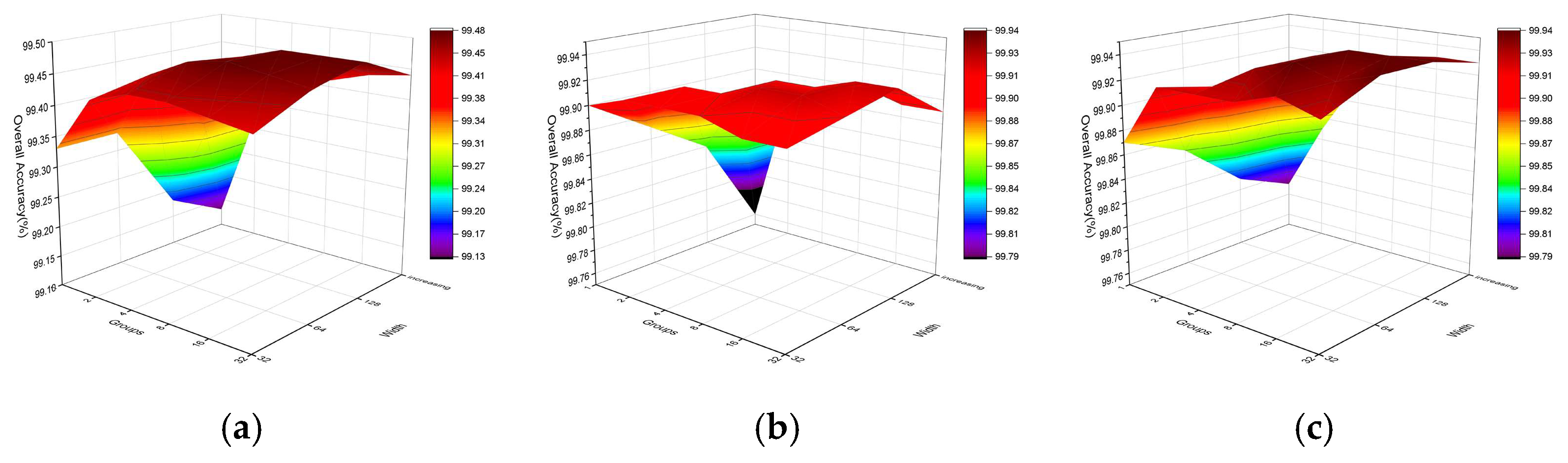
4.3.2. Influence of Network Width and the Number of Groups

We report the classification results under different types of network width: {32, 64, 128, [32, 64, 128, 256, 512]} with different numbers of groups: {1, 2, 4, 8, 16, 32}, the last setting of the network width represents the increasing width of each block. As seen in Figure 7, when the width is 64, the accuracy is generally better. The accuracy presents an increasing and then a slightly downward trend with the increasing numbers of groups. We set the network width to 64 and the number of groups to 8 for follow-up experiments.

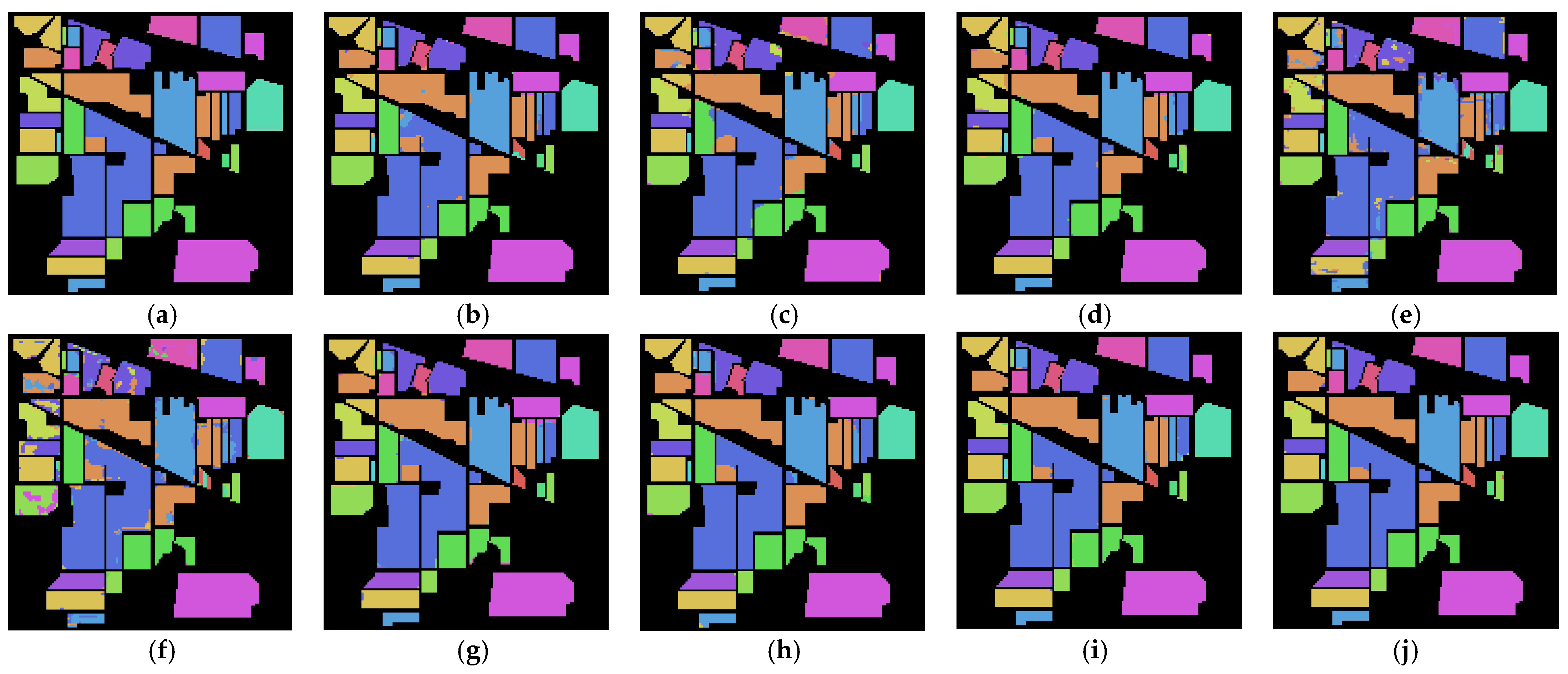
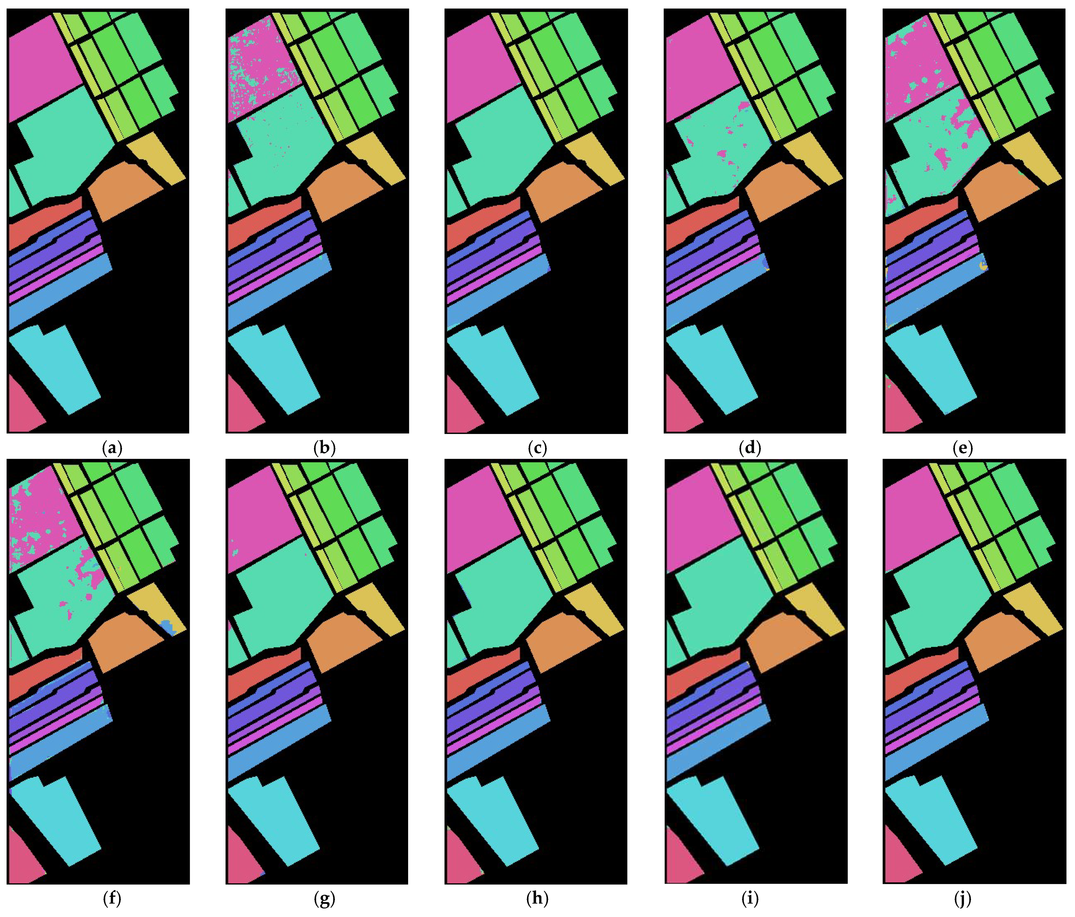
4.4. Classification Results

Eight state-of-the-art networks, including CNN- and transformer-based networks, and segmentation networks, are selected for comparative experiments to analyze the classification performance of the proposed network in HSI classification. They are spectral–spatial residual network (SSRN) [25], hybrid spectral CNN (HybridSN) [28], double-branch dual-attention mechanism network (DBDA) [53], vision transformer (ViT) [31], spectral former (SF) [33], spectral–spatial feature tokenization transformer (SSFTT) [1], UNet [47], and UNet transformer (UT) [52]. The hyperparameters of the SSRN, HybridSN, DBDA, SF, and SSFTT are set based on the recommendations in their respective literature. As for the ViT, UNet, and UT, the hyperparameters are consistent with our proposed UCaT for a fair comparison.

Detailed results of these networks on the IP, PU, and SV datasets are presented in

Table 1. Comparison experimental results on the IP dataset using 10% training samples.

Class	CNN-Based			Transformer-Based			Segmentation Network		Proposed
	SSRN	HybridSN	DBDA	ViT	SF	SSFTT	UNet	UT	UCaT
1	87.81	86.10	91.95	62.68	39.02	94.39	95.85	96.34	98.05
2	97.99	94.20	98.10	89.35	89.25	98.48	98.91	98.86	99.25
3	98.05	96.20	97.87	88.73	88.70	97.95	98.85	98.38	99.22
4	97.23	93.24	96.34	88.26	78.12	96.71	97.28	98.73	99.20
5	96.60	95.59	95.45	91.68	93.56	96.05	96.58	96.94	97.68
6	99.59	98.19	98.90	98.01	97.84	98.33	99.56	99.36	99.88
7	99.20	88.00	98.00	80.40	56.80	99.60	92.40	90.00	96.80
8	99.79	99.70	99.86	98.79	99.56	99.98	99.98	99.91	100
9	80.00	62.22	90.00	81.67	75.00	85.00	93.89	93.33	100
10	96.83	95.46	96.79	87.89	87.21	96.99	98.66	98.37	99.29
11	98.47	98.36	98.26	96.03	90.95	99.05	99.72	99.65	99.86
12	96.52	91.85	96.76	79.59	80.82	96.91	98.15	98.28	99.03
13	99.78	98.76	99.03	99.51	98.00	99.73	99.68	99.41	99.95
14	99.37	98.89	99.51	98.16	96.69	99.80	99.92	99.76	99.99
15	97.90	94.41	97.23	85.53	89.05	98.42	92.48	99.42	99.54
16	99.05	86.91	95.60	99.76	97.14	92.74	96.31	98.69	97.74
OA (%)	98.17	96.42	97.99	92.42	90.79	98.34	98.81	99.02	99.48
AA (%)	96.51	92.38	96.85	89.13	84.86	96.88	97.39	97.84	99.09
K (%)	97.91	95.91	97.70	91.34	89.50	98.10	98.65	98.88	99.41

,

Table 2. Comparison experimental results on the PU dataset using 5% training samples.

Class	CNN-Based			Transformer-Based			Segmentation Network		Proposed
	SSRN	HybridSN	DBDA	ViT	SF	SSFTT	UNet	UT	UCaT
1	99.75	99.82	99.72	94.91	96.19	99.93	99.74	99.79	99.95
2	99.82	99.99	99.94	98.02	99.38	99.96	100	100	100
3	97.17	98.33	98.55	82.69	90.92	98.04	99.76	99.97	99.96
4	98.93	96.96	98.52	97.52	96.19	98.16	99.06	99.08	99.23
5	100	99.70	99.88	99.91	100	99.85	100	100	100
6	99.74	99.87	98.81	76.47	97.60	99.93	100	100	100
7	99.81	99.76	99.87	83.86	87.55	99.95	99.26	100	100
8	98.15	98.35	98.84	92.00	91.83	98.74	99.59	99.76	99.96
9	99.80	97.30	98.82	99.28	97.64	97.03	99.80	99.89	99.61
OA (%)	99.47	99.43	99.48	93.34	97.00	99.56	99.82	99.88	99.92
AA (%)	99.24	98.90	99.22	91.63	95.26	99.07	99.69	99.83	99.86
K (%)	99.29	99.25	99.31	91.10	96.02	99.41	99.76	99.83	99.90

and

Table 3. Comparison experimental results on the SV dataset using 3% training samples.

Class	CNN-Based			Transformer-Based			Segmentation Network		Proposed
	SSRN	HybridSN	DBDA	ViT	SF	SSFTT	UNet	UT	UCaT
1	99.75	99.96	99.79	99.80	99.15	100	99.94	99.95	100
2	97.94	100	100	98.89	99.72	100	99.91	99.96	100
3	99.09	100	99.97	99.54	99.00	100	99.91	100	99.99
4	99.60	99.10	99.16	97.96	99.03	99.94	99.57	99.59	99.93
5	93.58	99.43	98.18	99.24	99.12	99.37	99.55	99.69	99.51
6	100	99.85	99.89	99.74	99.56	99.99	100	100	100
7	99.97	99.92	99.88	98.89	99.23	99.92	99.91	99.96	100
8	95.99	99.58	97.83	91.15	88.15	99.42	99.76	99.98	100
9	99.99	100	99.94	99.66	99.60	100	99.95	99.96	100
10	99.43	99.27	98.92	93.54	94.28	99.80	99.25	99.48	99.83
11	98.49	99.69	99.49	95.55	93.77	99.87	99.62	99.32	99.86
12	99.93	99.85	99.96	99.51	99.02	99.96	100	100	100
13	99.62	99.48	98.67	99.11	98.20	99.78	99.74	99.78	99.91
14	99.01	98.98	97.94	99.02	97.04	99.86	99.31	99.06	99.48
15	89.49	99.64	96.92	83.33	87.01	99.46	99.86	99.85	99.95
16	99.42	99.94	99.39	97.29	97.66	99.65	98.45	99.19	99.99
OA (%)	97.13	99.71	98.83	94.98	94.83	99.73	99.75	99.84	99.94
AA (%)	98.21	99.67	99.12	97.01	96.85	99.81	99.67	99.74	99.90
K (%)	96.80	99.68	98.70	94.40	94.25	99.70	99.72	99.82	99.93

, where the best results are in bold. We can observe that the classification results of CNN-based networks are generally better than those of transformer-based networks except for the SSFTT. This suggests that CNNs can capture more detailed information than pure transformers for refined classification. Since the SSFTT used convolutional layers to extract low-level spectral and spatial features first and then developed the transformer encoder module for capturing global contextual dependencies, it produced better results than pure CNNs or transformers. Moreover, we can also observe that the traditional patch-wise classification networks are generally worse than the segmentation networks, possibly because it is not robust to force the labels of a patch to be the label of its center pixel. Besides, despite the total number of labeled training pixels being the same, the segmentation networks can repeatedly use the training pixels in different patches, which enriches the feature representation. Most notably, among all the networks, the proposed UCaT achieves the highest classification results with 99.48% OA, 99.09% AA, 99.41% K on the IP dataset, 99.92% OA, 99.86% AA, 99.90% K on the PU dataset, and 99.94% OA, 99.90% AA, 99.93% K on the SV dataset. The high classification accuracy confirms that our proposed network can exploit both the advantages of CNNs and transformers. Besides, it can improve the classification performance of the segmentation networks.

Specifically, on the IP dataset (see Table 1), the classification results of the proposed UCaT are significantly higher than those of the other networks. It achieves the highest accuracy in 14 of a total of 16 land cover categories. And the classification results of all the land cover categories are more than 96% despite the extremely unbalanced data distribution of the IP dataset, which demonstrates that our proposed network can still achieve promising results under the extremely unbalanced data distribution.

The improvement in the PU dataset is also obvious (see Table 2). Out of a total of 9 land cover categories, 7 can achieve the highest accuracy. All the land cover classes could achieve a classification accuracy of over 99.2%. In particular, classes 2, 5, 6, and 7, which are meadows, painted metal sheets, bare soil, and bitumen, respectively, achieve a straight 100% accuracy.

On the SV dataset (see Table 3), all the classes could achieve a classification accuracy of over 99.4%. Classes 1, 2, 6, 7, 8, 9, and 12, which are Brocoli_green_weeds_1, Brocoli_green_weeds_2, Stubble, Celery, Grapes_untrained, Soil_vinyard_develop, and Lettuce_romaine_5wk, respectively, could attain an accuracy of 100%.

The classification maps of the comparison networks and the proposed network on the three datasets are shown in Figure 8, Figure 9 and Figure 10. On the whole, it can be seen that the proposed UCaT can obtain better classification maps than others, showing its superiority in HSI classification. Specifically, first, the classification maps of the proposed network are the closest to the ground truth maps for all the three datasets. Moreover, it can be seen that there is no apparent noise scatter in the classification maps of the proposed network for all the three datasets, which demonstrates that the proposed network could effectively eliminate semantic ambiguity by capturing pixel-level spatial dependencies. Moreover, the edges in the classification maps of the proposed network are also relatively smooth, especially on the PU dataset, which may suggest that the proposed UCaT has the spatial feature representation ability.

4.5. Ablation Study

The proposed UCaT contains three key components: the spectral-GSA component, the spatial-DCSA encoder, and the spatial-CCA decoder. This part investigates the necessity of the three components experimentally on the IP dataset using 10% training data. Then, the effectiveness of the particular strategies in the spatial-DCSA encoder and the spatial-CCA decoder is also evaluated.

The classification results in the absence of the three components are evaluated in terms of OA, AA, and K. If the spatial-DCSA or the spatial-CCA is not used, then the 1 × 1 convolution (2 × 2 convolution or 2 × 2 transposed convolution for the encoder or decoder, respectively, when the stride is 2) is utilized as the substitute for it. If the spectral-GSA component is removed, then the 1 × 1 convolution shall be used for dimensionality reduction. As listed in

Table 4. Ablation experiments of the three main components on the IP dataset.

Spectral-GSA	Spatial-DCSA	Spatial-CCA	OA (%)	AA (%)	K (%)
√	√	√	99.48	99.09	99.41
√	√		99.39	98.78	99.31
√		√	99.38	98.94	99.29
√			98.97	97.74	98.82
	√	√	99.42	99.02	99.34

, combining all three components can achieve the best classification performance. The classification results decrease in the absence of the spatial-DCSA or the spatial-CCA, indicating that they do help in spatial feature learning; however, if the spatial-DCSA and the spatial-CCA are both absent, the classification results drop sharply. A possible reason is that the network can capture informative spatial features by either of the two components, and when one is absent, the other will work. However, the network can only achieve the highest classification results when the two components work collaboratively. Moreover, the decline in classification results in the absence of the spectral-GSA component, which, to some extent, confirms that the spectral-GSA can capture more discriminative spectral features. To make the difference easier to observe, an additional experiment was also conducted by reducing the proportion of training data to 5%. The vanilla UCaT achieves the higher classification accuracy with 97.99% OA, 90.92% AA, 97.71% K, and it obtains 97.59% OA, 90.61% AA, 97.25% K in the absence of the spectral-GSA. The decline in OA is 0.4%, further indicating that the spectral-GSA can be helpful in feature learning.

Moreover, to verify the effectiveness of the dual-scale strategy in the spatial-DCSA encoder, we conduct experiments under a series of different kernel sizes for obtaining Q, K, and V when the stride is 1. From

Table 5. Classification results of the UCaT with different kernel sizes for the spatial-DCSA encoder on the IP dataset.

Q	K/V	OA (%)	AA (%)	K (%)	Params
1	1	99.36	98.88	99.27	175k
3	1	99.48	99.09	99.41	187k
3	3	99.46	98.92	99.39	212k

, it can be seen that when the kernel size for obtaining Q, K, and V is 1, the classification results are the worst compared with the other configurations. Changing the kernel size for obtaining Q into 3 can improve the OA, AA, and K by 0.12%, 0.21%, and 0.14%, respectively, and the parameters increase by 12k. However, when the kernel sizes for obtaining K and V are also changed into 3, the classification results do not have further improvement anymore, and the number of parameters continues to increase. In summary, the dual-scale strategy can achieve better classification results without inducing too many parameters, demonstrating its effectiveness.

Furthermore,

Table 6. Classification results of the UCaT with different feature fusion methods for the spatial-CCA decoder on the IP dataset.

	OA (%)	AA (%)	K (%)	Params
Cross-Attention	99.48	99.09	99.41	187k
Concatenate	99.39	98.94	99.30	207k
Add	99.41	98.98	99.33	190k

lists the classification results under the cross-attention, the concatenate, and the add approaches in the spatial-CCA decoder. By contrast, the network outperforms other strategies when using the cross-attention strategy for information fusion between the encoder and decoder, confirming the effectiveness of the cross-attention strategy in the spatial-CCA decoder.

5. Discussion

To make the UCaT more explainable, the heatmaps [54] which indicate the salient regions for classification, are generated with respect to different land cover classes on the IP dataset. The ground truth map of the cropped HSI patch is shown in Figure 11a. We chose two kinds of classes, i.e., the Corn-notill and the Stone-Steel-Towers, for illustration. The heatmaps that take all the pixels in the same class and one of a pixel in this class as outputs for calculating the gradients of loss are shown in Figure 11. When taking all the pixels in the same class as output, we can observe that the heatmaps are similar to the land cover locations of this class, which confirms that the UCaT has the capacity for spatial information perception.

It can also be found that when taking one pixel as output for backpropagation, the heatmaps are almost the same as the heatmaps that take all pixels in the same class as output for backpropagation. This is proof that the proposed UCaT can capture pixel-level spatial dependencies.

In sum, these heatmaps indicate the advantages of the cooperation among convolution, MSA, and the U-shaped segmentation architecture. With regard to a whole patch, the network differentiates several homogeneous regions by spatial relations and gives comprehensive consideration, which helps to eliminate semantic ambiguity caused by the inadequacy of training samples. With respect to a pixel, the network can capture pixel-level spatial dependencies, which finds similar pixels to assist the classification of this pixel. We think it is a good quality for HSI classification.

6. Conclusions

In this paper, a novel U-shaped convolution-aided transformer (UCaT) network with spectral attention and spatial attention is proposed for HSI classification, which tries to take full advantage of CNNs and transformers for better classification. This network grafts group convolutions to MSA as compensation for loss of local information. And different from other combination methods, the UCaT is particularly adaptable to the characteristics of HSI data. It decouples channels into groups when extracting informative features and simultaneously maintaining the inherent spectral–spatial data structure. Moreover, the dual-scale strategy and the cross-attention strategy are adopted for richer feature representation. On the IP, PU, and SV datasets, the proposed method could achieve an overall accuracy of 99.48%, 99.92%, and 99.94%, respectively. The computational complexity is acceptable since the calculation is conducted on the cropped HSI patches instead of the raw dataset. The quite competitive classification performance suggests that the proposed network has the potential to be generally applied to varied HSI analysis tasks and is worth conducting further research. In the future, we will continue to study how to extract more discriminative spectral features and how to improve the generalization ability.

References

1. Sun, L.; Zhao, G.; Zheng, Y.; Wu, Z. Spectral–Spatial Feature Tokenization Transformer for Hyperspectral Image Classification. IEEE Trans. Geosci. Remote Sens. 2022, 60, 5522214. [Google Scholar] [CrossRef]
2. Xu, Y.; Du, B.; Zhang, L. Beyond the Patchwise Classification: Spectral–Spatial Fully Convolutional Networks for Hyperspectral Image Classification. IEEE Trans. Big Data 2020, 6, 492–506. [Google Scholar] [CrossRef]
3. Xue, X.; Zhang, H.; Fang, B.; Bai, Z.; Li, Y. Grafting Transformer on Automatically Designed Convolutional Neural Network for Hyperspectral Image Classification. IEEE Trans. Geosci. Remote Sens. 2022, 60, 5531116. [Google Scholar] [CrossRef]
4. Zhou, Q.; Zhou, S.; Shen, F.; Yin, J.; Xu, D. Hyperspectral Image Classification Based on 3-D Multihead Self-Attention Spectral–Spatial Feature Fusion Network. IEEE J. Sel. Top. Appl. Earth Observ. Remote Sens. 2023, 16, 1072–1084. [Google Scholar] [CrossRef]
5. Zhang, H.; Yao, J.; Ni, L.; Gao, L.; Huang, M. Multimodal Attention-Aware Convolutional Neural Networks for Classification of Hyperspectral and LiDAR Data. IEEE J. Sel. Top. Appl. Earth Observ. Remote Sens. 2023, 16, 3635–3644. [Google Scholar] [CrossRef]
6. Yu, H.; Xu, Z.; Zheng, K.; Hong, D.; Yang, H.; Song, M. MSTNet: A Multilevel Spectral–Spatial Transformer Network for Hyperspectral Image Classification. IEEE Trans. Geosci. Remote Sens. 2022, 60, 5532513. [Google Scholar] [CrossRef]
7. Cai, Y.; Liu, X.; Cai, Z. BS-Nets: An End-to-End Framework for Band Selection of Hyperspectral Image. IEEE Trans. Geosci. Remote Sens. 2020, 58, 1969–1984. [Google Scholar] [CrossRef]
8. Zhang, Z.; Li, T.; Tang, X.; Hu, X.; Peng, Y. CAEVT: Convolutional Autoencoder Meets Lightweight Vision Transformer for Hyperspectral Image Classification. Sensors 2022, 22, 3902. [Google Scholar] [CrossRef]
9. Qiao, X.; Roy, S.K.; Huang, W. Rotation Is All You Need: Cross Dimensional Residual Interaction for Hyperspectral Image Classification. IEEE J. Sel. Top. Appl. Earth Observ. Remote Sens. 2023, 16, 5387–5404. [Google Scholar] [CrossRef]
10. Borsoi, R.A.; Imbiriba, T.; Bermudez, J.C.M.; Richard, C.; Chanussot, J.; Drumetz, L.; Tourneret, J.Y.; Zare, A.; Jutten, C. Spectral Variability in Hyperspectral Data Unmixing: A Comprehensive Review. IEEE Geosci. Remote Sens. Mag. 2021, 9, 223–270. [Google Scholar] [CrossRef]
11. Alkhatib, M.Q.Q.; Al-Saad, M.; Aburaed, N.; Almansoori, S.; Zabalza, J.; Marshall, S.; Al-Ahmad, H. Tri-CNN: A Three Branch Model for Hyperspectral Image Classification. Remote Sens. 2023, 15, 316. [Google Scholar] [CrossRef]
12. Zhou, P.; Han, J.; Cheng, G.; Zhang, B. Learning Compact and Discriminative Stacked Autoencoder for Hyperspectral Image Classification. IEEE Trans. Geosci. Remote Sens. 2019, 57, 4823–4833. [Google Scholar] [CrossRef]
13. Ma, X.; Wang, H.; Geng, J. Spectral–Spatial Classification of Hyperspectral Image Based on Deep Auto-Encoder. IEEE J. Sel. Top. Appl. Earth Observ. Remote Sens. 2016, 9, 4073–4085. [Google Scholar] [CrossRef]
14. Hang, R.; Liu, Q.; Hong, D.; Ghamisi, P. Cascaded Recurrent Neural Networks for Hyperspectral Image Classification. IEEE Trans. Geosci. Remote Sens. 2019, 57, 5384–5394. [Google Scholar] [CrossRef]
15. Mou, L.; Ghamisi, P.; Zhu, X.X. Deep Recurrent Neural Networks for Hyperspectral Image Classification. IEEE Trans. Geosci. Remote Sens. 2017, 55, 3639–3655. [Google Scholar] [CrossRef]
16. Wu, H.; Prasad, S. Semi-Supervised Deep Learning Using Pseudo Labels for Hyperspectral Image Classification. IEEE Trans. Image Process. 2018, 27, 1259–1270. [Google Scholar] [CrossRef] [PubMed]
17. Li, S.; Song, W.; Fang, L.; Chen, Y.; Ghamisi, P.; Benediktsson, J.A. Deep Learning for Hyperspectral Image Classification: An Overview. IEEE Trans. Geosci. Remote Sens. 2019, 57, 6690–6709. [Google Scholar] [CrossRef]
18. Haut, J.M.; Paoletti, M.E.; Plaza, J.; Li, J.; Plaza, A. Active Learning with Convolutional Neural Networks for Hyperspectral Image Classification Using a New Bayesian Approach. IEEE Trans. Geosci. Remote Sens. 2018, 56, 6440–6461. [Google Scholar] [CrossRef]
19. Chen, Y.; Jiang, H.; Li, C.; Jia, X.; Ghamisi, P. Deep Feature Extraction and Classification of Hyperspectral Images Based on Convolutional Neural Networks. IEEE Trans. Geosci. Remote Sens. 2016, 54, 6232–6251. [Google Scholar] [CrossRef]
20. Song, W.; Li, S.; Fang, L.; Lu, T. Hyperspectral Image Classification with Deep Feature Fusion Network. IEEE Trans. Geosci. Remote Sens. 2018, 56, 3173–3184. [Google Scholar] [CrossRef]
21. Lu, Z.; Xu, B.; Sun, L.; Zhan, T.; Tang, S. 3-D Channel and Spatial Attention Based Multiscale Spatial–Spectral Residual Network for Hyperspectral Image Classification. IEEE J. Sel. Top. Appl. Earth Observ. Remote Sens. 2020, 13, 4311–4324. [Google Scholar] [CrossRef]
22. Xue, Z.; Xu, Q.; Zhang, M. Local Transformer with Spatial Partition Restore for Hyperspectral Image Classification. IEEE J. Sel. Top. Appl. Earth Observ. Remote Sens. 2022, 15, 4307–4325. [Google Scholar] [CrossRef]
23. Shu, Z.; Liu, Z.; Zhou, J.; Tang, S.; Yu, Z.; Wu, X.J. Spatial–Spectral Split Attention Residual Network for Hyperspectral Image Classification. IEEE J. Sel. Top. Appl. Earth Observ. Remote Sens. 2023, 16, 419–430. [Google Scholar] [CrossRef]
24. Li, X.; Ding, M.; Pižurica, A. Deep Feature Fusion via Two-Stream Convolutional Neural Network for Hyperspectral Image Classification. IEEE Trans. Geosci. Remote Sens. 2020, 58, 2615–2629. [Google Scholar] [CrossRef]
25. Zhong, Z.; Li, J.; Luo, Z.; Chapman, M. Spectral–Spatial Residual Network for Hyperspectral Image Classification: A 3-D Deep Learning Framework. IEEE Trans. Geosci. Remote Sens. 2018, 56, 847–858. [Google Scholar] [CrossRef]
26. Zhao, H.; Wang, C.; Chen, H.; Chen, T.; Deng, W. A Hybrid Classification Method with Dual-Channel CNN and KELM for Hyperspectral Remote Sensing Images. Int. J. Remote Sens. 2023, 44, 289–310. [Google Scholar] [CrossRef]
27. Zhang, H.; Li, Y.; Zhang, Y.; Shen, Q. Spectral–Spatial Classification of Hyperspectral Imagery Using a Dual-Channel Convolutional Neural Network. Remote Sens. Lett. 2017, 8, 438–447. [Google Scholar] [CrossRef]
28. Roy, S.K.; Krishna, G.; Dubey, S.R.; Chaudhuri, B.B. HybridSN: Exploring 3-D–2-D CNN Feature Hierarchy for Hyperspectral Image Classification. IEEE Geosci. Remote Sens. Lett. 2020, 17, 277–281. [Google Scholar] [CrossRef]
29. Huang, W.; Zhao, Z.; Sun, L.; Ju, M. Dual-Branch Attention-Assisted CNN for Hyperspectral Image Classification. Remote Sens. 2022, 14, 6158. [Google Scholar] [CrossRef]
30. Vaswani, A.; Shazeer, N.; Parmar, N.; Uszkoreit, J.; Jones, L.; Gomez, A.N.; Kaiser, L.; Polosukhin, I. Attention Is All You Need. arXiv 2017, arXiv:1706.03762. [Google Scholar] [CrossRef]
31. Dosovitskiy, A.; Beyer, L.; Kolesnikov, A.; Weissenborn, D.; Zhai, X.; Unterthiner, T.; Dehghani, M.; Minderer, M.; Heigold, G.; Gelly, S.; et al. An Image Is Worth 16x16 Words: Transformers for Image Recognition at Scale. arXiv 2020, arXiv:2010.11929. [Google Scholar] [CrossRef]
32. He, X.; Chen, Y.; Lin, Z. Spatial–Spectral Transformer for Hyperspectral Image Classification. Remote Sens. 2021, 13, 498. [Google Scholar] [CrossRef]
33. Hong, D.; Han, Z.; Yao, J.; Gao, L.; Zhang, B.; Plaza, A.; Chanussot, J. SpectralFormer: Rethinking Hyperspectral Image Classification with Transformers. IEEE Trans. Geosci. Remote Sens. 2022, 60, 5518615. [Google Scholar] [CrossRef]
34. He, J.; Zhao, L.; Yang, H.; Zhang, M.; Li, W. HSI-BERT: Hyperspectral Image Classification Using the Bidirectional Encoder Representation from Transformers. IEEE Trans. Geosci. Remote Sens. 2020, 58, 165–178. [Google Scholar] [CrossRef]
35. Liang, M.; He, Q.; Yu, X.; Wang, H.; Meng, Z.; Jiao, L. A Dual Multi-Head Contextual Attention Network for Hyperspectral Image Classification. Remote Sens. 2022, 14, 3091. [Google Scholar] [CrossRef]
36. Wang, S.; Liu, Z.; Chen, Y.; Hou, C.; Liu, A.; Zhang, Z. Expansion Spectral-Spatial Attention Network for Hyperspectral Image Classification. IEEE J. Sel. Top. Appl. Earth Observ. Remote Sens. 2023, 16, 6411–6427. [Google Scholar] [CrossRef]
37. Peng, Y.; Liu, Y.; Tu, B.; Zhang, Y. Convolutional Transformer-Based Few-Shot Learning for Cross-Domain Hyperspectral Image Classification. IEEE J. Sel. Top. Appl. Earth Observ. Remote Sens. 2023, 16, 1335–1349. [Google Scholar] [CrossRef]
38. Yuan, K.; Guo, S.; Liu, Z.; Zhou, A.; Yu, F.; Wu, W. Incorporating Convolution Designs into Visual Transformers. In Proceedings of the 2021 IEEE/CVF International Conference on Computer Vision (ICCV), Montreal, QC, Canada, 10–17 October 2021; pp. 559–568. [Google Scholar]
39. Touvron, H.; Cord, M.; Douze, M.; Massa, F.; Sablayrolles, A.; Jegou, H. Training Data-Efficient Image Transformers & Distillation Through Attention. In Proceedings of the International Conference on Machine Learning (ICML), Electr Network, Online, 18–24 July 2021; pp. 7358–7367. [Google Scholar]
40. Bai, J.; Wen, Z.; Xiao, Z.; Ye, F.; Zhu, Y.; Alazab, M.; Jiao, L. Hyperspectral Image Classification Based on Multibranch Attention Transformer Networks. IEEE Trans. Geosci. Remote Sens. 2022, 60, 5535317. [Google Scholar] [CrossRef]
41. Sun, H.; Zheng, X.; Lu, X.; Wu, S. Spectral–Spatial Attention Network for Hyperspectral Image Classification. IEEE Trans. Geosci. Remote Sens. 2020, 58, 3232–3245. [Google Scholar] [CrossRef]
42. Liu, Z.; Lin, Y.; Cao, Y.; Hu, H.; Wei, Y.; Zhang, Z.; Lin, S.; Guo, B. Swin Transformer: Hierarchical Vision Transformer Using Shifted Windows. In Proceedings of the 2021 IEEE/CVF International Conference on Computer Vision (ICCV), Montreal, QC, Canada, 10–17 October 2021; pp. 9992–10002. [Google Scholar]
43. Wu, H.; Xiao, B.; Codella, N.; Liu, M.; Dai, X.; Yuan, L.; Zhang, L. CvT: Introducing Convolutions to Vision Transformers. In Proceedings of the 2021 IEEE/CVF International Conference on Computer Vision (ICCV), Montreal, QC, Canada, 10–17 October 2021; pp. 22–31. [Google Scholar]
44. Graham, B.; El-Nouby, A.; Touvron, H.; Stock, P.; Joulin, A.; Jégou, H.; Douze, M. LeViT: A Vision Transformer in ConvNet’s Clothing for Faster Inference. In Proceedings of the 2021 IEEE/CVF International Conference on Computer Vision (ICCV), Montreal, QC, Canada, 10–17 October 2021; pp. 12239–12249. [Google Scholar]
45. Liu, H.; Li, W.; Xia, X.G.; Zhang, M.; Gao, C.Z.; Tao, R. Central Attention Network for Hyperspectral Imagery Classification. EEE Trans. Neural Netw. Learn. Syst. 2022, 34, 8989–9003. [Google Scholar] [CrossRef]
46. Yang, K.; Sun, H.; Zou, C.; Lu, X. Cross-Attention Spectral–Spatial Network for Hyperspectral Image Classification. IEEE Trans. Geosci. Remote Sens. 2022, 60, 5518714. [Google Scholar] [CrossRef]
47. Ronneberger, O.; Fischer, P.; Brox, T. U-Net: Convolutional Networks for Biomedical Image Segmentation. In Proceedings of the 18th International Conference on Medical Image Computing and Computer-Assisted Intervention (MICCAI), Munich, Germany, 5–9 October 2015; pp. 234–241. [Google Scholar]
48. Audebert, N.; Saux, B.L.; Lefevre, S. Deep Learning for Classification of Hyperspectral Data: A Comparative Review. IEEE Geosci. Remote Sens. Mag. 2019, 7, 159–173. [Google Scholar] [CrossRef]
49. Fu, J.; Liu, J.; Tian, H.; Li, Y.; Bao, Y.; Fang, Z.; Lu, H. Dual Attention Network for Scene Segmentation. In Proceedings of the 2019 IEEE/CVF Conference on Computer Vision and Pattern Recognition (CVPR), Long Beach, CA, USA, 15–20 June 2019; pp. 3141–3149. [Google Scholar]
50. He, K.; Zhang, X.; Ren, S.; Sun, J. Deep Residual Learning for Image Recognition. In Proceedings of the 2016 IEEE Conference on Computer Vision and Pattern Recognition (CVPR), Las Vegas, NV, USA, 27–30 June 2016; pp. 770–778. [Google Scholar]
51. Sandler, M.; Howard, A.; Zhu, M.; Zhmoginov, A.; Chen, L.C. MobileNetV2: Inverted Residuals and Linear Bottlenecks. In Proceedings of the 2018 IEEE/CVF Conference on Computer Vision and Pattern Recognition, Salt Lake City, UT, USA, 18–23 June 2018; pp. 4510–4520. [Google Scholar]
52. Petit, O.; Thome, N.; Rambour, C.; Themyr, L.; Collins, T.; Soler, L. U-Net Transformer: Self and Cross Attention for Medical Image Segmentation. In Proceedings of the 12th International Workshop on Machine Learning in Medical Imaging (MLMI 2021), Strasbourg, France, 27 September 2021; pp. 267–276. [Google Scholar]
53. Li, R.; Zheng, S.; Duan, C.; Yang, Y.; Wang, X. Classification of Hyperspectral Image Based on Double-Branch Dual-Attention Mechanism Network. Remote Sens. 2020, 12, 582. [Google Scholar] [CrossRef]
54. Selvaraju, R.R.; Cogswell, M.; Das, A.; Vedantam, R.; Parikh, D.; Batra, D.; IEEE. Grad-CAM: Visual Explanations from Deep Networks via Gradient-based Localization. In Proceedings of the 16th IEEE International Conference on Computer Vision (ICCV), Venice, Italy, 22–29 October 2017; pp. 618–626. [Google Scholar]
Figure 1. Network structure of the proposed UCaT.
Remotesensing 16 00288 g001
Figure 2. Calculation flowchart of the spectral-GSA component.
Remotesensing 16 00288 g002
Figure 3. Illustration of the DCSA and CCA blocks. (a) The DCSA block or the CCA block; (b) the middle layer of the DCSA block; (c) the middle layer of the CCA block.
Remotesensing 16 00288 g003
Figure 4. Implementation details of the convolutional projection. (a) Stride is 2; (b) Stride is 1.
Remotesensing 16 00288 g004
Figure 5. Dataset visualization. (a) IP dataset; (b) PU dataset; (c) SV dataset.
Remotesensing 16 00288 g005
Figure 6. OAs (%) of UCaT with different sizes of input patches. (a) On the IP dataset, (b) on the PU dataset, and (c) on the SV dataset.
Remotesensing 16 00288 g006
Figure 7. OAs (%) of the UCaT with different network widths and numbers of groups. (a) On the IP dataset, (b) on the PU dataset, and (c) on the SV dataset.
Remotesensing 16 00288 g007
Figure 8. Illustration of the classification maps on the IP dataset. (a) Ground truth; (b) SSRN; (c) HybridSN; (d) DBDA; (e) ViT; (f) SF; (g) SSFTT; (h) UNet; (i) UT; (j) proposed network. Colors have the same meaning as in Figure 5.
Remotesensing 16 00288 g008
Figure 9. Illustration of the classification maps on the PU dataset. (a) Ground truth; (b) SSRN; (c) HybridSN; (d) DBDA; (e) ViT; (f) SF; (g) SSFTT; (h) UNet; (i) UT; (j) proposed network. Colors have the same meaning as in Figure 5.
Remotesensing 16 00288 g009aRemotesensing 16 00288 g009b
Figure 10. Illustration of the classification maps on the SV dataset. (a) Ground truth; (b) SSRN; (c) HybridSN; (d) DBDA; (e) ViT; (f) SF; (g) SSFTT; (h) UNet; (i) UT; (j) proposed network. Colors have the same meaning as in Figure 5.
Remotesensing 16 00288 g010
Figure 11. Class-specific visualizations. (a) Ground truth; (b) ground truth of Corn-notill; (cg) heatmaps of blocks 1, 3, 5, 7, 9; (h) a random pixel of Corn-notill; (im) heatmaps of block 1, 3, 5, 7, 9; (n) ground truth of Stone-Steel-Towers; (os) heatmaps of block 1, 3, 5, 7, 9; (t) a random pixel of Stone-Steel-Towers; (uy) heatmaps of block1, 3, 5, 7, 9. Colors have the same meaning as in Figure 5 and Figure 7.
Remotesensing 16 00288 g011