Multipath-Closure Calibration of Stereo Camera and 3D LiDAR Combined with Multiple Constraints

Abstract

Stereo cameras can capture the rich image textures of a scene, while LiDAR can obtain accurate 3D coordinates of point clouds of a scene. They complement each other and can achieve comprehensive and accurate environment perception through data fusion. The primary step in data fusion is to establish the relative positional relationship between the stereo cameras and the 3D LiDAR, known as extrinsic calibration. Existing methods establish the camera–LiDAR relationship by constraints of the correspondence between different planes in the images and point clouds. However, these methods depend on the planes and ignore the multipath-closure constraint among the camera–LiDAR–camera sensors, resulting in poor robustness and accuracy of the extrinsic calibration. This paper proposes a trihedron as the calibration object to effectively establish various coplanar and collinear constraints between stereo cameras and 3D LiDAR. With the various constraints, the multipath-closure constraint between the three sensors is further formulated for the extrinsic calibration. Firstly, the coplanar and collinear constraints between the camera–LiDAR–camera are built using the trihedron calibration object. Then, robust and accurate coplanar constraint information is extracted through iterative maximum a posteriori (MAP) estimation. Finally, a multipath-closure extrinsic calibration method for multi-sensor systems is developed with structurally mutual validation between the cameras and the LiDAR. Extensive experiments are conducted on simulation data with different noise levels and a large amount of real data to validate the accuracy and robustness of the proposed calibration algorithm.

1. Introduction

The combination of stereo cameras and 3D LiDAR is widely used in robotics [1,2,3,4,5,6,7,8], mobile measurement [9,10], and autonomous driving [11,12]. The stereo camera can provide color, texture information, and dense depth data of the scene, but the resulting depth data is not highly accurate and is easily affected by the environment. LiDAR can provide accurate depth information and is not easily affected by the environment, but the resulting depth data is sparse and lacks texture and color information. Therefore, the different information provided by the two systems complement one another, and more accurate environmental perception can be achieved through fusion of the two data sources. However, since the installation positions of the stereo camera and the 3D LiDAR are different, the primary problem in the fusion of the two data sources is the extrinsic calibration between the sensors, which involves calculating the rotation matrix and the translation vector between the different coordinate systems of the sensors.

The extrinsic calibration between the stereo camera and the 3D LiDAR relies on the geometric correspondence of specific calibration objects between the three sensors. The chessboard calibration object [13,14,15,16,17,18] is the most widely used in this context. Unnikrishnan et al. [19], Pandey et al. [20], Mirazei et al. [21], Liu et al. [22], Khoscovian et al. [23], Zhou et al. [24], Lu et al. [25], Liu et al. [26], and Li et al. [27] established coplanar constraint relationships through checkerboard calibration objects to accomplish the extrinsic calibration of cameras and 3D LiDAR. Zhou et al. [28] added edge detection of the checkerboard on the basis of Unnikrishnan’s method, establishing coplanar and collinear constraint relationships. However, due to the limitation of the distance between LiDAR points, the edge of the checkerboard plane could not be accurately obtained. Thus, Zhou’s method cannot establish an accurate collinear constraint relationship, which primarily uses the geometric constraint relationship of coplanarity. Although the extrinsic calibration between sensors can be completed through a single coplanar constraint relationship, to obtain more accurate extrinsic parameters more accurate geometric constraint relationships need to be explored.

Closed-loop interconnection is formed between three sensors, including the stereo cameras and the 3D LiDAR. The three extrinsic parameters between the three sensors are interrelated, and the direct extrinsic parameters between two sensors can be derived from their round-way interconnection with the third sensor. However, due to the noise of the data collected by the sensor, there is inevitable error in the extrinsic parameter, which will accumulate with the round-way iterative calibration between neighboring sensors. Based on the closed-loop interconnection between sensors, the closed-loop interconnection constraint between the three relative extrinsic parameters can be constructed, reducing the accumulated error and improving the calibration accuracy [29,30,31,32]. Numerous studies have been conducted in the calibration of multi-sensor systems. Quoc et al. [33] proposed a method of calibrating the extrinsic parameters of multi-sensor systems through sensor grouping, where each sensor group produces 3D data in a unified form and the extrinsic parameters between groups are calibrated through the geometric constraints established by the calibration object. Li et al. [34] and Li et al. [35] regarded the stereo camera and the LiDAR as a sensor group, respectively, and applied Quoc’s method to the extrinsic calibration of the stereo camera and the 2D LiDAR. These methods did not consider the closed-loop interconnection constraints between multiple sensors, which would introduce cumulative errors and affect the accuracy of the calibration algorithm. Joris et al. [36], LIU et al. [37], and Sim [38] considered the closed-loop interconnection of multiple sensors and added closed-loop interconnection constraints to calibrate multi-sensor systems. However, it is impossible to directly obtain the analytical solution of the extrinsic calibration in solving the extrinsic parameters of the sensors. Instead, an optimization function based on the data collected by the sensors needs to be established, and the numerical solution of the extrinsic parameters are obtained by iterative optimization using nonlinear optimization methods. The closed-loop interconnection constraints proposed by Joris et al. [36], LIU et al. [37], and Sim [38] are in the matrix form independent of the sensor’s data, making it difficult to optimize them iteratively in the nonlinear optimization process.

Aimed at the problem that the current method primarily uses the single coplanar constraint and does not make full use of the closed-loop interconnection between sensors, this paper proposes a multipath-closure calibration method of the stereo cameras and the 3D LiDAR with multiple constraints, and the main innovations are as follows:

Firstly, although coplanar constraint relationships are widely used and mature, obtaining more accurate extrinsic parameter results requires exploring more accurate geometric constraint relationships. Therefore, this paper uses trihedrons as the calibration object [39] to establish various geometric constraint relationships, such as coplanar and collinear, and iteratively estimates the noise parameters of the point cloud to obtain more robust and accurate geometric constraint relationships.

Secondly, a camera–LiDAR–camera closed-loop interconnection exists in both stereo camera systems and 3D LiDAR systems, and many methods disregard this closed-loop interconnection, which can introduce accumulated errors during calibration and affect calibration accuracy. Even if there are methods that consider the application of closed-loop interconnection constraints to reduce the cumulative error, the closed-loop interconnection constraints of these methods are challenging to iterate in the process of nonlinear optimization. Therefore, this paper proposes a new type of closed-loop constraint called the multipath-closure constraint. The constraint converts the closed-loop interconnection constraint in the form of a matrix independent of the data collected by the sensor into the vector form of data correlation, which can efficiently perform iterative optimization in the nonlinear solution while reducing the accumulated error.

Finally, this paper conducted extensive experiments on real and simulated data. In the actual experiment, the algorithm proposed in this paper was quantitatively evaluated for its applicability in real scenes by projecting LiDAR points onto images. In the simulation experiment, both the accuracy and the robustness of the algorithm under different noise and pose conditions were quantitatively evaluated, along with the influence of different constraint relationships on the extrinsic parameter results. The experimental results demonstrate the accuracy and robustness of the algorithm proposed in this paper.

2. Methodology

2.1. Problem Definition

For the multi-sensor system used in this paper, composed of stereo cameras and a 3D LiDAR, as shown in Figure 1, a world coordinate system (${\mathit{O}}_{\mathit{w}}-{\mathit{X}}_{\mathit{w}}{\mathit{Y}}_{\mathit{w}}{\mathit{Z}}_{\mathit{w}}$) is established, with one vertex of a trihedron calibration object as the origin. Two camera coordinate systems, (${\mathit{O}}_{{\mathit{C}}_{\mathit{1}}}-{\mathit{X}}_{{\mathit{C}}_{\mathit{1}}}{\mathit{Y}}_{{\mathit{C}}_{\mathit{1}}}{\mathit{Z}}_{{\mathit{C}}_{\mathit{1}}}$) and (${\mathit{O}}_{{\mathit{C}}_{\mathit{2}}}-{\mathit{X}}_{{\mathit{C}}_{\mathit{2}}}{\mathit{Y}}_{{\mathit{C}}_{\mathit{2}}}{\mathit{Z}}_{{\mathit{C}}_{\mathit{2}}}$), are established, with the optical centers of the two cameras as the origins, respectively, and the imaging plane parallel to the XOY plane and the Z axis pointing forward. With the LiDAR scanning center as the origin and the horizontal scanning surface as the XOY surface, the LiDAR coordinate system (${\mathit{O}}_{\mathit{L}}-{\mathit{X}}_{\mathit{L}}{\mathit{Y}}_{\mathit{L}}{\mathit{Z}}_{\mathit{L}}$) is established according to the right-hand rule, where the coordinates of the LiDAR point, ${\mathit{P}}^L$, in the two camera coordinate systems can be expressed as ${\mathit{P}}^{C_1}=\left(x_{C_1},y_{C_1},z_{C_1}\right)$ and ${\mathit{P}}^{C_2}=\left(x_{C_2},y_{C_2},z_{C_2}\right)$, and the homogeneous coordinates on the image plane are ${\mathit{q}}^{C_1}=\left(u_{C_1},v_{C_1},1\right)$ and ${\mathit{q}}^{C_2}=\left(u_{C_2},v_{C_2},1\right)$. According to the position relationship $\left[{\mathit{R}}_L^{C_1},{\mathit{T}}_L^{C_1}\right]$ between the No.1 camera coordinate system and the LiDAR coordinate system, the relationship between the LiDAR point, ${\mathit{P}}^L$, and the corresponding point, ${\mathit{P}}^{C_1}$, in the No.1 camera coordinate system can be obtained by

$${\mathit{P}}^{C_1}={\mathit{R}}_L^{C_1}{\mathit{P}}^L+{\mathit{T}}_L^{C_1}$$

(1)

In Equation (1), ${\mathit{R}}_L^{C_1}$ is the rotation matrix and ${\mathit{T}}_L^{C_1}$ is the translation vector. Similarly, based on the positional relationship between the coordinate systems of the No.2 camera and the LiDAR $\left[{\mathit{R}}_L^{C_2},{\mathit{T}}_L^{C_2}\right]$ and the positional relationship between the coordinate systems of the No.1 camera and the No.2 camera $\left[{\mathit{R}}_{C_1}^{C_2},{\mathit{T}}_{C_1}^{C_2}\right]$, we can obtain the relationship between the LiDAR point, ${\mathit{P}}^L$, and the corresponding point ${\mathit{P}}^{C_2}$, in the coordinate system of the No.2 camera, as well as the relationship between ${\mathit{P}}^{C_2}$ and ${\mathit{P}}^{C_1}$:

$$\begin{array}{cc}\hfill {\mathit{P}}^{C_2}& ={\mathit{R}}_L^{C_2}{\mathit{P}}^L+{\mathit{T}}_L^{C_2}\hfill \end{array}$$

(2a)

$$\begin{array}{cc}\hfill {\mathit{P}}^{C_2}& ={\mathit{R}}_{C_1}^{C_2}{\mathit{P}}^{C_1}+{\mathit{T}}_{C_1}^{C_2}\hfill \end{array}$$

(2b)

According to the pinhole imaging model, the relationship between the points ${\mathit{P}}^{C_1}$ and ${\mathit{P}}^{C_2}$ in the camera coordinates system and the corresponding image points ${\mathit{q}}^{C_1}$ and ${\mathit{q}}^{C_2}$ can be derived by

$$\begin{array}{cc}\hfill {\mathit{q}}^{C_1}& =s{\mathit{K}}^{C_1}{\mathit{P}}^{C_1}\hfill \end{array}$$

(3a)

$$\begin{array}{cc}\hfill {\mathit{q}}^{C_2}& =s{\mathit{K}}^{C_2}{\mathit{P}}^{C_2}\hfill \end{array}$$

(3b)

In Equation (3), ${\mathit{K}}^{C_1}$ and ${\mathit{K}}^{C_2}$ represent the intrinsic indexes of two cameras, which can be obtained in advance through camera calibration, while s denotes the scale factor.

2.2. The Multipath-Closure Calibration Method with Multiple Constraints

The extrinsic calibration of the stereo camera and the 3D LiDAR involves two aspects: one is the pair-wise calibration of multiple sensors and the other is the optimization of closed-loop interconnection between multiple sensors. The calibration of multiple sensors depends on the multiple geometric constraint relationships established by the calibration object, and the more geometric constraint relationships established by the calibration object, the higher the accuracy of the extrinsic calibration. The planar characteristics of the checkerboard calibration object provide accurate coplanar constraint relations, which are widely used in the extrinsic calibration of sensors. However, the low scanning resolution of LiDAR and the significant distance between points make it difficult to accurately scan the edges of a checkerboard, and it is impossible to establish accurate line constraint relationships directly. A trihedron calibration object can provide three robust plane parameters in image data and LiDAR point clouds, establish three coplanar constraint relationships, and obtain three precise plane intersection lines through the three robust planes. The three intersection lines correspond one-to-one in image and point clouds, establishing three accurate line constraint relationships. Therefore, this paper chooses a trihedron as the calibration object to establish accurate coplanar and collinear geometric constraint relationships. Furthermore, more accurate coplanar and collinear constraint relationships are obtained by modeling the noise of the point cloud. In addition, based on the camera–LiDAR–camera multipath-closure structure of the stereo camera and 3D LiDAR, we establish multipath-closure constraint relationships to reduce accumulated errors in the calibration process and improve calibration accuracy.

This section mainly introduces how to establish various geometric constraint relationships through the trihedron calibration object and how to achieve accurate extrinsic calibration parameters through the multipath-closure constraint between three sensors. As shown in Figure 1, the trihedron calibration object is composed of three checkerboard grids placed perpendicular to one another, which can provide the parameters of three checkerboard grid planes and the intersection line parameters of the planes, building geometric constraint relationships such as coplanarity and collinearity. Meanwhile, the three sensors form a multipath-closure interconnection, which can establish the multipath-closure constraint.

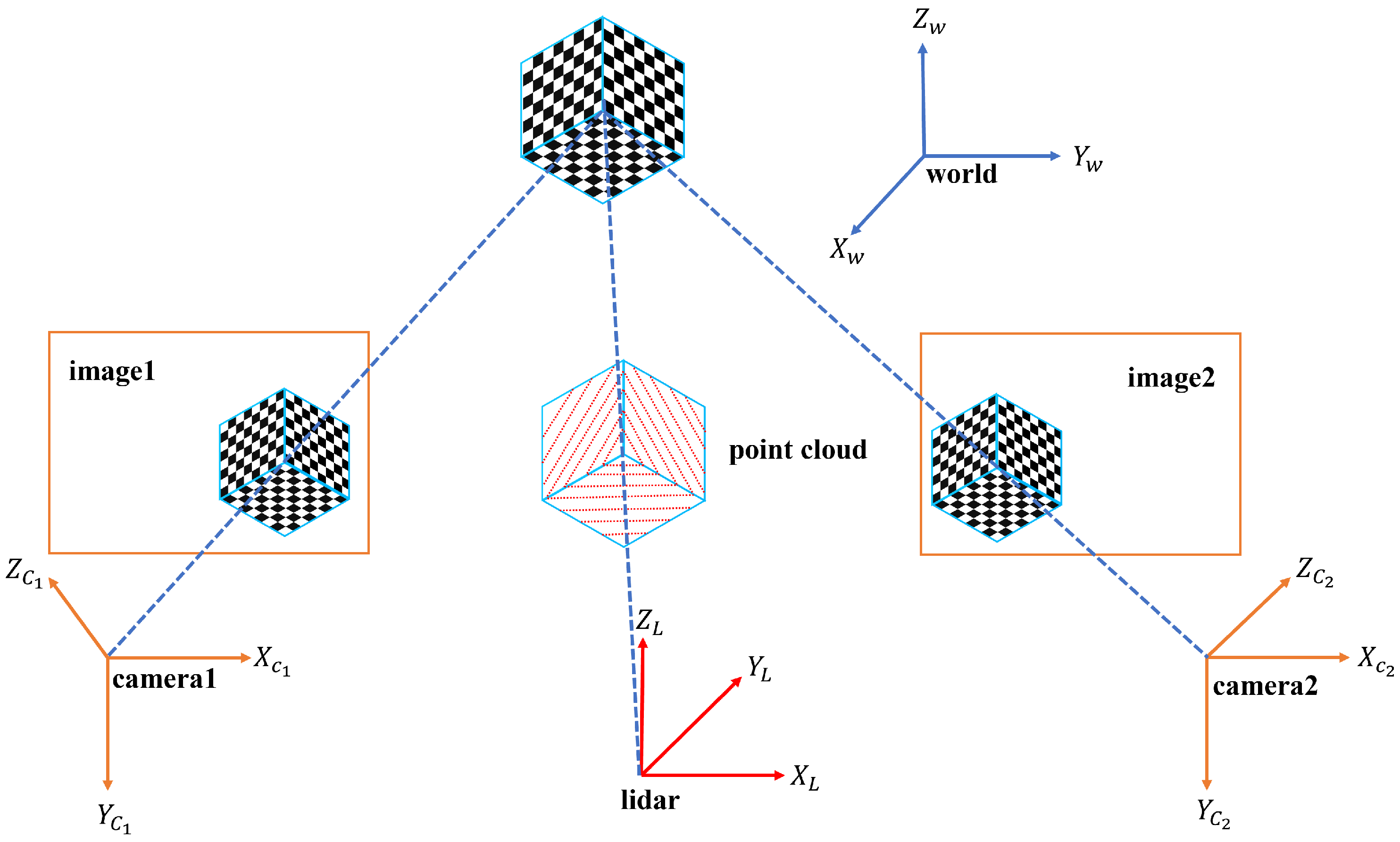
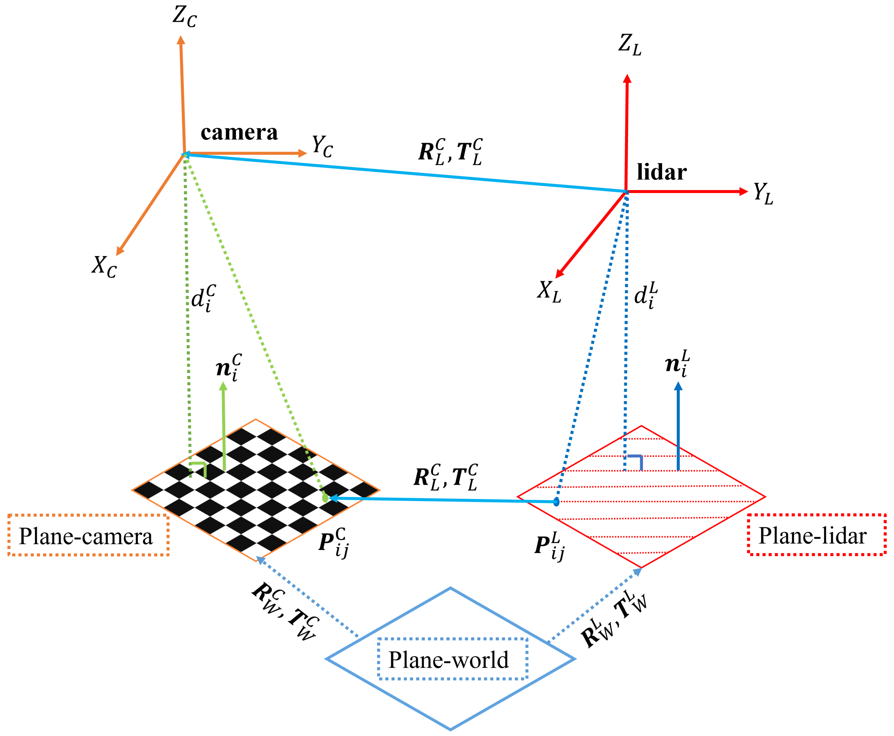
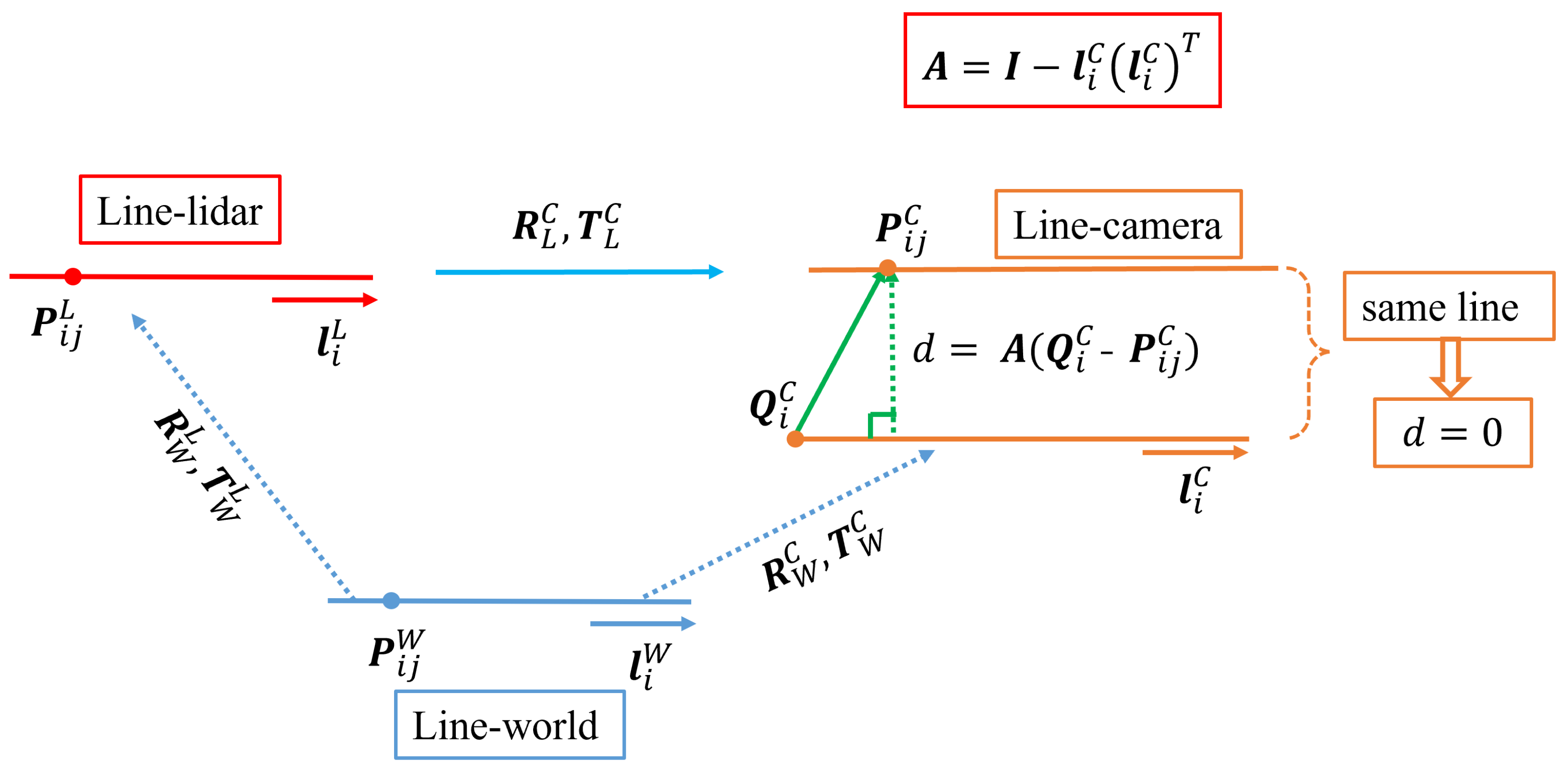
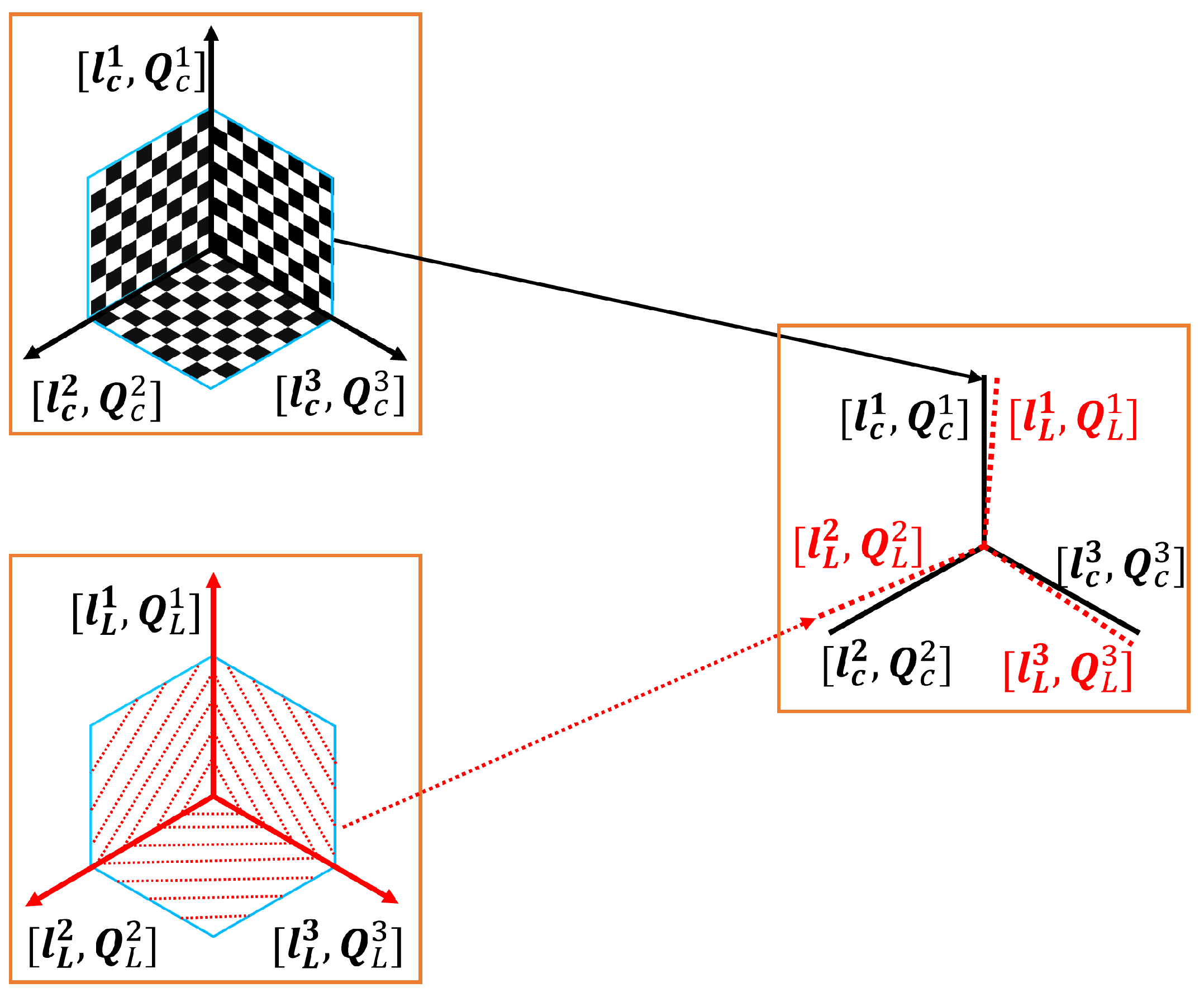
2.2.1. Geometric Constraint Relationships Established by Trihedron Calibration Object

The extrinsic calibration of sensors depends on geometric constraints established by the calibration object. The establishment of geometric constraints originates from the geometric information, such as lines and planes, obtained from the sensor’s calibration data. As shown in Figure 2, three checkerboard planes, ${\mathit{\pi }}_1^L,{\mathit{\pi }}_2^L,{\mathit{\pi }}_3^L$, of the trihedron calibration object, as well as three plane intersection lines, ${\mathit{l}}_1^L,{\mathit{l}}_2^L,{\mathit{l}}_3^L$, can be obtained from the point cloud data acquired by the LiDAR. Similarly, three checkerboard planes, ${\mathit{\pi }}_1^C,{\mathit{\pi }}_2^C,{\mathit{\pi }}_3^C$, three plane intersection lines, ${\mathit{l}}_1^I,{\mathit{l}}_2^I,{\mathit{l}}_3^I$, and corresponding 3D lines, ${\mathit{l}}_1^C,{\mathit{l}}_2^C,{\mathit{l}}_3^C$, in the camera coordinate system can be obtained from the image data acquired by the camera.

(1) Coplanar constraint: The geometric constraint of coplanarity, collinearity, can be established through the geometric information provided by the calibration object. The coplanar relationship established by the calibration object is shown in Figure 3, and the position relationship between the camera coordinate system and the LiDAR coordinate system is $\left.{\left[\mathit{R}\right.}_L^C,{\mathit{T}}_L^C\right]$. From the planar perspective, the parameters of the same checkerboard plane in the camera coordinate system and the LiDAR coordinate system are $\left[{\mathit{n}}_i^C,d_i^C\right],\left[{\mathit{n}}_i^L,d_i^L\right]$, respectively $(\mathit{i}=1,2,3)$, where ${\mathit{n}}_i^C$ and ${\mathit{n}}_i^L$ represent the normal vectors of the checkerboard plane and ${\mathit{d}}_{\mathit{i}}^{\mathit{C}}$ and ${\mathit{d}}_{\mathit{i}}^{\mathit{L}}$ represent the distance from the coordinate system origin to the checkerboard plane. Vectors have translation invariance, and the relationship between the normal vectors ${\mathit{n}}_i^C$ and ${\mathit{n}}_i^L$ are only related to the rotation matrix ${\mathit{R}}_L^C$:

$${\mathit{R}}_L^C{\mathit{n}}_i^L={\mathit{n}}_i^C$$

(4)

The distance is a scalar quantity with rotational invariance, exactly opposite to the normal vector. The relationship between the distances ${\mathit{d}}_{\mathit{i}}^{\mathit{C}}$ and ${\mathit{d}}_{\mathit{i}}^{\mathit{L}}$ only depends on the translation vector ${\mathit{T}}_L^C$. According to the geometric relationship between the distances ${\mathit{d}}_{\mathit{i}}^{\mathit{C}}$ and ${\mathit{d}}_{\mathit{i}}^{\mathit{L}}$ and the translation vector ${\mathit{T}}_L^C$ in Figure 3, the projection value of the translation vector ${\mathit{T}}_L^C$ on the normal vector ${\mathit{n}}_i^C$ is the difference between the distances:

$${\left({\mathit{n}}_i^C\right)}^T{\mathit{T}}_L^C=d_i^L-d_i^C$$

(5)

Equations (4) and (5) are the coplanar constraint relations obtained from the plane perspective for solving the initial values of the extrinsic parameter $\left.{\left[\mathit{R}\right.}_L^C,{\mathit{T}}_L^C\right]$. Considering from the point perspective, the checkerboard plane $\left[{\mathit{n}}_i^C,d_i^C\right]$ in the camera coordinate system and the checkerboard plane $\left[{\mathit{n}}_i^L,d_i^L\right]$ in the LiDAR coordinate system are the same in space, as shown in Figure 3; the point ${\mathit{P}}_{ij}^L$ on the checkerboard plane $\left[{\mathit{n}}_i^L,d_i^L\right]$ is projected to the point ${\mathit{R}}_L^C{\mathit{P}}_{ij}^L+{\mathit{T}}_L^C$ in the camera coordinate system and is located in the checkerboard plane $\left[{\mathit{n}}_i^C,d_i^C\right]$, and the relationship is as follows:

$${\left({\mathit{n}}_i^C\right)}^T\left({\mathit{R}}_L^C{\mathit{P}}_{ij}^L+{\mathit{T}}_L^C\right)-d_i^C=0$$

(6)

Since the data collected by the sensors are noisy and the data volume is large, Equation (6) cannot be used directly. Thus, the error adjustment function is constructed by Equation (6) and then iteratively solved. Assuming there are data from N poses, according to Equation (6) the error adjustment term corresponding to the point ${\mathit{P}}_{ijk}^L$ on the checkerboard plane j in the pose ${\mathit{i}}^{\mathit{th}}$ can be obtained as

$$e_{plane}\left|{\mathit{P}}_{ijk}^L\right.={\left({\left({\mathit{n}}_{ij}^C\right)}^T\left({\mathit{R}}_L^C{\mathit{P}}_{ijk}^L+{\mathit{T}}_L^C\right)-d_{ij}^C\right)}^2$$

(7)

Accumulating the error adjustment terms for all points to obtain the error adjustment terms for the coplanar constraint is as follows:

$$e_{plane}=\sum _{i=1}^N\sum _{j=1}^3\frac{1}{K_{ij}}\sum _{k=1}^{K_{ij}}{e}_{plane}\left|{\mathit{P}}_{ijk}^L\right.$$

(8)

In Equation (8), $K_{ij}$ represents the number of laser points on the j-th checkerboard plane under the i-th pose.

(2) Collinear constraint: The collinear constraint relationship is shown in Figure 4, and the position relationship between the camera coordinate system and the LiDAR coordinate system is $\left.{\left[\mathit{R}\right.}_L^C,{\mathit{T}}_L^C\right]$, similar to the way of thinking about the coplanar constraint, from the perspective of a straight line: the parameters of the same checkerboard plane intersection line in the camera coordinate system and the LiDAR coordinate system are $\left[{\mathit{l}}_i^C,{\mathit{Q}}_i^C\right],\left[{\mathit{l}}_i^L,{\mathit{Q}}_i^L\right],(\mathit{i}=1,2,3)$, respectively, where ${\mathit{l}}_i^C$ and ${\mathit{l}}_i^L$ are the directional vectors of the intersection lines and ${\mathit{Q}}_i^C$ and ${\mathit{Q}}_i^L$ are the endpoints of the intersection lines. Similar to the normal vectors of the plane, the relationship between the direction vectors ${\mathit{l}}_i^C$ and ${\mathit{l}}_i^L$ only relies on the rotation matrix ${\mathit{R}}_L^C$:

$${\mathit{R}}_L^C{\mathit{l}}_i^L={\mathit{l}}_i^C$$

(9)

The position relationship between the intersection endpoints ${\mathit{Q}}_i^C$ and ${\mathit{Q}}_i^L$ is the position relationship between the two coordinate systems:

$${\mathit{Q}}_i^C={\mathit{R}}_L^C{\mathit{Q}}_i^L+{\mathit{T}}_L^C$$

(10)

Equations (9) and (10) provide a collinearity constraint obtained from a linear perspective, which is used to compute the initial value of the extrinsic parameter $\left.{\left[\mathit{R}\right.}_L^C,{\mathit{T}}_L^C\right]$. Considering from the point perspective, as shown in Figure 4, there exists a straight line $\left[{\mathit{l}}_i^C,{\mathit{Q}}_i^C\right]$ and a point ${\mathit{P}}_{ij}^C$ outside the straight line. The vector $\left({\mathit{P}}_{ij}^C-{\mathit{Q}}_i^C\right)$ connects point ${\mathit{P}}_{ij}^C$ and the endpoint ${\mathit{Q}}_i^C$ of the line projects onto the line direction vector ${\mathit{l}}_i^C$ as a projection vector ${\mathit{l}}_{\Vert }={\left({\mathit{l}}_i^C\right)}^T\left({\mathit{P}}_{ij}^C-{\mathit{Q}}_i^C\right){\mathit{l}}_i^C$, and the projection vector on the perpendicular direction of the line $\left[{\mathit{l}}_i^C,{\mathit{Q}}_i^C\right]$ is

$$\begin{array}{cc}\hfill {\mathit{l}}_{\perp }& =\left({\mathit{P}}_{ij}^C-{\mathit{Q}}_i^C\right)-{\mathit{l}}_{\Vert }\hfill \\ \hfill & =\left({\mathit{P}}_{ij}^C-{\mathit{Q}}_i^C\right)-{\left({\mathit{l}}_i^C\right)}^T\left({\mathit{P}}_{ij}^C-{\mathit{Q}}_i^C\right){\mathit{l}}_i^C\hfill \\ \hfill & =\left({\mathit{P}}_{ij}^C-{\mathit{Q}}_i^C\right)-{\mathit{l}}_i^C{\left({\mathit{l}}_i^C\right)}^T\left({\mathit{P}}_{ij}^C-{\mathit{Q}}_i^C\right)\hfill \\ \hfill & =\left(\mathit{I}-{\mathit{l}}_i^C{\left({\mathit{l}}_i^C\right)}^T\right)\left({\mathit{P}}_{ij}^C-{\mathit{Q}}_i^C\right)\hfill \end{array}$$

(11)

In Equation (11), $\mathit{I}$ represents the unit matrix. As shown in Figure 4, the line $\left[{\mathit{l}}_i^C,{\mathit{Q}}_i^C\right]$ in the camera coordinate system and the line $\left[{\mathit{l}}_i^L,{\mathit{Q}}_i^L\right]$ in the LiDAR coordinate system are the same line in space, then the LiDAR point ${\mathit{P}}_{ij}^L$ on the line $\left[{\mathit{l}}_i^L,{\mathit{Q}}_i^L\right]$ is projected to the point ${\mathit{R}}_L^C{\mathit{P}}_{ij}^L+{\mathit{T}}_L^C$ in the camera coordinate system, which is located on the line $\left[{\mathit{l}}_i^C,{\mathit{Q}}_i^C\right]$; thus, the projection vector of the vector connected by the point ${\mathit{R}}_L^C{\mathit{P}}_{ij}^L+{\mathit{T}}_L^C$ and the endpoint ${\mathit{Q}}_i^C$ in the perpendicular direction of the line $\left[{\mathit{l}}_i^C,{\mathit{Q}}_i^C\right]$ is a zero vector. Substituting the point ${\mathit{R}}_L^C{\mathit{P}}_{ij}^L+{\mathit{T}}_L^C$ and the zero vector ${\mathbf{0}}_{3\times 1}$ into Equation (11) for ${\mathit{P}}_{ij}^L$ and ${\mathit{l}}_{\perp }$, respectively, we can obtain

$$\left(\mathit{I}-{\mathit{l}}_i^C{\left({\mathit{l}}_i^C\right)}^T\right)\left({\mathit{R}}_L^C{\mathit{P}}_{ij}^L+{\mathit{T}}_L^C-{\mathit{Q}}_i^C\right)=0_{3\times 1}$$

(12)

Similar to the coplanar constraint, the error adjustment function is constructed through Equation (12) and then solved iteratively. Assuming that there are N poses of data, according to Equation (12) the error adjustment term corresponding to the point ${\mathit{P}}_{ijk}^L$ on the checkerboard intersection $\mathit{j}$ in the ${\mathit{i}}^{\mathit{th}}$ pose can be written as

$$e_{line}\left|{\mathit{P}}_{ijk}^L\right.={\left|\left(\mathit{I}-{\mathit{l}}_{ij}^C{\left({\mathit{l}}_{ij}^C\right)}^T\right)\left({\mathit{R}}_L^C{\mathit{P}}_{ijk}^L+{\mathit{T}}_L^C-{\mathit{Q}}_{ij}^C\right)\right|}^2$$

(13)

Accumulating the error adjustment terms for all points to obtain the error adjustment terms for the coplanar constraint is as follows:

$$e_{line}=\sum _{i=1}^N\sum _{j=1}^3\frac{1}{K_{ij}}\sum _{k=1}^{K_{ij}}{e}_{line}\left|{\mathit{P}}_{ijk}^L\right.$$

(14)

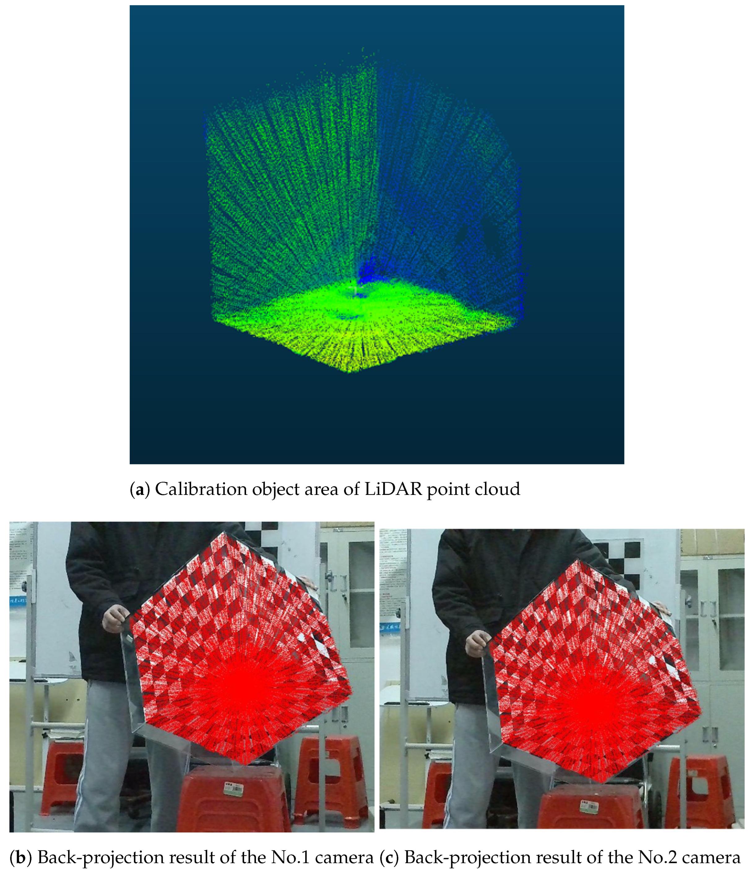
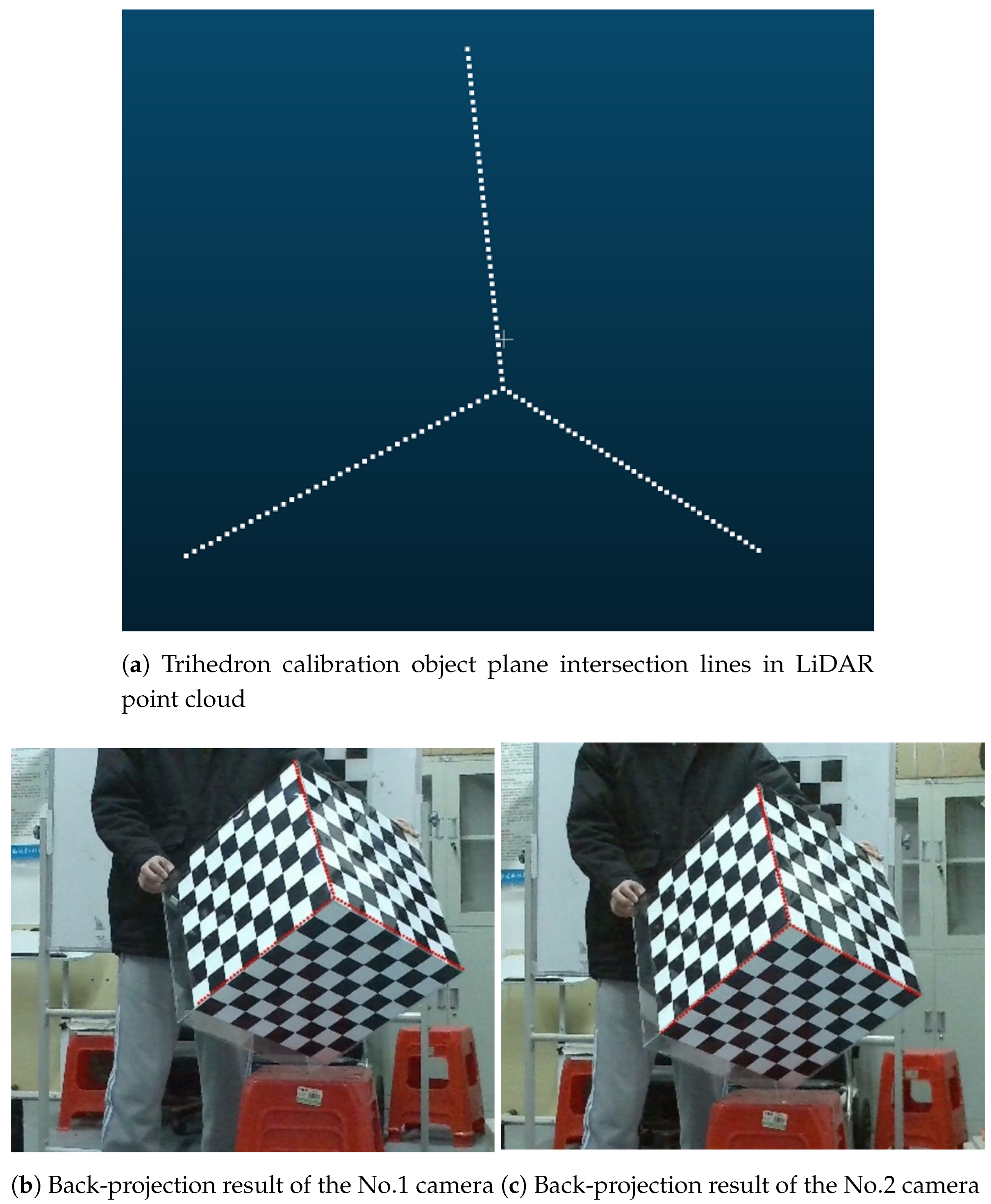
2.2.2. Geometric Information Extraction of Trihedron Calibration Object

Due to the existence of noise in point cloud data, the accurate estimation of geometric feature parameters, such as plane parameters in point clouds, will be affected, which in turn affects the accuracy of coplanar constraints and collinear constraints, and ultimately affects the precision of the calibration. Therefore, this paper estimates the noise parameters through the iterative maximum a posteriori (MAP) of the planar constraint to obtain more accurate checkerboard plane parameters, as well as coplanar and collinear constraints. Specifically, for any LiDAR point ${\mathit{P}}_{ij}=(x,y,z)$, we can obtain its corresponding polar form $(r,\phi ,\theta )$, and the conversion relationship between the two is

$$\begin{array}{cc}\hfill \mathit{x}& =rsin\left(\phi \right)cos\left(\theta \right)\hfill \end{array}$$

(15a)

$$\begin{array}{cc}\hfill \mathit{y}& =rsin\left(\phi \right)sin\left(\theta \right)\hfill \end{array}$$

(15b)

$$\begin{array}{cc}\hfill \mathit{z}& =rcos\left(\phi \right)\hfill \end{array}$$

(15c)

Owing to the change of the surface material, the noise of the LiDAR point ${\mathit{P}}_{ij}$ mainly comes from its distance parameter $\mathit{r}$, in polar coordinates, while the other two angular parameters $\phi ,\theta$ are relatively accurate. Let the coordinates of the truth-value estimation point corresponding to the LiDAR point ${\mathit{P}}_{ij}$ on the checkerboard plane $\left[{\mathit{n}}_i,d_i\right]$ be expressed as ${\mathit{P}}_{ij}^{\prime }=\left(r^{\prime },\phi ,\theta \right)$; the calculation formula for its distance parameter ${\mathit{r}}^{\prime }$ can be obtained as follows:

$$\begin{array}{c}\hfill {\mathit{n}}_i\left[\begin{array}{c}{r}^{\prime }sin\left(\phi \right)cos\left(\theta \right)\\ r^{\prime }sin\left(\phi \right)sin\left(\theta \right)\\ r^{\prime }cos\left(\phi \right)\end{array}\right]-d_i=0\end{array}$$

(16a)

$$\begin{array}{c}\hfill r^{\prime }=\frac{d_i}{n_i^{1}sin\left(\phi \right)cos\left(\theta \right)+n_i^{2}sin\left(\phi \right)sin\left(\theta \right)+n_i^{3}cos\left(\phi \right)}\end{array}$$

(16b)

In Equation (16), ${\mathit{n}}_i=\left[n_i^1,n_i^2,n_i^3\right]$. The above noise estimation idea needs to obtain the exact parameters of the checkerboard plane in the point cloud, but due to the existence of point cloud noise, the exact plane parameters cannot be obtained directly. Therefore, this paper adopts an iterative maximum a posteriori (MAP) estimation method. Firstly, a rough plane parameter is estimated through the RANSAC [40] method. Subsequently, the noise parameters of the point cloud are estimated based on the obtained plane parameters. Then, optimizing the plane parameter by the obtained noise parameter and continuously iterating to obtain the final plane parameter and noise parameter, the specific process is as follows:

I: Obtain the initial parameters using the random sampling consistency (RANSAC) algorithm to obtain the initial plane parameters $\left[{\mathit{n}}_i,d_i\right]$ of the LiDAR point cloud.

II: Calculate the noise parameters. Based on the plane parameters and Equations (15) and (16), obtaining the truth estimation points corresponding to each point in the point cloud, and the noise parameters $\left[\mu ,{\sigma }^2\right]$ are calculated as follows:

$$\begin{array}{cc}\hfill \mu & =\frac{1}{N}\sum _{{\mathit{P}}_{ij}}\left(r-r^{{}^{\prime }}\right)\hfill \end{array}$$

(17a)

$$\begin{array}{cc}\hfill {\sigma }^2& =\frac{1}{N-1}\sum _{{\mathit{P}}_{ij}}{\left(r-r^{{}^{\prime }}-\mu \right)}^2\hfill \end{array}$$

(17b)

In Equation (17), $\mathit{N}$ is the total number of the point cloud.

III: Construct the optimization function of maximum a posteriori (MAP) probability. The planar projection error $e_{{\mathit{P}}_{ij}}={\mathit{n}}_i^T{\mathit{P}}_{ij}-d_i$ for each LiDAR point ${\mathit{P}}_{ij}$; according to the noise parameters of the point cloud, the mean ${\mu }_{{\mathit{P}}_{ij}}$ and the variance ${\sigma }_{{\mathit{P}}_{ij}}^2$ of the $e_{{\mathit{P}}_{ij}}$ can be obtained, and the optimization function of maximum a posteriori (MAP) probability can be written as

$$\left({\mathit{n}}_i, d_i\right)=\underset{{\mathit{n}}_i, {\mathit{d}}_i}{argmin}\sum _i\sum _{{\mathit{P}}_{ij}}\frac{{\left(e_{{\mathit{P}}_{ij}}-{\mu }_{{\mathit{P}}_{ij}}\right)}^2}{{\sigma }_{{\mathit{P}}_{ij}}^2}$$

(18)

IV: Using iterative optimization, we can obtain the optimal estimates of the planar parameters corresponding to Equation (18).

V: Repeat steps II–IV until the results converge, which means that the difference between the error function values corresponding to the optimized and pre-optimized planar parameters is less than a particular threshold value.

With the noise parameters of the point cloud and the more accurate checkerboard plane parameters, the coplanar constraint error adjustment term based on the point cloud noise can be obtained. The surface projection error term of each LiDAR point ${\mathit{P}}_{ij}$ in the camera coordinate system can be expressed as

$$e_{plane}^{{\mathit{P}}_{ij}^L}={\left({\mathit{n}}_i^C\right)}^T\left({\mathit{R}}_L^C{\mathit{P}}_{ij}^L+{\mathit{T}}_L^C\right)-d_i^C$$

(19)

According to the noise parameters $\left[\mu ,{\sigma }^2\right]$ of the point cloud, the mean value ${\mu }_{{\mathit{P}}_{ij}^L}$ and standard deviation ${\sigma }_{{\mathit{P}}_{ij}^L}$ of the $e_{plane}^{{\mathit{P}}_{ij}^L}$ in Equation (19) can be derived as

$$\begin{array}{cc}\hfill {\mu }_{{\mathit{P}}_{ij}^L}& ={\left({\mathit{n}}_i^L\right)}^T\left[\begin{array}{c}sin\left({\phi }_{ij}\right)cos\left({\theta }_{ij}\right)\\ sin\left({\phi }_{ij}\right)sin\left({\theta }_{ij}\right)\\ cos\left({\phi }_{ij}\right)\end{array}\right]\mu \hfill \end{array}$$

(20a)

$$\begin{array}{cc}\hfill {\sigma }_{{\mathit{P}}_{ij}^L}^2& ={\left({\mathit{n}}_i^L\right)}^T\left[\begin{array}{c}sin\left({\phi }_{ij}\right)cos\left({\theta }_{ij}\right)\\ sin\left({\phi }_{ij}\right)sin\left({\theta }_{ij}\right)\\ cos\left({\phi }_{ij}\right)\end{array}\right]{\sigma }^2\hfill \end{array}$$

(20b)

According to Equation (20), given the coordinates of the LiDAR point ${\mathit{P}}_{ij}^L$, the posterior probability distribution of the extrinsic parameters from the LiDAR to the camera can be determined as

$$P\left({\mathit{R}}_L^C,{\mathit{T}}_L^C|{\mathit{P}}_{ij}^L\right)=\frac{exp\left(-\frac{{\left(e_{plane}^{{\mathit{P}}_{ij}^L}-d_i^C-{\mu }_{{\mathit{P}}_{ij}^L}\right)}^2}{2{\sigma }_{{\mathit{P}}_{ij}^L}^2}\right)}{{\sigma }_{{\mathit{P}}_{ij}^L}\sqrt{2\pi }}$$

(21)

This can be estimated from the maximum posterior probability:

$$\begin{array}{cc}\hfill & MLP\left[P\left({\mathit{R}}_L^C,{\mathit{T}}_L^C|{\mathit{P}}_{ij}^L\right)\right]=\underset{{\mathit{R}}_L^C,{\mathit{T}}_L^C}{argmin}-lnP\left({\mathit{R}}_L^C,{\mathit{T}}_L^C|{\mathit{P}}_{ij}^L\right)\hfill \\ \hfill & =\underset{{\mathit{R}}_L^C,{\mathit{T}}_L^C}{argmin}\frac{{\left({\left({\mathit{n}}_i^C\right)}^T\left({\mathit{R}}_L^C{\mathit{P}}_{ij}^L+{\mathit{T}}_L^C\right)-d_i^C-{\mu }_{{\mathit{P}}_{ij}^L}\right)}^2}{{\sigma }_{{\mathit{P}}_{ij}^L}^2}\hfill \end{array}$$

(22)

According to Equation (22), the final error adjustment term for the coplanar constraint based on the noise parameter can be written as

$$e_{plane\_new}=\sum _{i=1}^N\sum _{j=1}^3\frac{1}{K_{ij}}\sum _{k=1}^{K_{ij}}-lnP\left({\mathit{R}}_L^C,{\mathit{T}}_L^C|{\mathit{P}}_{ijk}^L\right)$$

(23)

In Equation (23), the error adjustment term incorporates point cloud noise parameters, rendering it more robust and accurate compared to Equation (8).

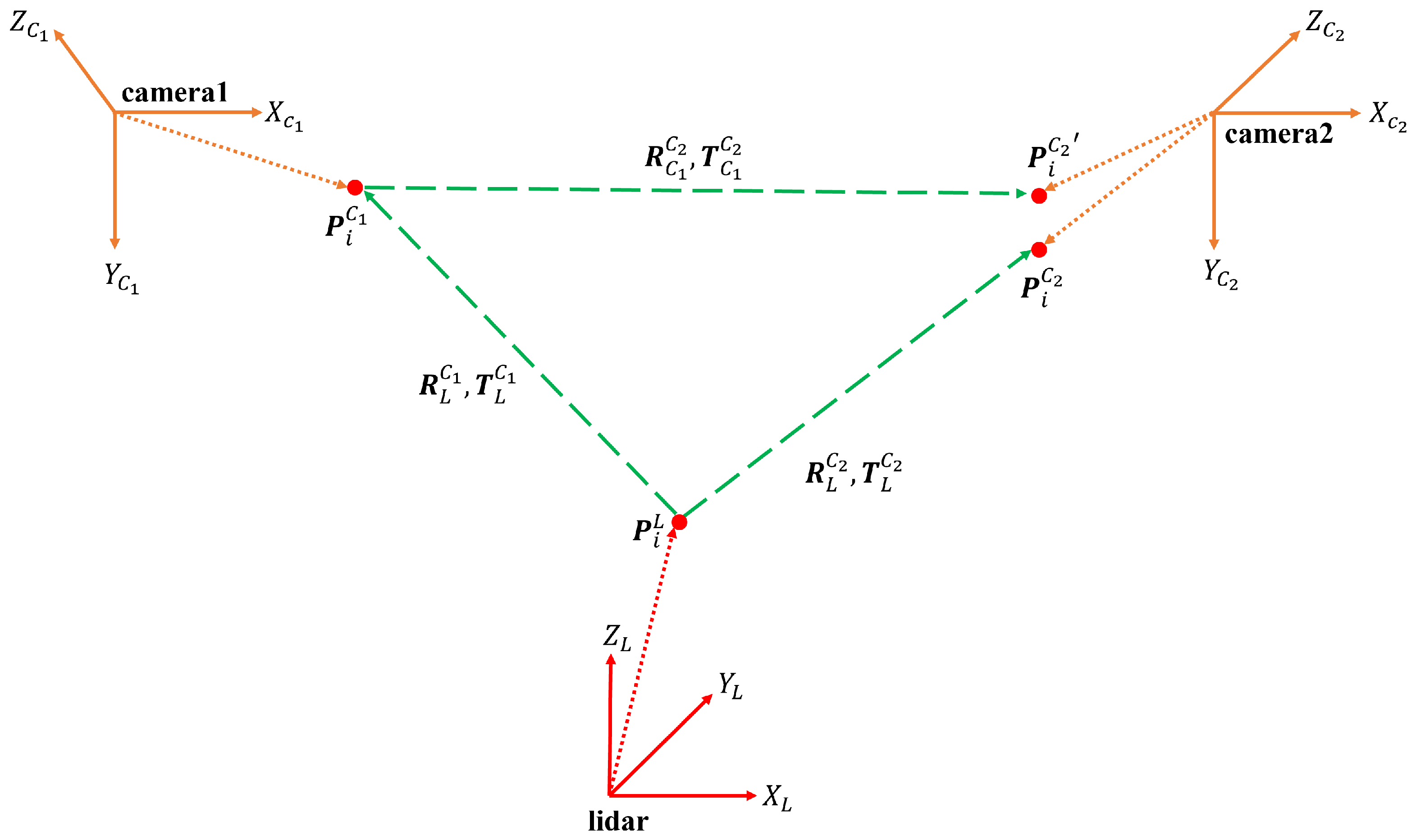
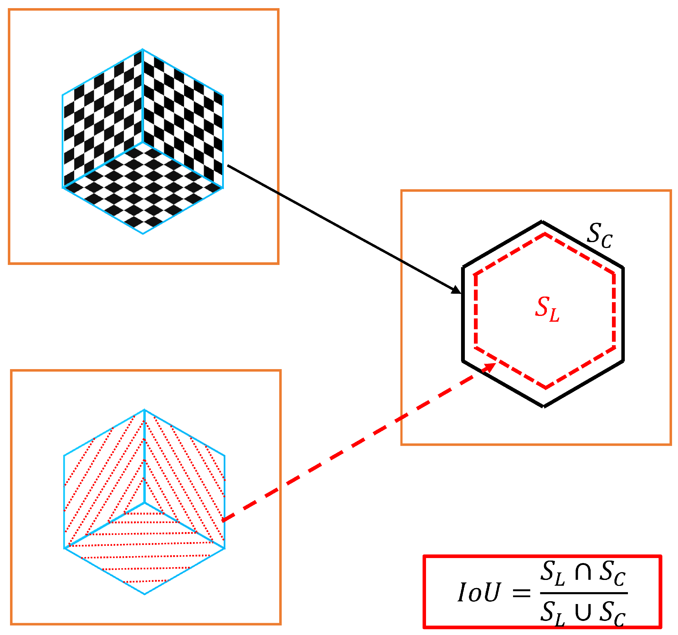
2.2.3. Multipath-Closure Constraint between Sensors

It is illustrated in Figure 5 that the extrinsic parameter $\left[{\mathit{R}}_{C_1}^{C_2},{\mathit{T}}_{C_1}^{C_2}\right]$ between the binocular camera, the extrinsic parameter $\left[{\mathit{R}}_L^{C_1},{\mathit{T}}_L^{C_1}\right]$ from the No.1 camera to the LiDAR, and the extrinsic parameter $\left[{\mathit{R}}_{C_2}^L,{\mathit{T}}_{C_2}^L\right]$ from LiDAR to the No.2 camera are interrelated, and $\left[{\mathit{R}}_{C_2}^L,{\mathit{T}}_{C_2}^L\right]$ can be calculated from $\left[{\mathit{R}}_{C_1}^{C_2},{\mathit{T}}_{C_1}^{C_2}\right]$ and $\left[{\mathit{R}}_L^{C_1},{\mathit{T}}_L^{C_1}\right]$. However, since the extrinsic parameters $\left[{\mathit{R}}_{C_1}^{C_2},{\mathit{T}}_{C_1}^{C_2}\right]$,$\left[{\mathit{R}}_L^{C_1},{\mathit{T}}_L^{C_1}\right]$ obtained from the calibration have errors, the errors will accumulate during the calculation process of $\left[{\mathit{R}}_{C_2}^L,{\mathit{T}}_{C_2}^L\right]$ from $\left[{\mathit{R}}_{C_1}^{C_2},{\mathit{T}}_{C_1}^{C_2}\right]$ and $\left[{\mathit{R}}_L^{C_1},{\mathit{T}}_L^{C_1}\right]$. In order to reduce the accumulation errors, this paper establishes a closed-loop constraint relationship based on the closed-loop interconnection between sensors:

$$\left[\begin{array}{cc}{\mathit{R}}_{C_2}^L& {\mathit{T}}_{C_2}^L\\ 0& 1\end{array}\right]\left[\begin{array}{cc}{\mathit{R}}_{C_1}^{C_2}& {\mathit{T}}_{C_1}^{C_2}\\ 0& 1\end{array}\right]\left[\begin{array}{cc}{\mathit{R}}_L^{C_1}& {\mathit{T}}_L^{C_1}\\ 0& 1\end{array}\right]=\mathit{I}$$

(24)

However, the closed-loop constraint form of Equation (24) is difficult to iteratively optimize in nonlinear optimization processes. It is necessary to transform the form of the matrix of Equation (24) into the vector form. We utilized the multipath-closure constraint characteristic illustrated in Figure 6, which indicates that the LiDAR points located on the checkerboard plane first pass through the extrinsic parameters of the LiDAR to the No.1 camera, then project onto the coordinates of the No.2 camera using the extrinsic parameters from the No.1 camera to the No.2 camera, and this projection is consistent with the projection of the LiDAR points directly to the No.2 camera using the extrinsic parameters of the LiDAR to the No.2 camera. Transforming Equation (24) into the vector expression form, which is convenient for iterative optimization in the nonlinear solution, can be carried out as follows:

$${\mathit{R}}_{C_1}^{C_2}\left({\mathit{R}}_L^{C_1}{\mathit{P}}_i^L+{\mathit{T}}_L^{C_1}\right)+{\mathit{T}}_{C_1}^{C_2}-\left({\mathit{R}}_L^{C_2}{\mathit{P}}_i^L+{\mathit{T}}_L^{C_2}\right)=0_{3\times 1}$$

(25)

The error adjustment term for the multipath-closure constraint can be written as

$$\begin{array}{cc}\hfill e_{loop}\left|{\mathit{P}}_{ijk}^L\right.& ={\mathit{R}}_{C_1}^{C_2}\left({\mathit{R}}_L^{C_1}{\mathit{P}}_{ijk}^L+{\mathit{T}}_L^{C_1}\right)+{\mathit{T}}_{C_1}^{C_2}-{\left(\mathit{R}\right.}_L^{C_2}{\mathit{P}}_{ijk}^L+{\mathit{T}}_L^{C_2})\hfill \end{array}$$

(26a)

$$\begin{array}{cc}\hfill e_{loop}& =\sum _{i=1}^N\sum _{j=1}^3\frac{1}{K_{ij}}\sum _{k=1}^{K_{ij}}{e_{loop}\left|{\mathit{P}}_{ijk}^L\right.}^2\hfill \end{array}$$

(26b)

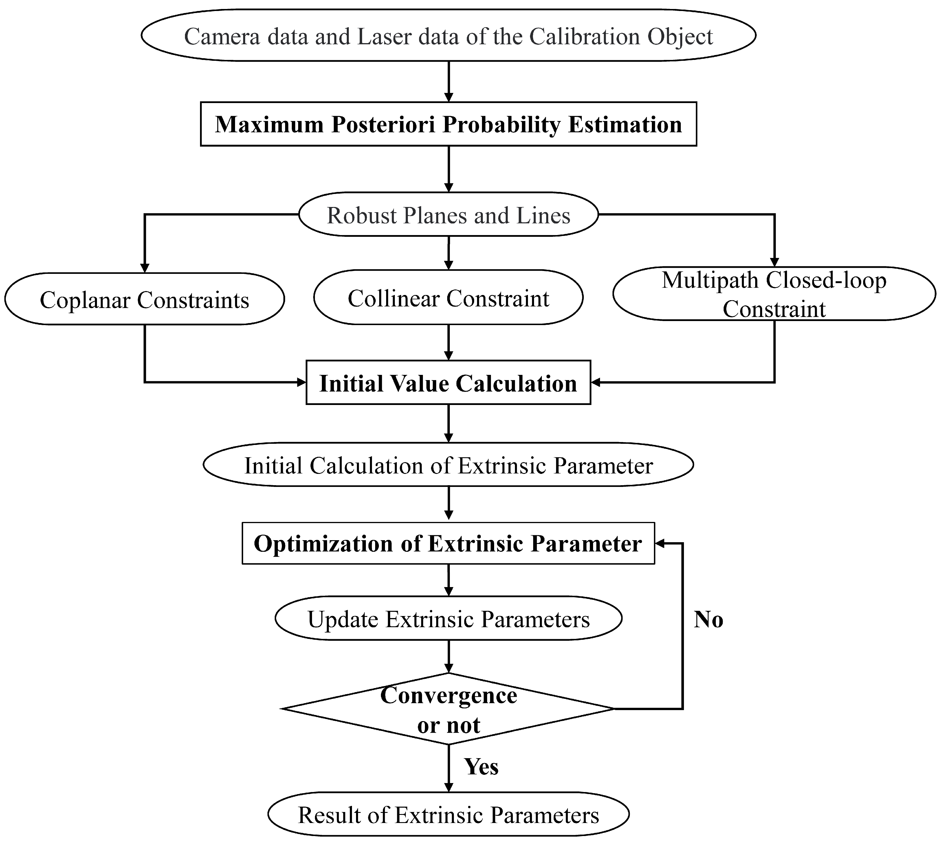
2.3. Multipath-Closure Calibration Process

As shown in Figure 7, the camera–LiDAR–camera multipath-closure calibration process consists of four steps. Firstly, the robust and accurate line and surface geometric information of the calibration object can be derived through the iterative maximum a posterior probability estimation. Secondly, coplanar constraints, collinear constraints, and multipath-closure constraints can be constructed based on the calibration targets and the multipath-closure interconnection between sensors. Subsequently, the initial values of the extrinsic parameters are obtained according to the coplanar and collinear constraints. Finally, using the L-M algorithm to optimize the initial values of the extrinsic parameters iteratively, the results of the extrinsic calibration can be obtained.

2.3.1. Initial Calculation of Extrinsic Parameters

Utilizing the random sample consensus (RANSAC) algorithm, the three checkerboard plane parameters $\left[{\mathit{n}}_i^L,d_i^L\right]$ and the three plane intersection line segment parameters $\left[{\mathit{l}}_i^L,{\mathit{Q}}^L\right]$ in the LiDAR point cloud are derived, where ${\mathit{Q}}^L$ is the intersection point of the three line segments. Subsequently, following Zhang’s method [41], the checkerboard plane parameters $\left[{\mathit{n}}_i^C,d_i^C\right]$ and the plane intersection line segment parameters $\left[{\mathit{l}}_i^C,{\mathit{Q}}^C\right]$ can be determined from the image data, along with the extrinsic parameters between the two cameras. According to Equation (5), for a single pose of the calibration object, the initial value of the translation vector can be written as

$${\mathit{T}}_L^C={\left[{\left({\mathit{n}}_1^C\right)}^T,{\left({\mathit{n}}_2^C\right)}^T,{\left({\mathit{n}}_3^C\right)}^T\right]}^{-1}\left[d_1^L-d_1^C,d_2^L-d_2^C,d_3^L-d_3^C\right]$$

(27)

In the case of multiple poses, an error function can be formulated regarding the translation vector ${\mathit{T}}_L^C$:

$${\mathit{T}}_L^C=\underset{{\mathit{T}}_L^C}{argmin}\sum _{i=1}^N\sum _{j=1}^3{\left({\left({\mathit{n}}_{ij}^C\right)}^T{\mathit{T}}_L^C-d_{ij}^L+d_{ij}^C\right)}^2$$

(28)

Let

$$\begin{array}{cc}\hfill {\mathit{N}}_C& =\left[{\left({\mathit{n}}_{11}^C\right)}^T,{\left({\mathit{n}}_{12}^C\right)}^T,{\left({\mathit{n}}_{13}^C\right)}^T,\dots \right]\hfill \end{array}$$

(29a)

$$\begin{array}{cc}\hfill {\mathit{D}}_C-{\mathit{D}}_L& =\left[d_{11}^L-d_{11}^C,d_{12}^L-d_{12}^C,d_{13}^L-d_{13}^C,\dots \right]\hfill \end{array}$$

(29b)

Due to the least squares method, the optimal solution of Equation (28) can be expressed as

$${\mathit{T}}_L^C={\left({\mathit{N}}_C{\mathit{N}}_C^T\right)}^{-1}{\mathit{N}}_C\left({\mathit{D}}_C-{\mathit{D}}_L\right)$$

(30)

Regarding the initial calculation of rotation indexes, the error function for the rotation matrix ${\mathit{R}}_L^C$ concerning a single pose data from Equations (4) and (9) is

$${\mathit{R}}_L^C=\underset{{\mathit{R}}_L^C}{argmin}\sum _{i=1}^3{\left({\mathit{R}}_L^C{\mathit{n}}_i^L-{\mathit{n}}_i^C\right)}^2+{\left({\mathit{R}}_L^C{\mathit{l}}_i^L-{\mathit{l}}_i^C\right)}^2$$

(31)

Let

$$\begin{array}{cc}\hfill {\mathit{M}}_L& =\left[{\mathit{n}}_1^L,{\mathit{n}}_2^L,{\mathit{n}}_3^L,{\mathit{l}}_1^L,{\mathit{l}}_2^L,{\mathit{l}}_3^L\right]\hfill \end{array}$$

(32a)

$$\begin{array}{cc}\hfill {\mathit{M}}_C& =\left[{\mathit{n}}_1^C,{\mathit{n}}_2^C,{\mathit{n}}_3^C,{\mathit{l}}_1^C,{\mathit{l}}_2^C,{\mathit{l}}_3^C\right]\hfill \end{array}$$

(32b)

According to [42], applying the SVD decomposition to the matrix ${\mathit{M}}_L{\mathit{M}}_C^T$, the result is ${\mathit{M}}_L{\mathit{M}}_C^T=\mathit{U}\mathit{S}{\mathit{V}}^T$, where the initial rotation matrix ${\mathit{R}}_L^C=\mathit{V}{\mathit{U}}^T$. The methodology to calculate the initial data values for multiple poses is mainly consistent with that used for a single pose.

2.3.2. Optimization of Extrinsic Parameters

Upon ensuring the initial values for the extrinsic parameters between the two cameras through LiDAR measurements, it is necessary to further optimize the initial values. Due to the coplanarity, covariance, and multipath-closure constraints, an error function for the extrinsic parameters can be derived and iteratively optimized to obtain a more precise result. Based on the error adjustment term of the coplanar constraints, collinear constraints, and multipath-closure constraint, the total optimization function can be written as

$$\left({\mathit{R}}_L^{C_1},{\mathit{T}}_L^{C_1},{\mathit{R}}_L^{C_2},{\mathit{T}}_L^{C_2}\right)=\underset{{\mathit{R}}_L^C,{\mathit{T}}_L^C}{argmin}{e}_{plane\_new}+e_{line}+e_{loop}$$

(33)

The Equation (33) solution presents a non-linear optimization problem that can be addressed through the L-M algorithm, which performs a global optimization of the extrinsic parameters.

3. Experimental Results and Analysis

In order to verify the effectiveness of the calibration algorithm in practical applications, this paper uses a sensor system composed of a stereo camera and a 3D LiDAR to collect data in multiple poses of the trihedron calibration object for actual experiments. Due to the lack of truth value for the extrinsic parameters in the actual experiment and the absence of the universally accepted accuracy evaluation standard, this paper proposes two accuracy indexes based on the correspondence of geometric features such as lines and planes in the image and point cloud data. One of the indexes is the overlap ratio, which calculates the area overlap ratio between the area of the calibration object in the LiDAR point cloud back-projected into the image and the actual area of the trihedron calibration object in the image (as shown in Figure 8); the calculation method is as follows:

$$IoU=\frac{S_L\cap S_C}{S_L\cup S_C}$$

(34)

where $\mathit{IoU}$ represents the overlap ratio, ${\mathit{S}}_{\mathit{C}}$ is the area of the calibration object in the image, and ${\mathit{S}}_{\mathit{L}}$ is the area of the region in the image that corresponds to the calibration object’s back-projected LiDAR point cloud. Assuming the extrinsic parameter results are accurate, the area of the LiDAR point cloud back-projected on the image is just covering the calibration object area in the image, so the accuracy of the algorithm can be evaluated by the overlap ratio, and the higher the overlap ratio, the higher the accuracy of the algorithm.

Another evaluation index is the line distance, which refers to the sum of the distance between the three planar intersection lines of the trihedron calibration object in the LiDAR point cloud back-projected into the image and the corresponding three intersection lines of the trihedron in the image (as illustrated in Figure 9); the calculation process can be written as

$$\begin{array}{cc}\hfill L& =\sum _{i=1}^3{\omega }_i{L}_i\hfill \end{array}$$

(35a)

$$\begin{array}{cc}\hfill L_i=∥{\mathit{Q}}_C^i-{\mathit{Q}}_L^i,∥& {\omega }_i=\left(1-∥{\mathit{l}}_{\mathbf{C}}^{\mathbf{i}}•{\mathit{l}}_{\mathit{l}}^{\mathbf{i}}∥\right)\hfill \end{array}$$

(35b)

In Equation (35), $\left[{\mathit{l}}_{\mathbf{C}}^{\mathit{i}},{\mathit{Q}}_C^i\right],(i=1,2,3)$ represents the parameter of the intersection lines of the three trihedron calibration objects in the image obtained by the back projection and $\left[{\mathit{l}}_{\mathit{l}}^{\mathit{i}},{\mathit{Q}}_L^{\mathit{i}}\right],(i=1,2,3)$ denotes the parameters of the intersecting planes of the trihedron calibration object in the LiDAR point cloud. L is the line distance. The more accurate the calibration result is, the closer the values of ${!}_{\mathit{i}}$ and ${\mathit{L}}_{\mathit{i}}$ in Equation (35) approach 0, and the resulting line distance calculation also approaches 0. Therefore, the line distance can also evaluate the algorithm’s accuracy; the smaller the line distance, the higher the accuracy of the algorithm.

Based on real experiments, this paper uses two evaluation indexes, overlap ratio and line distance, to validate the accuracy of the algorithm in real scenarios and evaluate the impact of different constraints on the calibration results from both planar and linear perspectives.

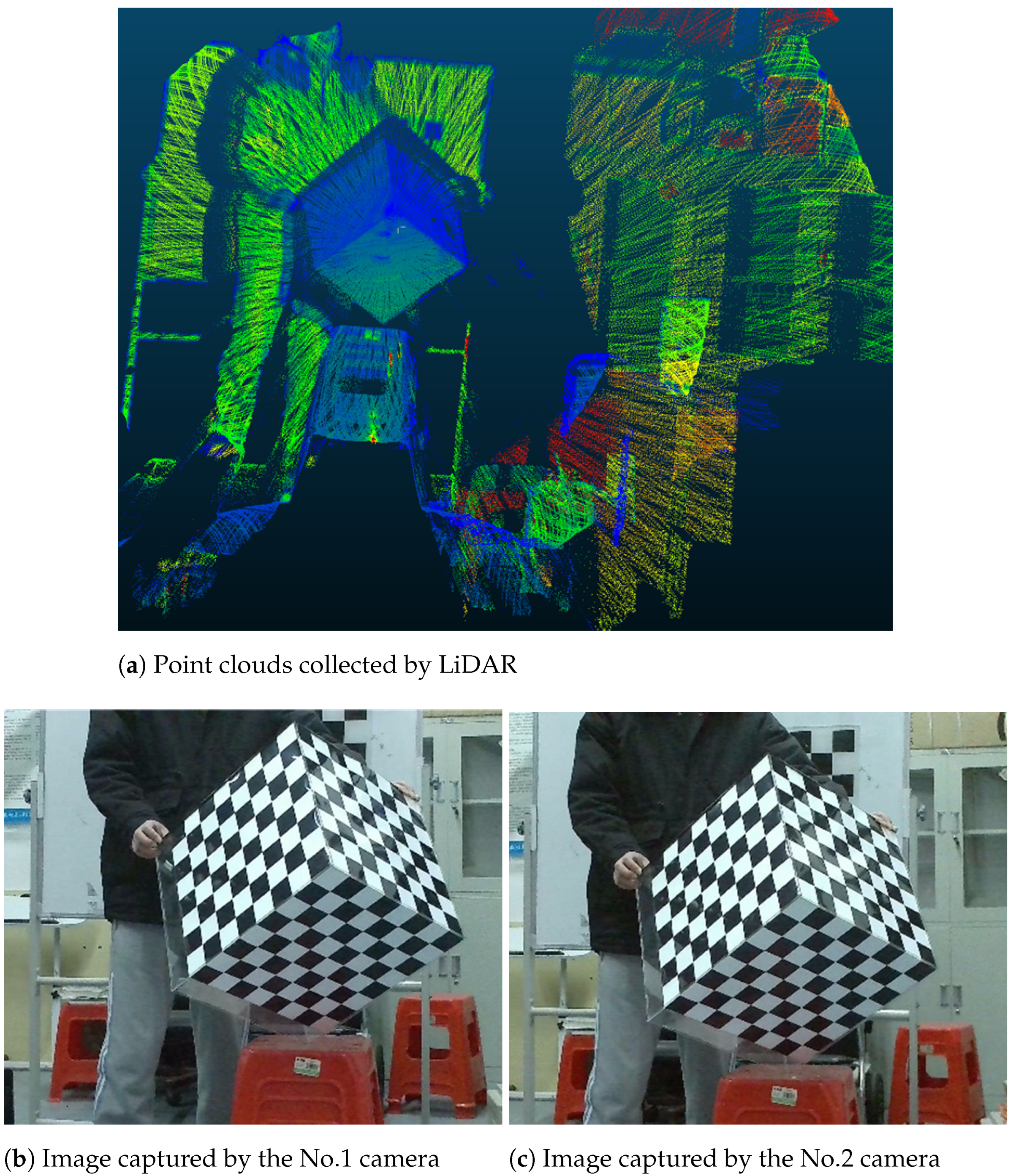
3.1. Real Experiments

In order to verify the effectiveness of the calibration algorithm proposed in this paper in real-world scenarios, this paper uses real data collected by a sensor system composed of a stereo camera module and a 3D LiDAR; the equipment diagram is shown in Figure 10.

The equipment in the experiment consists of two cameras and a 3D LiDAR with the following parameters: a focal length of 28 mm, a principal point coordinate of (972, 485), the resolution of the image acquired by the camera is 1920 × 1080, and the aberration parameters are [0.056,−0.9972,−0.001,0.00014,−17.107]. The 3D LiDAR parameters are shown in

Table 1. 3D LiDAR parameters.

Vertical Field of View	90 degrees
Vertical Angle Resolution	1 degree
Horizontal Field of View	270 degrees
Horizontal Angle Resolution	0.5 degrees

.

Three checkerboard grids were used for the trihedron calibration object; each checkerboard grid was 8 × 8 grids with a size of 50 mm, and the size of each checkerboard grid was 40 cm × 40 cm. The internal camera parameters, such as the focal length, principal point coordinate, and aberration parameters, were calibrated before the experiment. The images taken by the cameras were corrected for aberration during the experiment. The baseline of the stereo camera in the experimental equipment was adjustable, and the experimental results under different baselines are basically consistent without loss of generality. This paper sets the baseline length as approximately 10 cm in the experiment. The data collected by the experimental equipment is illustrated in Figure 11.

3.1.1. Accuracy Verification of Algorithms in Real Scenarios

In the experiment, the relative position of the LiDAR and stereo camera was fixed, and the calibration object was moved to collect data under 20 different poses. This paper implements the verification algorithm to derive the extrinsic parameters of the LiDAR and stereo camera, which can be written as

$$\begin{array}{cc}\hfill {\mathit{R}}_L^{C_1}& =\left[\begin{array}{ccc}0.078& -0.992& -0.011\\ -0.043& -0.013& -0.993\\ 0.996& 0.083& -0.044\end{array}\right]\hfill \end{array}$$

(36a)

$$\begin{array}{cc}\hfill {\mathit{T}}_L^{C_1}& =[12.175\mathrm{mm},142.101\mathrm{mm},170.953\mathrm{mm}]\hfill \end{array}$$

(36b)

$$\begin{array}{cc}\hfill {\mathit{R}}_L^{C_2}& =\left[\begin{array}{ccc}0.081& -0.995& -0.005\\ -0.042& -0.0& -0.992\\ 0.995& 0.087& -0.042\end{array}\right]\hfill \end{array}$$

(36c)

$$\begin{array}{cc}\hfill {\mathit{T}}_L^{C_2}& =[-83.650\mathrm{mm},136.259\mathrm{mm},172.603\mathrm{mm}]\hfill \end{array}$$

(36d)

Based on the obtained extrinsic calibration results, the calibration object regions of the LiDAR point cloud were respectively back-projected onto the No.1 camera and the No.2 camera. The back-projection results are shown in Figure 12.

In Figure 12, the red dots indicate the LiDAR points, and the overlap ratio calculated by Equation (34) is 0.93 for the No.1 camera and 0.91 for the No.2 camera. From the two back-projection images, it can be observed that the LiDAR points of the trihedron calibration object acquired by the LiDAR are distributed in the calibration area of the image after the back-projection transformation, and they basically cover the region. Moreover, the LiDAR points on each checkerboard plane in the image are distributed almost uniformly. In addition to the back projection of the entire calibration region, this paper back-projects the intersection of the trihedron calibration object in the point cloud to the image based on the extrinsic parameter calibration results, as shown in Figure 13.

In Figure 13, the red dots represent LiDAR points, and the line distance calculated by Equation (35) is 0.96 for the No.1 camera and 0.94 for the No.2 camera. From the two back-projection images, it can be observed that the back-projection lines of the calibration plane intersection in the LiDAR point cloud almost coincide with the intersection line of the calibration plane in the image. Based on the results illustrated in Figure 12 and Figure 13, it can be concluded that the extrinsic calibration obtained by the proposed algorithm in this paper matches the pose of the stereo camera and the 3D LiDAR during operation in the real scene, indicating the accuracy of the proposed algorithm in this paper.

3.1.2. Influence of Point Cloud Noise Estimation Methods on the Calibration Results

The primary objective of estimating point cloud noise is to obtain robust and accurate coplanar constraint relationships. In order to verify the impact of point cloud noise estimation methods on calibration results, we employed the same experimental data as in Section 3 to calculate the extrinsic parameters under two cases of coplanar constraint with estimation and coplanar constraint without noise estimation; the back-projection results (the No.1 camera) are shown in Figure 14.

From Figure 14, it can be seen that, without noise estimation, the back projection of the checkerboard plane in the point cloud onto the image does not correspond well with the checkerboard plane in the image, and the intersection lines of the checkerboard in the point cloud and those in the image show significant deviations. Therefore, it can be deduced that ensuring a robust and accurate coplanar constraint relationship through noise estimation can yield more precise calibration results.

3.1.3. Influence of Different Constraints on Calibration Results

In order to investigate the influence of different constraints on the calibration results and compare them with existing methods, we employed the same experimental data as in Section 3 to calculate the extrinsic parameters under three cases: coplanar constraint, coplanar constraint + collinear constraint, and coplanar constraint + multipath-closure constraint + collinear constraint. The extrinsic parameters were compared with the results obtained by the method proposed in the literature [14]. Calculating the accuracy indexes according to the back-projection test and Equations (34) and (35), the results are presented in

Table 2. Results of precision indexes calculation.

Constraints Condition	Overlap Ratio	Line Distance
Literature [14]	0.67	9.33
Coplanar	0.85	2.31
Coplanar + Collinear	0.88	1.04
Coplanar + Multipath-closure + Collinear	0.93	0.95

.

From the results of the back-projection and overlap ratio calculation, it can be summarized that (1) the precision of the algorithm presented in this paper is significantly higher than that of existing methods, primarily because existing methods only utilize a single coplanar constraint, whereas our algorithm combines multiple constraint relationships and improves their accuracy through noise estimation; (2) both the multipath-closure and the collinear constraints can improve the algorithm’s precision, with the multipath-closure constraint resulting in a more significant improvement in the overlap ratio index, while the collinear constraint result in a greater improvement in the line distance index. The experimental results demonstrate that more accurate calibration results can be obtained under the combined effect of various constraints such as coplanarity, collinearity, and multipath-closure constraints.

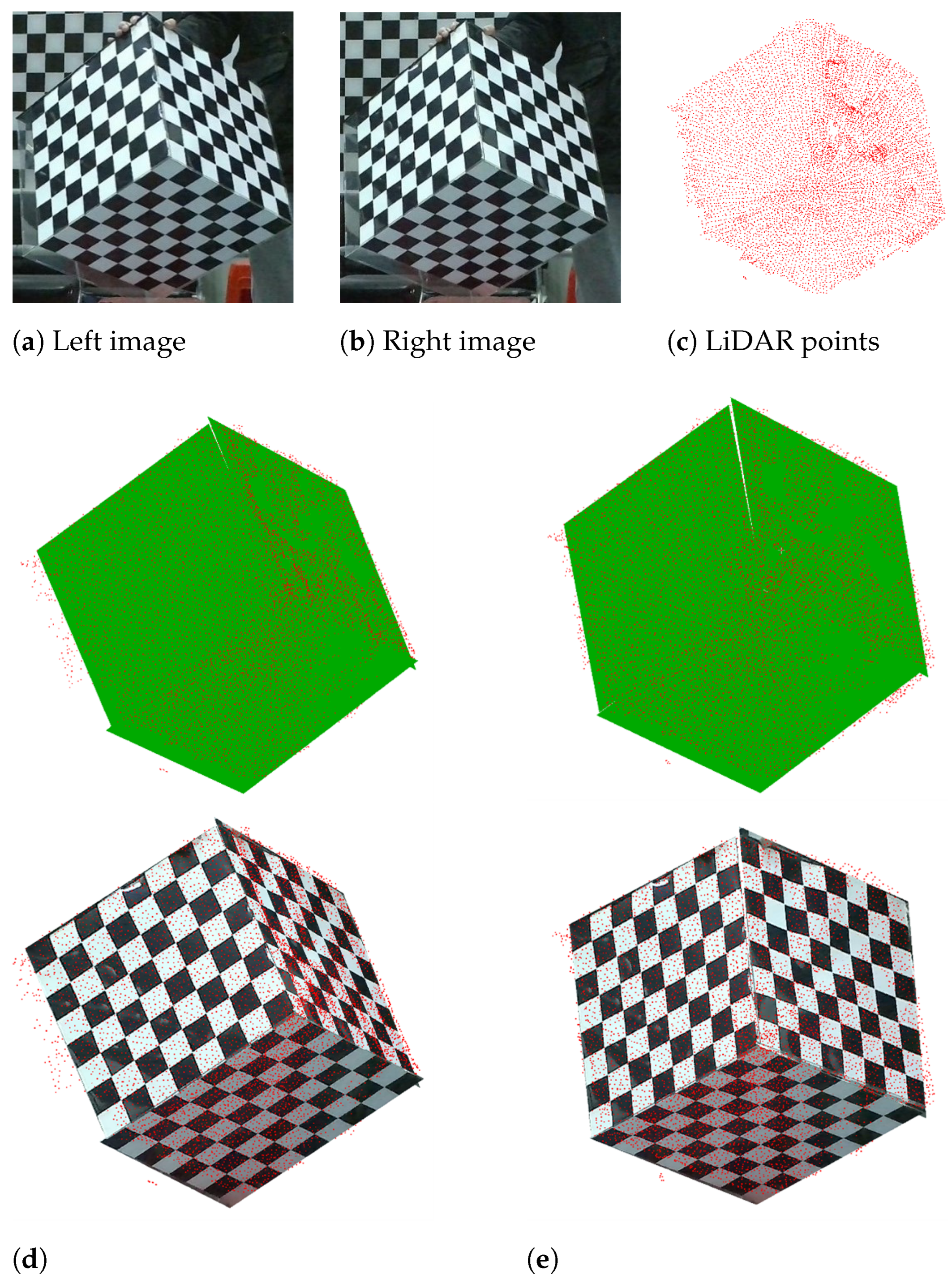
3.1.4. Data Fusion Results Using the Calibration Results

Calibration results are primarily used for data fusion between sensors, including data fusion between images and data fusion between images and point clouds.

(1) Data Fusion between Images and Point Clouds

LiDAR point clouds are sparse, unordered, and lack texture information. By utilizing the extrinsic parameters between the camera and the LiDAR, the color texture information in the images can be mapped onto the point clouds, resulting in a more comprehensive and rich scene information. In this paper, the color texture information from the image data collected by the experimental equipment is mapped onto the point cloud data, and the resulting data fusion result is shown in Figure 15a.

In order to validate the accuracy of the data fusion results, we measured the size of the calibration object’s checkerboard grid in the point cloud using the CloudCompare software (2.12.4 Kyiv [Windows 64-bit]). The result is shown in Figure 15b.

Figure 15b is an enlarged view of the calibration object region in Figure 15a. Through the measurement tool in CloudCompare, the width of four checkerboard grid cells in the point cloud is approximately 0.196 m, which means that the size of each checkerboard grid cell is approximately 49 mm. The actual size of the checkerboard grid cell is 50 mm. The experimental result is very close to the true value, demonstrating the accuracy of the fusion results.

(2) Data Fusion between Images

Based on the extrinsic parameters between stereo cameras, the three-dimensional point cloud of the scene can be reconstructed from the images of the stereo cameras. The reconstruction methods can be broadly categorized into disparity-based and feature matching-based approaches. The feature matching-based approach is suitable for simple scenes composed of multiple planes and provides more accurate depth estimation. The disparity-based approach has a wider range of applications but less accurate depth estimation compared to the feature matching-based approach. However, the prerequisite for the disparity-based approach is that the optical axes of the two cameras are parallel, meaning that the images captured by the two cameras only have a certain pixel offset in the horizontal direction. In this study, the intrinsic parameters of the stereo cameras in the experimental equipment are not completely consistent, and the captured images have pixel offsets in both the horizontal and vertical directions, which does not meet the conditions for using the disparity-based approach. Therefore, the feature matching method is adopted for three-dimensional reconstruction. Firstly, feature extraction and matching are performed on the images from the left and right cameras to obtain corresponding feature points. Then, the depth values of the corresponding feature points are estimated based on the extrinsic parameters between the cameras, resulting in three-dimensional points corresponding to the feature points in the spatial domain. Finally, dense reconstruction is performed to obtain the reconstruction results, as shown in Figure 16.

As shown in Figure 16, this paper reconstructed the trihedron calibration object using both the left camera coordinate system and the right camera coordinate system as references. The size of the checkerboard grid in the reconstructed point cloud was measured, resulting in dimensions of 51.7 mm and 50.8 mm, respectively. These values are close to the true size, demonstrating the accuracy of the reconstruction results. Furthermore, this paper also fused the point cloud reconstructed from images with the point cloud from a LiDAR. By using the extrinsic parameters between the left and right cameras and the LiDAR, the point cloud reconstructed from images was projected onto the LiDAR coordinate system. The LiDAR point cloud was then densified. From the projection results in Figure 16, it can be observed that the point clouds of the tetrahedron calibration object reconstructed using both the left and right cameras align well with the corresponding region in the LiDAR point cloud, indicating good fusion results.

3.2. Simulation Experiments

However, the actual experiments have the following limitations: (1) precisely measuring the algorithm’s accuracy takes a significant amount of work. In actual experiments, the truth values of the extrinsic parameters are unknown. The accuracy of the calibration algorithm can only be roughly evaluated by the correspondence between the lines and surfaces after the point cloud back projection and the lines and surfaces in the image; (2) Noise and limited pose conditions make it difficult to measure the algorithm’s robustness. The equipment used in actual experiments is fixed. Meanwhile, the noise conditions and pose range in the collected data are limited, making it impossible to obtain the algorithm performance under different noise conditions and some special pose data. Therefore, this paper designs simulation experiments to quantitatively evaluate the performance of the calibration algorithm by simulating data under various noise conditions and special poses with known truth values of extrinsic parameters, and the performance evaluation indexes are as follows:

$$\left\{\begin{array}{c}{E}_R=2cos\left(\frac{tr\left(R_{cali}^{-1}{R}_{truth}-I\right)}{2}\right)\\ E_T=\Vert T_{truth}-T_{cali}\Vert \end{array}\right.$$

(37)

In Equation (37), $\left[{\mathit{R}}_{cali},{\mathit{T}}_{cali}\right]$ is the output extrinsic parameter of the algorithm and $\left[{\mathit{R}}_{truth},{\mathit{T}}_{truth}\right]$ is the extrinsic truth value. This evaluation index allows for a quantitative assessment of the differences between the truth value and the algorithmic output, and the smaller the calculated result, the better the performance of the algorithm.

To ensure that the results of the simulation experiments closely reflect real-world scenarios, the parameter settings of the simulation experiment are set to match those of the real-world scenarios as closely as possible.

Specifically, the parameters of the 3D LiDAR and the calibration object in the simulation experiment are consistent with those of the real experiment, the aberration parameter of the camera is set to 0, and the other parameters are also consistent with the real experiment.

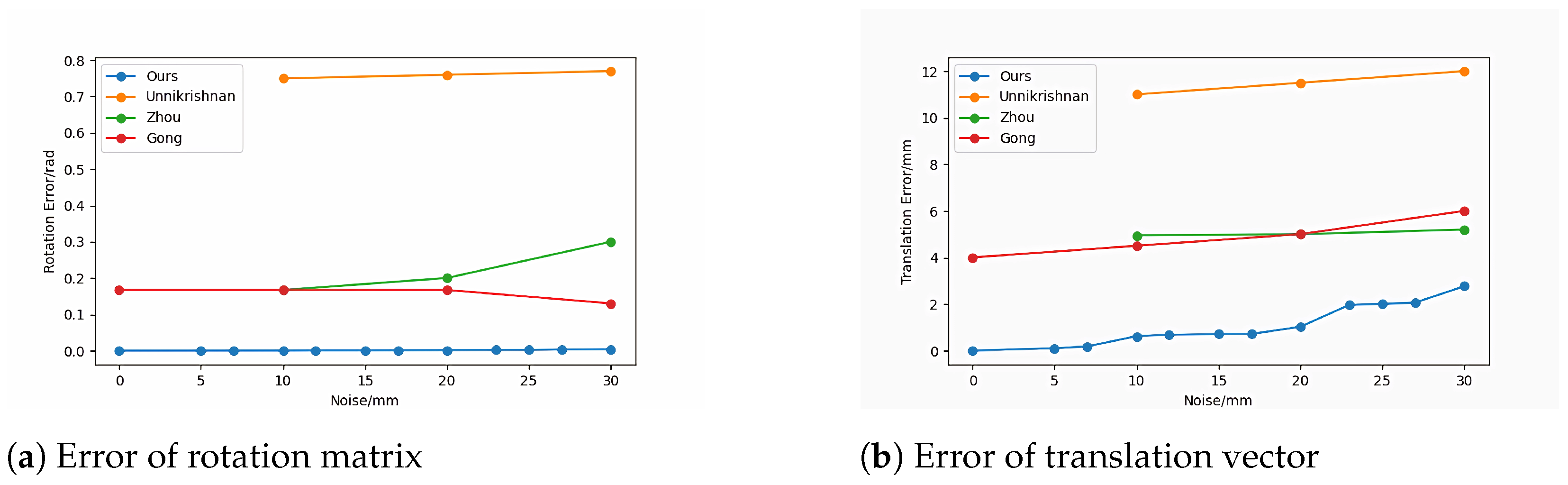
3.2.1. Simulation Experiments under Different LiDAR Noise

To verify the adaptability of the algorithm to LiDAR noise, Gaussian noise with a mean of 0 and a standard deviation of 2–30 mm was added to the LiDAR distance data and Gaussian noise with a mean value of 0 and standard deviation of 0.5 pixels was added to the image point data. Fifty experiments were conducted at each noise level, and in each experiment the simulation generated data for a trihedron calibration object in one pose. The calibration algorithm proposed in this paper was used to calculate the extrinsic parameters, and the accuracy of the algorithm was calculated using Equation (37). The accuracy comparison results with the current mainstream methods (Unnikrishnan [8], Zhou [14], Toth [43]) are shown in Figure 17.

The results of the extrinsic calibration error between the LiDAR and Camera No.2 at different levels of LiDAR noise are similar to those shown in Figure 17. According to Figure 17, it can be summarized that with the increase of the LiDAR noise, the calibration errors of the rotation matrix and the translation vector would gradually increase. However, even when the noise parameter is increased to 30 mm, the error of the rotation matrix remains within 0.004 rad and the error of the translation vector remains within 4 mm. This proves that this paper’s algorithm has good accuracy and robustness under the data of the trihedron calibration object with a single pose. Moreover, compared to the current mainstream methods, this paper combines multiple constraint relationships and enhances their accuracy and robustness through noise estimation. As a result, more accurate extrinsic calibration results are obtained.

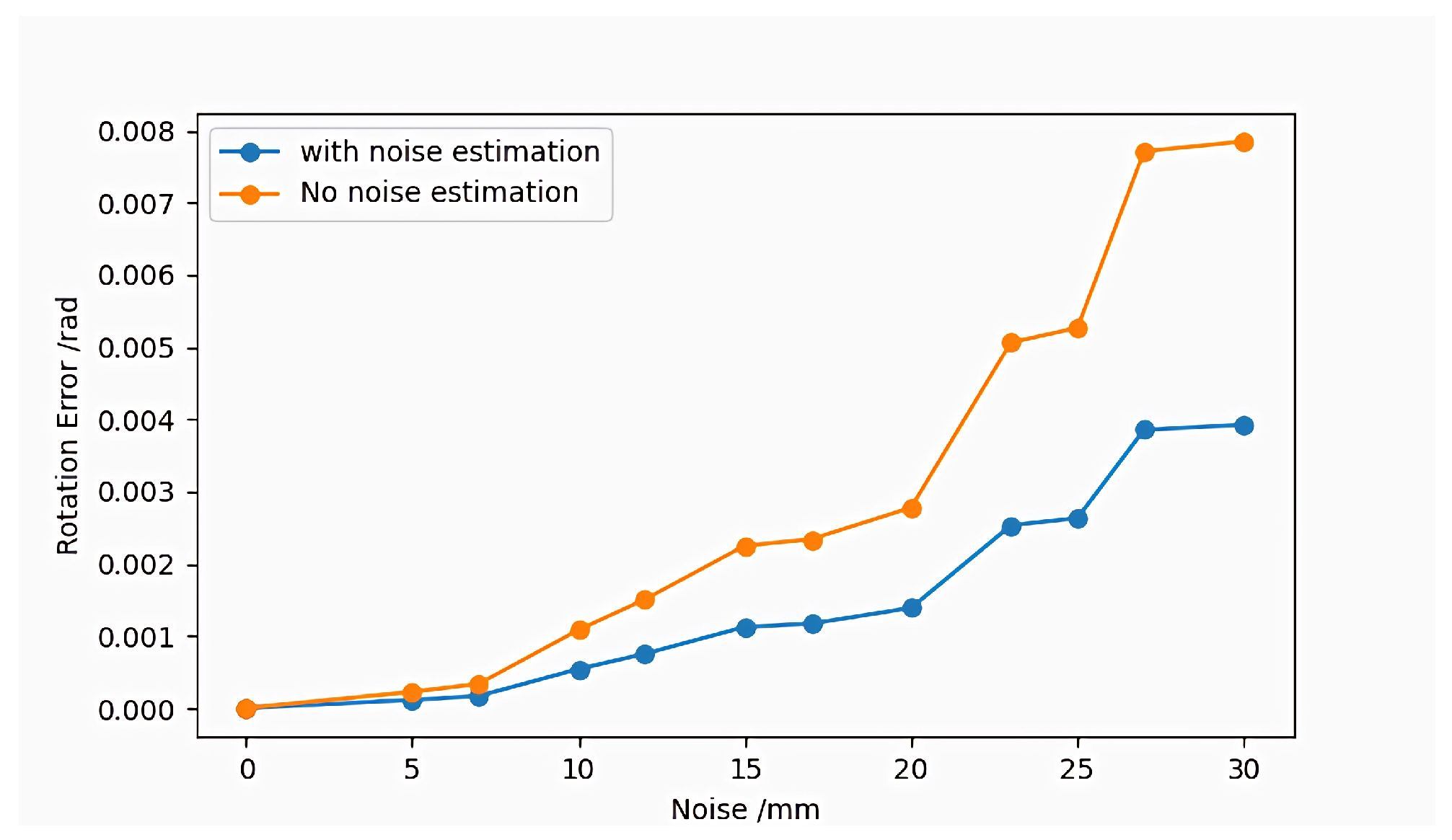
3.2.2. Influence of Point Cloud Noise Estimation Methods on Algorithm Accuracy

The main purpose of point cloud noise estimation is to obtain robust and accurate coplanar constraints. In order to verify the influence of the point cloud noise estimation methods on algorithm accuracy, this paper introduces Gaussian noise with a mean of 0 and standard deviation of 20 mm into the LiDAR data and conducts 50 experiments at this noise level. In each experiment, the simulation generates data from the trihedron calibration object with one pose. The extrinsic parameters were calculated for coplanar constraint and coplanar constraint without noise estimation, the algorithmic accuracy was calculated from Equation (34), and the result is presented in Figure 18.

As depicted in Figure 18, it is evident that, in the absence of noise estimation, the calibration error is significantly larger. However, the robust and accurate coplanar constraint obtained from noise estimation can improve the precision of calibration.

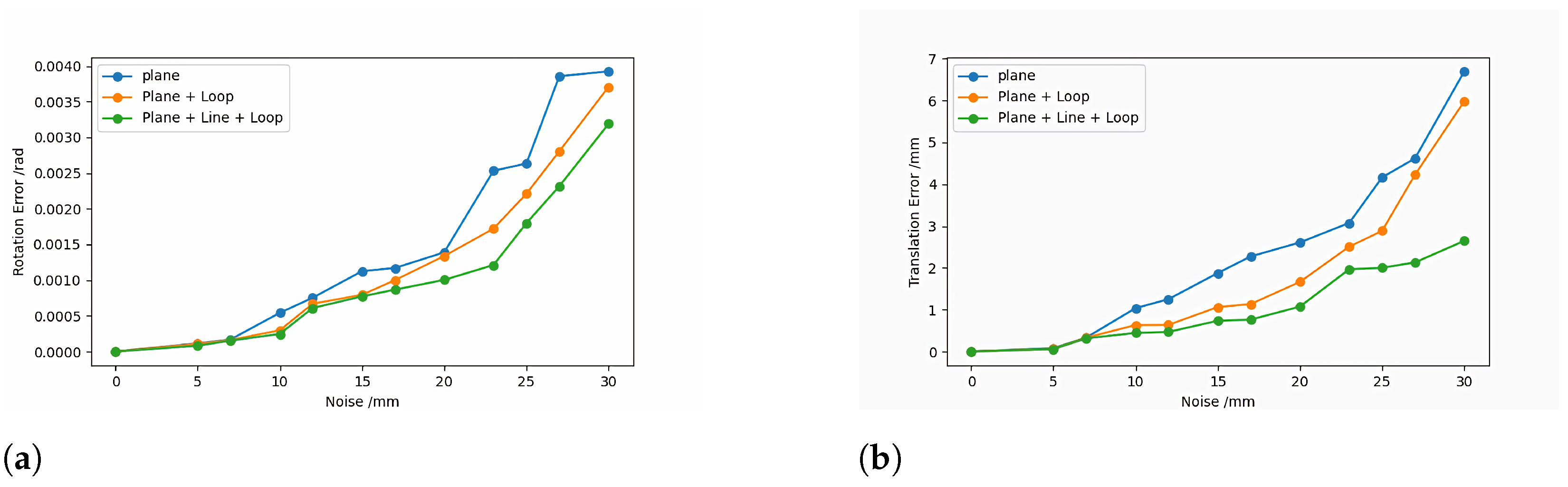
3.2.3. Influence of Coplanar Constraint and Multipath-Closure Constraint on Algorithm’s Accuracy

In this paper, the algorithm adds collinear and multipath-closure constraints on the basis of coplanar constraints, and in order to verify the influence of coplanar and loop constraints on the algorithm’s accuracy this paper adds Gaussian noise with a mean value of 0 and standard deviation of 20 mm to the LiDAR data. Fifty experiments were conducted at this noise level, with each experiment generating data for the trihedron calibration object under one pose. The extrinsic parameters were computed under three conditions: coplanar constraint only, coplanar constraint + loop constraint, and coplanar + loop + collinear constraints. The accuracy of the algorithm was calculated using Equation (37), and the results are shown in Figure 19 and Figure 20.

As shown in Figure 19 and Figure 20, it is evident that the loop and collinear constraints can enhance calibration algorithm’s accuracy. The combined effect of the loop constraint and the collinear constraint improves the calibration accuracy of the translation vector by nearly 50% compared with no loop or collinear.

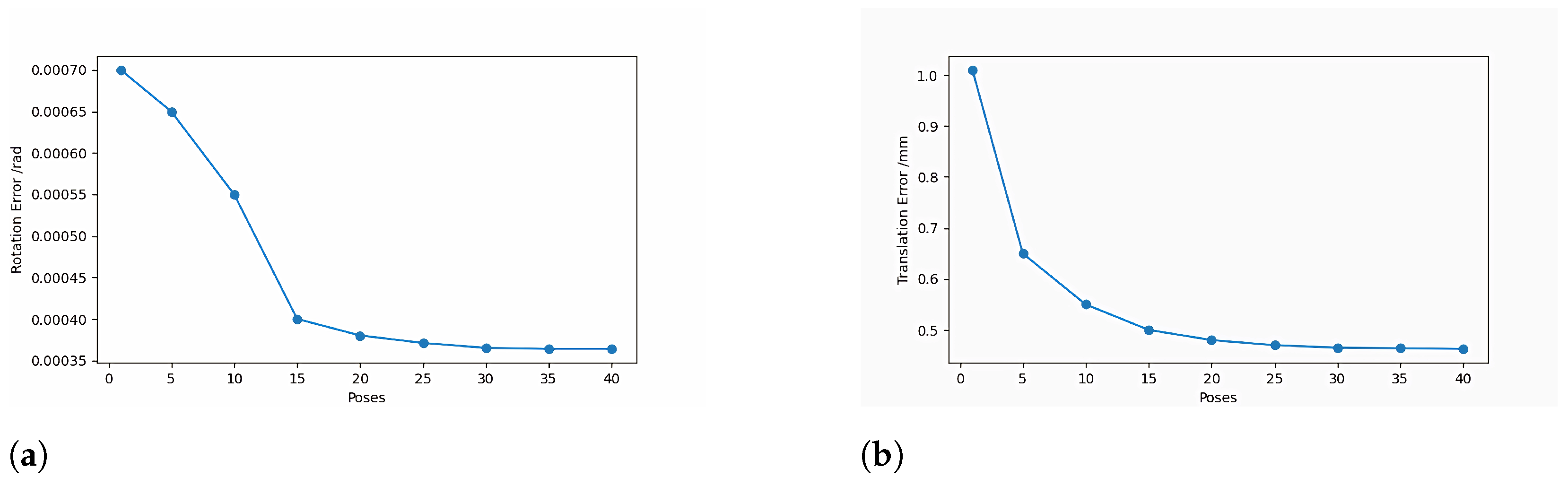
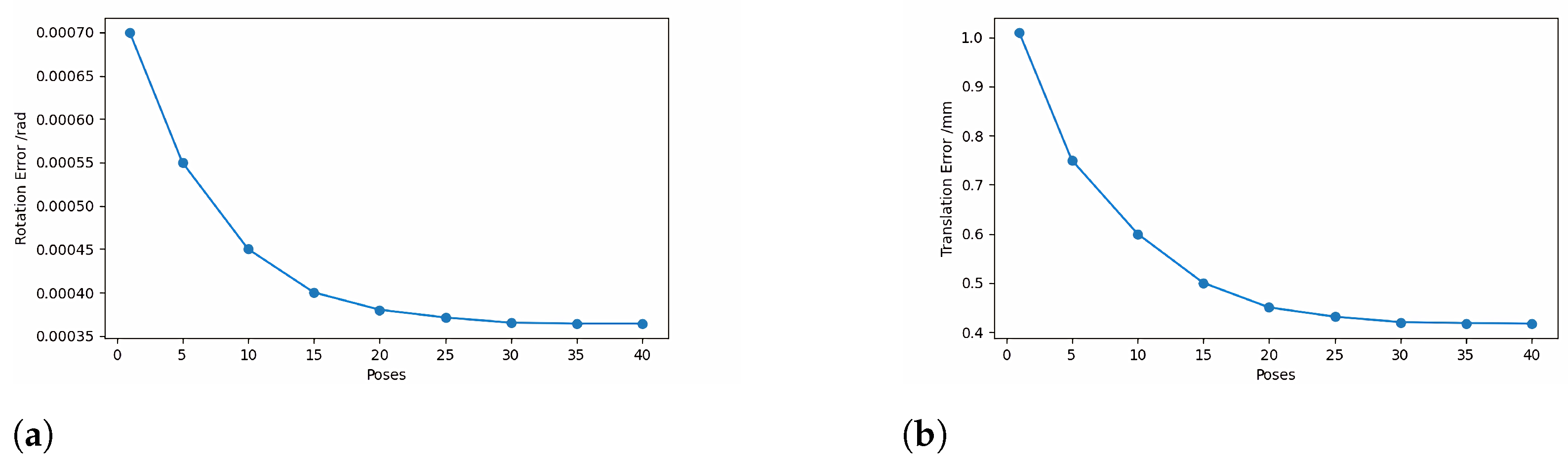
3.2.4. Influence of The Trihedron Calibration Object Poses Number on The Algorithm’s Accuracy

The calibration algorithm in this paper can work effectively for a single pose, but in practice, data are usually collected for multiple poses to improve the calibration accuracy. In order to verify the effect of the number of poses on the accuracy of the algorithm, this paper adds Gaussian noise with the mean value 0 and the standard deviation 20 mm to the LiDAR data. Fifty experiments were conducted at this noise level, with each experiment simulating 2 to 40 poses of the trihedron calibration object. The extrinsic calibration was performed using data from multiple poses, and the algorithm accuracy was calculated through the Equation (37). The results are presented in Figure 21 and Figure 22.

As depicted in Figure 21 and Figure 22, it is clear that the increase of the pose data can enhance the calibration accuracy of the algorithm. Once the number of poses reaches about 35, the accuracy gradually converges and no longer decreases. Ultimately, the converged accuracy data is nearly 50% higher than that obtained from a single pose.

4. Discussion

4.1. Accuracy Comparison between the Proposed Method and the Current Mainstream Methods

This paper compares the proposed method with the current mainstream methods in simulation experiments. The comparison results are presented in Figure 17. In the same simulated environment, the proposed method exhibits superior calibration accuracy compared to the current mainstream methods.

4.2. Influence of Point Cloud Noise Estimation Methods on the Calibration Results

To validate the effectiveness of the point cloud noise estimation method, this paper compares the calibration results under two scenarios: without noise estimation and with noise estimation, in both simulation and real experiments. The results of the real experiment are shown in Figure 14, where without noise estimation the back-projected chessboard planes from the point cloud do not align well with the corresponding image chessboard planes. Moreover, there is significant deviation between the chessboard intersections in the point cloud and the image. However, with noise estimation the back-projection results are improved. The results of the simulation experiment, shown in Figure 18, indicate that calibration accuracy is better with noise estimation compared to without. Both the simulation and real experiment results demonstrate that robust and accurate coplanar constraints obtained through noise estimation can enhance the precision of calibration.

4.3. Influence of Different Constraints on Calibration Results

To validate the effectiveness of coplanar constraints and multipath-closure constraints, this paper compares the calibration results under three scenarios: coplanar constraints, coplanar constraints + collinear constraints, and coplanar constraints + collinear constraints + multipath-closure constraints, in both simulation and real experiments. The results of the real experiment are presented in Table 2, indicating that both multipath-closure constraints and collinear constraints improve the algorithm’s accuracy measures. multipath-closure constraints exhibit greater improvement in the overlap metric, while collinear constraints show greater improvement in the online distance metric. The results of the simulation experiment, shown in Figure 19, demonstrate that both multipath-closure and collinear constraints enhance the calibration algorithm’s accuracy. In fact, the combined effect of multipath-closure and collinear constraints improves the translational vector calibration accuracy by nearly half compared to the absence of multipath-closure and collinear constraints. The experimental results indicate that more accurate calibration results can be achieved through the combined effect of coplanar constraints, collinear constraints, and multipath-closure constraints.

5. Conclusions

This paper proposes a calibration method for a stereo camera and 3D LiDAR, which incorporates multiple constraints. The contributions can be summarized in three main points. Firstly, based on the plane established by the trihedron calibration object, a more precise extrinsic calibration is achieved by incorporating various geometric constraints such as coplanarity and collinearity. The geometric constraints established by the calibration object are crucial for the extrinsic calibration of the two sensors, and the more geometric constraints there are, the higher the accuracy of the extrinsic calibration. Secondly, the multipath-closure constraint is established through the multipath-closure interconnection between the three sensors to reduce the calibration errors and further improve the algorithm’s accuracy. Finally, two indexes, namely overlap ratio and line distance, are proposed to evaluate the accuracy of the extrinsic calibration in the actual data. The results of extrinsic calibration can be tested from the plane and line perspectives, respectively.

We have two main directions for our future research: (1) Advanced Calibration Methods. Here we will investigate and develop more advanced calibration methods that can further improve the accuracy and robustness of the extrinsic calibration process. This could involve exploring novel mathematical models, optimization algorithms, or incorporating additional sensor modalities. (2) Multi-Sensor Fusion for Practical Applications. Here we will explore the integration of a stereo camera and LiDAR data for multi-sensor fusion applications. This could involve developing algorithms for specific real-world applications such as autonomous driving and robotics.

References

1. Alismail, H.; Browning, B. Automatic calibration of spinning actuated lidar internal parameters. J. Field Robot. 2015, 32, 723–747. [Google Scholar] [CrossRef]
2. Bogue, R. Sensors for robotic perception. Part two: Positional and environmental awareness. Ind. Robot. Int. J. 2015, 42, 502–507. [Google Scholar] [CrossRef]
3. Du, L.; Zhang, T.; Dai, X. Robot kinematic parameters compensation by measuring distance error using laser tracker system. Infrared Laser Eng. 2015, 44, 2351–2357. [Google Scholar]
4. Xiao, R.; Xu, Y.; Hou, Z.; Chen, C.; Chen, S. An automatic calibration algorithm for laser vision sensor in robotic autonomous welding system. J. Intell. Manuf. 2022, 1–14. [Google Scholar] [CrossRef]
5. Xu, F.; Xu, Y.; Zhang, H.; Chen, S. Application of sensing technology in intelligent robotic arc welding: A review. J. Manuf. Process. 2022, 79, 854–880. [Google Scholar] [CrossRef]
6. Xie, D.; Chen, L.; Liu, L.; Chen, L.; Wang, H. Actuators and sensors for application in agricultural robots: A review. Machines 2022, 10, 913. [Google Scholar] [CrossRef]
7. Kang, H.; Wang, X.; Chen, C. Accurate fruit localisation using high resolution LiDAR-camera fusion and instance segmentation. Comput. Electron. Agric. 2022, 203, 107450. [Google Scholar] [CrossRef]
8. Yin, J.; Luo, D.; Yan, F.; Zhuang, Y. A novel lidar-assisted monocular visual SLAM framework for mobile robots in outdoor environments. IEEE Trans. Instrum. Meas. 2022, 71, 1–11. [Google Scholar] [CrossRef]
9. Zhang, Y.; Fanyu, L.Y.D.; Yan, X. Map-building approach based on laser and depth visual sensor fusion SLAM. Appl. Res. Comput. 2016, 33, 2970–2972. [Google Scholar]
10. Lenac, K.; Kitanov, A.; Cupec, R.; Petrović, I. Fast planar surface 3D SLAM using LIDAR. Robot. Auton. Syst. 2017, 92, 197–220. [Google Scholar] [CrossRef]
11. Ye, Y.; Fu, L.; Li, B. Object detection and tracking using multi-layer laser for autonomous urban driving. In Proceedings of the 19th IEEE International Conference on Intelligent Transportation Systems, Rio de Janeiro, Brazil, 1–4 November 2016. [Google Scholar]
12. Droeschel, D.; Schwarz, M.; Behnke, S. Continuous mapping and localization for autonomous navigation in rough terrain using a 3D laser scanner. Robot. Auton. Syst. 2017, 88, 104–115. [Google Scholar] [CrossRef]
13. Reichel, S.; Burke, J.; Pak, A.; Rentschler, T. Camera calibration as machine learning problem using dense phase shifting pattern, checkerboards, and different cameras. Opt. Data Sci. IV 2023, 12438, 185–197. [Google Scholar]
14. ElSheikh, A.; Abu-Nabah, B.A.; Hamdan, M.O.; Tian, G.-Y. Infrared Camera Geometric Calibration: A Review and a Precise Thermal Radiation Checkerboard Target. Sensors 2023, 23, 3479. [Google Scholar] [CrossRef] [PubMed]
15. Chen, B.; Liu, Y.; Xiong, C. Automatic checkerboard detection for robust camera calibration. In Proceedings of the 2021 IEEE International Conference on Multimedia and Expo (ICME), Shenzhen, China, 5–9 July 2021. [Google Scholar]
16. Gao, Z.; Zhu, M.; Yu, J. A self-identifying checkerboard-like pattern for camera calibration. In Proceedings of the 2020 39th Chinese Control Conference (CCC), Shenyang, China, 27–29 July 2020. [Google Scholar]
17. Gao, Z.; Zhu, M.; Yu, J. A novel camera calibration pattern robust to incomplete pattern projection. IEEE Sens. J. 2021, 21, 10051–10060. [Google Scholar] [CrossRef]
18. Juarez-Salazar, R.; Diaz-Ramirez, V.H. Flexible camera-projector calibration using superposed color checkerboards. Opt. Lasers Eng. 2019, 120, 59–65. [Google Scholar] [CrossRef]
19. Unnikrishnan, R.; Hebert, M. Fast Extrinsic Calibration of a Laser Rangefinder to a Camera (Tech. Report); CMU-RI-TR-05-09; Robotics Institute, Carnegie Mellon University: Pittsburgh, PA, USA, 2015. [Google Scholar]
20. Pandey, G.; McBride, J.; Savarese, S.; Eustice, R. Extrinsic calibration of a 3D laser scanner and an omnidirectional camera. Fac Proc. Vol. 2010, 43, 336–341. [Google Scholar] [CrossRef]
21. Mirzaei, F.M.; Kottas, D.G.; Roumeliotis, S.I. 3D LIDAR–camera intrinsic and extrinsic calibration: Identifiability and analytical least-squares-based initialization. Int. J. Robot. Res. 2012, 31, 452–467. [Google Scholar] [CrossRef]
22. Gong, X.; Lin, Y.; Liu, J. Extrinsic calibration of a 3D LIDAR and a camera using a trihedron. Opt. Lasers Eng. 2013, 51, 394–401. [Google Scholar] [CrossRef]
23. Khosravian, A.; Chin, T.; Reid, I. A branch-and-bound algorithm for checkerboard extraction in camera-laser calibration. arXiv Prepr. 2017, arXiv:1704.00887. [Google Scholar]
24. Zhou, L.; Deng, Z. Extrinsic calibration of a camera and a lidar based on decoupling the rotation from the translation. In Proceedings of the IEEE Intelligent Vehicles Symposium, Madrid, Spain, 3–7 June 2012. [Google Scholar]
25. Lu, R.; Wang, Z.; Zou, Z. Accurate Calibration of a Large Field of View Camera with Coplanar Constraint for Large-Scale Specular Three-Dimensional Profile Measurement. Sensors 2023, 23, 3464. [Google Scholar] [CrossRef]
26. Liu, W.; Zhang, Z.; Gu, Y.; Zhai, C. Fast and practical method for underwater stereo vision calibration based on ray-tracing. Appl. Opt. 2023, 62, 4415–4422. [Google Scholar] [CrossRef] [PubMed]
27. Li, W.; Zhang, Z.; Jiang, Z.; Gao, X.; Tan, Z.; Wang, H. A RANSAC based phase noise filtering method for the camera-projector calibration system. Optoelectron. Lett. 2022, 18, 618–622. [Google Scholar] [CrossRef]
28. Zhou, L.; Li, Z.; Kaess, M. Automatic extrinsic calibration of a camera and a 3D lidar using line and plane correspondences. In Proceedings of the 2018 IEEE/RSJ International Conference on Intelligent Robots and Systems (IROS), Madrid, Spain, 1–5 October 2018. [Google Scholar]
29. Cai, M.; Liu, H.; Dong, M. Easy pose-error calibration for articulated serial robot based on three-closed-loop transformations. IEEE Trans. Instrum. Meas. 2021, 70, 1–11. [Google Scholar] [CrossRef]
30. Peng, J.; Ding, Y.; Zhang, G.; Ding, H. An enhanced kinematic model for calibration of robotic machining systems with parallelogram mechanisms. Robot. -Comput.-Integr. Manuf. 2019, 59, 92–103. [Google Scholar] [CrossRef]
31. Kana, S.; Gurnani, J.; Ramanathan, V.; Turlapati, S.H.; Ariffin, M.Z.; Campolo, D. Fast kinematic re-calibration for industrial robot arms. Sensors 2022, 22, 2295. [Google Scholar] [CrossRef]
32. Domhof, J.; Kooij, J.F.P.; Gavrila, D.M. An extrinsic calibration tool for radar, camera and lidar. In Proceedings of the 2019 International Conference on Robotics and Automation (ICRA), Montreal, QC, Canada, 20–24 May 2019. [Google Scholar]
33. Le, Q.V.; Ng, A.Y. Joint calibration of multiple sensors. In Proceedings of the 2009 IEEE/RSJ International Conference on Intelligent Robots and Systems, St. Louis, MO, USA, 10–15 October 2009. [Google Scholar]
34. Li, Y.; Ruichek, Y.; Cappelle, C. 3D triangulation based extrinsic calibration between a stereo vision system and a LIDAR. In Proceedings of the 2011 14th International IEEE Conference on Intelligent Transportation Systems (ITSC), Washington, DC, USA, 5–7 October 2011. [Google Scholar]
35. Li, Y.; Ruichek, Y.; Cappelle, C. Extrinsic calibration between a stereoscopic system and a LIDAR with sensor noise models. In Proceedings of the 2012 IEEE International Conference on Multisensor Fusion and Integration for Intelligent Systems (MFI), Hamburg, Germany, 13–15 September 2012. [Google Scholar]
36. Domhof, J.; Kooij, J.F.P.; Gavrila, D.M. A joint extrinsic calibration tool for radar, camera and lidar. IEEE Trans. Intell. Veh. 2021, 6, 571–582. [Google Scholar] [CrossRef]
37. Liu, Y.; Zhuang, Z.; Li, Y. Closed-loop kinematic calibration of robots using a six-point measuring device. IEEE Trans. Instrum. Meas. 2022, 71, 1–12. [Google Scholar] [CrossRef]
38. Sim, S.; Sock, J.; Kwak, K. Indirect correspondence-based robust extrinsic calibration of LiDAR and camera. Sensors 2016, 16, 933. [Google Scholar] [CrossRef]
39. Tian, Z.; Huang, Y.; Zhu, F.; Ma, Y. The extrinsic calibration of area-scan camera and 2D laser rangefinder (LRF) using checkerboard trihedron. IEEE Access 2020, 8, 36166–36179. [Google Scholar] [CrossRef]
40. Fischler, M.A.; Bolles, R.C. Random sample consensus: A paradigm for model fitting with applications to image analysis and automated cartography. Commun. Acm 1981, 24, 381–395. [Google Scholar] [CrossRef]
41. Zhang, Z. A flexible new technique for camera calibration. IEEE Trans. Pattern Anal. Mach. Intell. 2000, 22, 1330–1334. [Google Scholar] [CrossRef]
42. Arun, K.S.; Huang, T.S.; Blostein, S.D. Least-squares fitting of two 3-D point sets. IEEE Trans. Pattern Anal. Mach. Intell. 1987, 5, 698–700. [Google Scholar] [CrossRef] [PubMed]
43. Tóth, T.; Pusztai, Z.; Hajder, L. Automatic LiDAR-camera calibration of extrinsic parameters using a spherical target. In Proceedings of the 2020 IEEE International Conference on Robotics and Automation (ICRA), Paris, France, 31 May–31 August 2020. [Google Scholar]
Figure 1. Spatial relationship between stereo camera and LiDAR.
Remotesensing 16 00258 g001
Figure 2. Geometric information obtained from the calibration object.
Remotesensing 16 00258 g002
Figure 3. Coplanar constraint diagram.
Remotesensing 16 00258 g003
Figure 4. Collinear constraint diagram.
Remotesensing 16 00258 g004
Figure 5. Accumulated error diagram.
Remotesensing 16 00258 g005
Figure 6. Multipath-closure constraint diagram.
Remotesensing 16 00258 g006
Figure 7. The process of calibration.
Remotesensing 16 00258 g007
Figure 8. Overlap ratio calculation diagram.
Remotesensing 16 00258 g008
Figure 9. Calculation diagram of line distance.
Remotesensing 16 00258 g009
Figure 10. Experimental installation diagram.
Remotesensing 16 00258 g010
Figure 11. Data collected by experimental equipment.
Remotesensing 16 00258 g011
Figure 12. Calibration object region of the point cloud back projection.
Remotesensing 16 00258 g012
Figure 13. Point cloud back projection of plane intersection lines of trihedron calibration cbject.
Remotesensing 16 00258 g013
Figure 14. Influence of noise estimation on calibration results.
Remotesensing 16 00258 g014
Figure 15. Data fusion.
Remotesensing 16 00258 g015
Figure 16. 3D reconstruction result from stereo camera. (d) shows the Reconstruction results with the left camera as the reference. (e) shows the Reconstruction results with the right camera as the reference. In (d,e), the green points represent the reconstructed point clouds, while the red points represent the LiDAR point clouds.
Remotesensing 16 00258 g016
Figure 17. Extrinsic calibration error from LiDAR to No. 1 camera at different LiDAR noise levels.
Remotesensing 16 00258 g017
Figure 18. Validation of data fusion results.
Remotesensing 16 00258 g018
Figure 19. Extrinsic calibration error from LiDAR to No. 1 camera under different constraints. (a) shows error of rotation matrix under different constraints. (b) shows error of translation vector under different constraints.
Remotesensing 16 00258 g019
Figure 20. Extrinsic Calibration Error from LiDAR to No. 2 Camera under Different Constraints. (a) shows error of rotation matrix under different constraints. (b) shows error of translation vector under different constraints.
Remotesensing 16 00258 g020
Figure 21. Extrinsic calibration error of No. 1 camera with different number of poses. (a) shows error of rotation matrix with different number of poses. (b) shows error of translation vector with different number of poses.
Remotesensing 16 00258 g021
Figure 22. Extrinsic calibration error of No. 2 camera with different number of poses. (a) shows error of rotation matrix with different number of poses. (b) shows error of translation vector with different number of poses.
Remotesensing 16 00258 g022