
Exploring the Potential of OpenStreetMap Data in Regional Economic Development Evaluation Modeling


 ,
,  ,
,
Abstract

1. Introduction
2. Data and Methods
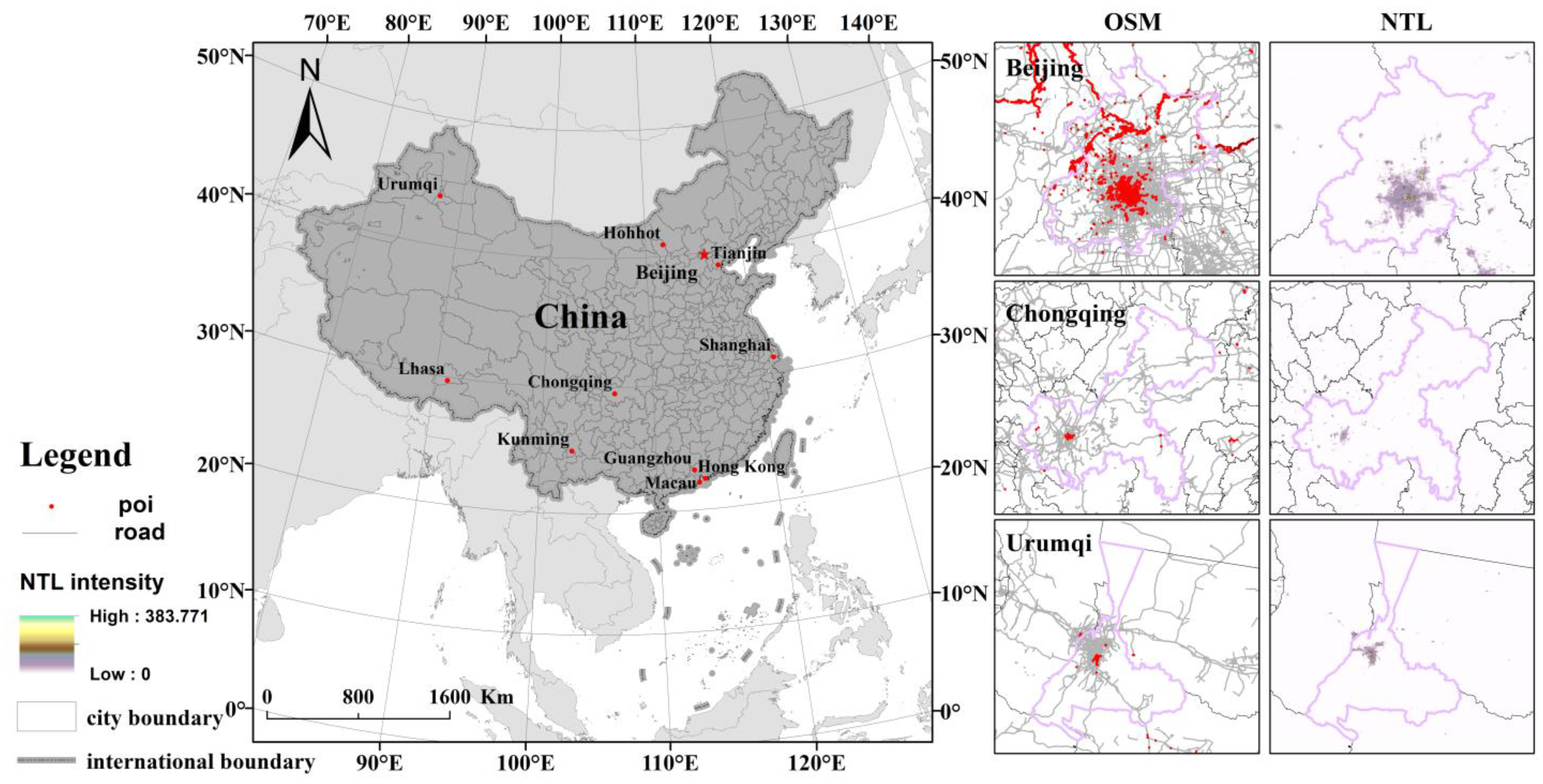
2.1. Study Area
2.2. Data
2.3. Methods
2.3.1. Spatial Autocorrelation
- (1)
- Global spatial autocorrelation
- (2)
- Local spatial autocorrelation
2.3.2. Geographically and Temporally Weighted Regression Model
2.3.3. Residual Analysis
2.3.4. Regression Model Parameters and Description
3. Results
3.1. Analysis of OSM Features and Modeling Capability
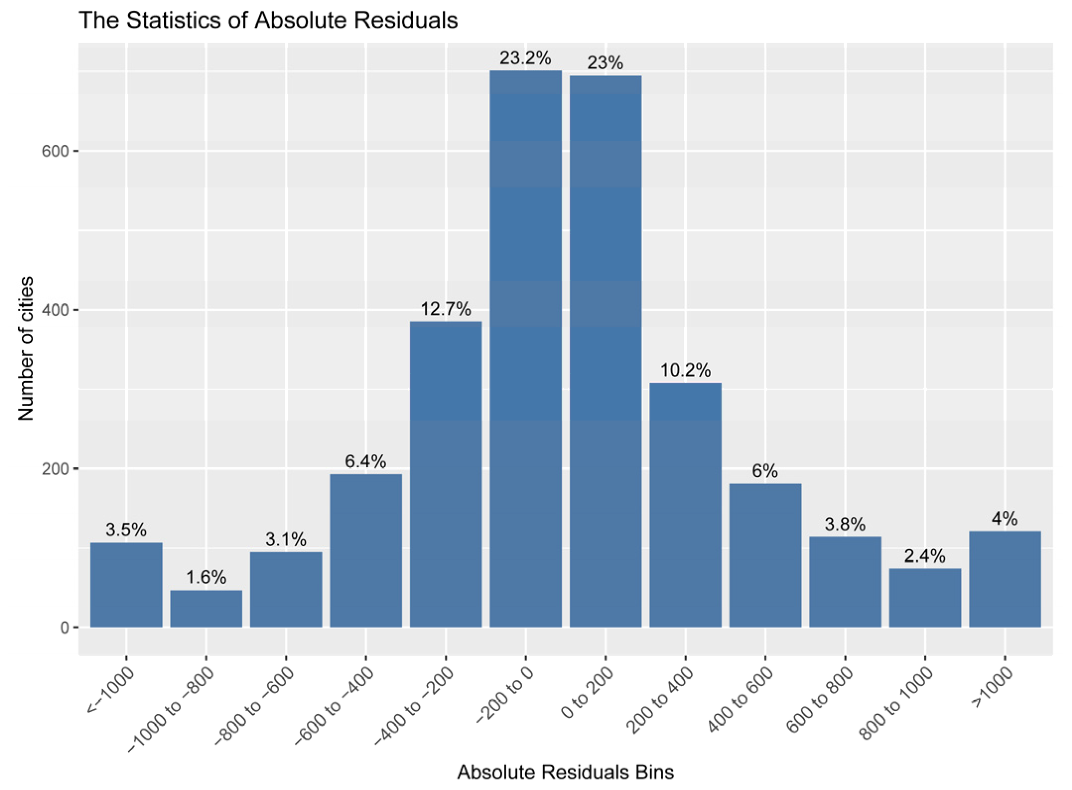
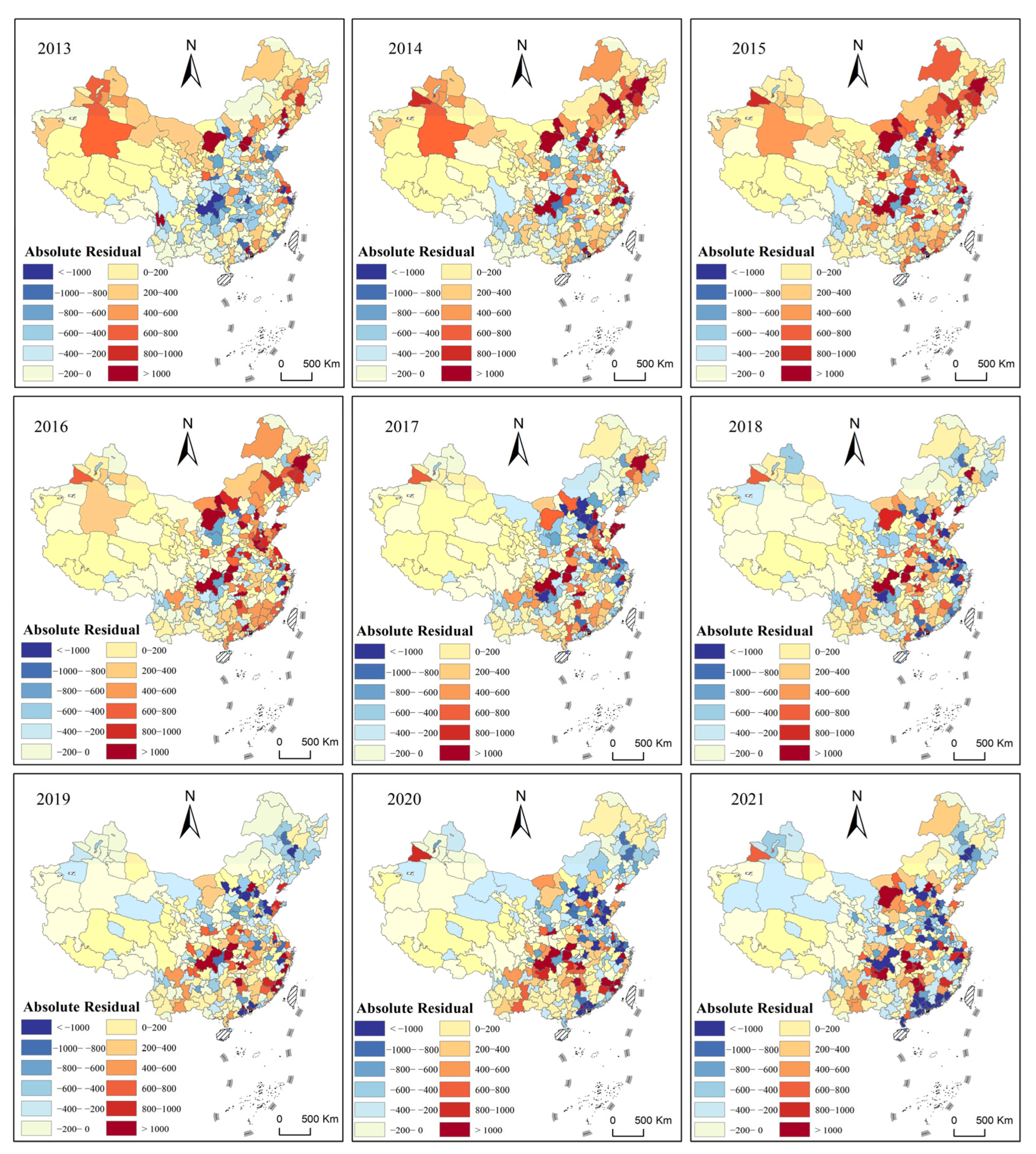
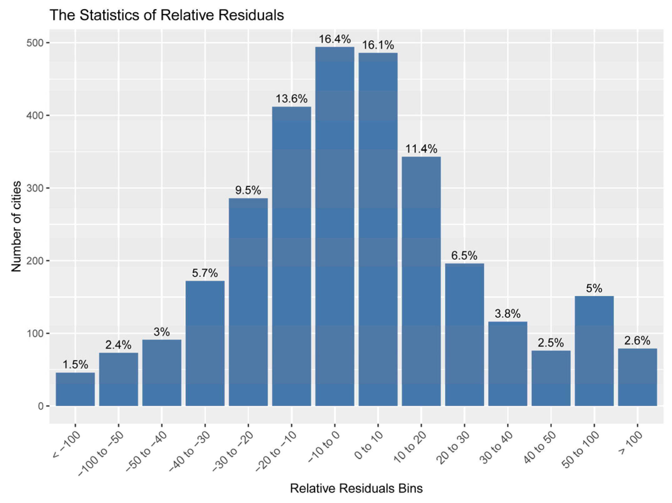
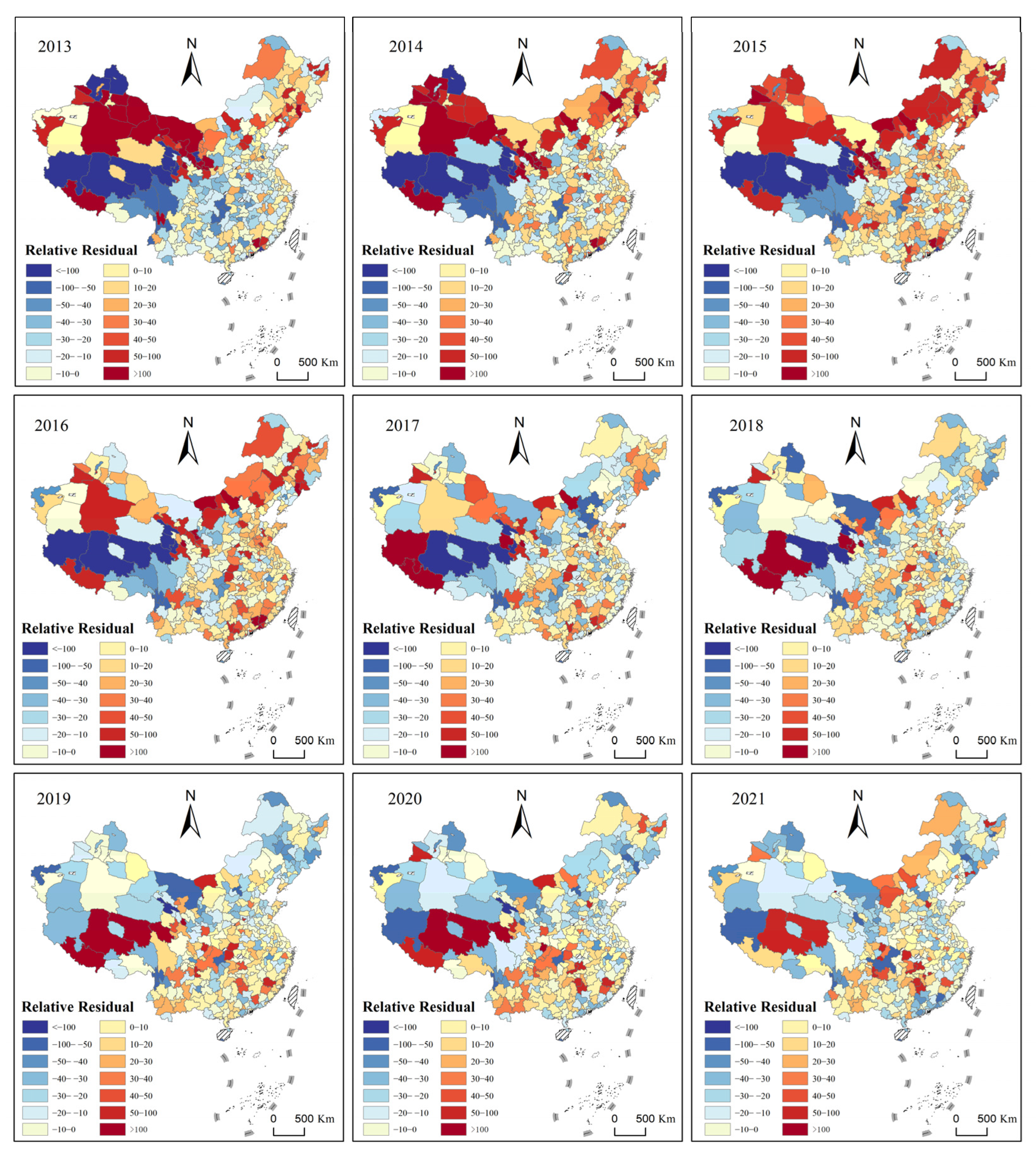
3.1.1. Residual Analysis
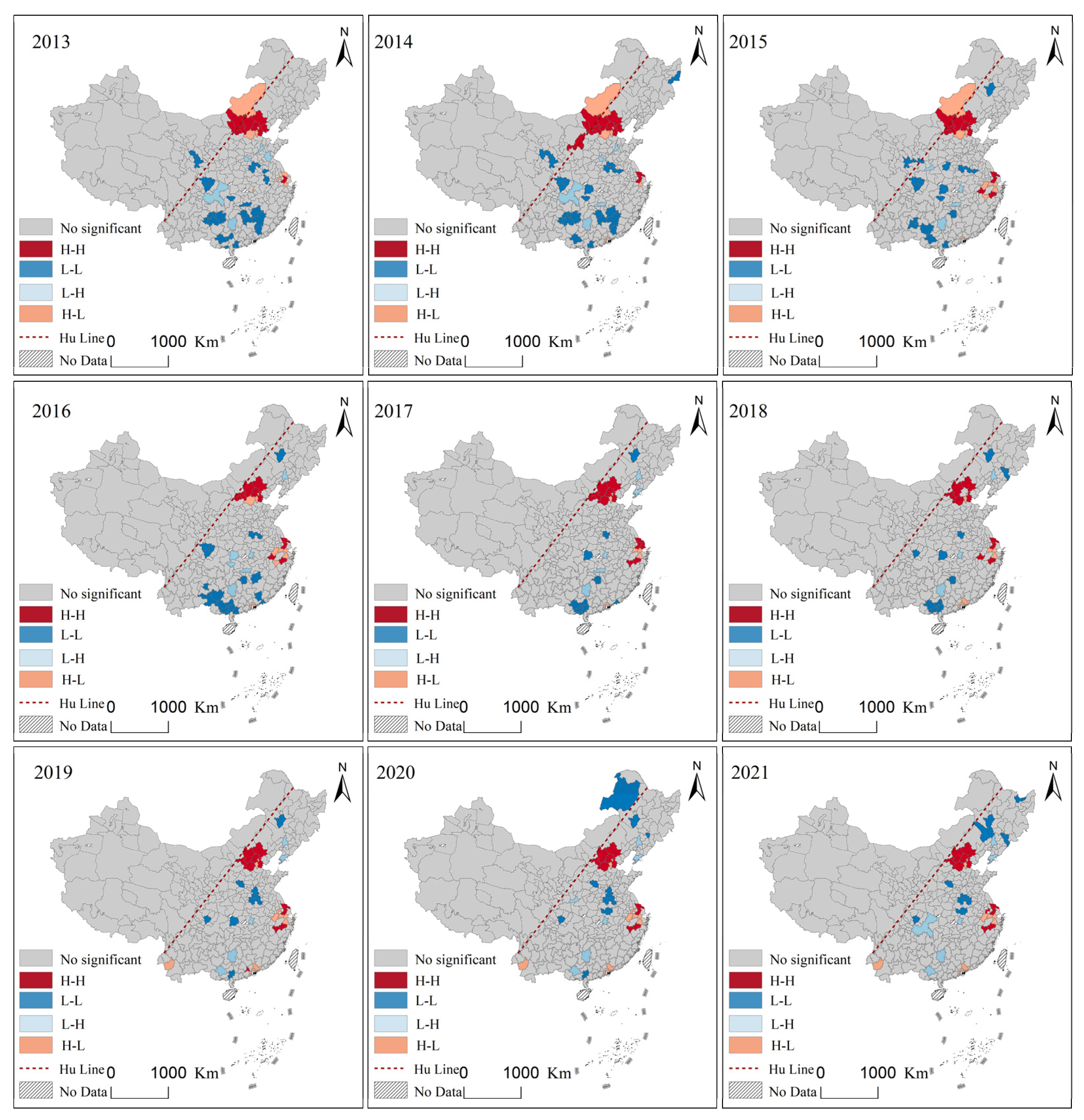
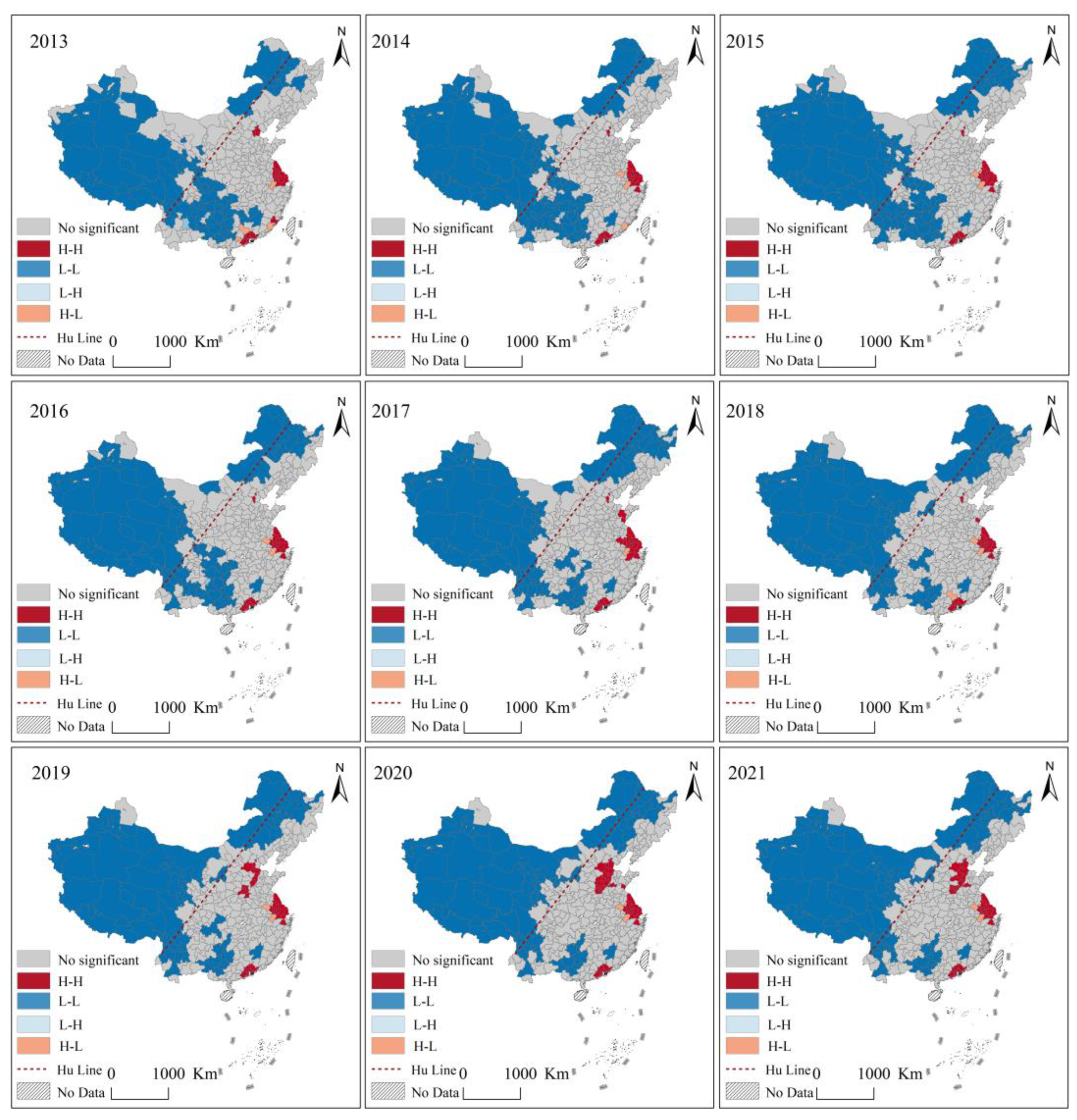
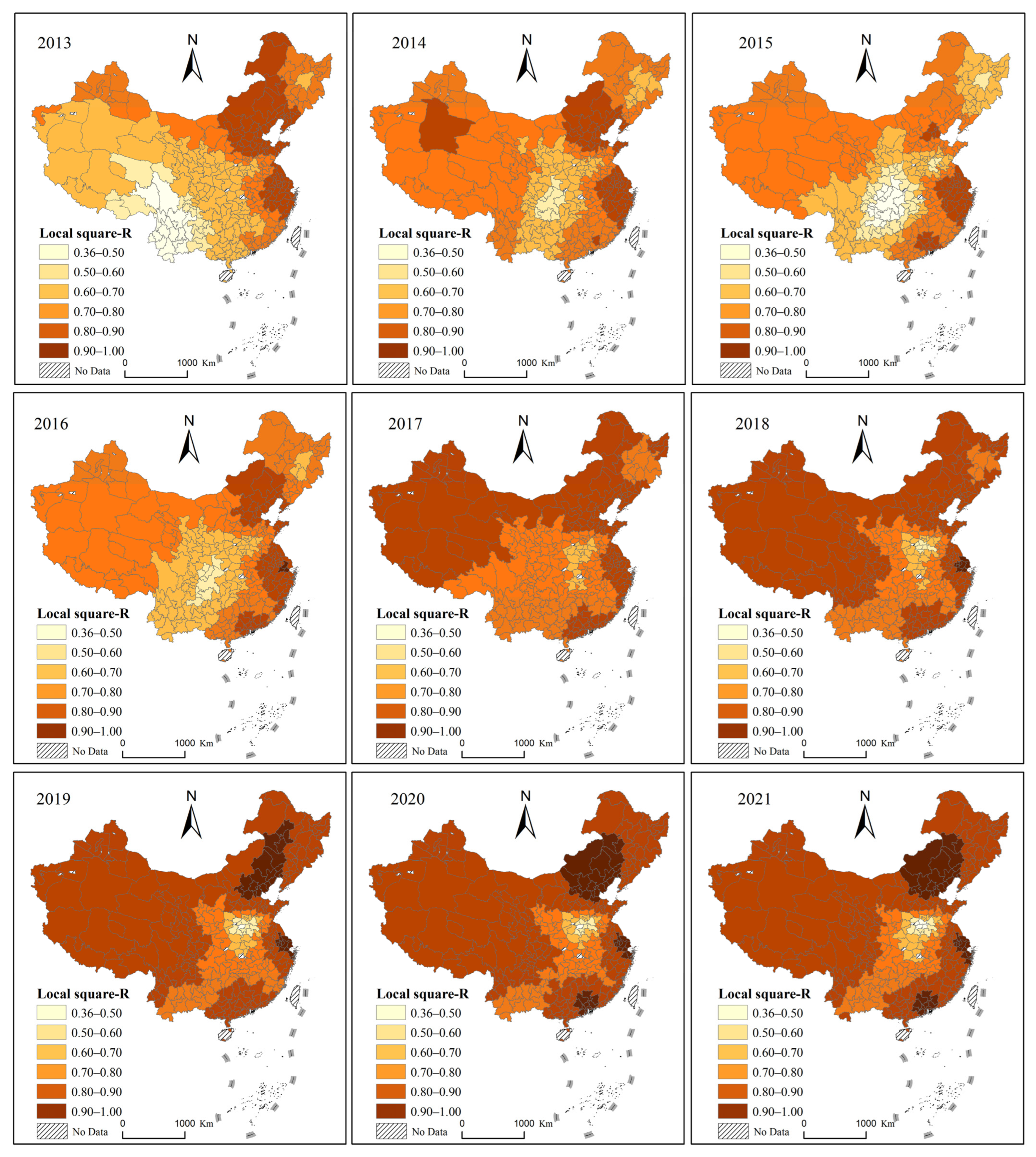
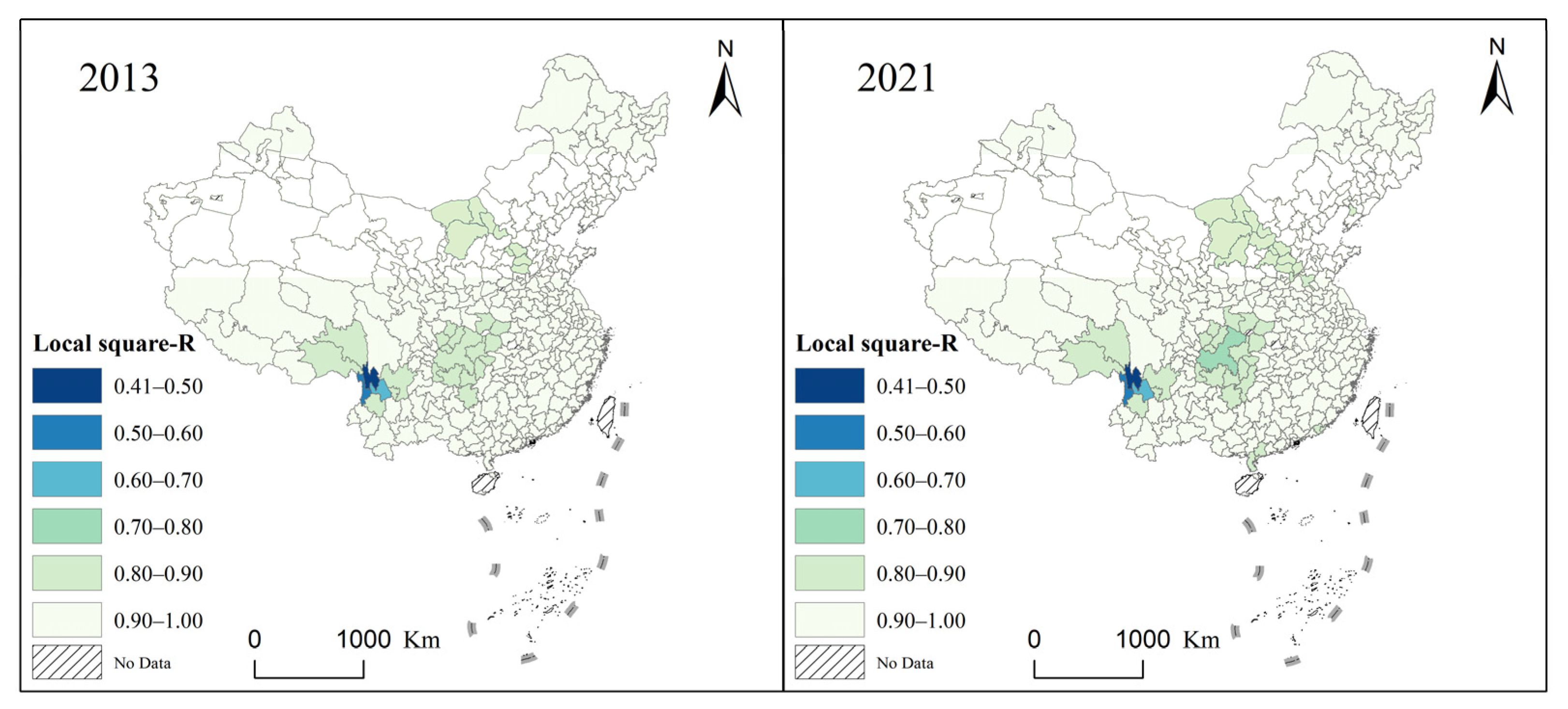
3.1.2. Local Spatial Autocorrelation Features
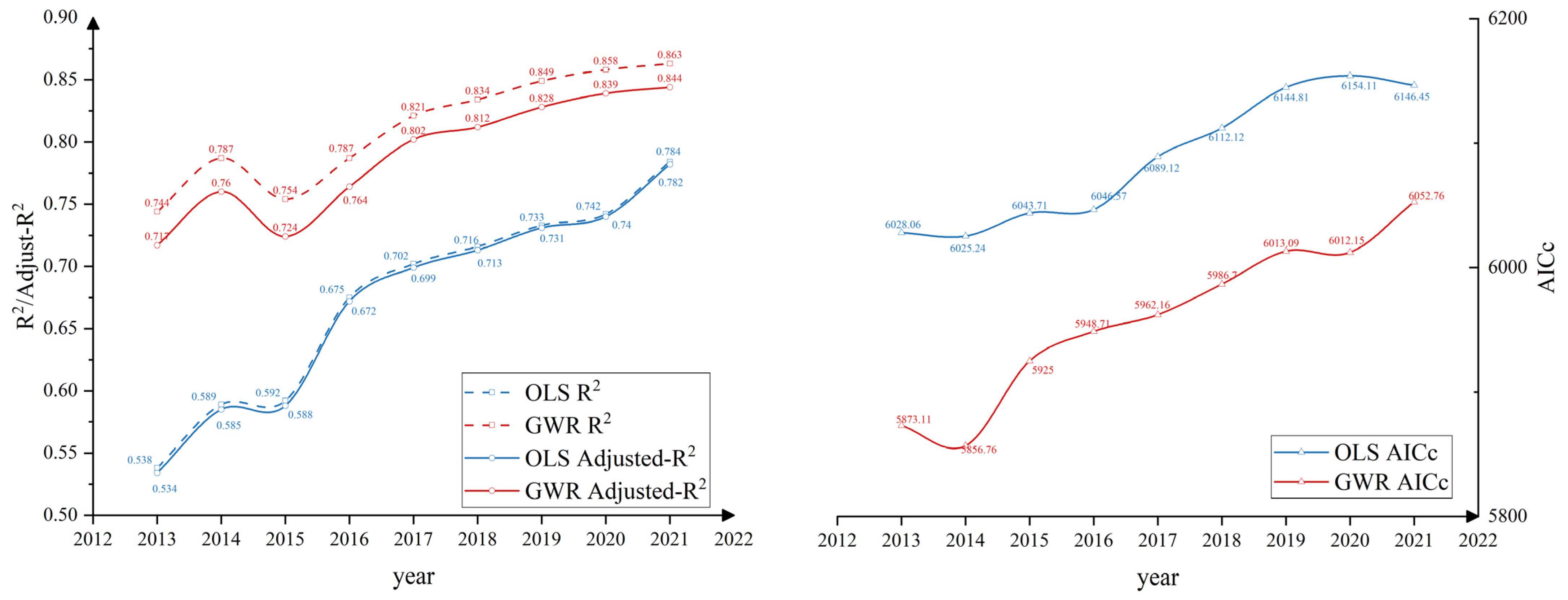
3.1.3. Analysis of OSM Economic Modeling Capability
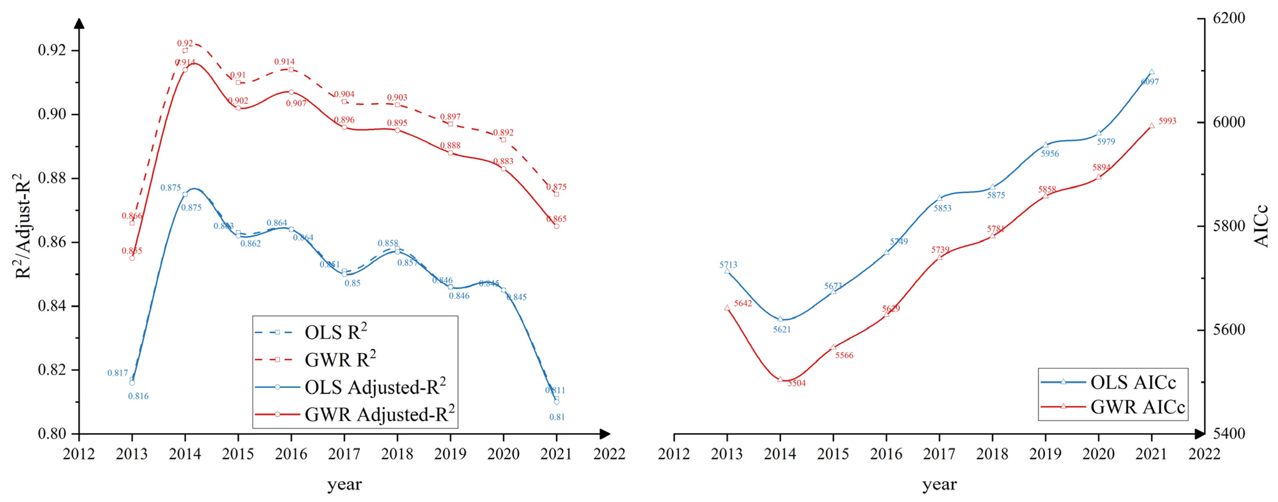
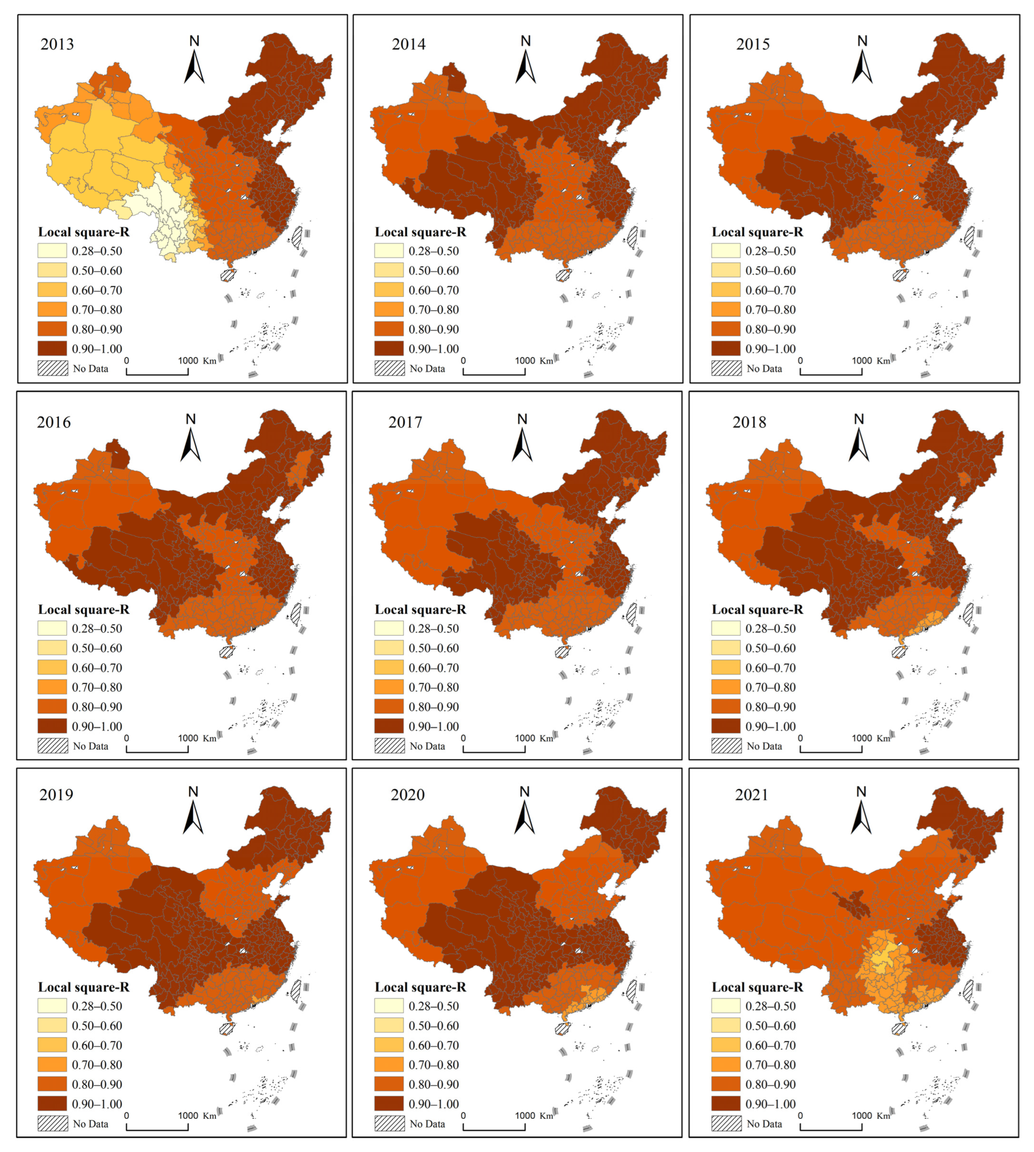
3.2. Analysis of NTL Economic Modeling Capability
3.3. Joint Modeling Results of OSM and NTL
4. Discussion
4.1. Economic Modeling Capabilities of OSM
4.2. Multi-Source Data Evaluation of Economy
4.3. Limitations and Prospects
5. Conclusions
- (1)
- The GTWR model was used to evaluate economic development with OSM data as the single data source from 2013 to 2021, resulting in an R2 of 0.898 and an adjusted R2 of 0.889. When NTL was used as the single data source for economic development evaluation, the R2 was 0.915, and the adjusted R2 was 0.911. OSM data can be considered as a metric to assess economic development, and its evaluation effectiveness is steadily increasing over the years. On the other hand, the evaluation effectiveness of NTL data, as a conventional spatial metric for economic development, is declining. OSM data demonstrate strong correlation with regional socio-economic factors and offer significant advantages over commercial and official maps for economic development evaluation.
- (2)
- The integration and fusion of multiple spatial datasets can serve as a measurement data source for evaluating the spatiotemporal development characteristics of regional economies. The evaluation of economic development using multiple spatial data sources is more reliable than relying on a single data source. VGI data like OSM and spatial metrics like NTL offer empirical and applied research examples for evaluating regional economic development in China. They provide support for broader research and applications in this field.
- (3)
- The GTWR model takes into account spatial and temporal heterogeneity, allowing the establishment of separate regression models at different spatial and temporal points. This enables a more accurate capture of spatiotemporal variations in regional economic characteristics. Compared to conventional global regression analysis, GTWR offers better accuracy and explanatory power in spatiotemporal evaluation of regional economies, resulting in more accurate and reliable assessments of economic development.
Author Contributions
Funding
Data Availability Statement
Conflicts of Interest
References
- United Nations The Sustainable Development Agenda—United Nations Sustainable Development. Available online: https://www.un.org/sustainabledevelopment/development-agenda/ (accessed on 8 September 2023).
- Henderson, J.V.; Storeygard, A.; Weil, D.N. Measuring Economic Growth from Outer Space. Am. Econ. Rev. 2012, 102, 994–1028. [Google Scholar] [CrossRef] [PubMed]
- Chen, X.; Nordhaus, W.D. VIIRS Nighttime Lights in the Estimation of Cross-Sectional and Time-Series GDP. Remote Sens. 2019, 11, 1057. [Google Scholar] [CrossRef]
- Gu, H.; Chen, C.; Lu, Y.; Chu, Y.; Ma, Y. Construction of Regional Economic Development Model Based on Remote Sensing Data. IOP Conf. Ser. Earth Environ. Sci. 2019, 310, 052060. [Google Scholar] [CrossRef]
- Bartik, T. Evaluating the Impacts of Local Economic Development Policies on Local Economic Outcomes: What Has Been Done and What Is Doable? W.E. Upjohn Institute for Employment Research: Kalamazoo, MI, USA, 2002. [Google Scholar]
- Li, B.; Lu, S. Labor Education, Cash Transfers and Student Development: Evidence from China. Int. Rev. Financ. Anal. 2023, 87, 102565. [Google Scholar] [CrossRef]
- Rising, J.A.; Taylor, C.; Ives, M.C.; Ward, R.E.T. Challenges and Innovations in the Economic Evaluation of the Risks of Climate Change. Ecol. Econ. 2022, 197, 107437. [Google Scholar] [CrossRef]
- Wan, G.; Hu, X.; Liu, W. China’s Poverty Reduction Miracle and Relative Poverty: Focusing on the Roles of Growth and Inequality. China Econ. Rev. 2021, 68, 101643. [Google Scholar] [CrossRef]
- Wang, J.; Wei, X.; Guo, Q. A Three-Dimensional Evaluation Model for Regional Carrying Capacity of Ecological Environment to Social Economic Development: Model Development and a Case Study in China. Ecol. Indic. 2018, 89, 348–355. [Google Scholar] [CrossRef]
- Yang, Y.; Liu, Y. The Code of Targeted Poverty Alleviation in China: A Geography Perspective. Geogr. Sustain. 2021, 2, 243–253. [Google Scholar] [CrossRef]
- Jiang, L.; Kuijsten, A. Regional disparities of urbanization levels in China. Chin. J. Popul. Sci. 2001, 1, 45–51. (In Chinese) [Google Scholar]
- Chen, Q.; Ye, T.; Zhao, N.; Ding, M.; Ouyang, Z.; Jia, P.; Yue, W.; Yang, X. Mapping China’s Regional Economic Activity by Integrating Points-of-Interest and Remote Sensing Data with Random Forest. Environ. Plan. B Urban Anal. City Sci. 2021, 48, 1876–1894. [Google Scholar] [CrossRef]
- Ivković, A. Limitations of the GDP as a measure of progress and well-being. Ekonomski Vjesnik 2016, 29, 257–272. [Google Scholar]
- Kinyondo, A.; Pelizzo, R. Poor Quality of Data in Africa: What Are the Issues? Politics Policy 2018, 46, 851–877. [Google Scholar] [CrossRef]
- Brock, G. A Remote Sensing Look at the Economy of a Russian Region (Rostov) Adjacent to the Ukrainian Crisis. J. Policy Model. 2019, 41, 416–431. [Google Scholar] [CrossRef]
- Chen, D.; Zhang, Y.; Yao, Y.; Hong, Y.; Guan, Q.; Tu, W. Exploring the Spatial Differentiation of Urbanization on Two Sides of the Hu Huanyong Line—Based on Nighttime Light Data and Cellular Automata. Appl. Geogr. 2019, 112, 102081. [Google Scholar] [CrossRef]
- Lin, J.; Luo, S.; Huang, Y. Poverty Estimation at the County Level by Combining LuoJia1-01 Nighttime Light Data and Points of Interest. Geocarto Int. 2022, 37, 3590–3606. [Google Scholar] [CrossRef]
- Shao, Z.; Li, X. Multi-Scale Estimation of Poverty Rate Using Night-Time Light Imagery. Int. J. Appl. Earth Obs. Geoinf. 2023, 121, 103375. [Google Scholar] [CrossRef]
- Wan, N.; Du, Y.; Liang, F.; Yi, J.; Qian, J.; Tu, W.; Huang, S. Nighttime Light Satellite Images Reveal Uneven Socioeconomic Development along China’s Land Border. Appl. Geogr. 2023, 152, 102899. [Google Scholar] [CrossRef]
- Zhao, N.; Cao, G.; Zhang, W.; Samson, E.L. Tweets or Nighttime Lights: Comparison for Preeminence in Estimating Socioeconomic Factors. ISPRS J. Photogramm. Remote Sens. 2018, 146, 1–10. [Google Scholar] [CrossRef]
- Cao, C.; Zhang, B.; Xia, F.; Bai, Y. Exploring VIIRS Night Light Long-Term Time Series with CNN/SI for Urban Change Detection and Aerosol Monitoring. Remote Sens. 2022, 14, 3126. [Google Scholar] [CrossRef]
- Chen, T.-H.K.; Prishchepov, A.V.; Fensholt, R.; Sabel, C.E. Detecting and Monitoring Long-Term Landslides in Urbanized Areas with Nighttime Light Data and Multi-Seasonal Landsat Imagery across Taiwan from 1998 to 2017. Remote Sens. Environ. 2019, 225, 317–327. [Google Scholar] [CrossRef]
- Gibson, J.; Olivia, S.; Boe-Gibson, G.; Li, C. Which Night Lights Data Should We Use in Economics, and Where? J. Dev. Econ. 2021, 149, 102602. [Google Scholar] [CrossRef]
- Li, G.; Fan, J.; Zhou, Y.; Zhang, Y. Development Characteristics Estimation of Shandong Peninsula Urban Agglomeration Using VIIRS Night Light Data. Remote Sens. Technol. Appl. 2021, 35, 1348–1359. [Google Scholar]
- Li, X.; Xu, H.; Chen, X.; Li, C. Potential of NPP-VIIRS Nighttime Light Imagery for Modeling the Regional Economy of China. Remote Sens. 2013, 5, 3057–3081. [Google Scholar] [CrossRef]
- Puri, P.; Puri, V. Observing Economics through Geography: COVID-19 and Night-Light Data Analysis of Bangladesh and Sri Lanka (2017–2021). ACADEMICIA Int. Multidiscip. Res. J. 2022, 12, 42–54. [Google Scholar] [CrossRef]
- Tan, M.; Li, X.; Li, S.; Xin, L.; Wang, X.; Li, Q.; Li, W.; Li, Y.; Xiang, W. Modeling Population Density Based on Nighttime Light Images and Land Use Data in China. Appl. Geogr. 2018, 90, 239–247. [Google Scholar] [CrossRef]
- Sutton, P.C.; Costanza, R. Global Estimates of Market and Non-Market Values Derived from Nighttime Satellite Imagery, Land Cover, and Ecosystem Service Valuation. Ecol. Econ. 2002, 41, 509–527. [Google Scholar] [CrossRef]
- Wang, X.; Rafa, M.; Moyer, J.D.; Li, J.; Scheer, J.; Sutton, P. Estimation and Mapping of Sub-National GDP in Uganda Using NPP-VIIRS Imagery. Remote Sens. 2019, 11, 163. [Google Scholar] [CrossRef]
- Li, D.; Li, X. An Overview on Data Mining of Nighttime Light Remote Sensing. Acta Geod. Et Cartogr. Sin. 2015, 44, 591–601. [Google Scholar] [CrossRef]
- Li, C.; Huo, Z.; Wang, X.; Wu, Y. Study on Spatio-Temporal Modelling between NPP-VIIRS Night-Time Light Intensity and GDP for Major Urban Agglomerations in China. Int. J. Remote Sens. 2022, 1–24. [Google Scholar] [CrossRef]
- Chen, Z.; Yu, B.; Yang, C.; Zhou, Y.; Yao, S.; Qian, X.; Wang, C.; Wu, B.; Wu, J. An Extended Time Series (2000–2018) of Global NPP-VIIRS-like Nighttime Light Data from a Cross-Sensor Calibration. Earth Syst. Sci. Data 2021, 13, 889–906. [Google Scholar] [CrossRef]
- Liang, H.; Guo, Z.; Wu, J.; Chen, Z. GDP Spatialization in Ningbo City Based on NPP/VIIRS Night-Time Light and Auxiliary Data Using Random Forest Regression. Adv. Space Res. 2020, 65, 481–493. [Google Scholar] [CrossRef]
- Shi, K.; Yu, B.; Huang, Y.; Hu, Y.; Yin, B.; Chen, Z.; Chen, L.; Wu, J. Evaluating the Ability of NPP-VIIRS Nighttime Light Data to Estimate the Gross Domestic Product and the Electric Power Consumption of China at Multiple Scales: A Comparison with DMSP-OLS Data. Remote Sens. 2014, 6, 1705–1724. [Google Scholar] [CrossRef]
- Li, X.; Ma, R.; Zhang, Q.; Li, D.; Liu, S.; He, T.; Zhao, L. Anisotropic Characteristic of Artificial Light at Night–Systematic Investigation with VIIRS DNB Multi-Temporal Observations. Remote Sens. Environ. 2019, 233, 111357. [Google Scholar] [CrossRef]
- Goodchild, M.F. Citizens as Sensors: The World of Volunteered Geography. GeoJournal 2007, 69, 211–221. [Google Scholar] [CrossRef]
- See, L.; Mooney, P.; Foody, G.; Bastin, L.; Comber, A.; Estima, J.; Fritz, S.; Kerle, N.; Jiang, B.; Laakso, M.; et al. Crowdsourcing, Citizen Science or Volunteered Geographic Information? The Current State of Crowdsourced Geographic Information. ISPRS Int. J. Geo-Inf. 2016, 5, 55. [Google Scholar] [CrossRef]
- Goodchild, M.F.; Li, L. Assuring the Quality of Volunteered Geographic Information. Spat. Stat. 2012, 1, 110–120. [Google Scholar] [CrossRef]
- Feige, E.L.; Urban, I. Measuring Underground (Unobserved, Non-Observed, Unrecorded) Economies in Transition Countries: Can We Trust GDP? J. Comp. Econ. 2008, 36, 287–306. [Google Scholar] [CrossRef]
- Jokar Arsanjani, J.; Mooney, P.; Zipf, A.; Schauss, A. Quality Assessment of the Contributed Land Use Information from OpenStreetMap Versus Authoritative Datasets. In OpenStreetMap in GIScience: Experiences, Research, and Applications; Jokar Arsanjani, J., Zipf, A., Mooney, P., Helbich, M., Eds.; Lecture Notes in Geoinformation and Cartography; Springer International Publishing: Cham, Switzerland, 2015; pp. 37–58. ISBN 978-3-319-14280-7. [Google Scholar]
- Neis, P.; Zielstra, D. Recent Developments and Future Trends in Volunteered Geographic Information Research: The Case of OpenStreetMap. Future Internet 2014, 6, 76–106. [Google Scholar] [CrossRef]
- Zheng, S.; Zheng, J. Assessing the Completeness and Positional Accuracy of OpenStreetMap in China. In Thematic Cartography for the Society; Bandrova, T., Konecny, M., Zlatanova, S., Eds.; Lecture Notes in Geoinformation and Cartography; Springer International Publishing: Cham, Switzerland, 2014; pp. 171–189. ISBN 978-3-319-08180-9. [Google Scholar]
- Moradi, M.; Roche, S.; Mostafavi, M.A. Exploring Five Indicators for the Quality of OpenStreetMap Road Networks: A Case Study of Québec, Canada. Geomatica 2022, 75, 178–208. [Google Scholar] [CrossRef]
- Barrington-Leigh, C.; Millard-Ball, A. Global Trends toward Urban Street-Network Sprawl. Proc. Natl. Acad. Sci. USA 2020, 117, 1941–1950. [Google Scholar] [CrossRef]
- Hadimlioglu, I.A.; King, S.A. City Maker: Reconstruction of Cities from OpenStreetMap Data for Environmental Visualization and Simulations. ISPRS Int. J. Geo-Inf. 2019, 8, 298. [Google Scholar] [CrossRef]
- Zhang, L.; Pfoser, D. Using OpenStreetMap Point-of-Interest Data to Model Urban Change—A Feasibility Study. PLoS ONE 2019, 14, e0212606. [Google Scholar] [CrossRef] [PubMed]
- Herfort, B.; Lautenbach, S.; Porto de Albuquerque, J.; Anderson, J.; Zipf, A. The Evolution of Humanitarian Mapping within the OpenStreetMap Community. Sci. Rep. 2021, 11, 3037. [Google Scholar] [CrossRef] [PubMed]
- Liu, B.; Shi, Y.; Li, D.-J.; Wang, Y.-D.; Fernandez, G.; Tsou, M.-H. An Economic Development Evaluation Based on the OpenStreetMap Road Network Density: The Case Study of 85 Cities in China. ISPRS Int. J. Geo-Inf. 2020, 9, 517. [Google Scholar] [CrossRef]
- Borkowska, S.; Pokonieczny, K. Analysis of OpenStreetMap Data Quality for Selected Counties in Poland in Terms of Sustainable Development. Sustainability 2022, 14, 3728. [Google Scholar] [CrossRef]
- Budhathoki, N.R. Participants’ Motivations to Contribute Geographic Information in an Online Community; University of Illinois at Urbana-Champaign: Champaign, IL, USA, 2010; ISBN 1-124-58124-3. [Google Scholar]
- Cheng, F.; Liu, S.; Hou, X.; Zhang, Y.; Dong, S.; Coxixo, A.; Liu, G. Urban Land Extraction Using DMSP/OLS Nighttime Light Data and OpenStreetMap Datasets for Cities in China at Different Development Levels. IEEE J. Sel. Top. Appl. Earth Obs. Remote Sens. 2018, 11, 2587–2599. [Google Scholar] [CrossRef]
- Shi, L.; Ling, F. Local Climate Zone Mapping Using Multi-Source Free Available Datasets on Google Earth Engine Platform. Land 2021, 10, 454. [Google Scholar] [CrossRef]
- Wang, L.; Fan, H.; Wang, Y. An Estimation of Housing Vacancy Rate Using NPP-VIIRS Night-Time Light Data and OpenStreetMap Data. Int. J. Remote Sens. 2019, 40, 8566–8588. [Google Scholar] [CrossRef]
- Ma, D.; Guo, R.; Jing, Y.; Zheng, Y.; Zhao, Z.; Yang, J. Intra-Urban Scaling Properties Examined by Automatically Extracted City Hotspots from Street Data and Nighttime Light Imagery. Remote Sens. 2021, 13, 1322. [Google Scholar] [CrossRef]
- Griffith, D.A.; Arbia, G. Detecting Negative Spatial Autocorrelation in Georeferenced Random Variables. Int. J. Geogr. Inf. Sci. 2010, 24, 417–437. [Google Scholar] [CrossRef]
- Anselin, L.; Syabri, I.; Kho, Y. GeoDa: An Introduction to Spatial Data Analysis. In Handbook of Applied Spatial Analysis: Software Tools, Methods and Applications; Fischer, M.M., Getis, A., Eds.; Springer: Berlin/Heidelberg, Germany, 2010; pp. 73–89. ISBN 978-3-642-03647-7. [Google Scholar]
- Wu, Y.; Zhu, X.; Gao, W.; Qian, F. The Spatial Characteristics of Coupling Relationship between Urbanization and Eco-Environment in the Pan Yangtze River Delta. Energy Procedia 2018, 152, 1121–1126. [Google Scholar] [CrossRef]
- Li, C.; Wu, K.; Gao, X. Manufacturing Industry Agglomeration and Spatial Clustering: Evidence from Hebei Province, China. Environ. Dev. Sustain. 2020, 22, 2941–2965. [Google Scholar] [CrossRef]
- Moran, P.A.P. Notes on Continuous Stochastic Phenomena. Biometrika 1950, 37, 17–23. [Google Scholar] [CrossRef] [PubMed]
- Anselin, L. Local Indicators of Spatial Association—LISA. Geogr. Anal. 1995, 27, 93–115. [Google Scholar] [CrossRef]
- Ord, J.K.; Getis, A. Local Spatial Autocorrelation Statistics: Distributional Issues and an Application. Geogr. Anal. 1995, 27, 286–306. [Google Scholar] [CrossRef]
- Qiu, M.; Zuo, Q.; Wu, Q.; Yang, Z.; Zhang, J. Water Ecological Security Assessment and Spatial Autocorrelation Analysis of Prefectural Regions Involved in the Yellow River Basin. Sci. Rep. 2022, 12, 5105. [Google Scholar] [CrossRef] [PubMed]
- Huang, B.; Wu, B.; Barry, M. Geographically and Temporally Weighted Regression for Modeling Spatio-Temporal Variation in House Prices. Int. J. Geogr. Inf. Sci. 2010, 24, 383–401. [Google Scholar] [CrossRef]
- Yu, D. Understanding Regional Development Mechanisms in Greater Beijing Area, China, 1995–2001, from a Spatial–Temporal Perspective. GeoJournal 2014, 79, 195–207. [Google Scholar] [CrossRef]
- Yu, D.; Lv, B. Challenging the Current Measurement of China’s Provincial Total Factor Productivity: A Spatial Econometric Perspective. China Soft Sci. 2009, 11, 160–170. [Google Scholar]
- Li, W.; Ji, Z.; Dong, F. Spatio-Temporal Evolution Relationships between Provincial CO2 Emissions and Driving Factors Using Geographically and Temporally Weighted Regression Model. Sustain. Cities Soc. 2022, 81, 103836. [Google Scholar] [CrossRef]
- Akaike, H. Information Theory and an Extension of the Maximum Likelihood Principle. In Selected Papers of Hirotugu Akaike; Parzen, E., Tanabe, K., Kitagawa, G., Eds.; Springer Series in Statistics; Springer: New York, NY, USA, 1998; pp. 199–213. ISBN 978-1-4612-1694-0. [Google Scholar]
- Hu, H.Y. The Distribution of Population in China, with Statistics and Maps. Acta Geogr. Sin. 1935, 2, 33–74. [Google Scholar] [CrossRef]
- Gao, J.; Li, S. Detecting Spatially Non-Stationary and Scale-Dependent Relationships between Urban Landscape Fragmentation and Related Factors Using Geographically Weighted Regression. Appl. Geogr. 2011, 31, 292–302. [Google Scholar] [CrossRef]
- Boscolo, D.; Paul Metzger, J. Isolation Determines Patterns of Species Presence in Highly Fragmented Landscapes. Ecography 2011, 34, 1018–1029. [Google Scholar] [CrossRef]
- Gao, Y.; Huang, J.; Li, S.; Li, S. Spatial Pattern of Non-Stationarity and Scale-Dependent Relationships between NDVI and Climatic Factors—A Case Study in Qinghai-Tibet Plateau, China. Ecol. Indic. 2012, 20, 170–176. [Google Scholar] [CrossRef]
- Auxier, B.; Anderson, M. Social Media Use in 2021; Pew Research Center: Washington, DC, USA, 2021; Volume 1, pp. 1–4. [Google Scholar]
- Bimber, B. Measuring the Gender Gap on the Internet. Soc. Sci. Q. 2000, 81, 868–876. [Google Scholar]
- Calvert, S.L.; Rideout, V.J.; Woolard, J.L.; Barr, R.F.; Strouse, G.A. Age, Ethnicity, and Socioeconomic Patterns in Early Computer Use: A National Survey. Am. Behav. Sci. 2005, 48, 590–607. [Google Scholar] [CrossRef]
- Song, Y.; Li, X.; Tao, G.; Liu, J. Exploring the Characteristics and Drivers of Expansion in the Shandong Peninsula Urban Agglomeration Based on Nighttime Light Data. IEEE J. Sel. Top. Appl. Earth Obs. Remote Sens. 2023, 16, 8535–8549. [Google Scholar] [CrossRef]
- Xu, G.; Su, J.; Xia, C.; Li, X.; Xiao, R. Spatial Mismatches between Nighttime Light Intensity and Building Morphology in Shanghai, China. Sustain. Cities Soc. 2022, 81, 103851. [Google Scholar] [CrossRef]
- Yang, Z.; Chen, Y.; Guo, G.; Zheng, Z.; Wu, Z. Using Nighttime Light Data to Identify the Structure of Polycentric Cities and Evaluate Urban Centers. Sci. Total Environ. 2021, 780, 146586. [Google Scholar] [CrossRef]
- Li, S.; Zhang, T.; Yang, Z.; Li, X.; Xu, H. Night time light satellite data for evaluating the socioeconomics in central Asia. Int. Arch. Photogramm. Remote Sens. Spatial Inf. Sci. 2017, 42, 1237–1243. [Google Scholar] [CrossRef]
- Huang, Z.; Li, S.; Gao, F.; Wang, F.; Lin, J.; Tan, Z. Evaluating the Performance of LBSM Data to Estimate the Gross Domestic Product of China at Multiple Scales: A Comparison with NPP-VIIRS Nighttime Light Data. J. Clean. Prod. 2021, 328, 129558. [Google Scholar] [CrossRef]
- Cui, Y.; Shi, K.; Jiang, L.; Qiu, L.; Wu, S. Identifying and Evaluating the Nighttime Economy in China Using Multisource Data. IEEE Geosci. Remote Sens. Lett. 2021, 18, 1906–1910. [Google Scholar] [CrossRef]
- Wong, D.W.S. The Modifiable Areal Unit Problem (MAUP). In WorldMinds: Geographical Perspectives on 100 Problems: Commemorating the 100th Anniversary of the Association of American Geographers 1904–2004; Janelle, D.G., Warf, B., Hansen, K., Eds.; Springer: Dordrecht, The Netherlands, 2004; pp. 571–575. ISBN 978-1-4020-2352-1. [Google Scholar]
- Encalada-Abarca, L.; Ferreira, C.C.; Rocha, J. Measuring Tourism Intensification in Urban Destinations: An Approach Based on Fractal Analysis. J. Travel Res. 2022, 61, 394–413. [Google Scholar] [CrossRef]
- Long, Y.; Zhai, W.; Shen, Y.; Ye, X. Understanding Uneven Urban Expansion with Natural Cities Using Open Data. Landsc. Urban Plan. 2018, 177, 281–293. [Google Scholar] [CrossRef]


| Data Name | Variable | Description | Unit | Min. | Max. | Standard Deviation |
| OSM | POI Count | POI Total Count | Per | 0.00 | 14162 | 720.91 |
| POI Density | POI Density | Per/km2 | 0.00 | 1.4690 | 0.08776 | |
| Road Density | Road Network Density | km/km2 | 0.0049 | 8.0836 | 0.76310 | |
| NTL | TNL | Total nighttime light | 209.74 | 505,994 | 56,317.75 | |
| Economy | GDP | Gross Domestic Product | 100 million CNY | 7.3471 | 43,214.9 | 3846.57 |
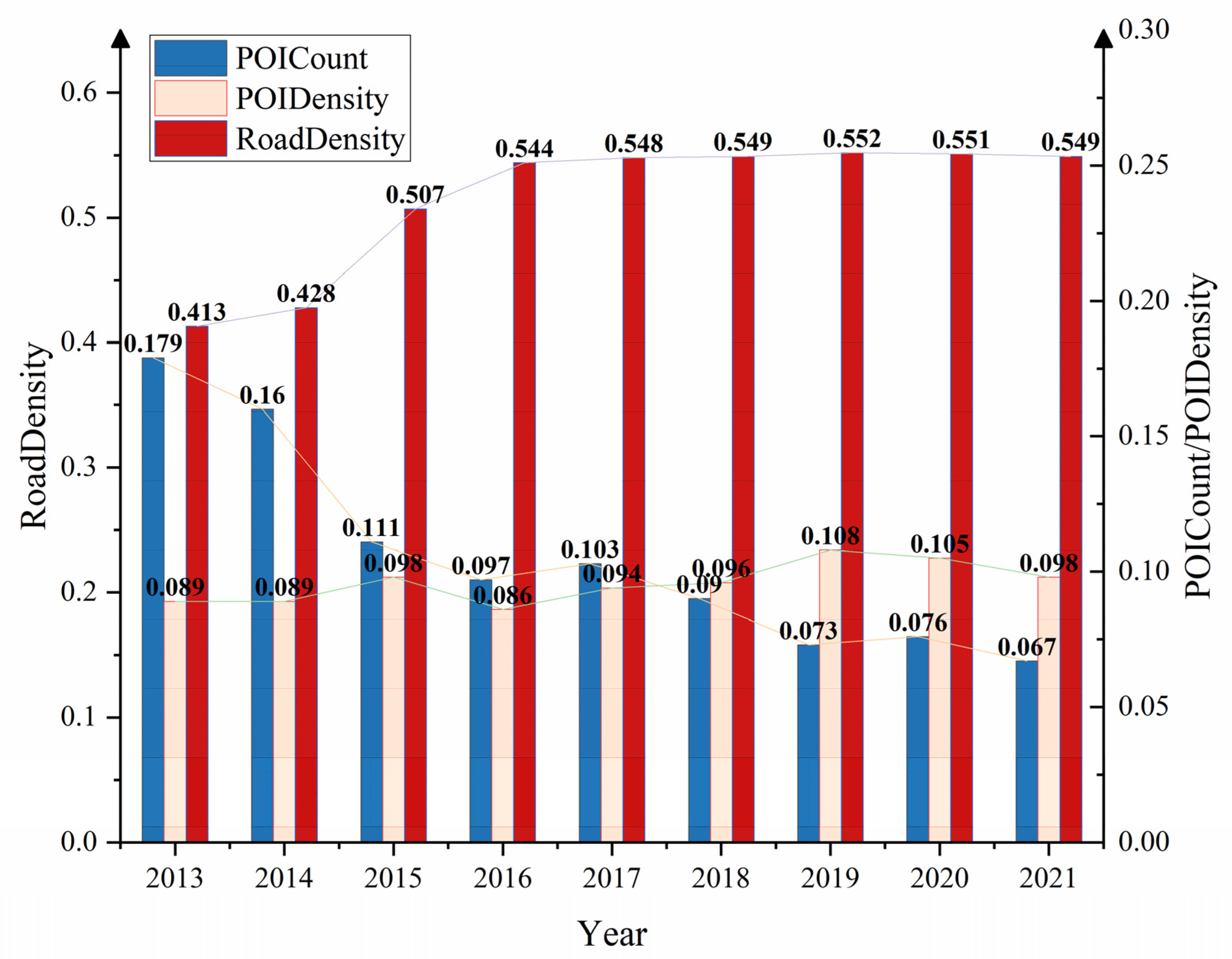
| Data | Year | Moran Index | p-Value | Z-Value |
|---|---|---|---|---|
| POI Count | 2013 | 0.179 | 0.002 | 6.564 |
| 2014 | 0.16 | 0.003 | 5.909 | |
| 2015 | 0.111 | 0.011 | 3.676 | |
| 2016 | 0.097 | 0.014 | 3.562 | |
| 2017 | 0.103 | 0.015 | 3.537 | |
| 2018 | 0.09 | 0.016 | 3.511 | |
| 2019 | 0.073 | 0.029 | 2.46 | |
| 2020 | 0.076 | 0.026 | 2.529 | |
| 2021 | 0.067 | 0.032 | 2.285 | |
| POI Density | 2013 | 0.089 | 0.017 | 2.931 |
| 2014 | 0.089 | 0.013 | 3.091 | |
| 2015 | 0.098 | 0.005 | 3.478 | |
| 2016 | 0.086 | 0.018 | 2.849 | |
| 2017 | 0.094 | 0.017 | 2.969 | |
| 2018 | 0.096 | 0.018 | 3.099 | |
| 2019 | 0.108 | 0.009 | 3.582 | |
| 2020 | 0.105 | 0.011 | 3.405 | |
| 2021 | 0.098 | 0.011 | 3.203 | |
| Road Density | 2013 | 0.413 | 0.001 | 12.549 |
| 2014 | 0.428 | 0.001 | 13.49 | |
| 2015 | 0.507 | 0.001 | 14.785 | |
| 2016 | 0.544 | 0.001 | 16.019 | |
| 2017 | 0.548 | 0.001 | 16.717 | |
| 2018 | 0.549 | 0.001 | 16.28 | |
| 2019 | 0.552 | 0.001 | 16.299 | |
| 2020 | 0.551 | 0.001 | 16.192 | |
| 2021 | 0.549 | 0.001 | 16.034 |
| Model | R2 | Adjusted R2 | AICc | Bandwidth |
|---|---|---|---|---|
| GTWR | 0.898 | 0.889 | 51,992.28 | 16 |
| OLS | 0.675 | 0.674 | 55,066.95 |
| Model | R2 | Adjusted R2 | AICc | Bandwidth |
|---|---|---|---|---|
| GTWR | 0.915 | 0.911 | 51,200.73 | 26 |
| OLS | 0.842 | 0.842 | 52,882.25 |
| Model | R2 | Adjusted R2 | AICc | Bandwidth |
|---|---|---|---|---|
| GTWR | 0.960 | 0.957 | 49,112.71 | 26 |
| OLS | 0.887 | 0.887 | 51,863.65 |
| Local R2 | Number of Cities | Percentage (%) |
|---|---|---|
| 0.4–0.5 | 9 | 0.30 |
| 0.5–0.6 | 9 | 0.30 |
| 0.6–0.7 | 9 | 0.30 |
| 0.7–0.8 | 1 | 0.03 |
| 0.8–0.9 | 273 | 9.04 |
| 0.9–1.0 | 2720 | 90.04 |
Disclaimer/Publisher’s Note: The statements, opinions and data contained in all publications are solely those of the individual author(s) and contributor(s) and not of MDPI and/or the editor(s). MDPI and/or the editor(s) disclaim responsibility for any injury to people or property resulting from any ideas, methods, instructions or products referred to in the content. |
© 2024 by the authors. Licensee MDPI, Basel, Switzerland. This article is an open access article distributed under the terms and conditions of the Creative Commons Attribution (CC BY) license (https://creativecommons.org/licenses/by/4.0/).
Share and Cite
Wang, Z.; Zheng, J.; Han, C.; Lu, B.; Yu, D.; Yang, J.; Han, L. Exploring the Potential of OpenStreetMap Data in Regional Economic Development Evaluation Modeling. Remote Sens. 2024, 16, 239. https://doi.org/10.3390/rs16020239
Wang Z, Zheng J, Han C, Lu B, Yu D, Yang J, Han L. Exploring the Potential of OpenStreetMap Data in Regional Economic Development Evaluation Modeling. Remote Sensing. 2024; 16(2):239. https://doi.org/10.3390/rs16020239
Chicago/Turabian StyleWang, Zhe, Jianghua Zheng, Chuqiao Han, Binbin Lu, Danlin Yu, Juan Yang, and Linzhi Han. 2024. "Exploring the Potential of OpenStreetMap Data in Regional Economic Development Evaluation Modeling" Remote Sensing 16, no. 2: 239. https://doi.org/10.3390/rs16020239
APA StyleWang, Z., Zheng, J., Han, C., Lu, B., Yu, D., Yang, J., & Han, L. (2024). Exploring the Potential of OpenStreetMap Data in Regional Economic Development Evaluation Modeling. Remote Sensing, 16(2), 239. https://doi.org/10.3390/rs16020239