MT-GN: Multi-Task-Learning-Based Graph Residual Network for Tropical Cyclone Intensity Estimation

Abstract

A tropical cyclone (TC) is a type of severe weather system that damages human property. Understanding TC mechanics is crucial for disaster management. In this study, we propose a multi-task learning framework named Multi-Task Graph Residual Network (MT-GN) to classify and estimate the intensity of TCs from FY-4A geostationary meteorological satellite images. And we construct a new benchmark dataset collected from the FY-4A satellite for both TC classification and intensity estimation tasks. Four different methodologies to classify TCs and estimate the intensity of TCs are fairly compared in our dataset. We discover that accurate classification and estimation of TCs, which are usually achieved separately, requires co-related knowledge from each process. Thus, we train a convolution feature extractor in a multi-task way. Furthermore, we build a task-dependency embedding module using a Graph Convolution Network (GCN) that further drives our model to reach better performance. Finally, to overcome the influence of the unbalanced distribution of TC category samples, we introduce class-balanced loss to our model. Experimental results on the dataset show that the classification and estimation performance are improved. With an overall root mean square error (RMSE) of 9.50 knots and F1-score of 0.64, our MT-GN model achieves satisfactory performance. The results demonstrate the potential of applying multi-task learning for the study of TCs.

1. Introduction

Today, tropical cyclones (TCs) are becoming more and more frequent around the world due to global warming [1]. With strong winds and rainstorms, TCs have disastrous impacts on human activity. Due to their complex physical processes, TCs are difficult to predict efficiently. There are already many studies regarding the axisymmetric structures and dynamic mechanisms of TCs [2,3]. In recent years, with the help of machine learning and deep learning, the development of TC study is rapidly increasing, including TC forecasting, tracking, intensity estimation, classification, and disaster impact forecasting. Today, those fields are separately investigated, which prevents further use of data analysis tools to understand TCs. In future research, introducing more prior knowledge and collecting a large amount of multi-source data can effectively improve the accuracy of TC modeling.

In the field of TC modeling, the research of TC classification starts before TC intensity estimation. A large amount of TC classification research based on machine learning and deep learning provide a rich experience for TC intensity prediction. Kar and Banerjee [4] applied feature extraction techniques on input infrared images to gain simple geometric properties of the cyclone structure then fed the feature vectors to five machine learning classifiers, providing results with a classification accuracy of around 86.66%. Kurniawan et al. [5] used a Gray-Level Co-Occurrence Matrix (GLCM) algorithm to extract features in the color space of images and carried out classification with a multi-class Support Vector Machines (SVM) using a one-against-all (OAA) coding design and a Gaussian kernel. In comparison, some researchers have recently divided the TC intensity grades into many categories using Convolution Network Networks (CNNs). Zhang et al. [6] proposed a tropical cyclone intensity grade classification (TCIC) module that adopts Inception-ResNet-v2 [7] as the basic network to extract richer features. With an attention mechanism, their TCIC achieved good accuracy for the classification task.

For TC intensity estimation, the traditional methods require plenty of human intervention and handcrafted feature engineering. The widely used Dvorak [8] and deviation-angle-variance (DAT) techniques estimate the TC intensity based on knowledge of cyclone eyes and the structure of TCs. Those traditional techniques require systematic meteorological knowledge and cannot easily adapt to diversified data. 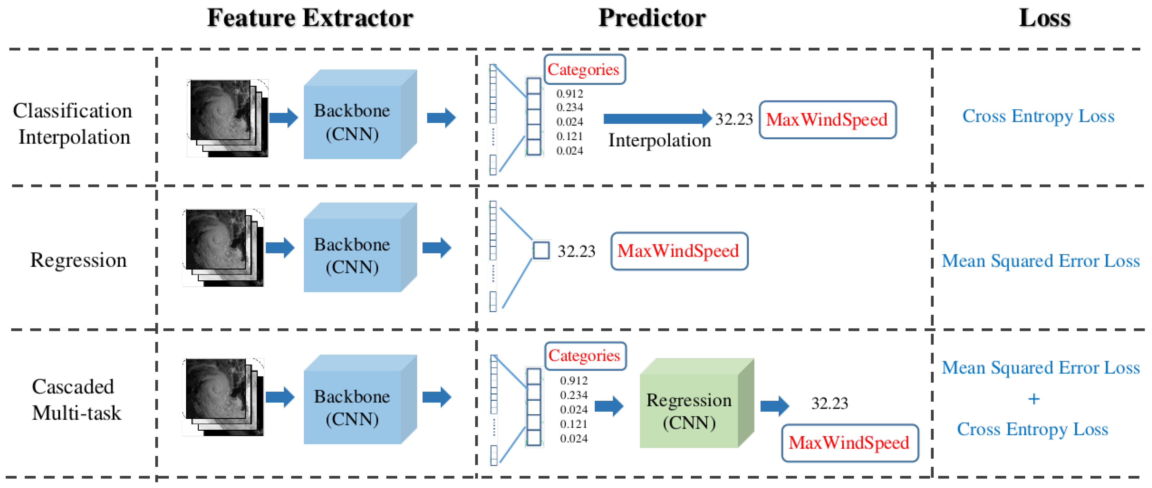In recent years, deep-learning-based intensity estimation models have been prospering and yielding promising results [9,10,11]. DL-based methods can be categorized into three types, as shown in Figure 1: (1) Classification-and-interpolation: Pradhan et al. [12] first proposed a deep CNN for categorizing TCs by estimating the wind speed through weighting the average of two highest categories with respect to their probabilities. Wang et al. [13] further improved the effect of intensity estimation by using a CNN with better feature extraction performance according to the idea proposed by Pradhan. (2) Regression: Recent studies [14,15,16] estimate TC intensity as a straightforward regression task and outperform the classification-and-interpolation method. (3) Multi-tasking: This school of methods usually cascades a classification model and a regression model. Considering that the intensity range of TCs is wide and a single regression model is insufficient for all kinds of TCs, Zhang et al. [17] proposed to use one classification model to divide the input image into three sub-classes and to then build three similar regression models to predict the max wind speed for each sub-class. Chen and Yu [18] proposed a practical multi-tasking architecture called Tensor CNN (TCNN) to perform intensity categorization and wind speed regression successively, which uses the trained classification model to ensure the afterward regression work’s accuracy. Both of the two multi-tasking methods’ idea is fundamentally to employ regression to estimate TC wind speed after intensity categorization, which does not take the relation of the TC categories and intensity into consideration naturally. These two methods mentioned above [17,18] only used the classification knowledge to restrict the regression model. Thus, the potential of the multi-task learning way has not been completely exploited yet. Exploring a new way of multi-task learning to bridge the gap between classification and intensity estimation is needed.

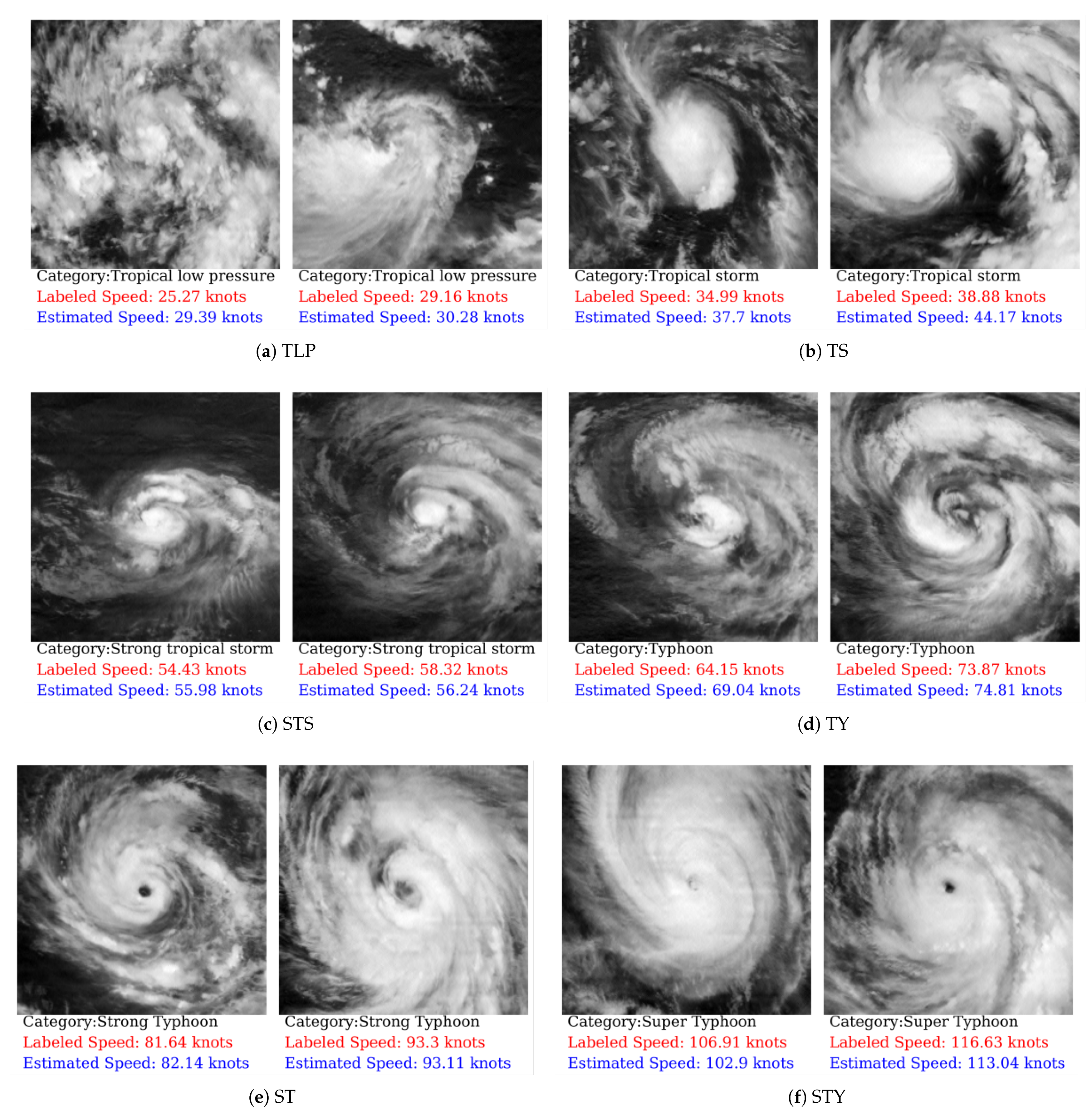
Furthermore, there are more challenges facing TC modeling. In nature, the numbers of different types of TCs are seriously unbalanced. The TCs in most of the obtained satellite images are of medium and low intensity, while there are few high-intensity TCs. And the intensity range of TCs ranges widely from 30 knots to more than 150 knots. Traditionally, the remote sensing community treats TC intensity and classification separately and ignores the correspondence between TC categorization and intensity. And the cascaded way of multi-task learning only employs the classification model to guide the subsequent regression models.

Aiming at fully leveraging the advantages of the multi-tasking method, we propose a parallel way of multi-tasking for TC classification and intensity estimation: Multi-Task Graph Residual Network (MT-GN). Our proposed model consists of two parts: feature extraction and task-dependency embedding. Both parts are trained in a parallel multi-tasking way, which is more reliable because of the method of sharing information between the two different tasks. Using a two-stage training method, we first train a residual CNN feature extractor from scratch. Then, after obtaining a fine feature map for the classification and estimation from this simple CNN structure, we drop the last fully connected layers, fix the feature extraction part, and only train the task-dependency embedding module. Consisting of two GCN layers, our task-dependency embedding module further improves our precision with a reweighting process.

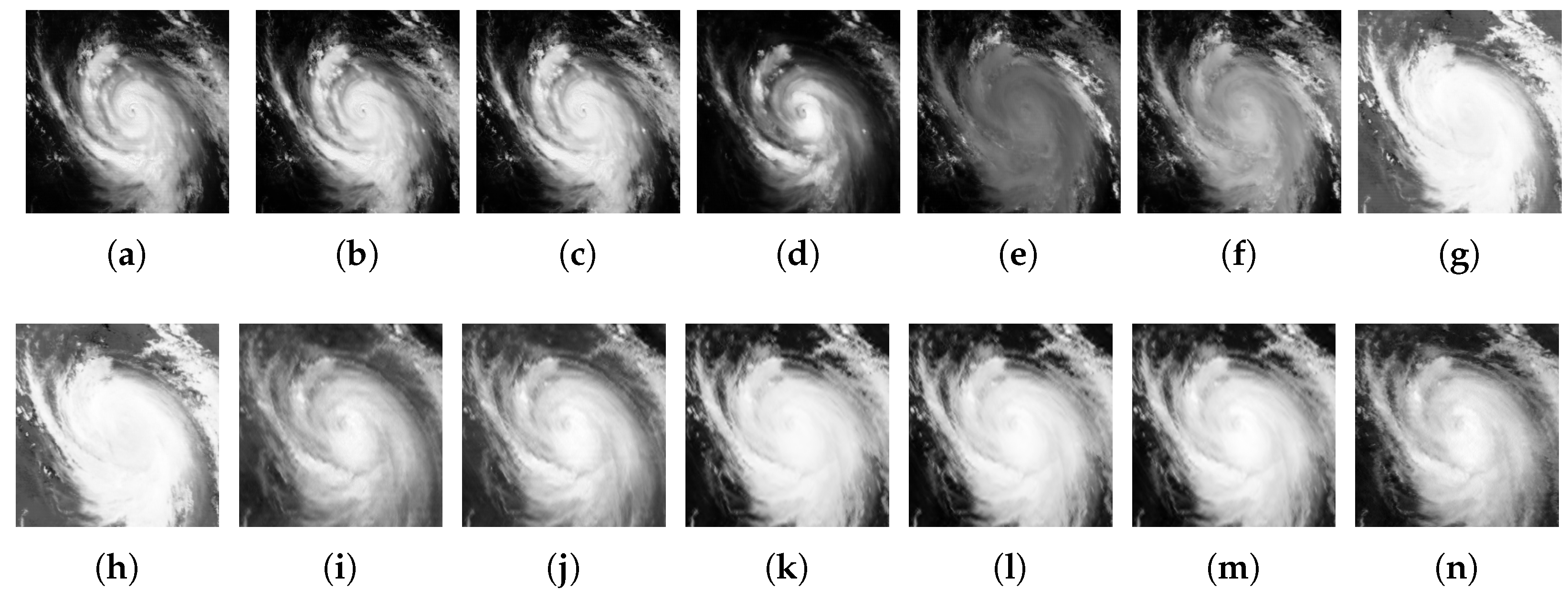
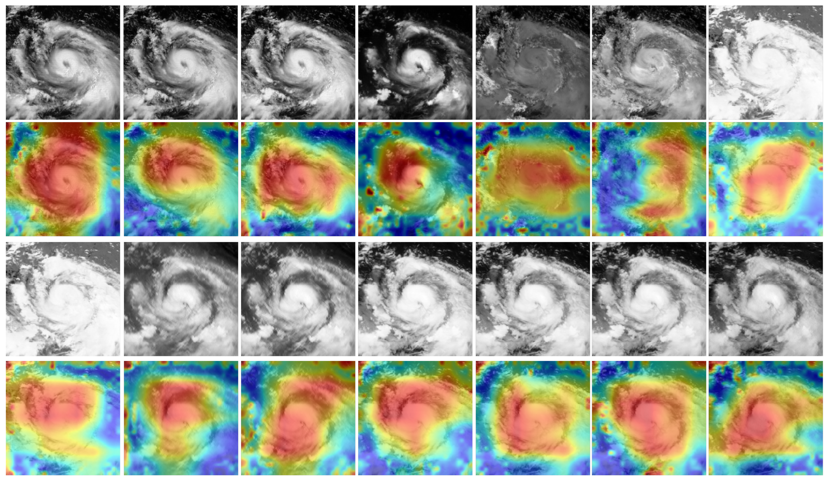
Further, we compared different feature extractors and input methods for multi-spectral images. Compared with infrared (IR) and water vapor (WV) images, using high-spectral-resolution multi-spectral data as input can provide more features and details of TCs. As high-dimensional data, multi-spectral images (MSIs) can cause the curse of dimensionality [19], and with visible bands (VIS), the MSIs captured during daytime and nighttime actually have 14 bands and 8 bands, respectively. Thus, studying different input methods for MSI to the CNN model is necessary. Moreover, using MSI obtained by China’s FY-4A satellite, we studied the channel-wise heatmap of multi-spectral images, which shines a light of understanding on the role of different channels of multi-spectral images in the TC deep learning field.

The main contributions provided in this work are as follows:

• We propose a parallel multi-tasking framework to classify TCs and estimate TC intensity simultaneously that has better performance than other methodologies under the comparison of the same dataset.
• Improvement of classification and estimation performance is achieved by a task-dependency embedding model based on a GCN.
• We improve the ability of the model using the residual modules and class balance loss to lay a solid foundation for prediction tasks.
• We constructed a multi-spectral benchmark dataset for tropical cyclone intensity estimation task using FY-4A multi-spectral data, which facilitates the fair comparison between different methodologies.

The rest of this article is organized as follows. Section 2 proposes the MT-GN for TC classification and intensity estimation, in which two modules, a feature extractor module and a task-dependency embedding module, are explained in full detail. Section 3 presents the details of our dataset, experiment setting, and results. The detailed analysis and discussion are listed in Section 4. Finally, Section 5 provides the conclusion.

2. Materials and Methods

2.1. Overall Framework

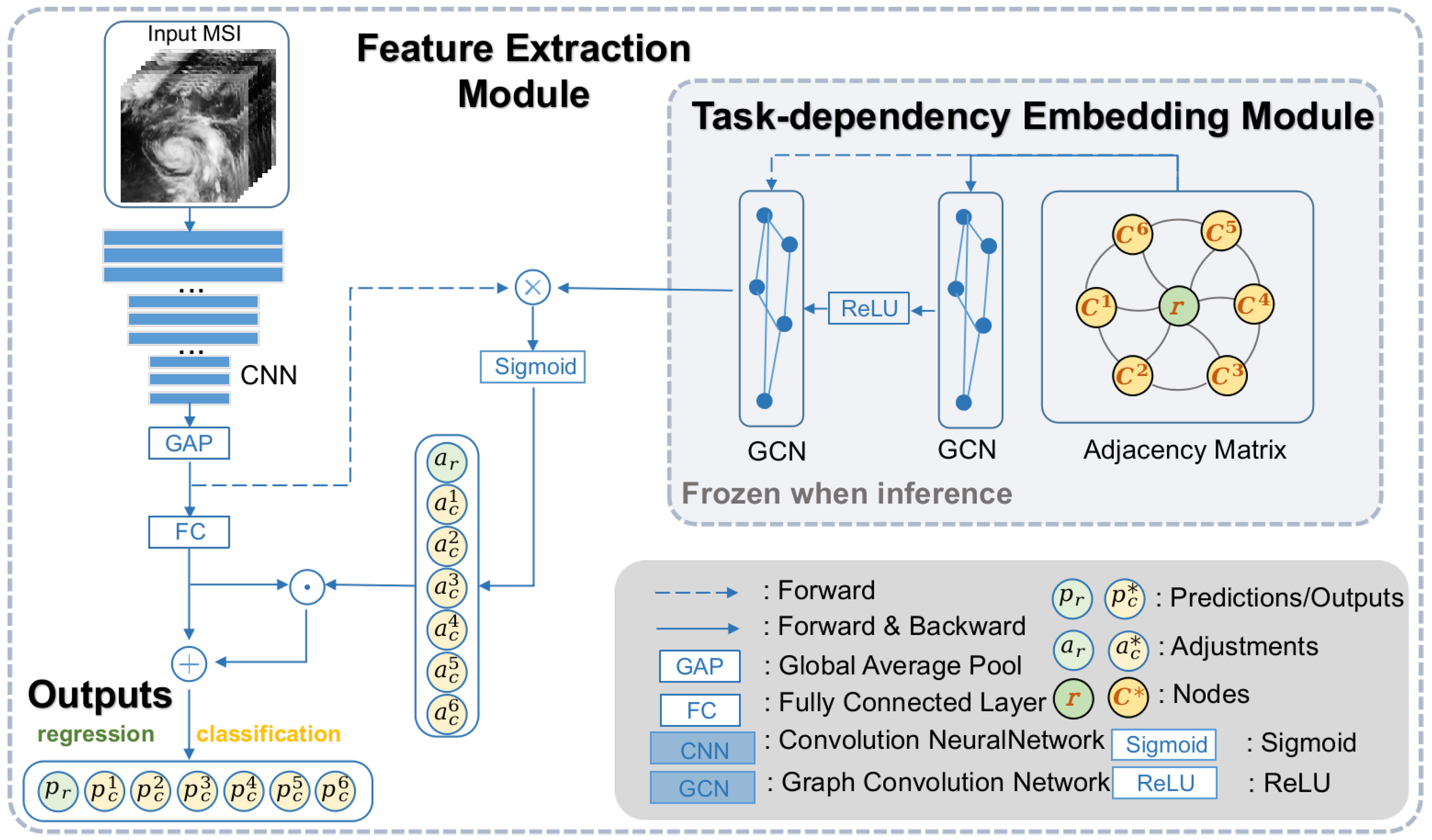
We illustrate the proposed parallel multi-task learning architecture MT-GN in Figure 2 as an overview. The input of our model is MSI image data, and the output is the predicted max wind speed and classification scores corresponding to the input. As shown in Figure 2, the left side is the CNN-based feature extraction module, and the right side is the GCN-based multi-task module. The r and $C^{\ast }$ nodes in the GCN module are embedded nodes corresponding to the GCN matrix, the green r node corresponds to the regression task, and the yellow $C^{\ast }$ nodes correspond to different categories in the classification task. Variables $a_r$ and $a_c^{\ast }$ are the adjustment vectors produced by the multi-task module, while $p_r$ and $p_c^{\ast }$ are the final outputs of the model.

The whole model follows a two-stage training strategy. First, we train the dual tasks of classification and regression on the CNN part, which includes a feature extraction backbone and a prediction layer (fully connected later). Then, a GCN-based task-dependency embedding module (TDEM) is introduced into our model. With the feature extraction backbone’s parameters frozen, the TDEM module takes the extracted feature map as input and learns the inter-task dependency knowledge to enhance the performance of multi-task prediction. Finally, in the evaluation stage, the MT-GN model formulates the inter-task dependency learned by the TDEM part as prior information to re-rank the original dual-task results predicted by the CNN part. The implementation details of our method are described in Section 2.2, Section 2.3 and Section 2.4.

2.2. Feature Extraction Module

In order to obtain better features, the depth of the neural network grows fast, which makes training deep CNNs difficult and lengthy. To overcome this problem, He et al. [20] introduces a residual module. Referring to it as the VGG19 network, He et al. [20] modifies the configuration of every layer and adds residual units through a short-circuit mechanism. An important design principle of ResNet [20] is that when the size of feature maps is reduced by half, the number of feature maps is doubled, which maintains the complexity of the network. To further reduce the number of parameters and matrix multiplications, He et al. [20] proposed a variant of the residual block that utilizes 1 × 1 convolutions to create a bottleneck. As shown in Figure 3, the bottleneck is composed of 1 × 1, 3 × 3, and 1 × 1 convolutions. The 1 × 1 convolution layer is used to reduce and restore dimensions. The 3 × 3 layer is used to integrate neighborhood information. With the shortcut connections in the convolution bottleneck in the CNN, the residual module can be used to reduce the number of parameters and increase the network depth efficiently.

Imitating the structure of ResNet and the bottleneck, we designed a feature extraction module as the basis of the network, which is composed of a convolution backbone and a fully connected prediction layer. After the extraction of CNN feature maps, we apply a global average pooling (GAP) layer before the fully connected layer [21]. With the GAP, we do not need to resize the input images to a fixed shape, which is often a required preprocessing cutting step for satellite images. The detailed structure of our feature extraction module is shown in

Table 1. Detailed configuration of the proposed CNN backbone.

Layer	Input Size	Output Size	Kernel Size
Conv1	14, 224, 224	64, 112, 112	7 × 7, 64, stride 2
MaxPool	64, 112, 112	64, 56, 56	3 × 3, stride 2
BottleNeck1	64, 56, 56	64, 56, 56	(C1 = 64, C2 = 64)@(3 × 3)
BottleNeck2	64, 56, 56	64, 56, 56	(C1 = 64, C2 = 64)@(3 × 3)
BottleNeck3	64, 56, 56	128, 56, 56	(C1 = 64, C2 = 128)@(3 × 3)
DownSample (Conv)	128, 56, 56	128, 28, 28	1 × 1, stride 2
BottleNeck4	128, 28, 28	128, 28, 28	(C1 = 128, C2 = 128)@(3 × 3)
BottleNeck5	128, 28, 28	256, 28, 28	(C1 = 128, C2 = 256)@(3 × 3)
DownSample (Conv)	256, 28, 28	256, 14, 14	1 × 1, stride 2
BottleNeck6	256, 14, 14	256, 14, 14	(C1 = 256, C2 = 256)@(3 × 3)
BottleNeck7	256, 14, 14	512, 14, 14	(C1 = 256, C2 = 512)@(3 × 3)
DownSample (Conv)	512, 14, 14	512, 7, 7	1 × 1, stride 2
BottleNeck8	512, 7, 7	512, 7, 7	(C1 = 512, C2 = 512)@(3 × 3)
GAP	512 × 7 × 7	512	7 × 7, stride 1
FC	512	7	512 × 7

.

During the first training stage, the whole feature extraction module along with its FC prediction layer is trained from scratch without the task-dependency embedding module. From the perspective of multi-task learning, the training of our feature extraction module is a hard parameter sharing technique in which the sharing layers are jointly optimized with multi-task supervisory signals. While in the second training stage, the proposed feature extraction module is kept fixed to maintain its strong feature extraction capability. With this multi-task feature extraction module, we can simultaneously tackle the TCs classification and intensity prediction tasks through a learned shared representation.

2.3. Task-Dependency Embedding Module

Although trained with two tasks’ labeled data, the CNN’s discriminative capability is still limited by the inconsistency between the two tasks. To mitigate this effect, we propose a task-dependency embedding module to adjust the network predictions through reweighting. The proposed task-dependency embedding module consists of two graph convolution layers with the ReLU activation function [22], which is trained with the image feature extraction modules’ parameters fixed. The detailed structure of the TDEM is demonstrated in Figure 2. With this GCN-based module, we can encode the graph structure of the feature maps directly and fit the prior relationship between the two tasks’ predictions.

As a branch of graph neural networks, a GCN performs similar operations as a CNN, which learns features from neighborhoods [23,24,25,26]. The key difference between a GCN and CNN is that the GCN is more general than the CNN and can handle unordered non-Euclidean data.

As introduced by [27], to perform semi-supervised classification, the output of a GCN is the probability of each prediction. Following Kipf and Welling [27], we denote the symmetric weighted adjacency matrix as A and the parameters of the two GCN layers as $W_1$ and $W_2$. And $J_{c\left(i\right)}$ represents for classification score adjustment for the i-th category, and $J_r$ represents the regression adjustment. In our TDEM module, the graph structure embedded by the GCN formulates the regression adjustment $J_r$ and the classification scores adjustment $J_{c\left(i\right)}$ as independent nodes, which models the relationship between different nodes via a relationship matrix $\widehat{A}\in {\mathbb{R}}^{N\times N}$, where N represents the number of output nodes. Taking both the CNN features X and the adjacency matrix A as inputs, the TDEM produces the learned relationship matrix $\widehat{A}$ and adjustment output $J_{\ast }$. The initial input feature X is the output of the CNN’s GAP layer, while the input feature of the second GCN layer is the output feature of the first GCN. Through backpropagation, the learned adjacency matrix $\widehat{A}$ in a GCN can represent the dependencies of two tasks in the feature space. The values in the adjacency matrix measure the corresponding correlation between prediction nodes.

To sum up, the whole process of the TDEM module is as follows: first, obtain the feature vector X obtained by the GAP layer and calculate the relationship matrix $\widehat{A}$ of the graph structure by the adjacency matrix A; then, input them into a two-layer GCN network to obtain the prediction nodes J. Our forward calculation takes the form:

$$J=f(X,A)=Softmax\left(\widehat{A}ReLU\left(\widehat{A}X{W}_1\right)W_2\right)$$

(1)

Here, $W_1\in {\mathbb{R}}^{C\times H}$ is an input-to-hidden weight matrix for a hidden layer with H feature maps. $W_2\in {\mathbb{R}}^{H\times S}$ is a hidden-to-output weight matrix. And the relationship matrix $\widehat{A}$ is defined as $\widehat{A}={\tilde{D}}^{-\frac{1}{2}}\tilde{A}{\tilde{D}}^{-\frac{1}{2}}$, with $\tilde{A}=A+I_N$ and ${\tilde{D}}_{ii}={\sum }_j{\tilde{A}}_{ij}$.

Finally, we apply the output $J\in {\mathbb{R}}^{N\times N}$ of the TDEM to the original output $F_{org}\in {\mathbb{R}}^{N\times 1}$ of the FC layer of the feature extraction module in an element-wise manner as a weighted adjustment. The reweighting process can be written as follows:

$$F_{final}=Softmax\left(J\odot F_{org}+F_{org}\right)$$

(2)

Here, $F_{final}$ denotes the final prediction result of our MT-GN network. In this way, we integrate the task-dependency prior to the following prediction part of the model.

2.4. Loss Function

Traditionally, classification and regression tasks are tackled in isolation, i.e., a separate neural network is trained for each task. Unlike the traditional learning way, multiple tasks are solved jointly in multi-task learning (MTL), and inductive bias is shared between the tasks [28,29,30,31]. MTL can be formulated as a weighted minimization problem as:

$$\underset{\begin{array}{c}{\theta }^{sh}\\ {\theta }^1,\dots ,{\theta }^T\end{array}}{min}\sum _{t=1}^T{c}^t{\widehat{\mathcal{L}}}^t\left({\theta }^{sh},{\theta }^t\right)$$

(3)

where $c^t$ demonstrates the predefined or dynamic weights for the t-th task, and ${\widehat{\mathcal{L}}}^t$ represents the empirical loss of the t-th task, which is defined by Equation (4):

$${\widehat{\mathcal{L}}}^t\left({\theta }^{sh},{\theta }^t\right)=\frac{1}{N}\sum _i\mathcal{L}\left(f^t\left({\mathbf{x}}_i;{\theta }^{sh},{\theta }^t\right),y_i^t\right)$$

(4)

In the above equation, N represents the number of sample for the t-th task, $f^t$ represents the network model for the t-th task, ${\theta }^{sh}$ represents the model parameters shared among multiple tasks, ${\theta }^t$ represents the exclusive model parameter of the t-th task, and $y_i^t$ represents the label for the i-th sample of the t-th task.

For our multi-task learning model, we design a mixed loss function. For the regression part, we use the mean squared loss. For the classification part, we choose a class-balanced loss. Because the distribution of TC categories is very uneven, previous studies usually apply manual oversampling or downsampling to the datasets. However, upsampling simply expands the dataset by rotation and additional noise in order to replicate small class samples [6]. The characteristics of the new data are highly similar to the original data, and there is no essential performance improvement. Downsampling reduces the performance of the model for major categories. Neither of them introduce the prior knowledge of the relative quantity of different categories. Therefore, we use the class-balanced loss function based on the relative number of classes [32]. Finally, we use the weighted sum method to balance the two sub-parts of the mixed loss function. Our mixed loss function $\mathcal{L}$ formula is as follows:

$$\mathcal{L}={\mathcal{L}}_{reg}+\lambda {\mathcal{L}}_{\mathrm{cls}}$$

(5)

Here, ${\mathcal{L}}_{reg}$ and ${\mathcal{L}}_{cls}$ represent the loss function for regression and classification, respectively, and $\lambda$ denotes the weight of the classification part. The following equations formulate the details of the two loss functions:

$${\mathcal{L}}_{reg}={\left(Y_{reg}-F_{reg}^{\ast }\right)}^2$$

(6)

$${\mathcal{L}}_{cls}\left(i\right)=-\frac{1-\beta }{1-{\beta }^{n_i}}\sum _{j=1}^C{\left(1-F_{cls,j}^{\ast }\right)}^{\gamma }log\left(F_{cls,j}^{\ast }\right)$$

(7)

where $Y_{\ast }$ represents the label for regression or classification, $F^{\ast }$ represents the original output of the CNN part of the final output adjusted by the GCN part, $n_i$ represents the number of samples of category i, C represents the number of categories, and $\beta$ and $\gamma$ are hyperparameters in the loss function.

It is worth noting that the GCN network weights $W_1$ and $W_2$ are trained with the same loss function and learning rate as the CNN part. Thus, we obtain a simple yet consistent training scheme for the two parts of the model.

3. Experiment and Results

3.1. Dataset and Evaluation Metrics

In this paper, we constructed a benchmark dataset based on FY-4A image and best-track data to fairly compare the advantages and disadvantages of different methods. All models for TC classification and intensity estimation in this study are evaluated on this benchmark. We publish our benchmark dataset online for the convenience of reproduction and follow-up research (https://randomless.github.io/FY4A-TC-Benchmark/ (accessed on 11 November 2023)).

3.1.1. FY-4A Satellite Data and TC Data

To build our benchmark dataset, we collected the data of FY-4A and TCs over the southeast coast of China and the northwest Pacific from 2018 to 2021, which were provided by the Shanghai Meteorological Bureau, Shanghai, China.

Launched in December 2016, China’s FY-4A meteorological satellite carries an Advanced Geosynchronous Radiation Imager (AGRI), which can provide high-quality images of the cyclones over the northwest Pacific Ocean. We construct our dataset with the multi-spectral images of the FY-4A/AGRI. The central wavelengths and the names of the bands are displayed in

Table 2. Instrument specifications for FY-4A/AGRI sensor.

Band	Central Wavelength (μm)	Band Name
1	0.47	Blue Band
2	0.65	Red Band
3	0.83	Veggie Band
4	1.37	Cirrus Band
5	1.61	Snow/Ice Band
6	2.22	Cloud Particle Size Band
7	3.72	Shortwave Window Band—High
8	3.72	Shortwave Window Band—Low
9	6.25	Upper-Level Tropospheric Water Vapor Band
10	7.1	Lower-Level Water Vapor Band
11	8.5	Cloud-Top Phase Band
12	10.8	Clean IR Longwave Window Band
13	12	Dirty Longwave Window Band
14	13.5	CO2 Longwave Infrared Band

.

The best-track data of TCs are obtained from the China Meteorological Administration (CMA) (https://tcdata.typhoon.org.cn/ (accessed on 11 November 2023)). The CMA TC best-track dataset covers TCs that develop over the northwestern Pacific Ocean. The basin is to the north of the equator and to the west of 180°E and includes the South China Sea (SCS). The data contain the central location (latitude/longitude) of TCs as well as the maximum wind speed (MWS) and typhoon category, which is provided every 3 or 6 h. Depending on the wind speed, dissipation power index, integrated kinetic energy index, and storm severity index, TCs are graded into six classes according to the TC intensity classification standard of the China Tropical Cyclone Classification Standard, GBT 19201-2006 [33]. The typhoon categories and corresponding wind speed ranges are shown in

Table 3. Classification of cyclone categories and corresponding wind scales.

No.	Category	Abbreviation	Wind Speed (knots)	Wind Speed (m/s)
1	Tropical low pressure	TLP	20.99–33.24	10.8–17.1
2	Tropical storm	TS	33.25–46.64	17.2–24.4
3	Strong tropical storm	STS	46.65–61.22	24.5–32.6
4	Typhoon	TY	61.23–79.68	32.7–41.4
5	Strong Typhoon	ST	79.69–99.12	41.5–50.9
6	Super Typhoon	STY	≥99.13	≥51.0

.

3.1.2. Benchmark Dataset Construction

The TC image extraction process based on FY-4A data is shown in Figure 4. The construction steps for the benchmark dataset are as follows:

(1)

TC Data Matching: Because the time resolution of TC data is inconsistent with that of FY-4A image data, we match the best-track data with the image data.

(2)

Image Cropping: As the raw FY-4A image data contain the entire half-disk area, we need to further crop the image data according to the TC data. The maximum wind speed, longitude, and latitude data in TC data are linearly interpolated to the same time resolution as FY-4A image data. Then, based on the longitude and latitude of the TC center at the corresponding time, we select the surrounding 240 × 240 pixel area as the TC sample at that time. The values of the TC sample’s classification and intensity label are assigned based on the interpolated TC data. Thus, a constructed TC sample includes 240 × 240 image data for 14 channels, maximum wind speed in knots, and category labels. Examples of the cropped images are shown in Figure 5 and Figure 6.

(3)

Normalization: In order to accelerate model weight convergence, normalization is applied to every MSI image. The pixel value in every normalized channel of the satellite image data ranges from [0,1].

(4)

Dataset Split: After obtaining the constructed TC samples, we divide all of them into the training set and test set according to a ratio of 8:2. It is worth noting that the TC instances of the training set and the test set do not intersect each other after the division. In addition, using the geometric properties of TCs, we rotated the samples in the training set by 90° and 180° to expand the training set. The training set is used for parameter learning and tuning, while the test set is used for performance evaluation.

Figure 5. Day images of a cyclone sample cropped from the original FY-4 MSIs: (a) 1st, (b) 2nd, (c) 3rd, (d) 4th, (e) 5th, (f) 6th, (g) 7th, (h) 8th, (i) 9th, (j) 10th, (k) 11th, (l) 12th, (m) 13th, and (n) 14th band.

Figure 5. Day images of a cyclone sample cropped from the original FY-4 MSIs: (a) 1st, (b) 2nd, (c) 3rd, (d) 4th, (e) 5th, (f) 6th, (g) 7th, (h) 8th, (i) 9th, (j) 10th, (k) 11th, (l) 12th, (m) 13th, and (n) 14th band.

Figure 6. Night images of a cyclone sample cropped from the original FY-4 MSIs: (a) 1st, (b) 2nd, (c) 3rd, (d) 4th, (e) 5th, (f) 6th, (g) 7th, (h) 8th, (i) 9th, (j) 10th, (k) 11th, (l) 12th, (m) 13th, and (n) 14th band.

Figure 6. Night images of a cyclone sample cropped from the original FY-4 MSIs: (a) 1st, (b) 2nd, (c) 3rd, (d) 4th, (e) 5th, (f) 6th, (g) 7th, (h) 8th, (i) 9th, (j) 10th, (k) 11th, (l) 12th, (m) 13th, and (n) 14th band.

Finally, a total of 5442 satellite images of TCs are selected to train the proposed model, and 939 images of TCs were selected to verify the performance of the models. We use knots as the unit for wind speed to facilitate easier comparison with other research, but we also provide m/s versions in all of the experimental results tables.

Besides taking all 14 channels of image data as input, we also produce more forms of input image data for the TC samples. Considering the input bands, Dawood et al. [34] and Zhang [6] take the IR channel as input; Zhang [17] and Lee [16] take the IR and water vapor channels as input. Therefore, in order to make an approximate comparison with them, we further processed the FY-4A multi-channel data. According to the central wavelength of the band, we select the 12th band as the single-channel input for IR and select the 7th, 9th, 12th, and 13th bands as the four-channel input for IR and WV. In addition, we also perform dimensionality reduction on 14-channel FY-4A data through principal component analysis (PCA) to get statistical information from multi-channel images. By setting the principal component numbers of the PCA to one and four, we obtain the settings of PCA1 and PCA4 for the model’s input. See Section 4.2 for the corresponding comparison experiment.

Additionally, according to the acquisition times of images, we further divide image data into daytime and nighttime data. The time period of daytime data is from 21:01 of the previous day to 08:59 of the current day (UTC). The time period of nighttime data is 09:00–21:00 (UTC) of the current day. For daytime data, we can use all of the FY-4A/AGRI bands (14 bands). As for nighttime data, since the VIS band cannot obtain data at night, the nighttime data can be studied by using all bands 1–14 or by using infrared bands 8–14. See Section 4.2 for a specific comparative study between daytime and nighttime.

3.1.3. Evaluation Metrics

To compare the results of classification and intensity estimation, we evaluate the models’ performances using various statistical indices. For the classification task, we employ multiple indices, including Top-2 accuracy, Kappa coefficient (Kappa), precision, recall, and F1-score. For TC intensity estimation (max wind speed regression), we mainly use absolute error (MAE), mean-square error (MSE), and root-mean-square error (RMSE) as evaluation metrics. For a more detailed study on the difference between the best-track data and the estimated intensity of each category, we also apply bias, overestimation rate, and underestimation rate as complementary metrics. The computation formula for our complementary metrics is demonstrated as follows, where $Y_{reg}$ represents the label of the regression, and $F_{reg}$ represents the output of the model.

$$\mathrm{Bias}=\frac{1}{n}\ast \sum \left(Y_{reg}-F_{reg}\right)$$

(8)

$$\mathrm{Overestimation}\mathrm{Rate}=\frac{number(Y_{reg}<F_{reg})}{number\left(Y_{reg}\right)}\ast 100\%$$

(9)

$$\mathrm{Underestimation}\mathrm{Rate}=\frac{number(Y_{reg}>F_{reg})}{number\left(Y_{reg}\right)}\ast 100\%$$

(10)

3.2. Setup

All of the models for comparison were trained from scratch using the PyTorch framework (in Python 3.7) running on a computer with four NVIDIA TITAN Xp (Pascal) GPUs. All experiments employed the same data preprocessing method, which ensures that the comparison between models is fair. The batch size for training was 128, the learning rate was 0.001, and the training procedure ends at the 24th epoch. As for the update scheduler of the learning rate, cosine annealing is employed in all experiments. We used the Adam optimizer to optimize the loss function with hyperparameters $\beta 1$ and $\beta 2$ set as 0.90 and 0.99, respectively. Furthermore, the best-performing model on the test dataset is evaluated and saved during the optimization process. For our proposed MT-GN method, a two-stage training process is implemented according to Algorithm 1.

Algorithm 1 Two-stage training process and inference process of MT-GN.

TRAIN:  (Feature Extraction Module) 1: Initialize the parameters ${\theta }_{cnn}$ of the CNN part randomly. 2: while ${\theta }_{cnn}$ not converged do 3:    Compute loss $\mathcal{L}$ by Equations (5)–(7). 4:    Update ${\theta }_{cnn}$ with loss $\mathcal{L}$ by Adam optimizer. 5: end while TRAIN:  (Task-dependency Embedding Module) 6: Initialize the parameters ${\theta }_{gcn}$ of the GCN part randomly; freeze ${\theta }_{cnn}$. 7: while ${\theta }_{gcn}$ not converged do 8:    Compute loss $\mathcal{L}$ by Equations (5)–(7). 9:    Update ${\theta }_{gcn}$ with loss $\mathcal{L}$ by Adam optimizer. 10: end while PREDICT:  (MT-GN Model) 11: Freeze the parameters ${\theta }_{gcn}$. 12: Predict the final output of classification and regression $F_{cls}$, $F_{reg}$ by Equation (2).

3.3. Results of Different Models

In order to illustrate the advantages and performance of our proposed parallel multi-tasking architecture, we design a cascaded multi-tasking model similar to TCICENet, a direct regression model similar to Deep PHURIE, and a classification-and-interpolation model similar to Deep CNN. All models use the same feature extractor backbone and neural network operators, with only the architecture of the networks being different. We use four different CNN backbones as feature extractors to compare the classification accuracy and regression accuracy of these four methods. Among them, the classification results of the regression method are directly obtained from the predicted wind speed according to the wind speed range in Table 3. In addition, we also draw the scatter diagrams of wind speed bias of the four methods and the box diagrams of bias by category of the classification results of the four methods based on Res-2D-CNN, as shown in Figure 7 and Figure 8, respectively. In the scatter diagrams, we also draw the fitting line and show the Pearson correlation coefficient (PCC) and R-squared value ($R^2$) between the predicted wind speed and the labeled wind speed to intuitively measure the accuracy of wind speed prediction.

The results in

Table 4. Classification and intensity estimation performance comparison for different backbones and methodologies.

Backbone	Methodologies	Top-2 Accuracy (%)	F1-Score	MAE	RMSE	Bias	Overestimation Rate (%)	Underestimation Rate (%)
2D-CNN	classification + interpolation	74.84	0.41	11.62	15.21	−5.74	76.86	23.14
	regression	74.32	0.44	9.21	12.21	−1.95	71.51	28.49
	cascaded multi-task	78.07	0.54	8.54	11.66	0.67	54.7	45.3
	parallel multi-task (MT-GN)	79.50	0.57	8.47	11.31	1.3	55.91	44.09
Res-2D-CNN	classification + interpolation	85.51	0.49	10.22	13.36	−5.55	71.54	28.46
	regression	86.56	0.52	7.77	10.39	−1.75	62.58	37.42
	cascaded multi-task	90.15	0.61	7.19	9.74	0.86	46.06	53.94
	parallel multi-task (MT-GN)	90.37	0.64	7.06	9.50	1.52	46.59	53.41
3D-CNN	classification + interpolation	75.15	0.43	11.47	14.91	−5.74	79.01	20.99
	regression	76.07	0.46	8.97	11.83	−1.93	71.5	28.5
	cascaded multi-task	79.16	0.54	8.27	11.34	0.68	53.55	46.45
	parallel multi-task (MT-GN)	81.18	0.58	8.28	11.14	1.36	55.59	44.41
Res-3D-CNN	classification + interpolation	79.97	0.46	10.81	14.24	−5.65	75.96	24.04
	regression	82.23	0.48	8.57	11.19	−1.86	66.88	33.12
	cascaded multi-task	85.45	0.57	7.94	10.79	0.76	51.08	48.92
	parallel multi-task (MT-GN)	85.49	0.60	7.66	10.36	1.4	51.85	48.15

demonstrate that our proposed method improves both classification and regression accuracy and performs favorably against state-of-the-art approaches. In contrast, two multi-tasking methods can obtain more accurate results than the classification-and-interpolation method and regression method, no matter what kind of feature extractor is used.

It can be seen from Figure 7a–d that the values of PCC and $R^2$ of the two multi-tasking methods are significantly higher those the other two methods. Among them, the classification-and-interpolation method is the worst, and its R-squared value is only 0.755, while the parallel method is the best, and its R-squared value is 0.8492. The R-squared values of the cascaded method and regression method are 0.8408 and 0.8210, respectively. Intuitively, the scatter points in Figure 7c,d are more concentrated near the fitting curve. This is mainly because the multi-task learning method introduces more supervisory information into the whole neural network, while the classification and regression methods only take one kind of supervisory information into consideration. Compared to the two multi-task learning methods, the overall performance of our parallel multi-tasking method is comparable to the performance of the cascaded multi-tasking method with the same backbone setting. On the whole, the intensity estimation results of the parallel method are better than those of the cascaded method using different backbones. When Res-2D-CNN is used, the RMSE of the parallel method is 9.50 knots, which is lower than that of the cascaded method (9.74 knots).

For the two methods that adopt a single kind of supervision information, the accuracy of the regression method is better than that of the classification-and-interpolation method. The classification-and-interpolation method is the first proposed method of the four methods. It only considers the direct weighted interpolation of classification scores to obtain the wind speed, which is simple and rough. It can be seen from Figure 7a that the scatter points of the classification-and-interpolation method are more discrete, indicating that the model cannot predict the wind speed close to the true value well. In Figure 8a, the classification-and-interpolation method has a wider error range for different TC categories, especially TY, ST, and STY.

In addition, four different convolutional backbones are compared in Table 4. From the accuracy comparison in the table, it can be seen that the quality of the feature extraction convolutional backbones adopted by the model significantly affects the final performance of the model. Taking the parallel multi-tasking method we proposed as an example, the Top-2 accuracy of Res-2D-CNN is 10.87%, 9.19%, and 4.88% higher than that of 2D-CNN, 3D-CNN, and Res-3D-CNN, respectively, and the MRSE is reduced by 1.81, 1.64, and 0.86 knots, respectively. This shows that for the problem of TC classification and intensity estimation, developing an effective feature extractor for TC can significantly improve the accuracy of the model. On the whole, Res-2D-CNN shows the advantage of the residual structure for improving the feature extraction effect of convolution layers. However, the performance of the two 3D-CNN-based backbones is worse than that of the two 2D-CNN-based backbones. This may be because 3D-CNN cannot effectively learn 14-channel MSI data. In the future, we can consider adding channel attention mechanics to 3D-CNN to improve the feature extraction performance of the 3D-CNN layers.

For the inference procedure, our parallel multi-tasking method can output the classification results and intensity estimation results only by inference the model once, while the other three methods need two-step inference. The classification-and-interpolation method needs to interpolate the classification results to predict the wind speed, the regression method produces the classification results according to the wind speed range, and the cascaded multi-tasking method needs to use two CNN networks to predict the classification and regression results in two steps. And as shown in the above discussion, using the same backbone network for a fair comparison, our parallel multi-tasking method has similar accuracy to that of the SOTA cascaded multi-tasking method. In summary, our proposed parallel multi-tasking method is a promising TC classification and intensity estimation technique that has great developmental potential.

4. Analysis and Discussion

4.1. Other Satellite-Based Methods Comparison

In order to verify the performance of our model, it was compared with the existing TC classification models and intensity estimation models listed in

Table 5. Comparison of classification performance on 14-channel FY-4A data.

Model	Top-2 Accuracy (%)	F1-Score	Precision (%)	Recall (%)	Kappa
kNN	66.05	0.42	0.51	0.29	0.25
SVM	68.89	0.39	0.39	0.25	0.21
MLR	81.83	0.46	0.45	0.29	0.25
ANN	81.59	0.44	0.41	0.26	0.22
MT-GN	90.37	0.57	0.64	0.39	0.36

and Table 6. Using our FY-4A benchmark dataset, the performance of intensity estimation between our model and other models—DAVT, Deep CNN, DeepMicroNet, M16, ETCI, CNN-TC, MLR, TCIENet, Transfer-VGG19, 3D-CNN, Deep PHURIE, TCICENet, and T-TCNN—was compared. The performance of classification between our model and other models—k-Nearest Neighbor (kNN), Support Vector Machine (SVM), Multiple Linear Regression (MLR), and Artificial Neural Network (ANN)—was compared.

Table 5 shows the comparison of TC classification between our method and several traditional methods on our benchmark dataset. Top-2 accuracy, precision, recall, F1-score, and Kappa were utilized to evaluate the performance of the models in Table 5. It can be seen from the table that the classification accuracy of our GT method is much higher than those of the traditional methods. Compared with kNN, SVM, MLR, and ANN, our MT-GN yields decent accuracy for each category. High recall, precision, and F1-score indicate that MT-GN can identify the intensity categories with fewer missed alarms and fewer false alarms.

Table 6 demonstrates a rough comparison between the RMSEs and MAEs of TC intensity estimation of our proposed MT-GN and other satellite-based works. It can be seen from Table 6 that all learning-based methods are superior to traditional methods. The traditional technique DAVT not only needs manual intervention, but the RMSE is only 19.01 knots. Whilst the feature extractor and input data of the model are different, the final output of the classification-and-interpolation models is the probability of the category, not the maximum wind speed. The estimated intensity is subsequently determined as the weighted average of the several categories that have high probabilities. Although classification-and-interpolation methods exhibited good performance in TC intensity estimation, compared with the regression methods, the performance of these models still has a large amount of room for improvement. The intensity estimation results based on regression methods were generally better than the results of classification-and-interpolation methods.

Strictly speaking, it is not fair to directly compare these learning-based models [6,12,13,15,16,17,18,34,35,36,37,38] due to the use of different datasets. Especially in the T-TCNN [18] paper, the division of the training set and test set is also different from that of other papers. Every existing research article has adopted its own independent dataset that focuses on different bands of different sensors, e.g., infrared [12,13], water vapor [17], SWIR [16], and microwave data [35]). There is no unified standard dataset to fairly measure the pros and cons of these models. In addition, these learning-based methods use different feature extractors (that is, the CNN part), which makes it more difficult to compare among various studies. In our study, as mentioned in Section 2 and Section 3, we used the same CNN backbone for a fair comparison of methods of different schools on the benchmark dataset constructed from the MSI satellite images and the subset of MSI bands, which provides the possibility for further in-depth and effective research on TC classification and intensity estimation tasks.

Table 6. Comparison of RMSEs and MAEs for TC intensity estimation: our proposed MT-GN vs. other satellite-based approaches.

Model	Methodology	Data	RMSE (knots)	MAE (knots)	Reference
DAVT	traditional/statistical analysis	IR	19.01	16.64	[39]
Deep CNN	classification + interpolation	IR	12.95	10.12	[12]
DeepMicroNet	classification + interpolation	MINT	10.60	—	[35]
M16	classification + interpolation	IR	10.04	—	[13]
ETCI	classification + interpolation	IR	16.34	14.03	[36]
CNN-TC	regression	IR, PMW	10.38	—	[15]
MLR	regression	IR	16.21	14.88	[37]
TCIENet	regression	IR, WV	9.98	7.84	[17]
Transfer-VGG19	regression	IR	13.23	—	[38]
3D-CNN	regression	SWIR, WV, IR	11.34	8.65	[16]
Deep PHURIE	regression	IR	10.55	8.37	[34]
TCICENet	cascaded multi-task	IR	9.59	7.45	[6]
T-TCNN	cascaded multi-task	MSI	3.75	3.13	[18]
MT-GN	parallel multi-task	IR	8.96	8.02	This study
MT-GN	parallel multi-task	IR1, IR2, WV, SWIR	8.63	7.72	This study
MT-GN	parallel multi-task	PCA1	10.41	8.02	This study
MT-GN	parallel multi-task	PCA4	9.08	7.50	This study
MT-GN	parallel multi-task	MSI	9.50	7.06	This study

Table 6. Comparison of RMSEs and MAEs for TC intensity estimation: our proposed MT-GN vs. other satellite-based approaches.

Model	Methodology	Data	RMSE (knots)	MAE (knots)	Reference
DAVT	traditional/statistical analysis	IR	19.01	16.64	[39]
Deep CNN	classification + interpolation	IR	12.95	10.12	[12]
DeepMicroNet	classification + interpolation	MINT	10.60	—	[35]
M16	classification + interpolation	IR	10.04	—	[13]
ETCI	classification + interpolation	IR	16.34	14.03	[36]
CNN-TC	regression	IR, PMW	10.38	—	[15]
MLR	regression	IR	16.21	14.88	[37]
TCIENet	regression	IR, WV	9.98	7.84	[17]
Transfer-VGG19	regression	IR	13.23	—	[38]
3D-CNN	regression	SWIR, WV, IR	11.34	8.65	[16]
Deep PHURIE	regression	IR	10.55	8.37	[34]
TCICENet	cascaded multi-task	IR	9.59	7.45	[6]
T-TCNN	cascaded multi-task	MSI	3.75	3.13	[18]
MT-GN	parallel multi-task	IR	8.96	8.02	This study
MT-GN	parallel multi-task	IR1, IR2, WV, SWIR	8.63	7.72	This study
MT-GN	parallel multi-task	PCA1	10.41	8.02	This study
MT-GN	parallel multi-task	PCA4	9.08	7.50	This study
MT-GN	parallel multi-task	MSI	9.50	7.06	This study

4.2. Input Comparison

As for the comparison of input bands, we train the MT-GN with seven different input forms. We select the 12th channel of FY-4A as the single-channel input, named IR, and the 7th, 9th, 12th, and 13th channels of FY-4A as the four-channel input, named IR1, IR2, WV, and SWIR. Corresponding to a single channel and four channels, we use principal component analysis technology to extract two types of principal components from 14-channel cropped images: one is single-channel PCA1, and the other is four-channel PCA4. In addition, we divide the original MSI data into daytime and nighttime as input data according to time; these categories are named Day and Night, respectively. We use the same parameters and model settings for each input dataset. After the iteration of 24 epochs for these MT-GN models, the losses reached their minimum, and the accuracies of the intensity estimation reached their maximum.

The impacts of input form on the performance of the MT-GN are presented in

Table 7. Comparison of classification and intensity estimation performance using different inputs.

Input Channel	Channel Number	Top-2 Accuracy (%)	F1-Score	MAE	RMSE	Bias	Overestimation Rate (%)	Underestimation Rate (%)
IR	1	88.17	0.57	8.02	8.96	2.19	41.69	58.31
IR,WV	4	89.15	0.6	7.72	8.63	1.49	39.47	60.53
PCA1	1	83.36	0.51	8.02	10.41	2.2	41.4	58.6
PCA4	4	89.45	0.53	7.5	9.08	0.7	41.52	58.48
MSI	14	90.37	0.64	7.06	9.5	1.52	46.59	53.41
Day	14	75.08	0.43	10.15	12.51	4.12	31.27	68.73
Night	8	82.96	0.4	8.89	11.24	3.85	37.24	62.76

. The Top-2 accuracy of IR input is 88.17%, whereas the Top-2 accuracy of IR1, IR2, WV, and SWIR can reach approximately 89.15%. The accuracy of TC classification and intensity estimation of PCA4 is higher than that of MSI. However, the accuracy of classification and intensity estimation is relatively low when the input is PCA1. This demonstrates that relatively satisfactory results can still be obtained using only infrared channel data or four artificially selected channels for TC classification and intensity estimation tasks.

It can also be seen from Table 7 that due to the split training data, the accuracy of Day and Night is lower than that of MSI as a whole, and the classification accuracy and intensity estimation accuracy of Day is lower than that of Night. This may be because the Night input only adopts the input of the infrared part of the last eight channels of FY-4A, which reduces the impact of noise in the visible bands.

4.3. Category Comparison

As mentioned above, the TC intensity grade is divided into a total of six categories. In this section, we focus on the performance of TC classification and intensity estimation for all six categories individually. The results for these categories are listed in

Table 8. Comparison of intensity estimation performance for all TC categories.

Model	Category	MAE	RMSE	Bias	Overestimation Rate (%)	Underestimation Rate (%)
MT-GN	TLP	4.48	6.02	−3.09	73.74	26.26
	TS	6.33	7.7	2.51	30.55	69.45
	STS	7.21	9.29	7.74	24.77	75.23
	TY	6.67	10.08	3.17	44.44	55.56
	ST	7.57	11.49	6.46	26.53	73.47
	STY	7.97	11.16	7.41	24.56	75.44
	Avg	7.06	9.50	1.52	46.59	53.41

.

For intensity estimation, the mean MAEs of all six categories are below 7.06 knots. The RMSEs from weak to strong intensity for the six TC categories are 6.02, 7.70, 9.29, 10.08, 11.49, and 11.16 knots, respectively. It can be seen that the results of the model are satisfactory for all categories. Figure 9 further shows some representative samples and their corresponding estimated wind speeds in the test set. Upon observing the two TC categories with relatively low intensities, as depicted in Figure 9a,b, it can be seen that the cloud cover is generally scattered and occupies a significant portion of the cropped image. In this case, the overestimation error is relatively larger. When the clouds mainly occupy the center of the image and there are fewer clouds at the edge of the image, the overestimation is rather alleviated. For the two medium-intensity TC categories, Figure 9c,d show the level of axisymmetry of the left TC of Figure 9c is relatively weak, but its overestimation error is still only 1.55 knots. This demonstrates that the deep CNN network and rotation enhancement strategy on MSIs can adapt to scenarios characterized by weak axisymmetry. For the two TC categories, Figure 9e,f, which have higher intensity and have entered the mature development stage, show that the TC eye structure is very obvious. An exception is the left TC in Figure 9f: the eye area of this TC is less obvious than those of the other three TCs in the row. The others have errors around 2 knots, while the error of this TC is 4.00 knots. Hence, during the high-intensity stage of the TC, the presence or absence of an obvious eye structure can significantly impact the accuracy of the model’s output. The two pairs of samples in the TS and ST categories listed in Figure 9a,e have large intra-class differences. The MT-GN can effectively classify these samples with large shape differences. While the second sample of TY in Figure 9d has a similar shape to the first sample of ST in Figure 9e, the difference is only that the sample of ST has cyclone eyes while the sample of TY does not. It can be seen from the estimated speeds in Figure 9d,e that the model accurately outputs wind speeds close to the real values for the two samples of TY and ST despite their similar intuitive visual patterns, such as shapes and angles. Figure 9 also shows that the MT-GN can estimate the wind speeds of different types of samples with small margins of error. This indicates that the MT-GN can learn discriminative features that are essential for classification and regression.

4.4. Case Study

We selected TC In-fa in 2021 for a case study. TC In-fa underwent distinct stages, including a prolonged development phase over the open ocean, a subsequent phase of decay following its mainland China landfall, and a final dissipation stage over the ocean’s surface. Therefore, In-fa is very typical and is worth studying for intensity estimation through different TC development stages. As shown in Figure 10, we use a histogram to represent the intensity difference between the MT-GN result and CMA best-track data. In order to not overlap with the polylines, the intensity difference is calculated by subtracting the predicted intensity from the MT-GN with CMA best-track data. Therefore, the upward bars represent underestimations, and the downward represent overestimations. In the figure, the part with the purple background indicates that the TC is over the open ocean, the red background indicates that the TC is over land, and the red dotted line indicates the landfall moment.

It can be seen from Figure 10 that in the initial development stage over the open ocean, there are both overestimation and underestimation. During the period when TC makes landfall on the coastline, the MT-GN underestimates the intensity, and the error value is rather large compared to other stages. This may be due to the rapid changes in the TC during this landfall period, making it difficult for the CNN feature extractor to interpret the MSI. After landfall, the MT-GN tends to underestimate intensity in the early stage and overestimate intensity in the later stage on land. In addition, we calculated the RMSE of TC In-fa over land and ocean, respectively. The RMSE of In-fa over land was 5.97 knots, and the RMSE over the ocean was 5.82 knots. This slight difference can be attributed to the influence of the topography of the land, which can affect the maximum sustained wind speed of the TC, leading to a slightly higher RMSE value compared to that of the oceanic regions. In the future, the inclusion of additional land surface information holds the potential to enhance model training.

4.5. Ablation Study

In order to measure the effectiveness of our improved MT-GN model and obtain its best accuracy, we performed two ablation studies on the benchmark dataset for MT-GN.

Firstly, as shown in

Table 9. Results of ablation experiment on loss weight $\lambda$.

$\mathit{\lambda }$	0.5	0.8	1	1.5	2	2.5	3
Top-2 Accuracy (%)	75.66	73.48	83.70	90.37	87.70	81.12	79.08
RMSE	11.62	11.37	10.14	9.50	10.01	10.24	10.21

, we designed an ablation experiment to investigate the effect of the hyperparameter $\lambda$ on the loss function of TC intensity classification and TC intensity estimation. During the reduction of the weight $\lambda$, the RMSE of the intensity estimated by the MT-GN roughly decreases initially and then rises, reaching a minimum value of 9.50 knots. At the same time, the F1-score of TC classification rises initially and then decreases. Therefore, a hyperparameter $\lambda =1.5$ was selected for our MT-GN model.

Secondly, we compared the promotion effects of three improvements on the model. As shown in

Table 10. Results of ablation experiment on methods.

Method	Top-2 Accuracy (%)	RMSE
Regression	86.56	10.39
Parallel Multi-task	87.08	9.82
Parallel Multi-task + TDEM	89.32	9.57
Parallel Multi-task + TDEM + Balanced Loss	90.37	9.50

, the parallel multi-tasking architecture can achieve a 0.52% improvement over the regression architecture for Top-2 accuracy and a 0.57 knot improvement for RMSE. After adding TDEM and balanced loss, the Top-2 accuracy of our proposed method is improved by 2.34% and 1.05%, respectively, while the RMSEs also improve. Table 10 demonstrates that the three components of our approach improve the model’s prediction capability, enable it to predict the category from complex remote sensing images of TCs, and accurately predict the max wind speed of TCs simultaneously.

4.6. Visualization

We analyze the characteristics of MSI images according to TC intensity and category using a method called Grad-CAM++ [40], which is one of the visualization means for CNNs. The heatmap is extracted based on the sum of the activation maps in the last convolutional layer. In this paper, we resize the heatmap to the size of the raw input data to intuitively interpret the MSI images. We utilized the 2D-CNN backbone to extract the heatmaps of each channel of the input to understand and interpret the effect of each band.

Figure 11 depicts the significant regions in each channel for TC Lingling. Most high-intensity TCs show a clear whirling pattern in the center of the TC; all TC patterns for different bands in the upper row of Figure 11 look like a spiral pattern. In the lower row of Figure 11, the red area indicates the most important region that the CNN model focuses on, which has high values in the heatmap. The shapes of the red regions are like the TC patterns in the upper row. TC features that are regarded valuable to cyclone intensity estimation, such as a densely overcast center and a spiral cloud band, can be extracted by our DL-based models. This implies that our CNN-based model has the ability to objectively recognize the structure of TCs.

Further, due to the differences in the wavelengths of the bands, different convective patterns can be deciphered from multiple channels, which identifies the cloud structures of TCs at different atmospheric heights. As shown in Figure 11, our multi-layered heatmaps can reasonably represent the vertically coupled TC structure between the lower and upper levels. In the visible bands (first, second, and third bands), the shape of the vortex in the original data and the heatmap is very obvious, as the heatmap surrounds the center of the vortex. In the cirrus band (fourth band), the vortex shape is still obvious. However, the range of the vortex is reduced, the cloud is sparse, and the range of the heatmap is reduced. In snow/ice band and the cloud particle size band (fifth and sixth bands, respectively), the absolute value of the original data decreases, and it is difficult to grasp the shape of the TC from the CNN’s heatmap. After the seventh band are the infrared bands and the water vapor bands. It can be seen that compared with the visible band, the shape characteristics of the vortex in the original data of these bands are less obvious, but the range is expanded, and the range of the heatmap is also expanded. Through those heatmaps, we proved that the deep learning approach can be used to interpret the roles of different bands of the MSI for recognizing TCs.

5. Conclusions

Existing works usually formulate TC classification and intensity estimation as two separate problems. This separation limits existing methodologies from achieving higher accuracy. In this study, a new multi-task-learning-based deep learning approach using remote sensing images is proposed. We collected four years (2018–2021) of TC images from the China FY-4A geostationary satellite and labeled them with the best-track data provided by CMA. By analyzing the results of classification and intensity estimation on our benchmark dataset, some conclusions can be summarized as follows.

• On the unified benchmark dataset, compared with common TC recognition methods like classification-and-interpolation and regression, both the cascaded multi-tasking method and the parallel multi-tasking method show better accuracy when using the same feature extraction backbone.
• Our proposed TDEM module can enhance the ability of the CNN model with the inter-task prior learned in an adjacency matrix, which is generally applicable. With the TDEM module, the Top-2 accuracy achieved is 90.37%, and the RMSE achieved is 9.50 knots.
• Applying class-balanced mixed loss can enhance the parallel multi-tasking model without introducing any additional cost.
• Comprehensive experiments prove the plausibility of applying the parallel multi-tasking-based CNN model to TC classification and intensity estimation tasks using multi-spectral remote sensing images.

Although the MT-GN model has achieved satisfactory accuracy for TC intensity estimation and classification tasks, there is still other work to improve the accuracy. In the next step, we will collect larger training datasets and deeply investigate the proper way of using the 14 bands of FY-4A. In addition, at present, TC recognition is carried out using separate images. It would be helpful to establish the relationships along a TC time series using a long short-term memory (LSTM) network.

References

1. Wu, L.; Wang, B. Assessing Impacts of Global Warming on Tropical Cyclone Tracks. J. Clim. 2004, 17, 1686–1698. [Google Scholar] [CrossRef]
2. Wang, Y.Q.; Wu, C.C. Current understanding of tropical cyclone structure and intensity changes–a review. Meteorol. Atmos. Phys. 2004, 87, 257–278. [Google Scholar] [CrossRef]
3. Zhang, G.; Perrie, W.; Zhang, B.; Yang, J.; He, Y. Monitoring of tropical cyclone structures in ten years of RADARSAT-2 SAR images. Remote Sens. Environ. 2020, 236, 111449. [Google Scholar] [CrossRef]
4. Kar, C.; Banerjee, S. Tropical cyclone intensity classification from infrared images of clouds over Bay of Bengal and Arabian Sea using machine learning classifiers. Arab. J. Geosci. 2021, 14, 683. [Google Scholar] [CrossRef]
5. Kurniawan, A.A.; Usman, K.; Fuadah, R.Y.N. Classification of tropical cyclone intensity on satellite infrared imagery using SVM method. In Proceedings of the 2019 IEEE Asia Pacific Conference on Wireless and Mobile, APWiMob 2019, Bali, Indonesia, 5–7 November 2019; pp. 69–73. [Google Scholar] [CrossRef]
6. Zhang, C.J.; Wang, X.J.; Ma, L.M.; Lu, X.Q. Tropical Cyclone Intensity Classification and Estimation Using Infrared Satellite Images with Deep Learning. IEEE J. Sel. Top. Appl. Earth Obs. Remote Sens. 2021, 14, 2070–2086. [Google Scholar] [CrossRef]
7. Szegedy, C.; Ioffe, S.; Vanhoucke, V.; Alemi, A.A. Inception-v4, inception-resnet and the impact of residual connections on learning. In Proceedings of the Thirty-First AAAI Conference on Artificial Intelligence, San Francisco, CA, USA, 4–9 February 2017. [Google Scholar]
8. Knaff, J.A.; Brown, D.P.; Courtney, J.; Gallina, G.M.; Beven, J.L. An evaluation of Dvorak technique–based tropical cyclone intensity estimates. Weather. Forecast. 2010, 25, 1362–1379. [Google Scholar] [CrossRef]
9. Xu, G.; Li, Y.; Ma, C.; Li, X.; Ye, Y.; Lin, Q.; Huang, Z.; Chen, S. TFG-Net:Tropical Cyclone Intensity Estimation from a Fine-grained perspective with the Graph convolution neural network. Eng. Appl. Artif. Intell. 2023, 118, 105673. [Google Scholar] [CrossRef]
10. Tian, W.; Lai, L.; Niu, X.; Zhou, X.; Zhang, Y.; Lim Kam Sian, K.T.C. Estimating tropical cyclone intensity using dynamic balance convolutional neural network from satellite imagery. J. Appl. Remote Sens. 2023, 17, 024513. [Google Scholar] [CrossRef]
11. Jiang, W.; Hu, G.; Wu, T.; Liu, L.; Kim, B.; Xiao, Y.; Duan, Z. DMANet_KF: Tropical Cyclone Intensity Estimation Based on Deep Learning and Kalman Filter From Multi-Spectral Infrared Images. IEEE J. Sel. Top. Appl. Earth Obs. Remote Sens. 2023. [Google Scholar] [CrossRef]
12. Pradhan, R.; Aygun, R.S.; Maskey, M.; Ramachandran, R.; Cecil, D.J. Tropical Cyclone Intensity Estimation Using a Deep Convolutional Neural Network. IEEE Trans. Image Process. 2018, 27, 692–702. [Google Scholar] [CrossRef]
13. Wang, C.; Zheng, G.; Li, X.; Xu, Q.; Liu, B.; Zhang, J. Tropical cyclone intensity estimation from geostationary satellite imagery using deep convolutional neural networks. IEEE Trans. Geosci. Remote Sens. 2021, 60, 1–16. [Google Scholar] [CrossRef]
14. Chen, B.; Chen, B.F.; Lin, H.T. Rotation-blended CNNs on a new open dataset for tropical cyclone image-to-intensity regression. In Proceedings of the ACM SIGKDD International Conference on Knowledge Discovery and Data Mining, London, UK, 19–23 August 2018; pp. 90–99. [Google Scholar] [CrossRef]
15. Chen, B.F.; Chen, B.; Lin, H.T.; Elsberry, R.L. Estimating tropical cyclone intensity by satellite imagery utilizing convolutional neural networks. Weather. Forecast. 2019, 34, 447–465. [Google Scholar] [CrossRef]
16. Lee, J.; Im, J.; Cha, D.H.; Park, H.; Sim, S. Tropical cyclone intensity estimation using multi-dimensional convolutional neural networks from geostationary satellite data. Remote Sens. 2020, 12, 108. [Google Scholar] [CrossRef]
17. Zhang, R.; Liu, Q.; Hang, R. Tropical Cyclone Intensity Estimation Using Two-Branch Convolutional Neural Network from Infrared and Water Vapor Images. IEEE Trans. Geosci. Remote Sens. 2020, 58, 586–597. [Google Scholar] [CrossRef]
18. Chen, Z.; Yu, X. A Novel Tensor Network for Tropical Cyclone Intensity Estimation. IEEE Trans. Geosci. Remote Sens. 2021, 59, 3226–3243. [Google Scholar] [CrossRef]
19. Nalepa, J. Recent Advances in Multi-and Hyperspectral Image Analysis. Sensors 2021, 21, 6002. [Google Scholar] [CrossRef] [PubMed]
20. He, K.; Zhang, X.; Ren, S.; Sun, J. Deep residual learning for image recognition. In Proceedings of the IEEE Conference on Computer Vision and Pattern Recognition, Las Vegas, NV, USA, 26 June–1 July 2016; pp. 770–778. [Google Scholar]
21. Hsiao, T.Y.; Chang, Y.C.; Chou, H.H.; Chiu, C.T. Filter-based deep-compression with global average pooling for convolutional networks. J. Syst. Archit. 2019, 95, 9–18. [Google Scholar] [CrossRef]
22. Agarap, A.F. Deep Learning using Rectified Linear Units (ReLU). arXiv 2018, arXiv:1803.08375. [Google Scholar]
23. Wu, Z.; Pan, S.; Chen, F.; Long, G.; Zhang, C.; Yu, P.S. A Comprehensive Survey on Graph Neural Networks. IEEE Trans. Neural Netw. Learn. Syst. 2021, 32, 4–24. [Google Scholar] [CrossRef]
24. Zhao, L.; Peng, X.; Tian, Y.; Kapadia, M.; Metaxas, D.N. Semantic Graph Convolutional Networks for 3D Human Pose Regression. In Proceedings of the 2019 IEEE/CVF Conference on Computer Vision and Pattern Recognition (CVPR), Long Beach, CA, USA, 16–20 June 2019; pp. 3420–3430. [Google Scholar] [CrossRef]
25. Bruna, J.; Zaremba, W.; Szlam, A.; LeCun, Y. Spectral networks and deep locally connected networks on graphs. In Proceedings of the 2nd International Conference on Learning Representations, ICLR 2014, Banff, AB, Canada, 14–16 April 2014. [Google Scholar]
26. Duvenaud, D.K.; Maclaurin, D.; Iparraguirre, J.; Bombarell, R.; Hirzel, T.; Aspuru-Guzik, A.; Adams, R.P. Convolutional networks on graphs for learning molecular fingerprints. Adv. Neural Inf. Process. Syst. 2015, 28. [Google Scholar]
27. Kipf, T.N.; Welling, M. Semi-supervised classification with graph convolutional networks. arXiv 2016, arXiv:1609.02907. [Google Scholar]
28. Zhang, Y.; Yang, Q. A survey on multi-task learning. IEEE Trans. Knowl. Data Eng. 2021, 34, 5586–5609. [Google Scholar] [CrossRef]
29. Crawshaw, M. Multi-task learning with deep neural networks: A survey. arXiv 2020, arXiv:2009.09796. [Google Scholar]
30. Gao, Y.; Ma, J.; Zhao, M.; Liu, W.; Yuille, A.L. NDDR-CNN: Layerwise Feature Fusing in Multi-Task CNNs by Neural Discriminative Dimensionality Reduction. In Proceedings of the CVPR, Long Beach, CA, USA, 15–20 June 2019. [Google Scholar]
31. Liu, S.; Johns, E.; Davison, A.J. End-To-End Multi-Task Learning With Attention. In Proceedings of the 2019 IEEE/CVF Conference on Computer Vision and Pattern Recognition (CVPR), Long Beach, CA, USA, 15–20 June 2019; pp. 1871–1880. [Google Scholar]
32. Cui, Y.; Jia, M.; Lin, T.Y.; Song, Y.; Belongie, S. Class-Balanced Loss Based on Effective Number of Samples. In Proceedings of the CVPR, Long Beach, CA, USA, 15–20 June 2019. [Google Scholar]
33. Center, N.M. Grade of Tropical Cyclones GB/T 19201-2006. 2006. Available online: https://www.chinesestandard.net/PDF/English.aspx/GBT19201-2006 (accessed on 11 November 2023).
34. Dawood, M.; Asif, A.; Minhas, F.U.A.A. Deep-PHURIE: Deep learning based hurricane intensity estimation from infrared satellite imagery. Neural Comput. Appl. 2020, 32, 9009–9017. [Google Scholar] [CrossRef]
35. Wimmers, A.; Velden, C.; Cossuth, J.H. Using deep learning to estimate tropical cyclone intensity from satellite passive microwave imagery. Mon. Weather. Rev. 2019, 147, 2261–2282. [Google Scholar] [CrossRef]
36. Liu, J.; Xu, X.; Luo, X. Estimation of Tropical Cyclone Intensity Using Infrared Data from a Geostationary Satellite. Sci. Online Lett. Atmos. 2019, 15, 189–192. [Google Scholar] [CrossRef]
37. Zhao, Y.; Zhao, C.; Sun, R.; Wang, Z. A multiple linear regression model for tropical cyclone intensity estimation from satellite infrared images. Atmosphere 2016, 7, 40. [Google Scholar] [CrossRef]
38. Combinido, J.S.; Mendoza, J.R.; Aborot, J. A convolutional neural network approach for estimating tropical cyclone intensity using satellite-based infrared images. In Proceedings of the 2018 24th International Conference on Pattern Recognition (ICPR), Beijing, China, 20–24 August 2018; pp. 1474–1480. [Google Scholar]
39. Ritchie, E.A.; Wood, K.M.; Rodríguez-Herrera, O.G.; Piñeros, M.F.; Tyo, J.S. Satellite-derived tropical cyclone intensity in the north pacific ocean using the deviation-angle variance technique. Weather. Forecast. 2014, 29, 505–516. [Google Scholar] [CrossRef]
40. Chattopadhyay, A.; Sarkar, A.; Howlader, P.; Balasubramanian, V.N. Grad-CAM++: Generalized Gradient-based Visual Explanations for Deep Convolutional Networks. In Proceedings of the 2018 IEEE Winter Conference on Applications of Computer Vision (WACV), Lake Tahoe, NV, USA, 12–15 March 2018. [Google Scholar]
Figure 1. Diagrams of three deep-learning-based intensity estimation models. The structure of each deep learning model can be divided into two parts: feature extraction and prediction. All three methods share similar feature extraction parts, but they differ in their prediction parts and loss functions.
Remotesensing 16 00215 g001
Figure 2. Overview of the proposed MT-GN framework. Besides the CNN network, which consists of a feature backbone and an FC layer, we propose a task-dependency embedding module to model node correlation. The proposed module benefits both the regression and classification tasks via reweighting the aggregation to refine network prediction results.
Remotesensing 16 00215 g002
Figure 3. Structure diagram of bottleneck.
Remotesensing 16 00215 g003
Figure 4. Extraction of a TC from FY-4A data utilizing a window of 240 × 240 pixels. The window is centered around the location of the TC obtained from the best-track data.
Remotesensing 16 00215 g004
Figure 7. Scatter diagrams of wind speed bias for the four methods: (a) Classification-and-interpolation. (b) Regression. (c) Cascaded multi-task. (d) Parallel multi-task.
Remotesensing 16 00215 g007
Figure 8. Boxplots of bias by category for the four methods: (a) Classification-and-interpolation. (b) Regression. (c) Cascaded multi-task. (d) Parallel multi-task.
Remotesensing 16 00215 g008
Figure 9. The 14th band images of six pairs of TC samples. Note the estimated speeds are the result of our MT-GN.
Remotesensing 16 00215 g009
Figure 10. Case study of TC In-fa, international ID 2106.
Remotesensing 16 00215 g010
Figure 11. Original images and heatmaps of AGRI 14 bands for TC Lingling (STS). From top to bottom and from left to right, the heatmaps are for the 14 bands respectively.
Remotesensing 16 00215 g011