Article

Three-Dimensional Reconstruction of Zebra Crossings in Vehicle-Mounted LiDAR Point Clouds

1
Faculty of Land Resources Engineering, Kunming University of Science and Technology, Kunming 650093, China
2
State Key Laboratory of Information Engineering in Surveying, Mapping and Remote Sensing, Wuhan University, Wuhan 430079, China
3
Faculty of Road and Construction Engineering, Yunnan Communications Vocational and Technical College, Kunming 650504, China
4
Feculty of Geography, Yunnan Normal University, Kunming 650500, China
5
Department of Surveying and Mapping Engineering, College of Mining, Guizhou University, Guiyang 550025, China
6
GNSS Research Center, Wuhan University, Wuhan 430079, China
*
Author to whom correspondence should be addressed.
Remote Sens. 2024, 16(19), 3722; https://doi.org/10.3390/rs16193722
Submission received: 5 August 2024 / Revised: 16 September 2024 / Accepted: 29 September 2024 / Published: 7 October 2024

Abstract

:
In the production of high-definition maps, it is necessary to achieve the three-dimensional instantiation of road furniture that is difficult to depict on traditional maps. The development of mobile laser measurement technology provides a new means for acquiring road furniture data. To address the issue of traffic marking extraction accuracy in practical production, which is affected by degradation, occlusion, and non-standard variations, this paper proposes a 3D reconstruction method based on energy functions and template matching, using zebra crossings in vehicle-mounted LiDAR point clouds as an example. First, regions of interest (RoIs) containing zebra crossings are obtained through manual selection. Candidate point sets are then obtained at fixed distances, and their neighborhood intensity features are calculated to determine the number of zebra stripes using non-maximum suppression. Next, the slice intensity feature of each zebra stripe is calculated, followed by outlier filtering to determine the optimized length. Finally, a matching template is selected, and an energy function composed of the average intensity of the point cloud within the template, the intensity information entropy, and the intensity gradient at the template boundary is constructed. The 3D reconstruction result is obtained by solving the energy function, performing mode statistics, and normalization. This method enables the complete 3D reconstruction of zebra stripes within the RoI, maintaining an average planar corner accuracy within 0.05 m and an elevation accuracy within 0.02 m. The matching and reconstruction time does not exceed 1 s, and it has been applied in practical production.

1. Introduction

Zebra crossings are traffic markings that designate safe areas for pedestrians to cross roads. They typically consist of a series of parallel white or yellow stripes and play a crucial role in ensuring traffic safety, regulating traffic order, enhancing traffic efficiency, and improving the aesthetic appeal of roads. In the management, operation, and maintenance of smart city infrastructure, as well as in intelligent driving, smart transportation, assistive navigation for the visually impaired, and even in the construction of digital twins and the metaverse, the requirements for high-definition map foundations are becoming increasingly exacting [1,2,3]. Among these foundational elements, zebra crossings, which are usually not displayed or only symbolically represented on traditional maps, exhibit various forms (including differences in stripe length, width, color, material, and wear) and are located in complex traffic conditions, posing unique challenges for accurate depiction. To better and more precisely depict them, it is necessary not only to include them in high-definition maps but also to achieve three-dimensional instantiation at the stripe level [4].
The earliest method for acquiring information on zebra crossings involved using paper maps and manual field inspections. These data were then either recorded in tables or annotated on maps, leading to high acquisition costs and long update cycles, with numerous uncontrollable factors. With the advancement of digital technology, people began using intersection surveillance footage combined with digital maps for on-demand verification and vectorized storage. However, the number of cameras, the quality of the photos, and traditional map representations constrained the completeness and precision of the acquired results. Currently, the maturity of remote sensing technology offers multiple possibilities for the rapid and efficient extraction and reconstruction of zebra crossings. These remote sensing data sources can be broadly categorized into three types: high-resolution remote sensing images [5,6,7], real-time photos or videos captured by intersection surveillance or moving vehicles [8,9], and LiDAR point clouds [10,11,12]. The characteristics of these data sources determine that extracting zebra stripe information from the first two requires extensive preprocessing with image processing techniques, which can help address issues such as exposure, distortion, and pixel differences. Even the more prevalent deep learning algorithms, despite their significant achievements, require a large amount of labeled data to handle complex road conditions and diverse environments. The generalization of these models remains a challenge, making it difficult to meet the high demands for the completeness and accuracy of extraction results in practical applications and rarely yielding high-precision elevation data for zebra stripes. In contrast, LiDAR technology, with its high-density, high-precision 3D point clouds, minimal impact from lighting and weather conditions, and distortion-free mapping, has become a focal point for research on extracting various terrain and feature elements [13,14,15]. In the extraction of zebra stripes from LiDAR point clouds, most studies convert point clouds into raster images to utilize established image processing techniques. However, this approach sacrifices the inherent advantages of point clouds, particularly neglecting the detailed exploration of their high-precision 3D and intensity information. Based on the above analysis, the limitations of current methods can be summarized as follows: (1) Conventional methods are time-consuming and labor-intensive, with limited update capability and restricted precision and quality. (2) Methods based on remote sensing images and real-time photos (videos) involve significant preprocessing. It is difficult to obtain high-precision elevation data, and the heterogeneity of the data weakens the generalization ability of deep learning models, making direct application in practical production challenging. (3) There is limited research directly using point clouds, as most studies convert them to raster images, inadequately exploring the 3D and intensity information. In summary, the 3D instantiation of zebra stripe extraction remains a challenging issue due to various limitations of the data sources.
LiDAR point clouds can be acquired through various means, including airborne, vehicular, and backpack systems. To balance efficiency and minimize the impact of occlusions, this study focuses on LiDAR point clouds obtained from vehicle-mounted Mobile Laser Scanning (MLS) systems. MLS typically consists of high-precision laser scanners, Global Navigation Satellite Systems (GNSSs), Inertial Measurement Units (IMUs), cameras, odometers, and other sensors mounted on mobile platforms such as vehicles or Unmanned Aerial Vehicles (UAVs), along with the necessary data processing software. It operates independently of external lighting conditions, making it effective even at night or in low-light environments, and can penetrate clouds and some vegetation [16]. Utilizing multi-sensor data fusion, MLS can rapidly, continuously, efficiently, and comprehensively acquire and process the high-precision, high-resolution 3D point cloud data of extensive surrounding areas while in motion [17]. This capability allows it to capture detailed surface features and complex terrain characteristics, making it particularly suitable for urban environments, transportation networks, rivers, and other hard-to-reach areas [18,19,20,21]. An example of urban intersection zebra crossings represented by LiDAR point cloud intensity is shown in Figure 1.
Similar to image-based zebra crossing extraction, the strip-level instantiation from LiDAR point clouds also faces challenges such as degradation and occlusion by pedestrians and vehicles. Additionally, the high-density LiDAR point clouds acquired by MLS have uneven reflectance intensity distribution along the scanning trajectory and contain redundant information not required for high-definition maps. These factors pose challenges to the 3D extraction and reconstruction of zebra crossings.
To address these challenges, this paper proposes a semi-automatic method for zebra stripe extraction and reconstruction based on MLS point clouds, tailored to the practical production characteristics of high-definition maps. The main contributions are as follows:
  • The semi-automatic algorithm design serves as an effective and necessary supplement, addressing the limitations of current deep learning algorithms in meeting the accuracy and completeness requirements of practical production.
  • It utilizes only LiDAR point clouds, deeply exploiting basic 3D and intensity information. This approach avoids rasterization, extensive data labeling, and the normalization issues of point cloud intensity and density.
  • Parameters are designed specifically for the common characteristics of MLS point clouds and generally do not require further adjustment after initial testing.
  • The constructed energy function, matching template, and optimization algorithm enable the automatic, rapid completion and reconstruction of damaged or occluded zebra stripes. This method has been applied to the production of thousands of kilometers of high-definition maps, demonstrating significant potential in autonomous driving, traffic facility management, and intelligent transportation.
The remaining sections of this paper are organized as follows. Section 2 reviews and discusses the relevant studies on extracting and reconstructing zebra crossings using various data sources. Section 3 provides more details about the dataset, and gives a specific stepwise description of the proposed approach. Section 4 presents the experimental results, and Section 5 evaluates the performance of the proposed method. Finally, the conclusions are outlined in Section 6.

2. Related Work

According to different data sources, the detection and extraction of zebra crossings can be mainly categorized into the following three types.

2.1. Methods Based on Remote Sensing Images

These methods utilize high-quality base images with high pixel quality, wide coverage, and strong recognizability; they are considered the primary choice for conventional extraction methods due to their similarity to human visual perception. Previous studies have followed a development process from auxiliary data source methods [5,6], vanishing point methods [22], and bipolar coefficient methods [14] to neural network methods [23,24]. In the preprocessing stage, most of these methods require image processing algorithms such as adaptive local thresholds, seed region growth, and mathematical morphology opening and closing operations. For example, Herumurti et al. [5] combined ultra-high-resolution RGB aerial images with a Digital Surface Model (DSM) to detect zebra crossing positions using circular mask template matching and Speed Up Robust Features (SURF) methods, enabling the rapid creation of initial road areas. With the establishment of basic geographic information databases in various countries, Koester et al. [6] proposed a method that combined aerial images with existing road geospatial data. They employed Histogram of Oriented Gradients (HOG) and Local Binary Pattern Histogram (LBPH) features and utilized Support Vector Machine (SVM) for zebra crossing extraction. The results were then validated using images from multiple countries without matching geospatial data, demonstrating the practicality of this approach for updating, maintaining, or enhancing existing zebra crossing databases. However, these methods involve complex preprocessing, and the results often fail to meet the requirements of practical production. In light of the rapid development of deep learning theory, many researchers have focused on enhancing network models for the extraction and reconstruction of zebra crossings. For instance, Yang et al. [7] transformed images into the frequency domain and utilized a JointBoost classifier based on a Gray-Level Co-occurrence Matrix (GLCM) and two-dimensional Gabor filter features to significantly distinguish zebra crossing areas. However, in their constructed model, the size of zebra crossing elements is assumed to be completely consistent, and the classifier can only process images of one resolution at a time. Cheng et al. [25] proposed a semantic segmentation method using depthwise separable convolutional networks to enhance the SegNet model. Although these methods have achieved significant results, they require a large number of samples. The scalability issues of the models make it difficult to meet the 3D instantiation requirements of high-definition map production.

2.2. Methods Based on Photo or Video

As one of the contemporary research hotspots, real-time photo detection and recognition technology is widely used in the fields of autonomous driving and blind assistance; the development of such systems predominantly relies on real-time acquired photos or videos. Binarization, edge detection, and Hough transform are among the commonly employed methods [14,26]. For instance, Zhou et al. [27] performed histogram equalization on the converted grayscale photo and devised an algorithm for recognizing and processing zebra crossings, particularly in scenarios with uneven lighting conditions. Chen et al. [28] first transformed the photos captured by ordinary monocular cameras in vehicles into top-down images using Inverse Perspective Mapping (IMP) [29]. Then, a Sobelx edge detection operator was applied to extract the edge information of zebra crossings. Based on this, multiple geometric constraints of zebra crossings were combined, and Hough transform was utilized for curve fitting, enabling the recognition of zebra crossings. The studies mentioned above primarily obtain the 2D information of zebra crossings, and the inherent limitations of these data sources pose significant challenges for 3D reconstruction. To address this issue, many researchers have shifted their focus towards acquiring depth information. For instance, Ahmed et al. [30] utilized laser triangulation and structure-from-motion (SFM) techniques to develop a novel imaging system composed of a single camera and a laser pointer, achieving the 3D reconstruction of target objects. With the rapid advancement of deep learning technologies, most researchers have adopted phased approaches to improve neural network models for extracting objects of interest [8,9,31,32]. For example, Ma et al. [33] introduced attention optimization mechanisms into their segmentation network AM-Pipe-SegNet and depth map network AM-Pipe-DepNet, significantly enhancing segmentation and 3D reconstruction performance. Additionally, some researchers have focused on employing the latest convolutional neural network methods for object extraction and reconstruction [34,35]. Zhang et al. [36], for instance, built the YOLOv8-CM network by incorporating the Convolutional Block Attention Module (CBAM) into the YOLOv8 framework and integrating U-Net, achieving robust low-resolution and pixel-level segmentation of target objects. Due to the characteristics of the data sources and differing research focuses, these studies do not emphasize whether their results can be converted into a unified global coordinate system. Consequently, most of them are not suitable for high-definition map production, which requires professional mapping standards.

2.3. Method Based on LiDAR Point Clouds

Although research based on the first two data sources has produced notable results, these sources are highly susceptible to lighting and weather, requiring extensive preprocessing methods such as histogram equalization, shadow removal, and morphological operations. Additionally, the prevalent intelligent recognition algorithms often need a large number of samples, and it remains challenging to obtain accurate three-dimensional spatial information with these sources. In recent years, the emergence of Mobile Laser Scanning (MLS) technology has offered a compelling alternative [37]. By integrating multiple sensors, MLS systems can concurrently capture high-precision three-dimensional spatial and attribute information of roads and roadside features. This capability provides a crucial data source for comprehensive road scene understanding, enabling high-precision three-dimensional reconstruction and yielding a multitude of valuable research outcomes [38,39,40,41,42].
On one hand, certain researchers have developed methodologies to process point clouds that occupy significant space and exhibit uneven density distribution. They first convert these point clouds into images and then employ image processing algorithms to automatically extract zebra crossings by constructing semantic features of neighborhood spatial shapes [10,11]. However, it is important to note that these methods may sacrifice some of the high-precision and fine-grained advantages inherent in MLS point clouds. On the other hand, some researchers have begun focusing on low-cost multi-beam mobile LiDAR, exploring unique point cloud features. By combining intensity gradients and intensity statistical histograms, they detect road markings in noisy point clouds and have achieved remarkable results [43]. In addition to intensity features, other scholars focus on scanning line information [12,44,45] and various other forms of multiple feature information [46,47]. Notably, Fang et al. [48] have made significant contributions in this area. They have developed a novel approach that involves constructing vectors to describe the global contour features of objects across multiple dimensions. Subsequently, they utilized graph matching methods to obtain classification results. Through extensive verification, this method has demonstrated strong robustness in accurately distinguishing similar-shaped markings, including zebra crossings. Additionally, Fang et al. [49] have proposed GAT-SCNet, a depth map attention model that integrates spatial context information. This model achieves the precise classification of markings and enables the extraction of vectorized data, further enhancing the accuracy of zebra crossing detection. Furthermore, many researchers are actively engaged in optimizing neural network frameworks for extracting road marking information from point clouds [50,51,52]. In these methods, techniques such as template matching [28] and geometric parallelism of adjacent objects [50] are predominantly employed to finely distinguish zebra crossings from similar dashed markings. However, existing studies often lack 3D instantiation and vectorized reconstruction of zebra stripes, which are crucial for traffic infrastructure management and high-definition map production for autonomous driving. Users urgently need precise 3D information that includes slope data and can be quickly loaded for practical applications. By fully leveraging the high precision, resilience to lighting and weather conditions, and rich intensity information of MLS-acquired point clouds, we have developed a method for zebra stripe reconstruction based on energy function and template matching, effectively meeting practical production needs.

3. Materials and Methods

3.1. Study Area and Experimental Data

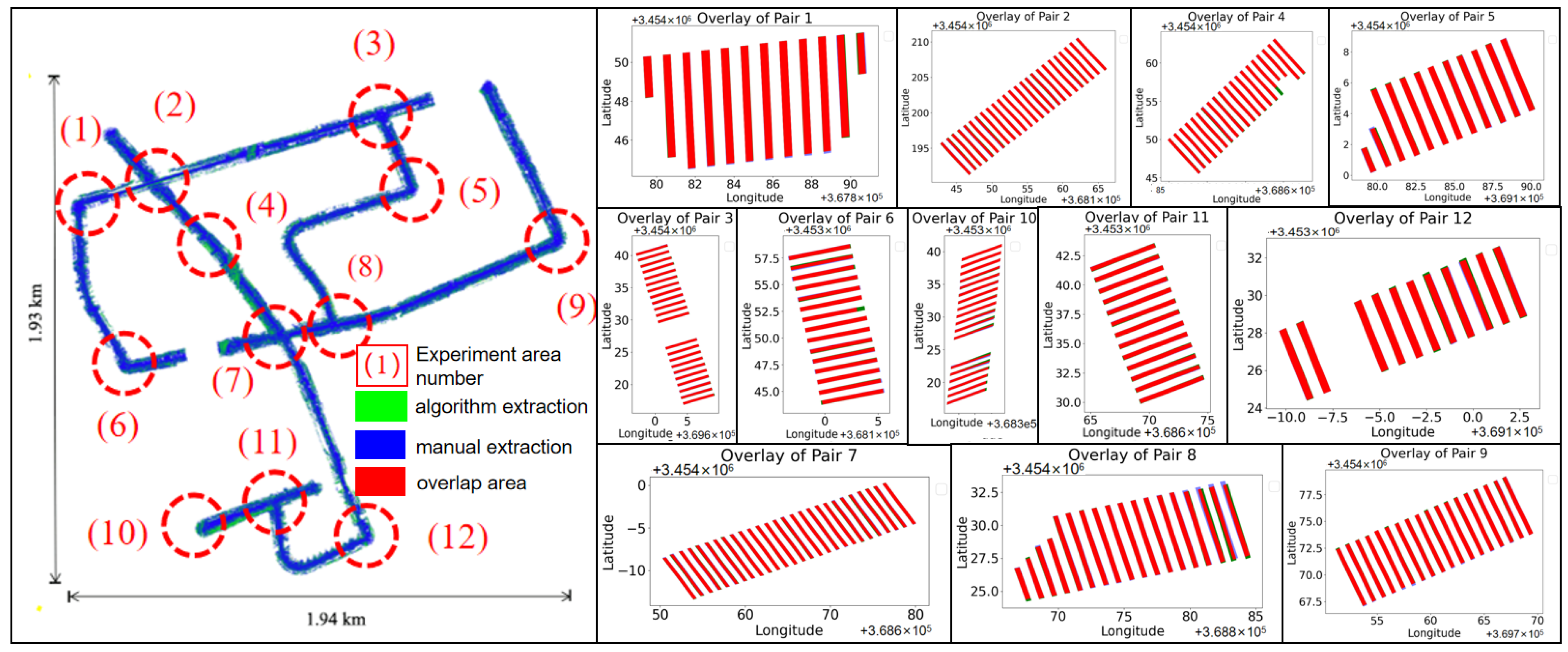
Point cloud data from eight roads in Shanghai were selected as the experimental subjects. These point clouds were extracted from the annotated WHU-Urban3D dataset [53] to facilitate accuracy comparison. This dataset encompasses various data types, including ALS point clouds, MLS point clouds, and panoramic images, all of which have undergone coordinate unification and registration. Specifically, the MLS data span over 6.5 × 10 3 m and includes additional attribute information such as intensity and number of returns, providing over 600 million per-point semantic and instance labels. The specific dataset utilized in this article is the Shanghai portion of the MLS-S dataset, obtained from the AS-900HL multi-platform LiDAR measurement system. The MLS-S dataset comprises 12 representative zebra crossing areas. The data distribution is illustrated in Figure 2, and the system’s specific parameters are listed in Table 1. Additionally, to further verify the robustness of the algorithm, we also conducted experiments using MLS point clouds obtained from other data acquisition platforms in Wuhan and Chengdu.

3.2. Research Framework

To meet the requirements for accuracy and precision in practical applications and to reduce the interference of outliers and other noise, we performed denoising and filtering preprocessing on all point cloud data using mainstream commercial software before commencing our work. When processing zebra crossings, we first manually marked the initial Regions of Interest (RoIs) through human–computer interaction. We then determined the number of zebra stripes by calculating the neighborhood intensity. Subsequently, we adaptively calculated the length of each zebra stripe and obtained its approximate location. Finally, we established a polygon template for each zebra stripe and constructed an energy function based on the intensity characteristics of the zebra crossings. This function was solved using the branch-and-bound method [54] and a multi-level solution space optimization strategy to determine the precise location and orientation of the zebra crossings, resulting in a three-dimensional reconstruction of the zebra crossings. The specific workflow is illustrated in Figure 3, and the algorithm was primarily implemented using C++ programming.

3.3. Zebra Stripe Count Calculation

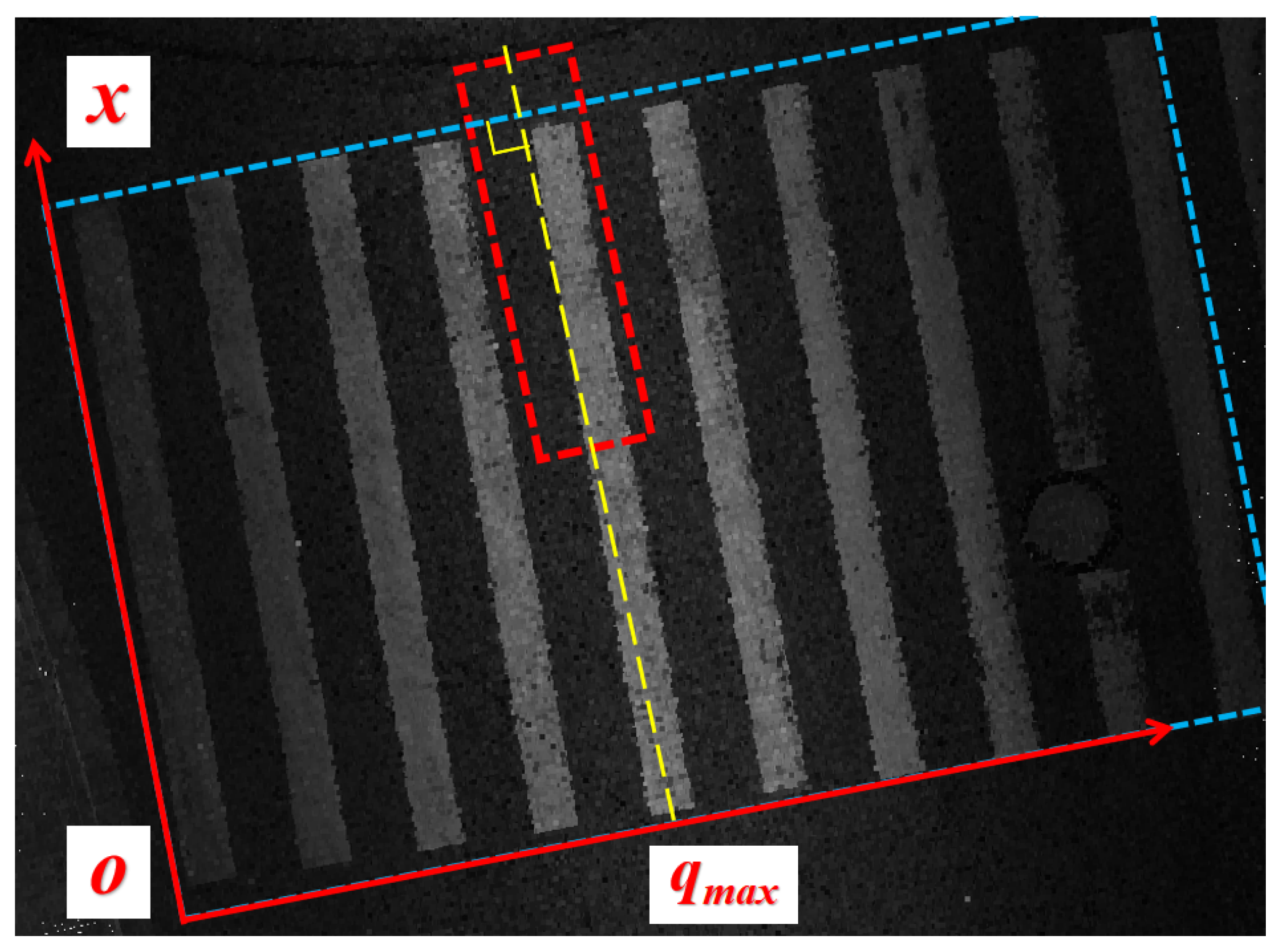
For ease of calculation and representation, we defined the direction along the long side of the zebra stripe within the pre-selection box as the x-axis, and the direction perpendicular to the x-axis as the y-axis. The z-axis aligns with the original coordinate system z-axis of the point cloud. Subsequently, we established a local coordinate system (as shown in Figure 4a). Within this local coordinate system, segmentation was performed at predetermined intervals along the y-axis. This resulted in the formation of the initial candidate coordinate point set, denoted as Q, which consists of points q i on the coordinate axis at each segmentation point. The energy E q of each q i was calculated, where E q is positively correlated with the reflection intensity of the nearby point cloud around q i . This energy represents the likelihood of q i being located near the central axis of the zebra stripe (Formulas (1) and (2)). From the candidate point set Q, the point q m a x with the maximum energy value, which is most likely to be near the centerline of the zebra crossing (as shown in Figure 4b), was continuously selected. Each selected point q m a x was recorded in the set Q m a x . According to the principle of non-maximum suppression, the selected point q m a x and its neighboring candidate points were automatically removed from the candidate point set Q (as shown in Formula (3)), until no candidate points remained in Q. At this point, the number of points in Q m a x corresponds to the number of zebra stripes in the selected area. Each candidate point position in Q m a x serves as the initial position of each zebra stripe on the y-axis. At these positions, fixed-size regions are defined above and below along the y-axis direction. These regions represent independent areas that contain a single stripe of the zebra crossing.
The energy E q is calculated for each candidate point as follows:
q n e a r = p | p . y q . y < w z e b r a / 2 , p C
E q = A q n e a r
where q n e a r represents the set of points near the candidate point q, p . y denotes the y-coordinate of point p, and q . y represents the y-coordinate of point q. The symbol | · | indicates taking the absolute value. The variable w z e b r a is the preset width of the zebra stripe (set to 0.45 m according to national standards in this paper). C represents the set of points within the pre-marked zebra crossing area, p is a point in the point set C, and q is a point in the candidate point set Q; A ( ) denotes the average reflection intensity of a point set; and E q refers to the average intensity of the point cloud within a width range of w z e b r a along the y-axis at point q.
Automatically iterate to update the candidate point set Q to q N e w according to the following formula:
q N e w = { q | | q . y q m a x . y | > K , q Q }
where q N e w represents the set of candidate points updated after each iteration, q m a x . y denotes the y-coordinate value of the central axis of the zebra stripe (approximately parallel to the x-axis) in the local coordinate system, and y = q m a x . y represents the equation of this axis in the local coordinate system. The threshold value K is determined within the range of [ w i n v / 2 , w i n v ], where w i n v is the interval between two parallel central axes of the zebra stripes (Figure 4b). It should be noted that if K is less than w i n v / 2 , the set Q m a x will include candidate points located between the two adjacent crossing stripe axes. On the other hand, if K is greater than w i n v , Q m a x may not include all the points near the zebra stripe axis. The specific value of K needs to be determined based on the experimental results.

3.4. Rough Pose Positioning

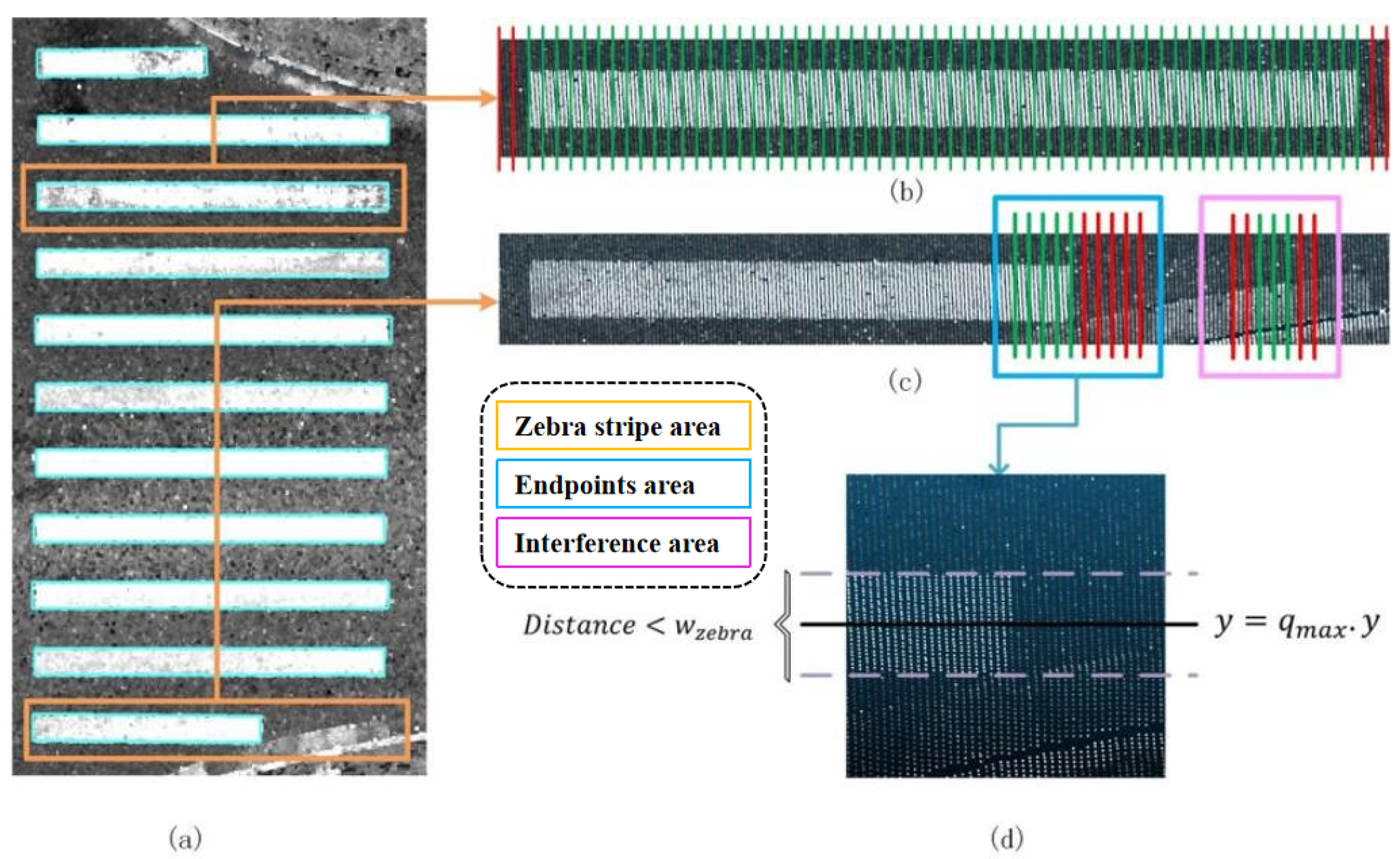
Based on Q m a x and the width w z e b r a of a single zebra stripe, independent areas containing a single zebra stripe can be determined; due to the high reflection intensity of zebra crossing point clouds, N candidate regions can be divided along the central axis direction at corresponding preset intervals. If there is a significant difference in intensity between point clouds near and far from the central axis, it is considered that this candidate region is located inside the zebra crossing. The length of each independent region’s zebra stripe is adaptively calculated and the rough position of the zebra crossing is obtained (as shown in Figure 5).
The determination of the candidate area for a zebra stripe is governed by the subsequent mathematical formula:
E j = A ( c | c . y c m a x . y | < w z e b r a / 2 , c J j ) A ( c | c . y c m a x . y | w z e b r a / 2 , c J j )
J j = b | b . x X m i n Δ t = j , b c m a x a r e a
c m a x a r e a = { p p . y c m a x . y < w z e b r a , p C }
where A ( ) represents the average intensity of the point set, and w z e b r a represents the width of a single zebra stripe. The symbol c m a x a r e a denotes the point set within an independent region that contains a single zebra stripe, c represents a point belonging to the set J j ( j = 1 , 2 , , N ) , J j represents the set of points in c m a x a r e a that fall within the candidate region, c m a x is the point corresponding to the region in the candidate point set Q m a x , c . y is the y-coordinate of the point c, and c m a x . y is the y-coordinate of the point c m a x . The symbol · represents an upward rounding operation, and Δ t represents the preset interval along the axis direction of the independent area of a single zebra stripe; C represents the set of points within the pre-selected overall zebra crossing area, and p represents a point in this set, b represents a point in the point set c m a x a r e a , b . x denotes the x-coordinate of point b, X m i n represents the minimum x-coordinate value of the point in the point set c m a x a r e a , and E j represents the intensity ratio of the points near the central axis of candidate region J j to the points away from the central axis. If E j > T z , it is considered that J j may be a zebra crossing area, which corresponds to the longer vertical area marked in Figure 5b,c.
We applied outlier filtering to the candidate regions that have the potential to be zebra crossings. Specifically, when a minimum of T L consecutive candidate regions are identified as possible zebra crossing regions, they are deemed to be correct zebra crossing regions. All these candidate regions, which are determined to be correct zebra crossings, constitute the set Q Z e b r a . For the zebra crossing template, we denote the length as L z e b r a . Additionally, we determine the initial center position of the template as P z e b r a .
L z e b r a = a r g m a x { r . x | r Q Z e b r a } a r g m i n { r . x | r Q Z e b r a }
P z e b r a . x = a r g m i n { r . x | r Q Z e b r a } + a r g m a x { r . x | r Q Z e b r a } 2
P z e b r a . y = c m a x . y
where a r g m a x { } is taken as the maximum value, and a r g m i n { } is taken as the minimum value; r represents a point from the set Q Z e b r a , and r . x specifically refers to the x-coordinate of point r; and P z e b r a . x represents the x-coordinate of the point P z e b r a , and P z e b r a . y represents the y-coordinate of point P z e b r a .

3.5. Template Matching and 3D Reconstruction

3.5.1. Energy Function Construction

According to national standards, zebra crossings have a fixed width and are predominantly rectangular in shape. Once the length of a zebra crossing is determined, a rectangular template can be constructed for each zebra crossing. However, variations in road intersection shapes can result in zebra crossings that are parallelograms. Hence, during template construction, the decision to deform the template can be made based on the pre-selection situation. For zebra crossings with parallelogram shapes, the angle between the template should match the angle between the two adjacent boundaries in the pre-selection area (e.g., the angle between boundary AO and boundary OB in Figure 4a). The template vertex consists of four ordered nodes, and the precise position of the zebra crossing can be represented by its center point position P ( x , y , z ) and its angle θ with respect to the x-axis of the global point cloud coordinate system.
There are differences in the laser reflection characteristics between the paint used for road traffic signs and the asphalt used on the road surface. In road scene point clouds, the intensity of the point cloud representing traffic signs is typically higher compared to the surrounding road surface. Based on this characteristic, a matching energy function E ( P , θ ) can be constructed, which includes the average intensity of the template-covered point cloud, intensity information entropy, and intensity gradient at the template boundary.
E ( P , θ ) = α · ϕ [ A I ] β · ϕ [ E I ] + γ · ϕ [ G I ]
E I = i = 0 i = m ( p i . I A I ) 2 m
G ( p ) = i = 0 i = k Δ I ( p , p i ) × sin ( p p i , L ) i = 0 i = k sin ( p p i , L )
where P represents the three-dimensional coordinates of the center point of the zebra crossing, and θ represents the angle between the long side direction of the zebra crossing and the x-axis of the overall point cloud coordinate system; A I represents the average intensity of the point cloud covered by a polygon template composed of four ordered nodes of a zebra crossing, E I represents the intensity information entropy of the point cloud covered by the zebra crossing, and G I represents the average intensity gradient of the point cloud at the boundary of the zebra crossing template; ϕ [ · ] represents Max-Min standardization; α , β , and γ are weight coefficients used to control the degree of influence of each item on the energy function; m is the number of point clouds covered by the template, and p i is the points covered by the template; p i . I represents the reflection intensity of point p i . G ( p ) represents the intensity gradient of point p in the direction perpendicular to the boundary of the zebra crossing template; Δ I ( p , p i ) represents the difference in intensity between point p and point p i ; p p i is the vector formed by connecting point p and point p i , as shown in the blue vector in Figure 6; L represents a vector composed of two ordered nodes connected near point p, as shown in the black vector in Figure 6. Due to the determined direction L of each edge in the template, this paper calculates the intensity gradient G ( p ) perpendicular to the template boundary, as shown in the purple vector in Figure 6, to weaken the influence of noise points on the intensity gradient calculation.
When the template accurately covers the zebra crossing point cloud, we can observe higher average intensity and smaller intensity information entropy. Additionally, the point cloud at the boundary exhibits a higher intensity gradient, resulting in a larger value for the energy function. Conversely, when the template only partially covers the point cloud representing the traffic sign, the average intensity is lower and the intensity information entropy is higher. This is due to the inclusion of a significant number of low-intensity ground points. Moreover, the intensity gradient at the boundary approaches zero, leading to a smaller value for the energy function.

3.5.2. Energy Function Solving

Solving energy functions can be categorized into two parts: solving continuous variables and solving discrete variables. The issue related to discrete variables is referred to as a combinatorial problem. Specifically, finding the optimal solution that satisfies the energy function from a limited number of discrete feasible solutions is known as a combinatorial optimization problem.
We utilized the RANSAC algorithm to fit the filtered ground point cloud and obtain the road plane equation. By combining the two-dimensional coordinates ( x , y ) of ordered nodes in the template with the plane equation, their three-dimensional spatial coordinates ( x , y , z ) can be obtained. Consequently, the four-dimensional solution space ( x , y , z , θ ) of the energy function can be simplified to a three-dimensional solution space ( x , y , θ ) . By searching for the optimal solution of the energy function E ( P , θ ) within the three-dimensional solution space ( x , y , θ ) , we can determine the precise position and direction information of the zebra crossing. This study models the process of seeking the optimal solution to the energy equation E ( P , θ ) as a combinatorial optimization problem, and draws inspiration from the idea of branch and bound [54] to quickly calculate its optimal solution. Firstly, a search tree is established, where each node represents a feasible solution s i in the solution space and corresponds to an energy function value s i . E ; then, the initial position and direction of the zebra crossing template are calculated using the coordinates of the three vertices of the initial rectangle RoI, serving as the root node of the search tree; finally, the child nodes of each node are taken as its adjacent (26-neighborhood) nodes in the solution space. The specific steps are as follows:
  • Calculate the energy function value of the root node, which represents the initial position and direction of the zebra crossing template determined by the coordinates of the three vertices of the initial rectangle RoI. This energy value is denoted as E m a x .
  • For all leaf nodes (when there is only one root node in the tree, the root node is considered a leaf node), calculate the solution set S N consisting of N feasible solutions in the 26-neighborhood of the corresponding solution space. Add the node corresponding to the solution set of { s | s . E > E max , s S N } to the search tree to become a new leaf node and update the E max = argmax { s . E | s S N } .
  • Repeat the previous step until no new leaf nodes are added to the search tree or the set iteration threshold is reached. At this stage, the feasible solution corresponding to E m a x represents the optimal solution, and the matching process is completed.

3.5.3. Local Coordinate System Update and Reconstruction Result Optimization

In the pre-selected RoIs for the zebra crossing, the number and length of the stripes vary significantly, making it challenging to accurately reconstruct them using fixed-size templates; therefore, they require computation. In extreme cases where there are fewer stripes, we initially set up the local coordinate system by aligning the X-axis along the long edge of a single stripe within the RoI, instead of the conventional method of aligning it along the short edge of the bounding box. This adjustment ensures the proper execution of the algorithm. However, this method still leads to issues such as errors in length measurement and a high computational load for template matching due to deviations in the initially selected x-axis from the actual conditions (as depicted in Figure 7). To address these challenges, after completing the first zebra crossing template matching, the matched zebra crossing direction was utilized as the new local coordinate system’s X-axis; the local coordinate system was then updated, and the energy value of the candidate point set Q was recalculated. In the updated local coordinate system, a continuous search was performed to find the candidate point q m a x that corresponded to the maximum energy value for template matching. Subsequently, the candidate point set was updated according to Formula (3) until there were no more candidate points in Q. This process enables the instance segmentation and preliminary 3D reconstruction of the zebra crossing area to be completed.
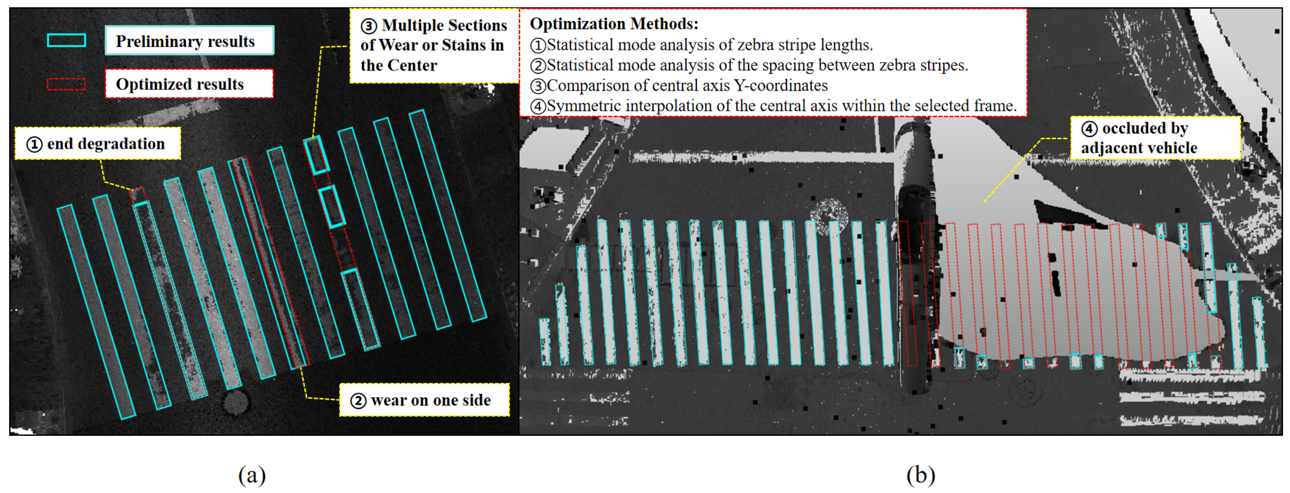
After the preliminary completion of regional reconstruction, the following four aspects were optimized and then the final zebra crossing area was constructed.
  • Zebra crossings with stained or damaged endpoints. This type of zebra crossing can lead to matching results that are shorter than the actual length. To address this issue, we analyzed the length characteristics of each stripe of the zebra crossing. For stripes located in the middle of the zebra crossing area or those with minimal length differences between them, we employed a method of “mode statistics and deformation metrics (stripe length and spacing) enforcement” to optimize the reconstruction results.
  • Zebra stripes with stains or damage in the middle. This type of zebra crossing can cause a zebra strip to be matched into two or even more segments. In this case, the y-coordinate of the axis in each matching result can be utilized to determine the completion of the splicing and fusion of the same zebra stripe.
  • Zebra stripes with unilateral damage. These defects can cause the extracted central axis, calculated using intensity measurements, to deviate to the left or right. To address this issue, after extracting all zebra stripe bands, we used the method of “mode statistics” to calculate the spacing between the stripes. We then adjusted the spacings that were close to the modal value to achieve uniform and optimized results.
  • Zebra stripes that are largely or completely obscured. This type of zebra crossing can lead to large blank areas in the matching results. To address this issue, our algorithm employs an axisymmetric interpolation technique to fill in the undetected zebra crossings within the zebra crossing area.

4. Results

To achieve superior extraction and reconstruction results, our algorithm has been carefully designed with distinct parameters at different stages. By incorporating the characteristics of the point cloud and the geometric features of zebra crossings, repeated experiments were conducted to determine the optimal settings. During the stage of identifying the number of zebra stripes, the preset interval Q t for the initial candidate point set Q was set to 5 cm, with the iterative filtering parameter K defined as 0.75 w i n v . When determining the length of the zebra stripe, the division interval Δ t was set to 5 cm, with a threshold T Z of 1.3 for the intensity ratio between points near and far from the central axis of a single zebra stripe. Additionally, the outlier filtering parameter T L was set to 5. During the template-matching stage, the weight parameters of the energy function were set to α = 1 , β = 1 , and γ = 2 in order to enhance the influence of zebra crossing boundaries on the energy function and obtain more accurate matching results. The specific parameter values are presented in Table 2.
Using the parameters determined from the aforementioned experiments, the proposed algorithm can effectively extract and reconstruct zebra crossings that exhibit various atypical characteristics, such as having a low number of zebra stripes, irregular lengths, or parallelogram shapes. The results of this process are illustrated in Figure 8.
Statistical analysis reveals that the 3D reconstruction time for each zebra crossing area is less than 1 s. From 12 representative zebra crossing areas selected for the experiments, one region containing several zebra stripes was randomly chosen from each as a comparison area, where the actual boundaries of each stripe were manually annotated. The degree of overlap between the algorithmic extraction results and the manual annotations for these 12 comparison areas is illustrated in Figure 9. Each zebra stripe reconstructed by the algorithm is bounded by four sequentially ordered vertices. For each stripe, the planar distance and elevation difference at the vertex i ( i = 1 , 2 , 3 , 4 ) are denoted as d i and e i , respectively. The average differences between these vertex indices are expressed as d i ¯ / e i ¯ ; the overall means for a single comparison area, D ¯ / E ¯ , Intersection over Union (IOU), precision, recall, and F1 score, along with the total average value M ¯ across all comparison areas, were used to evaluate the accuracy of the algorithm (where precision, recall, and the F1 score are calculated based on the number of point clouds encompassed by the zebra stripes). The results are presented in Table 3. It can be seen that the overall IoU for the sampled zones reaches 0.89, with the maximum error in average corner point plane positions being within 0.07 m and most errors within 0.05 m. Since the algorithm primarily extracts points from zebra crossings or nearby ground areas, the average error in corner point elevation is relatively small, approximately 0.01 m.
For the MLS point clouds obtained from other data acquisition platforms in Wuhan and Chengdu, the experimental results are shown in Figure 10. The statistical results, including the mean Intersection over Union (mIoU), mean planar Error of Position (mEoP), Distance Root Mean Square error (DRMS), precision, recall, and F1 score, are presented in Table 4. The precision and recall are calculated based on the number of point clouds enclosed by zebra stripe boundaries. It should be noted that the data in the table exclude zebra stripes with significant bias due to forced normalization. The overall IoU in the Shanghai experimental area reached 0.91, and the mEoP was within 0.05 m. The results indicate that the algorithm’s accuracy meets the requirements of practical production. Moreover, for areas with better point cloud quality, more pronounced reflectivity contrast, and fewer zebra crossing distortions (such as Wuhan), the extraction and reconstruction results are better.

5. Discussion

The algorithm utilized in this study employs a pre-selection RoI process facilitated by human–computer interaction. Since the selected area is typically small, it is not sensitive to point cloud density and reflectance intensity contrast, thereby bypassing the challenges associated with global multi-threshold settings and enabling adaptive computations. Additionally, it exhibits robustness in extracting zebra crossings, even in the presence of partial degradation, occlusion, and interference from other ground objects. Even severely occluded zebra crossings can benefit from satisfactory interpolation and symmetrical completion effects using this algorithm. For example, Figure 11a demonstrates a typical zebra crossing, featuring degradation and wear at the ends, multiple areas in the middle, and on one side. By utilizing mode statistics and comparing the y-coordinates of the central axis, our algorithm optimizes the reconstruction results, achieving a desirable level of accuracy. Similarly, in Figure 11b, a large blank area appears on the right side due to the parallel movement of other vehicles during scanning. To address this, the algorithm incorporates the concept of axial symmetry during the optimization phase, enabling the interpolation of the reconstruction results.
When solving the energy function, the approach involves first identifying the rough position and direction of the zebra crossing within a large margin { 5 , 0.10 m, 0.10 m} in the solution space. Subsequently, the spacing is gradually reduced to { 2 , 0.05 m, 0.05 m}, { 1 , 0.02 m, 0.02 m}, and { 0.5 , 0.01 m, 0.01 m}, enabling the calculation of the precise position and direction of the zebra crossing. This technique significantly reduces the computational load of the energy function compared to directly matching with the accuracy of { 0.5 , 0.01 m, 0.01 m}. When calculating energy functions with lower precision { 5 , 0.10 m, 0.10 m}, { 2 , 0.05 m, 0.05 m}, and {1°, 0.02 m, 0.02 m}, downsampling the MLS point cloud with a resolution of 0.05 m is performed to reduce data computation. To address the high time complexity associated with neighborhood search, which is a crucial step in calculating intensity gradients, a modification is made when computing the energy function with lower accuracy. It is observed that the intensity gradient at the boundary of the zebra crossing template is essentially 0 before high-precision matching at the interval { 0.5 , 0.01 m, 0.01 m}. Hence, when calculating the energy function with lower accuracy, only the average intensity term and intensity information entropy term are considered, while the intensity gradient term is disregarded. This approach not only ensures the accuracy of 3D reconstruction, but also effectively reduces the number of energy function calculations and improves algorithm efficiency.
For regions with significant positional errors and lower IoU values, our analysis reveals that these issues primarily result from severe wear near certain zebra crossing corners, unconventional painting methods, and systematic errors during some on-site painting processes. The manual extraction results were consistent with the actual scene, whereas the algorithm applied a post-processing optimization called “mode statistics and deformation metrics enforcement” during the extraction and reconstruction process. Although this optimization ensured consistency in the main lengths and intervals of the zebra stripes in the reconstruction, leading to standardized results, it could also lead to deviations from certain non-standard markings in the actual scene. As depicted in Figure 12a, to address low contrast in liDAR point cloud reflectivity due to infrequently updated paint, the algorithm typically selects zebra stripes with higher reflectivity as references. Despite a gradual increase in the length of the zebra stripe on the right side during painting, which did not exceed the threshold limits, the optimized result equalized the lengths of all zebra stripes in the middle, without affecting the extraction of noticeably shorter stripes on the far right. In Figure 12b, a middle zebra stripe was deliberately painted, excluding a manhole cover, the optimized extraction results ensured uniformity in length, and ideal reconstruction effects were still achieved in vehicle-obstructed blank areas. Figure 12c shows special slanted painting treatments on the zebra stripes on both sides of a central green median, with one stripe end severely worn, where the optimization ensured consistent extraction results. For such exceptional cases, decisions regarding adjustments should be based on the specific requirements of high-definition map construction.
While the algorithm presented in this paper offers several advantages, there are two notable limitations that warrant further research. First, the extraction results are suboptimal when cement cover slabs or white warning paint on the outer side of central green medians are in close proximity to zebra stripes, due to the similarity in reflectivity, as illustrated in Figure 13a. Second, for the outer areas far from the scanning trajectory line, due to the sparsity of the point clouds and the weakened contrast in reflectivity, the extraction performance is relatively poor, as shown in Figure 13b.
Additionally, it should be noted that the algorithm in this paper is specifically designed for point clouds acquired through MLS. We did not conduct comparative studies on point clouds obtained via non-vehicle methods like Terrestrial Laser Scanning (TLS) and Airborne Laser Scanning (ALS) due to differences in point cloud density and intensity contrast.

6. Conclusions

This paper adopts a direct processing approach for point clouds based on intensity information and the morphological characteristics of zebra crossings. This avoids the accuracy loss caused by converting point clouds into images and reduces the computational power and time pressure associated with boundary fitting algorithms. The RoI pre-selected by the human–machine interaction method avoids issues associated with the large-scale uneven distribution of intensity and normalization of intensity. Based on the acquisition of the numbers and lengths of zebra stripes, we select a quadrilateral template. Subsequently, an energy function is constructed, comprising the average intensity of the point cloud covered by the template, the entropy of the point cloud’s intensity information, and the intensity gradient at the template’s boundary. Solving this energy function facilitates the determination of the template’s best matching posture, which is crucial for completing the 3D reconstruction of the zebra stripes. Additionally, we optimize the reconstruction results for cases involving degradation or occlusion on the zebra stripes. During the resolution phase of the energy function, we implement strategies such as branch and bound and multi-scale solution space optimization. These strategies significantly reduce the computations required for the energy function, thereby improving the algorithm’s efficiency.
The experimental results demonstrate that the method proposed in this paper offers several advantages. It requires fewer manual interventions, exhibits a higher degree of automation, and is less affected by the surrounding terrain. The reconstruction speed is faster, and the accuracy is higher compared to other methods. Moreover, the proposed method showcases robustness in handling uneven distributions of point cloud density and intensity. It can also produce satisfactory results in areas with sparse point clouds and severe wear on zebra crossings.
The method we proposed demonstrates significant potential in various practical applications. Within intelligent transportation systems, it can enhance traffic management and pedestrian safety by accurately and promptly updating the positions and status of zebra crossings. For autonomous driving, integrating these precise 3D reconstructions into high-definition maps can improve vehicle localization and path planning, contributing to safer and more efficient navigation. Additionally, the ability to perform periodic rapid detection and reconstruction ensures that digital maps remain current, thus maintaining the reliability and accuracy of autonomous navigation systems.
In current applications, the LiDAR point clouds acquired generally include color attribute information, which future research can take into account. By using histograms of point cloud color distribution under local coordinate systems, it is possible to determine the width of individual zebra stripes and the spacing between them, further reducing the need for preset parameters. Moreover, the detection and reconstruction of roadside parking spaces, also painted with paint, can be explored using this algorithm in future steps.

Author Contributions

Conceptualization, Z.Z. and C.L.; methodology, Z.Z.; software, C.L.; validation, B.X., X.W. and S.G.; formal analysis, C.L. and S.G.; investigation, Z.Z. and B.X.; resources, C.L.; data curation, C.L.; writing—original draft preparation, Z.Z.; writing—review and editing, C.L., S.G. and X.W.; visualization, B.X.; supervision, S.G.; project administration, S.G.; funding acquisition, Z.Z. All authors have read and agreed to the published version of the manuscript.

Funding

This research was funded in part by the Yunnan Provincial Department of Education Science Research Fund Project, grant number 2023J1556. We would like to thank the anonymous reviewers and the editors.

Data Availability Statement

The related semantic instance dataset of point clouds in large-scale urban scenes (WHU-Urban3D) used in this article has been made publicly available at https://whu3d.com/ (accessed on 15 March 2024).

Acknowledgments

We appreciate Yang ’s research group for providing the real dataset used in this work; we also sincerely appreciate the valuable guidance, technical support, and data sharing support from the P2M software V3.0 development team.

Conflicts of Interest

The authors declare no conflicts of interest. The funders had no role in the design of this study; in the collection, analyses, or interpretation of data; in the writing of the manuscript; or in the decision to publish the results.

References

  1. Li, D.; Yao, Y.; Shao, Z. Big data in smart city. Geomat. Inf. Sci. Wuhan Univ. 2014, 39, 631–640. [Google Scholar]
  2. Wan, R.; Huang, Y.; Xie, R.; Ma, P. Combined lane mapping using a mobile mapping system. Remote Sens. 2019, 11, 305. [Google Scholar] [CrossRef]
  3. Ahilal, A.; Braud, T.; Lee, L.H.; Chen, H.; Hui, P. Toward A Traffic Metaverse with Shared Vehicle Perception. IEEE Commun. Stand. Mag. 2023, 7, 40–47. [Google Scholar] [CrossRef]
  4. Lehtomäki, M. Detection and Recognition of Objects from Mobile Laser Scanning Point Clouds: Case Studies in a Road Environment and Power Line Corridor; Aalto University: Espoo, Finland, 2021. [Google Scholar]
  5. Herumurti, D.; Uchimura, K.; Koutaki, G.; Uemura, T. Urban road network extraction based on zebra crossing detection from a very high resolution rgb aerial image and dsm data. In Proceedings of the 2013 International Conference on Signal-Image Technology & Internet-Based Systems, Kyoto, Japan, 2–5 December 2013; IEEE: New York, NY, USA, 2013; pp. 79–84. [Google Scholar]
  6. Koester, D.; Lunt, B.; Stiefelhagen, R. Zebra crossing detection from aerial imagery across countries. In Proceedings of the Computers Helping People with Special Needs: 15th International Conference, ICCHP 2016, Linz, Austria, 13–15 July 2016; Proceedings, Part II 15. Springer: Berlin, Germany, 2016; pp. 27–34. [Google Scholar]
  7. Yang, C.; Zhang, F.; Wang, J.; Huang, X.; Gao, Y. Extraction and reconstruction of zebra crossings from high resolution aerial images. Geomat. Inf. Sci. Wuhan Univ. 2017, 42, 1358–1364,1380. [Google Scholar]
  8. Zhong, J.; Feng, W.; Lei, Q.; Le, S.; Wei, X.; Wang, Y.; Wang, W. Improved U-net for zebra-crossing image segmentation. In Proceedings of the 2020 IEEE 6th International Conference on Computer and Communications (ICCC), Chengdu, China, 11–14 December 2020; IEEE: New York, NY, USA, 2020; pp. 388–393. [Google Scholar]
  9. Wang, H.; Sun, K.; Wang, Y. Zebra crossing segmentation based on dilated convolutions. In Proceedings of the 2021 4th International Conference on Advanced Electronic Materials, Computers and Software Engineering (AEMCSE), Changsha, China, 26–28 March 2021; IEEE: New York, NY, USA, 2021; pp. 522–527. [Google Scholar]
  10. Riveiro, B.; González-Jorge, H.; Martínez-Sánchez, J.; Díaz-Vilariño, L.; Arias, P. Automatic detection of zebra crossings from mobile LiDAR data. Opt. Laser Technol. 2015, 70, 63–70. [Google Scholar] [CrossRef]
  11. Li, L.; Zhang, D.; Ying, S.; Li, Y. Recognition and reconstruction of zebra crossings on roads from mobile laser scanning data. ISPRS Int. J. Geo-Inf. 2016, 5, 125. [Google Scholar] [CrossRef]
  12. Yan, L.; Liu, H.; Tan, J.; Li, Z.; Xie, H.; Chen, C. Scan line based road marking extraction from mobile LiDAR point clouds. Sensors 2016, 16, 903. [Google Scholar] [CrossRef]
  13. Rogers, S.R.; Manning, I.; Livingstone, W. Comparing the spatial accuracy of digital surface models from four unoccupied aerial systems: Photogrammetry versus LiDAR. Remote Sens. 2020, 12, 2806. [Google Scholar] [CrossRef]
  14. Sichelschmidt, S.; Haselhoff, A.; Kummert, A.; Roehder, M.; Elias, B.; Berns, K. Pedestrian crossing detecting as a part of an urban pedestrian safety system. In Proceedings of the 2010 IEEE Intelligent Vehicles Symposium, La Jolla, CA, USA, 2010; IEEE: New York, NY, USA, 2010; pp. 840–844. [Google Scholar]
  15. Wang, Y.; Chen, Q.; Zhu, Q.; Liu, L.; Li, C.; Zheng, D. A survey of mobile laser scanning applications and key techniques over urban areas. Remote Sens. 2019, 11, 1540. [Google Scholar] [CrossRef]
  16. Bi, S.; Yuan, C.; Liu, C.; Cheng, J.; Wang, W.; Cai, Y. A survey of low-cost 3D laser scanning technology. Appl. Sci. 2021, 11, 3938. [Google Scholar] [CrossRef]
  17. Di Stefano, F.; Chiappini, S.; Gorreja, A.; Balestra, M.; Pierdicca, R. Mobile 3D scan LiDAR: A literature review. Geomat. Nat. Hazards Risk 2021, 12, 2387–2429. [Google Scholar] [CrossRef]
  18. Nurunnabi, A.A.M.; Teferle, F.N.; Lindenbergh, R.; Li, J.; Zlatanova, S. Robust Approach for Urban Road Surface Extraction Using Mobile Laser Scanning Data. In Proceedings of the ISPRS Congress, Nice, France, 6–11 June 2022. [Google Scholar]
  19. Li, F.; Zhou, Z.; Xiao, J.; Chen, R.; Lehtomäki, M.; Elberink, S.O.; Vosselman, G.; Hyyppä, J.; Chen, Y.; Kukko, A. Instance-aware semantic segmentation of road furniture in mobile laser scanning data. IEEE Trans. Intell. Transp. Syst. 2022, 23, 17516–17529. [Google Scholar] [CrossRef]
  20. Schneider, D.; Blaskow, R. Boat-based mobile laser scanning for shoreline monitoring of large lakes. Int. Arch. Photogramm. Remote Sens. Spat. Inf. Sci. 2021, 43, 759–762. [Google Scholar] [CrossRef]
  21. Vandendaele, B.; Martin-Ducup, O.; Fournier, R.A.; Pelletier, G. Evaluation of mobile laser scanning acquisition scenarios for automated wood volume estimation in a temperate hardwood forest using Quantitative Structural Models. Can. J. For. Res. 2024. [Google Scholar] [CrossRef]
  22. Huang, R.; Dong, M.; Luo, F.; Sun, P. Identification of graphical shapes based on vanishing point column. Comput. Eng. Des. 2018, 39, 1433–1438. [Google Scholar]
  23. Chen, P.R.; Lo, S.Y.; Hang, H.M.; Chan, S.W.; Lin, J.J. Efficient Road Lane Marking Detection with Deep Learning. arXiv 2018, arXiv:1809.03994. [Google Scholar]
  24. Pan, X.; Gao, L.; Marinoni, A.; Zhang, B.; Yang, F.; Gamba, P. Semantic labeling of high resolution aerial imagery and LiDAR data with fine segmentation network. Remote Sens. 2018, 10, 743. [Google Scholar] [CrossRef]
  25. Cheng, H.; Jiang, Z.; Cheng, K. Semantic segmentation of zebra crossing based on improved SegNet model. Electron. Meas. Technol. 2020, 43, 104–108. [Google Scholar]
  26. Wu, X.H.; Hu, R.; Bao, Y.Q. Block-based hough transform for recognition of zebra crossing in natural scene images. IEEE Access 2019, 7, 59895–59902. [Google Scholar] [CrossRef]
  27. Zhou, B.; Li, Z.; Li, Y.; Li, J. Treatment and recognition of zebra crossing under uneven illumination. Electron. Des. Eng. 2020, 28, 168–172. [Google Scholar]
  28. Chen, N.; Hong, F.; Bai, B. Zebra crossing recognition method based on edge feature and Hough transform. J. Zhejiang Univ. Sci. Technol. 2019, 31, 476–483. [Google Scholar]
  29. Wang, Y.; Xu, C. A zebra crossing recognition method based on improved inverse perspective mapping. J. North China Univ. Technol. 2013, 25, 31–35,66. [Google Scholar]
  30. Ahmed, A.; Ashfaque, M.; Ulhaq, M.U.; Mathavan, S.; Kamal, K.; Rahman, M. Pothole 3D reconstruction with a novel imaging system and structure from motion techniques. IEEE Trans. Intell. Transp. Syst. 2021, 23, 4685–4694. [Google Scholar] [CrossRef]
  31. Huang, S.; Liu, H.; Zhou, K.; Liu, J. Zebra crossing segmentation based on improved unet. Intell. Comput. Appl. 2020, 10, 61–64,69. [Google Scholar]
  32. Xu, X.; Dong, S.; Xu, T.; Ding, L.; Wang, J.; Jiang, P.; Song, L.; Li, J. Fusionrcnn: Lidar-camera fusion for two-stage 3d object detection. Remote Sens. 2023, 15, 1839. [Google Scholar] [CrossRef]
  33. Ma, D.; Wang, N.; Fang, H.; Chen, W.; Li, B.; Zhai, K. Attention-optimized 3D segmentation and reconstruction system for sewer pipelines employing multi-view images. Comput.-Aided Civil Infrastruct. Eng. 2024; early view. [Google Scholar]
  34. Wu, X.H.; Hu, R.; Bao, Y.Q. A regression approach to zebra crossing detection based on convolutional neural networks. IET Cyber-Syst. Robot. 2021, 3, 44–52. [Google Scholar] [CrossRef]
  35. Sinha, P.K.; Ghodmare, S.D. Zebra Crossing Detection and Time Scheduling Accuracy, Enhancement Optimization Using Artificial Intelligence. Int. J. Sci. Res. Sci. Technol. 2021, 8, 515–525. [Google Scholar] [CrossRef]
  36. Zhang, C.; Chen, X.; Liu, P.; He, B.; Li, W.; Song, T. Automated detection and segmentation of tunnel defects and objects using YOLOv8-CM. Tunn. Undergr. Space Technol. 2024, 150, 105857. [Google Scholar] [CrossRef]
  37. Williams, K.; Olsen, M.J.; Roe, G.V.; Glennie, C. Synthesis of transportation applications of mobile LiDAR. Remote Sens. 2013, 5, 4652–4692. [Google Scholar] [CrossRef]
  38. Gharineiat, Z.; Tarsha Kurdi, F.; Campbell, G. Review of automatic processing of topography and surface feature identification LiDAR data using machine learning techniques. Remote Sens. 2022, 14, 4685. [Google Scholar] [CrossRef]
  39. Gargoum, S.A.; El Basyouny, K. A literature synthesis of LiDAR applications in transportation: Feature extraction and geometric assessments of highways. GISci. Remote Sens. 2019, 56, 864–893. [Google Scholar] [CrossRef]
  40. Chang, L.; Niu, X.; Liu, T.; Tang, J.; Qian, C. GNSS/INS/LiDAR-SLAM integrated navigation system based on graph optimization. Remote Sens. 2019, 11, 1009. [Google Scholar] [CrossRef]
  41. Soilán, M.; Justo, A.; Sánchez-Rodríguez, A.; Riveiro, B. 3D point cloud to BIM: Semi-automated framework to define IFC alignment entities from MLS-acquired LiDAR data of highway roads. Remote Sens. 2020, 12, 2301. [Google Scholar] [CrossRef]
  42. Ma, L.; Li, Y.; Li, J.; Wang, C.; Wang, R.; Chapman, M.A. Mobile laser scanned point-clouds for road object detection and extraction: A review. Remote Sens. 2018, 10, 1531. [Google Scholar] [CrossRef]
  43. Yang, R.; Li, Q.; Tan, J.; Li, S.; Chen, X. Accurate road marking detection from noisy point clouds acquired by low-cost mobile LiDAR systems. ISPRS Int. J. Geo-Inf. 2020, 9, 608. [Google Scholar] [CrossRef]
  44. Zhu, E. An algorithm for extracting zebra line angle from Mobile Laser Scanner point clouds. Remote Sens. Inf. 2021, 36, 59–63. [Google Scholar]
  45. Yang, M.; Wan, Y.; Liu, X.; Xu, J.; Wei, Z.; Chen, M.; Sheng, P. Laser data based automatic recognition and maintenance of road markings from MLS system. Opt. Laser Technol. 2018, 107, 192–203. [Google Scholar] [CrossRef]
  46. Esmorís, A.M.; Vilariño, D.L.; Arango, D.F.; Varela-García, F.A.; Cabaleiro, J.C.; Rivera, F.F. Characterizing zebra crossing zones using LiDAR data. Comput.-Aided Civil Infrastruct. Eng. 2023, 38, 1767–1788. [Google Scholar] [CrossRef]
  47. Zhang, J.; Lin, X.; Ning, X. SVM-based classification of segmented airborne LiDAR point clouds in urban areas. Remote Sens. 2013, 5, 3749–3775. [Google Scholar] [CrossRef]
  48. Fang, L.; Huang, Z.; Luo, H.; Chen, C. Integrating SVM and graph matching for identifying road markings from mobile LiDAR point clouds. J. Geo-Inf. Sci. 2019, 21, 994–1008. [Google Scholar]
  49. Fang, L.; Wang, S.; Zhao, Z.; Fu, H.; Chen, C. Automatic classification and vectorization of road markings from mobile laser point clouds. Acta Geod. Cartogr. Sin. 2021, 50, 1251. [Google Scholar]
  50. Soilán, M.; Riveiro, B.; Martínez-Sánchez, J.; Arias, P. Segmentation and classification of road markings using MLS data. ISPRS J. Photogramm. Remote Sens. 2017, 123, 94–103. [Google Scholar] [CrossRef]
  51. Wen, C.; Sun, X.; Li, J.; Wang, C.; Guo, Y.; Habib, A. A deep learning framework for road marking extraction, classification and completion from mobile laser scanning point clouds. ISPRS J. Photogramm. Remote Sens. 2019, 147, 178–192. [Google Scholar] [CrossRef]
  52. Zeng, H.; Chen, Y.; Zhang, Z.; Wang, C.; Li, J. Reconstruction of 3D Zebra Crossings from Mobile Laser Scanning Point Clouds. In Proceedings of the IGARSS 2019—2019 IEEE International Geoscience and Remote Sensing Symposium, Yokohama, Japan, 28 July–2 August 2019; IEEE: New York, NY, USA, 2019; pp. 1899–1902. [Google Scholar]
  53. Han, X.; Liu, C.; Zhou, Y.; Tan, K.; Dong, Z.; Yang, B. WHU-Urban3D: An urban scene LiDAR point cloud dataset for semantic instance segmentation. ISPRS J. Photogramm. Remote Sens. 2024, 209, 500–513. [Google Scholar] [CrossRef]
  54. Lawler, E.L.; Wood, D.E. Branch-and-bound methods: A survey. Oper. Res. 1966, 14, 699–719. [Google Scholar] [CrossRef]
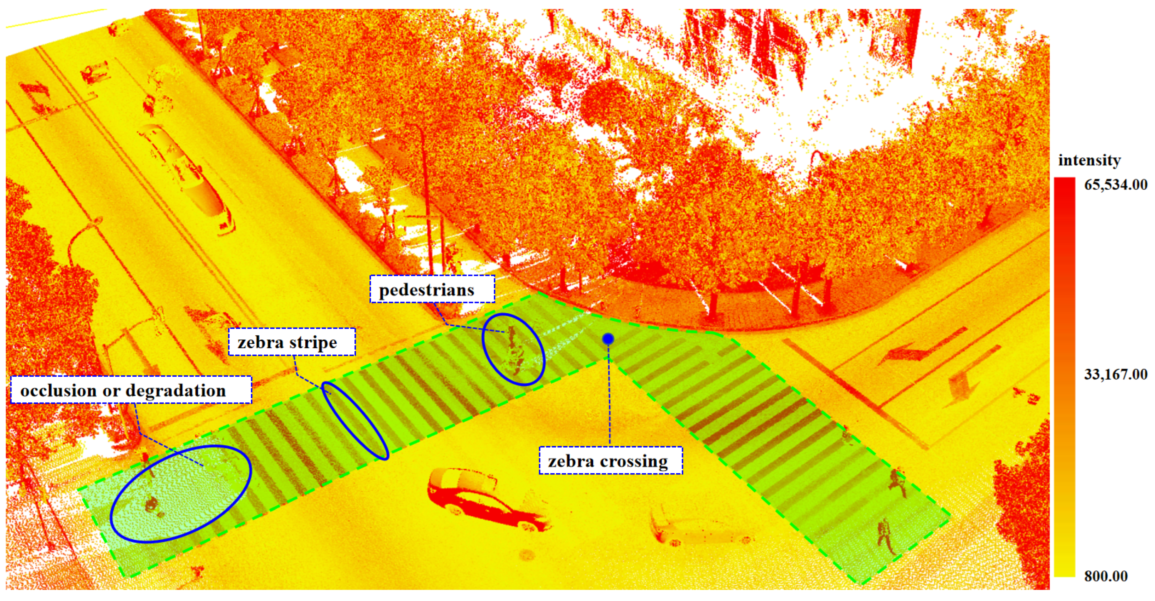
Figure 1. Zebra crossings in LiDAR point cloud represented by intensity.
Remotesensing 16 03722 g001
Figure 2. Study case. (a) AS-900HL multi-platform LiDAR measurement system. (b) Trajectory of the study case (Shanghai, China). (c) Distribution of zebra crossing areas used for experiments in the MLS-S point cloud.
Remotesensing 16 03722 g002
Figure 3. Overall workflow of zebra crossing extraction and 3D reconstruction.
Remotesensing 16 03722 g003
Figure 4. Calculation of stripe count in pre-selection box. (a) Local coordinate system of the selected zebra crossing area. (b) Candidate point q i and the point q m a x with the highest local energy value.
Remotesensing 16 03722 g004
Figure 5. Calculation of single zebra stripe length. (a) Typical zebra crossing; (b) Regular zebra stripes; (c) Zebra stripes at the curb; (d) Zoomed-in view.
Remotesensing 16 03722 g005
Figure 6. Schematic of template boundary intensity gradient calculation.
Remotesensing 16 03722 g006
Figure 7. Length calculation error caused by deviation of the pre-selected box.
Remotesensing 16 03722 g007
Figure 8. Extraction and reconstruction results of alienated zebra crossings. (a) Regular zebra crossing. (b) Zebra crossings with varying lengths or fewer stripes. (c) Parallelogram zebra crossing.
Remotesensing 16 03722 g008
Figure 9. IOUs of horizontal projections between algorithm results and manual annotations.
Remotesensing 16 03722 g009
Figure 10. Experimental results of MLS point clouds from Wuhan and Chengdu obtained by other data collection platforms.
Remotesensing 16 03722 g010
Figure 11. Extraction and reconstruction results of zebra crossings under interference conditions. (a) Partially stained zebra crossings. (b) Zebra stripes with partial point clouds missing due to occlusion.
Remotesensing 16 03722 g011
Figure 12. Accuracy reduction caused by endpoint contamination or systematic spraying errors. (a) Systematic painting minor errors. (b) Vehicle obstruction and manhole cover occupation. (c) Special cases.
Remotesensing 16 03722 g012
Figure 13. Limitations of the algorithm under special circumstances. (a) Limitation case 1. (b) Limitation case 2.
Remotesensing 16 03722 g013
Table 1. Parameters of the AS-900HL multi-platform LiDAR measurement system(Shanghai Huace Navigation Technology Ltd., Shanghai, China).
ParameterValue
Scanning frequency200 Hz
Laser emission frequency550 k pts/s
Panoramic camera resolution8192 × 4096
Maximum scanning distance920 m
Table 2. Descriptions and settings of vital parameters.
ParameterDescriptionValue
Q t The selection interval of the initial candidate point set Q 5 cm
K Iterative update filtering coefficient0.75 w inv
Δ t The division interval of a single zebra crossing5 cm
T Z The threshold for the ratio of single zebra crossing intensity to surrounding intensity1.3
T L Outlier filtering parameter5
α , β , γ The weight of the energy function1, 1, 2
Table 3. Accuracy of zebra crossing extraction and reconstruction.
Pair IDNumber of Zebra Stripes d 1 ¯ / e 1 ¯ (m) d 2 ¯ / e 2 ¯ (m) d 3 ¯ / e 3 ¯ (m) d 4 ¯ / e 4 ¯ (m) D ¯ / E ¯ (m)IOUPrecisionRecallF1 Score
1120.06/0.010.05/0.000.01/0.000.01/0.000.04/0.000.9497.7297.2497.48
2250.04/0.020.03/0.020.03/0.010.03/0.010.03/0.010.9094.6393.7294.17
3220.05/0.020.03/0.020.03/0.010.04/0.020.04/0.020.9297.0095.7196.35
11130.04/0.010.05/0.020.04/0.010.05/0.010.05/0.010.9194.3096.0295.15
12110.04/0.010.03/0.010.04/0.010.05/0.010.04/0.010.9194.9297.2496.06
M ¯ 17.60.07/0.010.05/0.010.04/0.010.05/0.010.05/0.010.8995.0495.1695.10
Table 4. Comparison of zebra crossing reconstruction results and manual annotation results.
Study AreaNumber of Zebra Crossing AreasTotal Number of Zebra StripesmIoUmEoP (cm)DRMS (cm)PrecisionRecallF1 Score
Shanghai122010.914.14.995.5995.3195.45
Wuhan81290.942.53.595.9497.2796.60
Chengdu71180.894.04.695.8692.5394.16
Disclaimer/Publisher’s Note: The statements, opinions and data contained in all publications are solely those of the individual author(s) and contributor(s) and not of MDPI and/or the editor(s). MDPI and/or the editor(s) disclaim responsibility for any injury to people or property resulting from any ideas, methods, instructions or products referred to in the content.