Abstract
Online maps are of great importance in modern life, especially in commuting, traveling and urban planning. The accessibility of remote sensing (RS) images has contributed to the widespread practice of generating online maps based on RS images. The previous works leverage an idea of domain mapping to achieve end-to-end remote sensing image-to-map translation (RSMT). Although existing methods are effective and efficient for online map generation, generated online maps still suffer from ground features distortion and boundary inaccuracy to a certain extent. Recently, the emergence of diffusion models has signaled a significant advance in high-fidelity image synthesis. Based on rigorous mathematical theories, denoising diffusion models can offer controllable generation in sampling process, which are very suitable for end-to-end RSMT. Therefore, we design a novel end-to-end diffusion model to generate online maps directly from remote sensing images, called MapGen-Diff. We leverage a strategy inspired by Brownian motion to make a trade-off between the diversity and the accuracy of generation process. Meanwhile, an image compression module is proposed to map the raw images into the latent space for capturing more perception features. In order to enhance the geometric accuracy of ground features, a consistency regularization is designed, which allows the model to generate maps with clearer boundaries and colorization. Compared to several state-of-the-art methods, the proposed MapGen-Diff achieves outstanding performance, especially a RMSE and SSIM improvement on Los Angeles and Toronto datasets. The visualization results also demonstrate more accurate local details and higher quality.
1. Introduction
The adaptability and economic viability of remote sensing images have led to their widespread adoption in the generation of online maps. The traditional map-generating method requires significant human involvement, which is laborious, extensive and time-consuming. In some emergency situations, such as earthquakes, the traditional method may not provide a timely map-generating and updating service [1]. Therefore, it is of great importance to propose a method to quickly generate accurate maps in emergency situations.
The application of deep learning has demonstrated considerable potential in the field of remote sensing image processing, such as object extraction, classification [2,3], automatic detection [4], road and building extraction [5,6,7] and semantic segmentation [8]. The fast development of deep learning generative modes in the image synthesis field provides a new alternative to online map generation. In the context of the generative framework, input images and target results are conceptualized as two distinct domains. The generative model attempts to use Generative Adversarial Networks (GANs) [9] as a domain mapping method to conduct translation between domains. The current GAN-based image translation model is originally from Conditional GANs (CGANs) [10], such as Pix2Pix [11] and CycleGAN [12]. Ganguli et al. present an innovative method for the translation of RS images-to-online maps [13]. However, the CycleGAN only proposes a cyclic consistency loss to control generation, which makes the results suffer from inaccurate details. Moreover, some other methods [14,15,16] perform more exploration for remote sensing image-to-map translation (RSMT). Nonetheless, these applications of general GANs to the domain of map translation exhibit several inherent limitations [17]. Figure 1 illustrates the unresolved problems in the existing works. To address these problems, Song et al. propose more loss functions to enhance model performance. For example, a geometric consistency is implemented in MapGen-GAN [18] to increase the accuracy of the translated maps compared with CycleGAN, which implies that, for specific tasks, some designed loss functions are vitally important. While previous works based on GANs achieved outstanding performance on most online map generation tasks, they still fall short in terms of capturing more diversity [19], particularly in terms of mode coverage, which may result in blurred boundaries and semantic distortion for the RSMT. Therefore, it is evident that the construction of a new model is required in order to address the challenge of more diversity elements in remote sensing images.
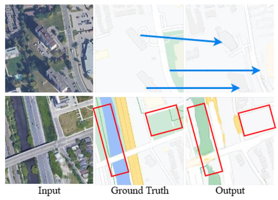
Figure 1.
The previous methods for the RSMT have faced some challenges in local detail inaccuracy and semantic distortion. The blue markers show the blurred boundaries of urban roads and buildings; the red rectangular box shows incorrect semantic colorization.
Diffusion Models (DMs) represent a category of likelihood-based models that have proven adept at generating high-fidelity images across various image processing tasks, while also providing beneficial characteristics such as comprehensive distribution coverage, a stable optimization target and straightforward scalability [20]. Therefore, DMs have more advantages in handling images with more diversity, such as remote sensing images. Moreover, DMs generate samples by gradually predicting future results from a Gaussian signal, and they consider reweighted variational lower bounds as the training objective, which have a more solid mathematic foundation than GAN-based methods. However, most of the conditional diffusion models have just been applied to natural images [21] instead of RSMT. Thus, more geometric loss functions are required to mitigate ground feature distortion and boundary inaccuracy phenomena in generated maps.
To this end, we explore the practicability of online map translation from RS images based on diffusion models. In order to achieve controllable generation and reduce randomness in sampling, we adopt a denoising diffusion bridge model to learn the distribution between RS images and online maps directly through the bidirectional diffusion process. For more abstract features and an enhancement of the visual perception in RS images, we implement a pretrained encoder [22] to map the images into a latent feature space. Moreover, transformation consistency regularization (TCR) loss is employed to enhance the geometric accuracy of the generated online maps. The principal methodology and major contribution of our study are presented below:
- 1.
- The diffusion model is introduced to the specific translation task between remote sensing images and online maps. To avoid the randomness of generated images, we propose an improved denoising diffusion bridge to establish a mapping between two domains. To the best of our knowledge, our work is the first RSMT exploration based on diffusion models.
- 2.
- To further improve the performance of the proposed model, we employ a pretrained encoder for image compression into the latent space, which may capture more features with diversity. Additionally, a transformation consistency regularization is proposed for more accurate geometric details.
- 3.
- Extensive experiments are conducted on two commonly used open datasets, Los Angeles and Toronto datasets, to validate the effectiveness and applicability of our methods. The experimental results demonstrate that MapGen-Diff can enhance the quality of generation, achieving significantly better performance than the previous translation methods.
The subsequent sections are organized as follows: Section 2 offers a comprehensive review on map translation methodologies and the application of diffusion models for image synthesis. In Section 3, we present the mechanism of the denoising diffusion bridge and the loss function. Then, the experiment results and an ablation study are shown in Section 4. In Section 5, we conduct some in-depth discussions of downsampling factor’s and sampling steps’ influence on the accuracy and diversity of the results. Finally, the conclusions and future directions are outlined in Section 6.
2. Related Work
In this section, we briefly illustrate the related work of image-to-image translation, DM-based image generation technology and the development of the DM mechanism.
2.1. Image-to-Image Translation
With the advent of deep learning, generative models have developed rapidly in the field of image processing. In particular, GANs have been extensively employed in the image translation task. One of typical methods of image translation is Pix2pix [11], which is a full supervised model based on the conditional GAN (CGAN) [10]. Since the Pix2pix employs one-to-one strictly matched samples, it is unstable and lacks diversity. The BicycleGAN proposes an idea of adding constrains to the bijective consistency of output and utilizing a latent coding layer [23]. Meanwhile, Ganguli et al. [13] proposed GeoGAN to this specific task by introducing reconstruction loss and style transfer loss as GAN loss. However, supervised learning needs accurately matched data, which are laborious.
The acquisition of well-matched samples represents a difficulty in practical applications. To handle this problem, some studies employ an unsupervised learning strategy. For example, Zhu [12] builds a network called CycleGAN, which proposes cycle consistency to make a model that works with unpaired data. DualGAN [24] and DiscoGAN [25] are also typical models used for image translation. To improve the generation quality under unpaired samples, the GcGAN proposed geometric consistency to establish a perfect mapping between two domains. Song et al. [18] design a robust unsupervised network framework to generate map tiles by using an improved U-Net based on previous works. While more loss functions are proposed to enhance the performance of the unsupervised model, unmatched data may result in mode collapse, which extremely influences the translation quality.
Moreover, a recent study has focused on a semi-supervised learning method, SMAPGAN [26], to address the topological consistency between pixel relationships in a synthesized map, employing an L1 norm and structural loss for image gradients to address the topological consistency between pixel relationships in a translated map. Semi-MapGen [27] proposed a teacher–student knowledge extensive network, which achieved outstanding results in a map generation task. However, GAN-based methods seems to be unstable as a result of the competitive process between the generator and discriminator.
Recently, with the popularity of the diffusion model, many advanced works have focused on applying diffusion models to image translation, such as conditional DMs [17]. Based on the work of [17], some works consider images from an origin domain as guidance in the sampling process [28,29,30]. Furthermore, Li et al. [21] introduced the ideas of the diffusion bridge to image translation, which has a fixed endpoint regarding the diffusion process and achieves competitive performance in natural image generation.
2.2. Diffusion Model
As a class of stochastic generative models, diffusion models initiate the process of data destruction by incrementally adding noise. Then, the generation of target images starts from learning to reverse this process [31]. There are three dominant models in the current general DMs: denoising diffusion probabilistic models (DDPMs) [20,32,33], score-based generative models (SGMs) [34,35] and stochastic differential equations (Score SDEs) [3,36].
Based on Markov chains, DDPMs achieve generation through a forward diffusion process and reverse denoising process. With a transition kernel , we can generate a sequence of random noise by providing initial data . The objective of the denoising process is to predict the original from pure noise based on the reverse chain.
The core process of the prediction is contingent upon the training of the reverse Markov chain to align with the actual time reversal of the forward Markov chain. This is accomplished by minimizing the Kullback–Leibler (KL) divergence, which means that the objective of the training process is to optimize the Evidence Lower Bound (ELBO). Within the case of infinite time steps or noise levels of DDPMs and SGMs, a new type of DM can be generalized as another formula, stochastic differential equations (SDEs).
However, the limitation of general diffusion models is that the reverse process starts from standard Gaussian distributions, which cannot naturally convert between two arbitrary distributions. Doob’s h-transform [37] introduces a method to solve a fixed endpoint situation. Therefore, the denoising diffusion bridge (DDBM) [38,39], which sets the condition , is proposed by [40].
2.3. Diffusion Model-Based Image Generation Technology
Recently, DMs have achieved impressive performances on natural image generation [17,30], inpainting [28], super-resolution [41] and text-to-image generation [42,43]. Ho et al. [20] were the first to create a denoising diffusion probabilistic model (DDPM), which pioneers a novel method of image processing and acquires more outstanding performance. However, the normal DDPM cannot control the result quality from random Gaussian noise based on a single diffusion process. The conditional diffusion model is proposed with a classifier, which is trained on ImageNet [17]. This network makes the diffusion model a novel alternative choice. Therefore, Palette [28] deployed the diffusion model in the field of colorization, inpainting, uncropping and JPEG restoration. Inspired by CycleGAN, Sasaki et al. [44] proposed the UNIT-DDPM based on Langevin dynamics, which generates target images with consistency constraints under the guidance of images from a source domain. Moreover, Wang et al. [29] provided a new network, PITI, based on a pretrained normal model. PITI regards each image translation task as a downstream task and utilizes a pretrained model to accommodate different types of translations, and it is also regarded as a generic framework to these tasks. Since that, the pretrained model and finetuned method have become a paradigm in various specific tasks.
However, the diffusion model is an auto-regressive model that requires a repeated iterative computation, which is computationally resource-intensive for training and inference. The latent diffusion model [22] proposed a pair of encoders and decoders to map pixel images into a latent space, which decreased the computation complexity. According to the works above, Stability AI provides a stable diffusion model, which becomes a generalized framework for pretraining in most image processing tasks.
Based on stable diffusion, Choi et al. [45] employed a pretrained stable diffusion model and controlled the reverse process to achieve high-quality generation under the guidance of a reference classifier. The SDEDIT [46] used the stochastic differential equation to guide the generation, outperforming previous GAN-based methods in realism and reliability. The EGSDE [47] also introduced two feature extractors to add reference image guidance. Moreover, Wu et al. [48] proposed cycle diffusion that was applied in unpaired image translation and zero-shot image editing. Sun et al. [49] presented a new score-decomposed diffusion model, which achieved best performance in natural images processing.
3. Methods
In this section, firstly, we illustrate the framework of the MapGen-Diff. Then, we present the details of image compression into the latent space, diffusion process and designed loss function separately.
3.1. Overall Architecture
We design an end-to-end denoising diffusion bridge network to conduct the RSMT. The main framework of our model is presented in Figure 2.
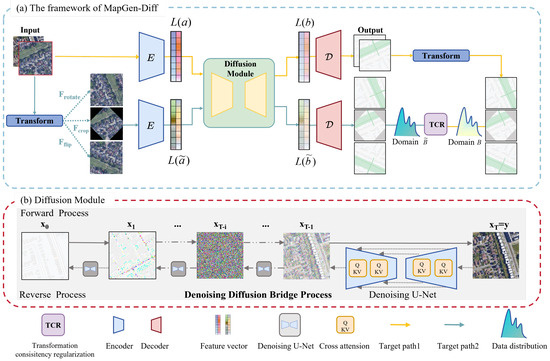
Figure 2.
Overall architecture of our proposed model MapGen-Diff. Part (a) illustrates the pipeline of MapGen-Diff. There are two diffusion processes with shared weights. First, we use an encoder E to map the remote sensing images from pixel space into feature space. Second, through the transformation function =, we train the network separately on original and transformed data. Finally, we adopt TCR loss to retain the consistency between original data and transformed data. Part (b) shows the detailed diffusion process. We utilize the data distribution from Domain A and Domain B as the endpoints of the diffusion process. While sampling in the reverse process, we utilize a U-Net network in the denoising process to control the generation in the feature space.
Given a paired data sampled from Domain A and Domain B, our task aims to learn the data mapping mechanism and implement the diffusion process between two domains. For more abstract features, we initiate the diffusion process by mapping the pixel space into the latent feature space and via a pretrained encoder E and decoder of Vector Quantization GAN (VQGAN) [50]. The is sampled from Domains and , which are obtained by applying . is a geometric transformation function that aims to illustrate regularization transformation, including rotation, flipping and cropping.
Our model includes two diffusion process: and . Firstly, we obtain from Domains A and B and map the input into the latent space. The feature maps of and are the endpoints of the diffusion bridge. Secondly, inspired by [51], we take advantage of the TCR to maintain the geometric accuracy of the results. and are also mapped into the feature maps of and . Finally, our objective contains two types of terms: one is the Evidence Lower Bound (ELBO); the other is TCR loss, which can be viewed as a constraint loss to ensure the accuracy of generated maps.
3.2. Image Compression into Latent Space
The traditional diffusion model is limited by its large cost of computation sources. Thus, we draw on the previous work, proposing the VQGAN to achieve Perceptual Image Compression [50]. To compress the parameters of the creative models, VQGAN is designed to keep good perceptual quality and an increased compression rate via a discriminator and perceptual loss. Therefore, the pretrained VQGAN is employed in the latent diffusion model for natural image generation [22]. For RSMT, the remote sensing images have more diversity elements in perception. It is believed that mapping the raw images into latent space with VQGAN can improve the model’s performance. The detailed architecture is shown in Figure 3.
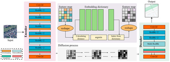
Figure 3.
The details of the mechanism of mapping into latent space. Firstly, when mapping the images into latent space, we use a couple of networks to compress x to a feature vector . Meanwhile, we propose KL-reg and VQ-reg regularization to avoid high variance, including a reshaping module, calculating module, embedding dictionary and index of the dictionary.
The pretrained VQGAN includes three components: encoder, decoder and image regularization. Given an image in Domain A, the encoder maps a into a latent representation , where , and the decoder reconstructs the image y from the latent space . Especially, the downsample factor of the encoder is , and we will discuss different values of f’s influence.
Meanwhile, to avoid the arbitrarily high-variance during the sampling stage, we propose two kinds of regularization, KL-reg and VQ-reg. To make feature vectors towards a standard normal, we implement a slight KL-penalty. The VQ-reg, which is a vector quantization layer in the decoder, firstly reshapes the feature vector. Then, compared with the distance between it and the vector in the embedding dictionary, we can select the appropriate feature vector with the minimum distance in the dictionary.
3.3. End-to-End Translation Model Based on DMs
We have designed an end-to-end diffusion model for the remote sensing images-to-maps translation task, which is distinguished from exiting methods. For accurate generation, we control the maximum variance in the diffusion process. Additionally, in the sampling stage, the MapGen-Diff reduces the uncertainty in every step for denoising with the start of raw RS images.
3.3.1. Forward Process for Diffusion
Different from initiating the generation process with a pure Gaussian noise, we take the reference input y as the denoising condition and diffusion destination. Thus, we obtain sample data . According to the theorem mentioned in [39], the time-reversed SDE can be obtained via an evolution if a conditional probability is formed by Equation (1).
where is a vector-valued drift function, g is a scalar-valued diffusion coefficient, is a Wiener process, and . Thus, given the endpoint remote sensing image , we find the solution of Equation (1) to reconstruct maps.
However, the general denoising diffusion bridge model is constructed based on various stochastic processes, which may cause the randomness of the output quality. Thus, inspired by [21], we employ the strategy of Brownian motion, which makes the mathematical process more understandable. For each time in the diffusion process, given at and ending point , the process can be formulated as
where T (total steps) is a hyper-parameter of the diffusion process.
It has been mentioned in VPSDE [3] and DDPM [20] that assuming that is intended to follow a standard normal distribution, it is essential to maintain the variance at the identity level.
However, according to Equation (2), the variance at time can be extremely large if the total steps T increase. Therefore, in order to obtain relatively controllable variance, a novel strategy inspired by Brownian motion can be designed as
From Equation (4), the largest variance at the middle time can be controlled below . Then, the variance drops until . Therefore, we introduce an influence factor s that can scale to control the diversity of the sampling results.
In addition to the marginal distribution in Equation (3), another key step is to deduce the forward transition probability . Through computing each step , the transition probability can be derived as
When the diffusion process arrives at the forward endpoint, we can obtain and . Thus, the translation between Domain A and B is defined.
3.3.2. Reverse Process for Denoising
According to previous works, the start of the reverse process is pure noise sampling from the Gaussian distribution. The generation process is aimed to eliminate noise step by step to obtain an objective result.
However, for specific RSMT tasks, this conditional translation contains many uncontrollable diversities. The reverse process of our proposed model starts from the source domain, which means that . Below is the main computation that aims to predict based on .
where we use neural networks with the parameter obtained from training to predict the mean value . The variance plays an important role in high-quality results and is related to the objective function. In the reverse process, we start at the reference y sampled from the remote sensing image domain.
3.4. Loss Function
For specific RSMT tasks, we design a novel loss function of MapGen-Diff, including the diffusion process objective and geometric constraint, which can be express as
where the is the Evidence Lower Bound, and is the transformation consistency regularization loss for geographic constraints. is designed to control the trade-off between losses.
3.4.1. Evidence Lower Bound
The optimizing objective of diffusion process in our model which can be formulated as
Since we fixed the endpoint, , the first term in Equation (8) can be viewed as a constant. Combined with Equations (3) and (5), the formulation in the second term can be derived by the Bayes theorem and the Markov chain property:
where the key point is calculating the . Meanwhile, the neural network is the key step to predict the noise instead of predicting the whole . Then, can be formulated as
where the computation details of , and are presented in [21].
Therefore, according to the above analysis, the training objective can be simplified as
where present the mean value of , y and noise . is a factor designed above. can be considered as random noise to increase randomness. is a noise function that varies with time step t. The entire formulation expresses that based on the reference y, original input and noise , we can optimize the mod, enabling it to generate samples that more closely approximate the target distribution.
3.4.2. TCR Loss
Consistency regularization (CR) is a strategy to force the model to preserve uniform predictions in the face of various data perturbations [52], which is employed in the classification task based on semi-supervision. Additionally, some studies based on contrastive learning [53] utilize some embedding samples to enhance data diversity and are similar to CR. Therefore, inspired by CR, we apply transformation consistency regularization (TCR) to conduct the RMST. Through a geometrical transformation, MapGen-Diff is more focused on the geometrical consistency with more data diversity.
In Figure 2, we have a geometrical transformation function . The data sample , where is sampled from a source domain A (RS images) and belongs to a target domain B (online maps). Applying the transformation function , and are data pairs from Domains and . We represent the diffusion process as . In the denoising process, we take a and as the start point , and we obtain target maps . Thus, the TCR loss formula can be express as
where through a transformation, such as rotation, flipping and cropping, we enforce our model to keep a consistency between the reconstructed maps from the given reference remote sensing images.
4. Results
In this experimental section, we firstly make a brief description of the data source, experimental setups, evaluation metrics and selected baselines. Then, through the objective scores and subjective visual analysis, we compare our MapGen-Diff with other competitive methods. Finally, some ablation studies are conducted to validate the effectiveness of each component in our framework.
4.1. Datasets and Setups
In order to verify the effectiveness of the proposed model, we conducted experiments on the Los Angeles datasets and Toronto datasets [27], which comprise both remote sensing images and the corresponding maps sourced from Google Maps. The images are from the Digital Orthophoto Map and are in visible wavelengths, comprising buildings, roads, waterway and vegetation. To ensure the feasibility of the experiment, the data were cleaned to remove the adverse impacts caused by illumination and weather.
- Los Angeles datasets: We selected a dataset comprising 4,631 pairs of samples from the urban area of Los Angeles, USA. The RS images comprise urban streets and buildings. These Los Angeles images are scraped from Google Maps, corresponding to a spatial resolution of 2.15 m per pixel.
- Toronto datasets: The Toronto datasets, which we accessed and downloaded at zoom level 17 on Google Maps, come with the same spatial resolution and more diverse ground elements. In order to remove the “dirty data”, we selected 3200 paired samples, which were accurately matched.
Upon analysis of the two datasets, we found that there were inconsistencies in the coloration of the same ground elements or unmatched sample pairs. After removing the unmatched samples, we solely acquired paired samples to support the accurate generation of online maps. Table 1 shows the details of the two datasets. Figure 4 presents some samples of the two datasets.

Table 1.
Details of the two widely open datasets in experiments for remote sensing images to online map translations.
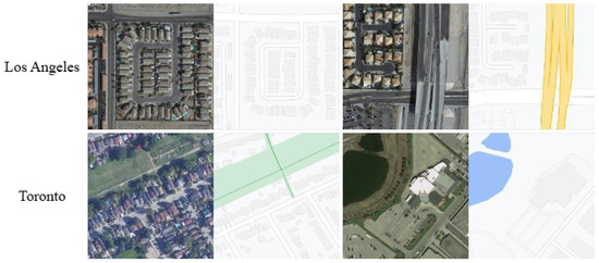
Figure 4.
Some selected pairs of samples from the two datasets used in this article.
We present the MapGen-Diff network design in Figure 2. During the training stage, we set the whole diffusion steps T as 1000, and we determined the number of sampling steps as 200. In the downsampling stage of the encoder, we set as the default. As described in Equation (7), we set . We carried out all of the training on a PC with an Intel Core (TM) i7-13700H CPU @ 2.40 GHz, 16GB RAM, and a GeForce GTX 4090 GPU.
4.2. Evaluation Metrics
The evaluation metrics of generative models can be classified into two categories. The first one is based on the target images such as PSNR and MSE [54]. The second one does not use target images such as FID [55]. The objective of RSMT is to generate images from target domains. Therefore, we have selected RMSE, SSIM and ACC as evaluation metrics.
4.2.1. Root Mean Square Error
The root mean square error (RMSE) [56] calculates the difference between variables. It can reflect the pixel error to evaluate image quality. When the calculated value is approximately close to 0, the generated image is closer to the original image. Assume that the collection of generated images is , and the original images can be expressed as ; the RMSE’s general function is expressed by
4.2.2. Structural Similarity
SSIM [57] is an evaluation metric for describing the similarity between two domain images. We compare the luminance (mean), contrast (variance) and structure (covariance) of each pixel block to evaluate the similarity between different domains images. The adopted formula is
where represents the average of , represents the average of . represents the variance of , represents the variance of y, and represents the covariance between and y. and are constant values adopted to stabilize the computation. L is the range of pixel values. Generally, , and . The SSIM ranges from 0 to 1, where a value closer to 1 indicates a higher similarity between two images.
4.2.3. Pixel Accuracy
The valuation metric Pixel Accuracy (ACC) is used to calculate the pixels level precision of a generated image. The original RGB value is described as , and the predicted RGB value of the translated maps is ; if the max is set as 5 according to [58], , it is considered that the translator is accurate.
4.3. Baselines
To verify the effectiveness of our MapGen-Diff, we selected some typical image translation methods (Pix2pix [11], CycleGAN [12] and AIME [59]), as well as several out-performance RSMT methods (MapGenGAN [18], SMAPGAN [26] and Semi-MapGen [27]). Pix2pix represents a significant advance in the domain of image translation based on fully matched sample pairs. ATME overcomes the instability of training in GAN models and combines denoising machinery from DMs. It also needs matched training samples. Both Cyclegan and MapGenGAN employ cyclic consistency loss to achieve unpaired images to map translations. SMAPGAN and Semi-MapGen utilize the semi-supervised learning strategy, including a knowledge extension-based learning network.
For the supervised learning model, we use the fully paired samples from the aforementioned datasets. Then, all matched samples are shuffled randomly in each of the datasets, which are used in the CycleGAN and MapGenGAN. According to [26,27], we can select a ratio of 1:4 for the paired and unpaired samples on the two datasets, comprising SMAPGAN and Semi-MapGen.
4.4. Comparisons with Baselines
In order to demonstrate the efficacy of our method, we compare our MapGen-Diff with six typical models for RMST in both objective and subjective results.
4.4.1. Quantitative Results
In order to assess objective metrics of MapGen-Diff in comparison with other baseline methods, three image quality evaluation metrics were employed. Table 2 and Table 3, respectively, display the quantitative results for each model applied to the Los Angeles and Toronto datasets. The top scores are highlighted in a bold font, with the second-best scores being underlined. Our model’s performance is compared with those of supervised, unsupervised and semi-supervised approaches.

Table 2.
Quantitative scores of different methods on three image evaluation metrics on LA datasets. (Highest score marked in bold font; sub-optimal score underlined).

Table 3.
Quantitative scores of different methods on three image evaluation metrics on Toronto datasets. (Highest score marked in bold font; sub-optimal score underlined).
First of all, to verify the statistical significance of our results, we selected 100 samples randomly to implement a significance test with the average metrics. In Figure 5, the analysis of the sampled data distribution via box plots is shown, illustrating that the scores of sampled data are uniformly distributed. After removing the abnormal values, we implemented a one sample t-test to validate the statistical significance between the samples and the population. The p-values are LA: RMSE—, SSIM—, ACC—; Toronto: RMSE—, SSIM—, and ACC—p = . All metrics satisfy , which means that there is no significant difference between the sampled data and the population. Therefore, through a sufficient statistical analysis, the reliability of our metric results can be validated.
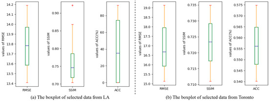
Figure 5.
The data distributions of the samples in LA datasets and Toronto datasets.
In general, the MapGen-Diff outperforms the other baselines almost in every metric while exhibiting sub-optimal performance of the ACC on LA datasets. It is acknowledged that the ACC involves a pixel-wise comparison of RGB values between the original and translated images. Therefore, a slight difference in RGB values can affect the ACC score. On the LA datasets, most of the map area is based on a white background, which implies that minor fluctuations in RGB values result in negligible variations in color perception. Through an analysis of the qualitative results, there is a slight difference in the colorization in the background between the generated maps and the ground truth. Therefore, sub-optimal performance is acceptable without having to compromise the quality of generated images.
Specifically, firstly, for LA datasets, our model achieves the highest scores for both RMSE and SSIM metrics. While our methodology slightly lags behind ATME in the ACC metric, it still achieves an impressive score of up to . In particular, MapGen-Diff yields a 5–30% improvement in the RMSE and a 2–17% increase in the SSIM in comparison to the previous methods.
Secondly, within the Toronto datasets, our proposed MapGen-Diff framework demonstrates a marked superiority over all comparative baselines across three distinct performance metrics. Compared with the average performance of other baselines, our model achieves a notable increase of 29% in the RMSE, an 8% improvement in the SSIM, and a 14% higher ACC. Our model exhibits enhanced stability when evaluated on the Toronto datasets, as opposed to its performance on the LA datasets. This enhanced stability suggests a higher degree of robustness and reliability of diffusion models, which may be attributed to variations in data complexity and geographic features represented in Toronto datasets.
4.4.2. Qualitative Results
The qualitative outcomes are presented in Figure 6 and Figure 7. We selected a subset of samples from the generated maps across two distinct datasets for demonstration. In the comparative figures, each column corresponds to the input remote sensing images, the ground truth, maps generated by our MapGen-Diff and generated maps of other baseline models.
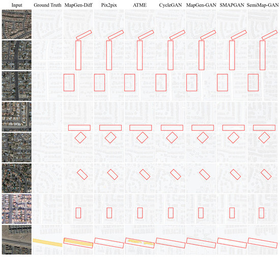
Figure 6.
Qualitative comparisons of generated online maps by different approaches on LA datasets (red rectangles: out-performance).
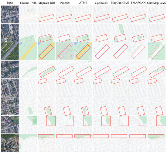
Figure 7.
Qualitative comparisons of generated online maps by different approaches on Toronto datasets (red rectangles: out-performance).
In general, MapGen-Diff demonstrates a marked advantage over other baselines in terms of vegetation and waterway color recognition, as well as regarding the boundaries of roads and buildings. This enhanced performance can be attributed to the geometrical constraints and the diversity afforded by the diffusion model, which contribute to the visually striking results of our approach. The incorporation of these elements has led to MapGen-Diff’s exceptional visual performance, which distinguishes it from its counterparts in the RSMT.
Specifically, Figure 6 shows the generated maps of LA datasets. The unsupervised methods, CycleGAN and MapGen-GAN, generate some blurred maps. Semi-supervised methods are more effective at reconstructing the shapes of roads and buildings but cannot recognize the difference in feature elements correctly. Pix2pix and ATME are sightly inferior to MapGen-Diff in terms of the overall visual quality.
In Toronto datasets, which includes a variety of geographic elements, comprising streets, motorways, vegetation and waterways, it is more challenging to generate corresponding images with clear boundaries and shapes. From Figure 7, MapGen-Diff can clarify different ground elements with both diversity and accuracy. The supervised methods, Pix2pix and ATME, generate some maps with semantic distortions, which are slightly inferior to our method in dealing with the colorization of different features. The unsupervised and semi-supervised methods exhibit limitations in terms of the accuracy of different regions’ classification. Moreover, for slight differences between remote sensing images and ground truths, our approach facilitates the learning of a color representation that closely mirrors remote sensing images.
4.5. Ablation Study
In order to confirm the performance of individual components within our framework, we executed ablation studies for an in-depth analysis of MapGen-Diff. We firstly removed the TCR loss function to evaluate the impact of geometrical constraint in the remote sensing field (MapGen-Diff-no-). Then, the encoder and decoder were removed to validate whether the latent space contributed to the quality of the generated images ((MapGen-Diff-no-latent).
The objective results are represented in Table 4. Under the same setup as in other parameters, the default model, MapGen-Diff, outperforms MapGen-Diff-no- on all metrics. This is attributed to the effectiveness of the geometric constraint of transformation consistency regularization. Compared with the single diffusion process, our method improves geometric precision and reduces semantic distortion. Moreover, we noticed that the performance of MapGen-Diff-no-Latent is slightly higher than MapGen-Diff on the RMSE and ACC in LA datasets, and on the SSIM in Toronto datasets. However, the subsequent qualitative results demonstrate that MapGen-Diff-no-Latent generates blurred maps, which indicates that the scores of MapGen-Diff-no-Latent are misdirected by poor fidelity.

Table 4.
Quantitative scores of ablation studies on two datasets with each core component (highest score marked in bold font; sub-optimal score underlined).
Next, we represent the qualitative evaluation via a visual representation in Figure 8. The removal of TCR loss results in blurring and a distorted outline of the urban roads and some buildings. As marked in red rectangles, it can be observed that there are segmentation anomalies, particularly affecting critical roads and the vegetation of MapGen-Diff-no-. Upon ceasing the mapping to latent space, we observed that the resultant image exhibited a degree of blurriness. Furthermore, the outline of the generated buildings suffered from pixel-level distortion, with some vegetation parts being absent. Although MapGen-Diff-no- achieves relatively excellent scores on quantitative metrics, the blurring and distortion results are unacceptable. The results indicate that the latent space and TCR loss function can extract more features from RS images and enhance the visual fidelity from diverse dimensions.
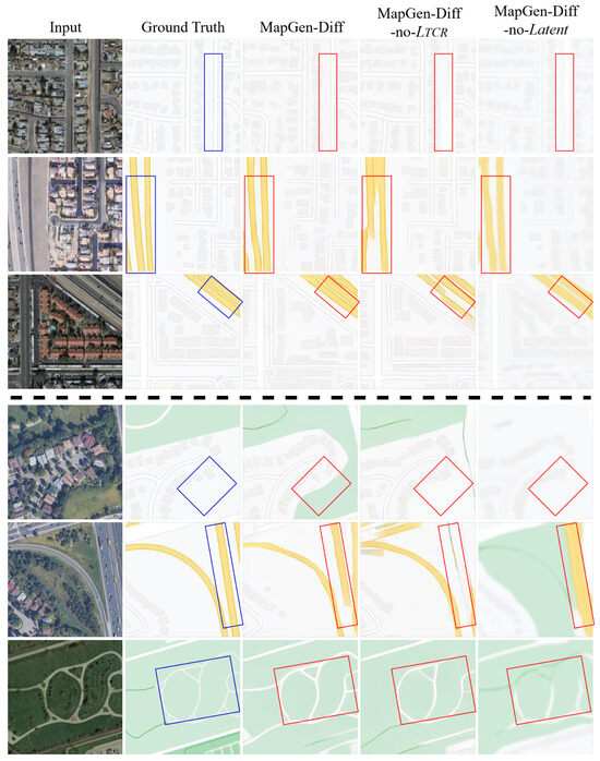
Figure 8.
Various visualization results of the ablation study with four selected sample in each dataset. The upper three rows are from LA datasets and the ones below are from Toronto datasets.
4.6. Robustness Analysis
According to Equation (4), maximum variance is a core factor in the forward process of the training stage, which can influence the robustness of the model within the quality of the generated maps. Therefore, in order to explore the maximum variance impact on the results’ diversity, we scale the maximum variance with several experiments taken on to investigate the influence of on the performance of our MapGen-Diff.
The objective scores are reported in Table 5. The results demonstrate that the maximum variance significantly influences the performance. Specifically, when the numerical values are relatively small, such as MapGen-Diff- = 0, the image generation outcomes are generally satisfactory, with only minor contour distortions being observed. As the values increase, such as MapGen-Diff-=2 and MapGen-Diff- = 4, the diversity of the diffusion model at is enhanced, which may result in significant distortions.

Table 5.
Objective results of varying on two datasets (highest score marked in bold font; sub-optimal score underlined).
Figure 9 also reflects more graphic visualization results. In Figure 9a, as the increase in the value of occurs, there is some distortion in the corresponding maps. Specifically, when , the model cannot capture the key features of remote sensing images, such as highways and waterways. Moreover, we plot the entropy images of the corresponding maps in Figure 9b. The red area represents that there are more local details. Regarding the models with a lower , the entropy map is more similar to the ground truth. Therefore, through the analysis of the varying , it is proved that the maximum variance can directly influence the reference results. Especially in the classification of different elements, more constraints should be employed when the is large.
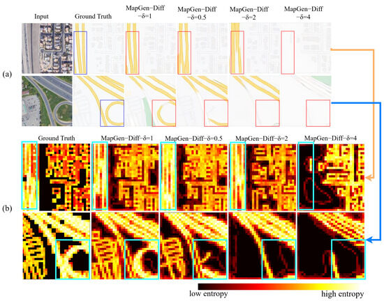
Figure 9.
Qualitative results involving varying the maximum variance . Part (a) demonstrates the visualization of the generated map; part (b) represents the entropy image of the translated maps based on the different values of .
5. Discussion
With the denoising diffusion process in the latent space, it can extract more features in order to achieve controllable and high-fidelity generation. However, there were still exiting issues with the downsampling factor and sampling steps that required an in-depth discussion, which motivated us to conduct extensive experiments, as follows. Moreover, we discussed some limitations and future directions.
5.1. Influence of the Downsampling Factor
When we compare the MapGen-Diff with different downsampling factors , from Figure 10, there are some interesting results within different f values. In the red rectangle, the model with higher values seems to generate maps which are more in line with subjective judgments. However, there are more mistakes represented in the blue rectangles.
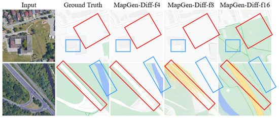
Figure 10.
Qualitative results with different values of the downsampling factor.
Therefore, we quantitatively analyze the diversity and accuracy of generated maps under different sampling factors illustrated by bar and line charts. In Figure 11, the bar chart represents diversity, which uses the average discrepancy between images. With higher values of f, the diversity increases ( in LA, in Toronto). The line chart indicates the accuracy for which we employ the SSIM as the evaluation metric. The accuracy of generated maps declines, about (), as the f increasing. The analysis yields conclusions consistent with the aforementioned qualitative results. The higher downsampling factor leads to more abstract generation.
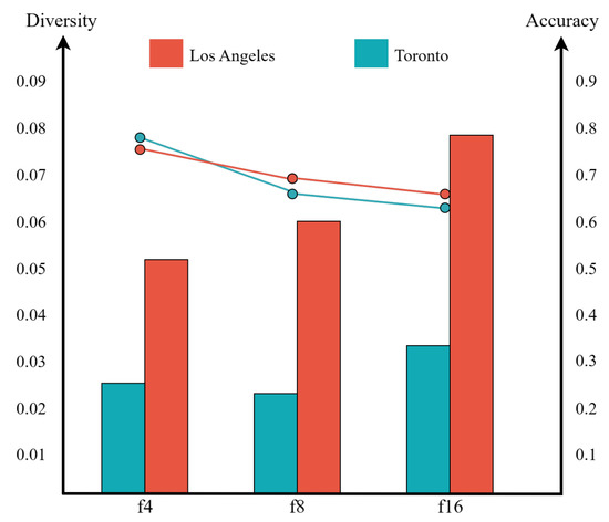
Figure 11.
Qualitative comparisons with different values of the downsampling factor on two datasets. The bar chart represents the experimental results of diversity. The line chart represents the experimental results of accuracy.
Understanding deep learning models has always been a hot topic in academia. This section provides an elementary exploration of the model’s capabilities under different sampling factors. The higher values of the downsampling factor indicates the wider global receptive fields, which are attributed to extracting more abstract features from RS images. However, due to the fact that our MapGen-Diff only employs TCR loss as a constraint, the generated maps tend to deviate from the constraint of the input image.
5.2. Effect of Sampling Steps
We explore the influence of the hyper-parameter and sampling steps on the quality of generated maps. In Figure 12, we record the three metric results with different steps in the two datasets.

Figure 12.
The results of different values of sampling steps. Representation of metric values on LA datasets. Representation of metric values on Toronto datasets.
On LA datasets, when the values of sampling steps range from 20 to 100 (fewer than the default 200 steps), the performance of our model decreases with the increasing values. Until the sampling steps equals to 200, the metric scores become higher than the other steps. However, MapGen-Diff suffers from poor performance when the step size is 1000.
In Toronto datasets, the results are similar with those obtained on LA datasets, where 200 steps demonstrate optimal performance in both RMSE and SSIM metrics, achieving a decisive advantage in comparison to other steps.
In summary, sampling steps are hyper-parameters that directly affect the quality of image generation. In the reverse process, different sampling steps represent noise with varying degrees of randomness. Our experiments revealed that the numbers of steps of 20 and 200 both yield satisfactory performance. Therefore, the automated determination of hyper-parameters also seems to be a subject worth investigating.
5.3. Limitations
In deep learning neural networks, time complexity and space complexity are significant metrics for evaluating the performance of a model. Thus, we employed two representative metrics, computation cost/floating points (FLOPs) and model parameters, to measure the complexity of our model. Table 6 shows details of the comparison with other methods. Due to the backbone of the U-Net structure in MapGen-Diff, our model has a larger number of parameters. Additionally, diffusion models usually generate results via multiple sampling steps, which need a higher computation cost in FLOPs. Diffusion models are generally more computationally complex than other generative models, but their advantage in generative quality often makes this complexity acceptable.

Table 6.
Comparison of the complexity with other baselines and test time taken for generating 70 square kilometers, and a 1:2000 scale of a map based in Toronto datasets.
Next, we compare the test time taken to translate remote sensing images into online maps with real-world Toronto datasets. In Table 6, it is shown that it takes about 20 min to generate maps from a seventy-square-kilometer urban area. According to [60], it takes about one day to make a map of 0.5 square kilometers and a 1:2000 scale manually. Therefore, compared with traditional methods, the translation time of MapGen-Diff is acceptable. While the computation cost is relatively large, we acquire higher-quality online maps instead.
6. Conclusions
In this article, we introduce diffusion models to conduct an RMST task, which is a novel exploration. For map generation, MapGen-Diff is extensively capable to achieve high-fidelity generation based on a denoising diffusion bridge model. Inspired by the strategy of Brownian motion, we improve the general DMs to make a trade-off between the diversity and accuracy of generated maps. Through mapping images into latent space, the network can capture more features of ground elements. Meanwhile, with the help of transformation regularization consistency loss, MapGen-Diff attends to generate maps with clearer boundaries and colorization. Following comprehensive experimental comparisons on two widely used datasets, our model has demonstrated the capacity to produce generations that are more competitive than those achieved by previous approaches, both in objective and subjective terms.
For future works, we intend to collect extensive image datasets, encompassing a variety of geographical features and different regions. Through pretraining on large-scale data, we aim to develop a robust translation model. Additionally, we hope to integrate prior knowledge provided by a discriminative model to better regulate our generation results.
Author Contributions
Conceptualization, methodology, investigation, data curation, formal analysis, and writing—original draft preparation, J.T.; conceptualization, methodology, investigation, and writing—review and editing, H.C.; supervision, H.C., J.W. and M.M. All authors have read and agreed to the published version of the manuscript.
Funding
This work was supported in part by the National Natural Science Foundation of China under grants Nos. 42471403, 42101435, 42101432 and 62106276.
Data Availability Statement
The data presented in this study are available upon request from the corresponding author.
Acknowledgments
The authors would like to thank the anonymous referees for their valuable comments and helpful suggestions.
Conflicts of Interest
The authors declare no conflicts of interest.
References
- Ablameyko, S.V.; Beregov, B.S.; Kryuchkov, A.N. Computer-aided cartographical system for map digitizing. In Proceedings of the 2nd International Conference on Document Analysis and Recognition (ICDAR’93), Tsukuba, Japan, 20–22 October 1993; pp. 115–118. [Google Scholar]
- Hang, R.; Liu, Q.; Hong, D.; Ghamisi, P. Cascaded recurrent neural networks for hyperspectral image classification. IEEE Trans. Geosci. Remote Sens. 2019, 57, 5384–5394. [Google Scholar] [CrossRef]
- Song, Y.; Sohl-Dickstein, J.; Kingma, D.P.; Kumar, A.; Ermon, S.; Poole, B. Score-based generative modeling through stochastic differential equations. arXiv 2020, arXiv:2011.13456. [Google Scholar]
- Li, W.; Hsu, C.Y. Automated terrain feature identification from remote sensing imagery: A deep learning approach. Int. J. Geogr. Inf. Sci. 2020, 34, 637–660. [Google Scholar] [CrossRef]
- Li, X.; Wang, Y.; Zhang, L.; Liu, S.; Mei, J.; Li, Y. Topology-enhanced urban road extraction via a geographic feature-enhanced network. IEEE Trans. Geosci. Remote Sens. 2020, 58, 8819–8830. [Google Scholar] [CrossRef]
- Wu, Y.; Xu, L.; Chen, Y.; Wong, A.; Clausi, D.A. TAL: Topography-aware multi-resolution fusion learning for enhanced building footprint extraction. IEEE Geosci. Remote Sens. Lett. 2022, 19, 1–5. [Google Scholar] [CrossRef]
- Hosseinpour, H.; Samadzadegan, F.; Javan, F.D. CMGFNet: A deep cross-modal gated fusion network for building extraction from very high-resolution remote sensing images. ISPRS J. Photogramm. Remote Sens. 2022, 184, 96–115. [Google Scholar] [CrossRef]
- Zhang, J.; Lin, S.; Ding, L.; Bruzzone, L. Multi-scale context aggregation for semantic segmentation of remote sensing images. Remote Sens. 2020, 12, 701. [Google Scholar] [CrossRef]
- Goodfellow, I.; Pouget-Abadie, J.; Mirza, M.; Xu, B.; Warde-Farley, D.; Ozair, S.; Courville, A.; Bengio, Y. Generative adversarial networks. Commun. ACM 2020, 63, 139–144. [Google Scholar] [CrossRef]
- Mirza, M.; Osindero, S. Conditional generative adversarial nets. arXiv 2014, arXiv:1411.1784. [Google Scholar]
- Isola, P.; Zhu, J.Y.; Zhou, T.; Efros, A.A. Image-to-Image Translation with Conditional Adversarial Networks. In Proceedings of the 2017 IEEE Conference on Computer Vision and Pattern Recognition (CVPR), Honolulu, HI, USA, 21–26 July 2017; pp. 5967–5976. [Google Scholar] [CrossRef]
- Zhu, J.Y.; Park, T.; Isola, P.; Efros, A.A. Unpaired Image-to-Image Translation Using Cycle-Consistent Adversarial Networks. In Proceedings of the 2017 IEEE International Conference on Computer Vision (ICCV), Venice, Italy, 22–29 October 2017; pp. 2242–2251. [Google Scholar] [CrossRef]
- Ganguli, S.; Garzon, P.; Glaser, N. GeoGAN: A conditional GAN with reconstruction and style loss to generate standard layer of maps from satellite images. arXiv 2019, arXiv:1902.05611. [Google Scholar]
- Song, J.; Li, J.; Chen, H.; Wu, J. RSMT: A Remote Sensing Image-to-Map Translation Model via Adversarial Deep Transfer Learning. Remote Sens. 2022, 14, 919. [Google Scholar] [CrossRef]
- Xu, J.; Zhou, X.; Han, C.; Dong, B.; Li, H. SAM-GAN: Supervised learning-based aerial image-to-map translation via generative adversarial networks. ISPRS Int. J. Geo-Inf. 2023, 12, 159. [Google Scholar] [CrossRef]
- Phatangare, S.; Khalifa, M.M.; Kharche, S.; Khatib, A.; Kshirsagar, A. Satellite Image to Map Translation using GANs. Grenze Int. J. Eng. Technol. (GIJET) 2024, 10. [Google Scholar]
- Dhariwal, P.; Nichol, A. Diffusion models beat gans on image synthesis. Adv. Neural Inf. Process. Syst. 2021, 34, 8780–8794. [Google Scholar]
- Song, J.; Li, J.; Chen, H.; Wu, J. MapGen-GAN: A Fast Translator for Remote Sensing Image to Map Via Unsupervised Adversarial Learning. IEEE J. Sel. Top. Appl. Earth Obs. Remote Sens. 2021, 14, 2341–2357. [Google Scholar] [CrossRef]
- Xiao, Z.; Kreis, K.; Vahdat, A. Tackling the generative learning trilemma with denoising diffusion gans. arXiv 2021, arXiv:2112.07804. [Google Scholar]
- Ho, J.; Jain, A.; Abbeel, P. Denoising diffusion probabilistic models. Adv. Neural Inf. Process. Syst. 2020, 33, 6840–6851. [Google Scholar]
- Li, B.; Xue, K.; Liu, B.; Lai, Y. BBDM: Image-to-Image Translation with Brownian Bridge Diffusion Models. In Proceedings of the 2023 IEEE/CVF Confernece Computer Vision and Pattern Recognition (CVPR), Vancouver, BC, Canada, 17–24 June 2022; pp. 1952–1961. [Google Scholar]
- Rombach, R.; Blattmann, A.; Lorenz, D.; Esser, P.; Ommer, B. High-resolution image synthesis with latent diffusion models. In Proceedings of the IEEE/CVF Conference on Computer Vision and Pattern Recognition, New Orleans, LA, USA, 18–24 June 2022; pp. 10684–10695. [Google Scholar]
- Zhu, J.Y.; Zhang, R.; Pathak, D.; Darrell, T.; Efros, A.A.; Wang, O.; Shechtman, E. Toward multimodal image-to-image translation. Adv. Neural Inf. Process. Syst. 2017, 30. [Google Scholar]
- Yi, Z.; Zhang, H.; Tan, P.; Gong, M. DualGAN: Unsupervised Dual Learning for Image-to-Image Translation. In Proceedings of the 2017 IEEE International Conference on Computer Vision (ICCV), Venice, Italy, 22–29 October 2017; pp. 2868–2876. [Google Scholar] [CrossRef]
- Kim, T.; Cha, M.; Kim, H.; Lee, J.K.; Kim, J. Learning to discover cross-domain relations with generative adversarial networks. In Proceedings of the International Conference on Machine Learning, Sydney, Australia, 6–11 August 2017; pp. 1857–1865. [Google Scholar]
- Chen, X.; Chen, S.; Xu, T.; Yin, B.; Peng, J.; Mei, X.; Li, H. SMAPGAN: Generative Adversarial Network-Based Semisupervised Styled Map Tile Generation Method. IEEE Trans. Geosci. Remote Sens. 2021, 59, 4388–4406. [Google Scholar] [CrossRef]
- Song, J.; Chen, H.; Du, C.; Li, J. Semi-MapGen: Translation of Remote Sensing Image Into Map via Semisupervised Adversarial Learning. IEEE Trans. Geosci. Remote Sens. 2023, 61, 1–19. [Google Scholar] [CrossRef]
- Saharia, C.; Chan, W.; Chang, H.; Lee, C.; Ho, J.; Salimans, T.; Fleet, D.; Norouzi, M. Palette: Image-to-image diffusion models. In Proceedings of the ACM SIGGRAPH 2022 Conference Proceedings, Vancouver, BC, Canada, 7–11 August 2022; pp. 1–10. [Google Scholar]
- Wang, T.; Zhang, T.; Zhang, B.; Ouyang, H.; Chen, D.; Chen, Q.; Wen, F. Pretraining is all you need for image-to-image translation. arXiv 2022, arXiv:2205.12952. [Google Scholar]
- Zhang, L.; Rao, A.; Agrawala, M. Adding conditional control to text-to-image diffusion models. In Proceedings of the IEEE/CVF International Conference on Computer Vision, Paris, France, 1–6 October 2023; pp. 3836–3847. [Google Scholar]
- Yang, L.; Zhang, Z.; Song, Y.; Hong, S.; Xu, R.; Zhao, Y.; Zhang, W.; Cui, B.; Yang, M.H. Diffusion Models: A Comprehensive Survey of Methods and Applications. ACM Comput. Surv. 2023, 56, 1–39. [Google Scholar] [CrossRef]
- Nichol, A.Q.; Dhariwal, P. Improved denoising diffusion probabilistic models. In Proceedings of the International Conference on Machine Learning, Virtual, 18–24 July 2021; pp. 8162–8171. [Google Scholar]
- Sohl-Dickstein, J.; Weiss, E.; Maheswaranathan, N.; Ganguli, S. Deep unsupervised learning using nonequilibrium thermodynamics. In Proceedings of the International Conference on Machine Learning, Lille, France, 6–11 July 2015; pp. 2256–2265. [Google Scholar]
- Song, Y.; Ermon, S. Generative modeling by estimating gradients of the data distribution. Adv. Neural Inf. Process. Syst. 2019, 32. [Google Scholar]
- Song, Y.; Ermon, S. Improved techniques for training score-based generative models. Adv. Neural Inf. Process. Syst. 2020, 33, 12438–12448. [Google Scholar]
- Song, Y.; Durkan, C.; Murray, I.; Ermon, S. Maximum likelihood training of score-based diffusion models. Adv. Neural Inf. Process. Syst. 2021, 34, 1415–1428. [Google Scholar]
- Doob, J.L.; Doob, J. Classical Potential Theory and Its Probabilistic Counterpart; Springer: Berlin/Heidelberg, Germany, 1984; Volume 262. [Google Scholar]
- Liu, X.; Wu, L.; Ye, M.; Liu, Q. Let us build bridges: Understanding and extending diffusion generative models. arXiv 2022, arXiv:2208.14699. [Google Scholar]
- Zhou, L.; Lou, A.; Khanna, S.; Ermon, S. Denoising Diffusion Bridge Models. arXiv 2023, arXiv:2309.16948. [Google Scholar]
- De Bortoli, V.; Thornton, J.; Heng, J.; Doucet, A. Diffusion schrödinger bridge with applications to score-based generative modeling. Adv. Neural Inf. Process. Syst. 2021, 34, 17695–17709. [Google Scholar]
- Saharia, C.; Ho, J.; Chan, W.; Salimans, T.; Fleet, D.J.; Norouzi, M. Image super-resolution via iterative refinement. IEEE Trans. Pattern Anal. Mach. Intell. 2022, 45, 4713–4726. [Google Scholar] [CrossRef]
- Nichol, A.; Dhariwal, P.; Ramesh, A.; Shyam, P.; Mishkin, P.; McGrew, B.; Sutskever, I.; Chen, M. Glide: Towards photorealistic image generation and editing with text-guided diffusion models. arXiv 2021, arXiv:2112.10741. [Google Scholar]
- Parmar, G.; Singh, K.K.; Zhang, R.; Li, Y.; Lu, J.; Zhu, J.Y. Zero-shot Image-to-Image Translation. In Proceedings of the ACM SIGGRAPH 2023 Conference Proceedings, Los Angeles, CA, USA, 6–10 August 2023. [Google Scholar]
- Sasaki, H.; Willcocks, C.G.; Breckon, T.P. Unit-ddpm: Unpaired image translation with denoising diffusion probabilistic models. arXiv 2021, arXiv:2104.05358. [Google Scholar]
- Choi, J.; Kim, S.; Jeong, Y.; Gwon, Y.; Yoon, S. Ilvr: Conditioning method for denoising diffusion probabilistic models. In Proceedings of the CVF International Conference on Computer Vision (ICCV), Montreal, QC, Canada, 10–17 October 2021; pp. 14347–14356. [Google Scholar]
- Meng, C.; He, Y.; Song, Y.; Song, J.; Wu, J.; Zhu, J.Y.; Ermon, S. Sdedit: Guided image synthesis and editing with stochastic differential equations. arXiv 2021, arXiv:2108.01073. [Google Scholar]
- Zhao, M.; Bao, F.; Li, C.; Zhu, J. Egsde: Unpaired image-to-image translation via energy-guided stochastic differential equations. Adv. Neural Inf. Process. Syst. 2022, 35, 3609–3623. [Google Scholar]
- Wu, C.H.; De la Torre, F. A latent space of stochastic diffusion models for zero-shot image editing and guidance. In Proceedings of the IEEE/CVF International Conference on Computer Vision, Paris, France, 2–6 October 2023; pp. 7378–7387. [Google Scholar]
- Sun, S.; Wei, L.; Xing, J.; Jia, J.; Tian, Q. SDDM: Score-Decomposed Diffusion Models on Manifolds for Unpaired Image-to-Image Translation. In Proceedings of the 40th International Conference on Machine Learning, ICML 2023, Honolulu, HI, USA, 23–29 July 2023; PMLR, 2023. Volume 202, pp. 33115–33134. [Google Scholar]
- Esser, P.; Rombach, R.; Ommer, B. Taming transformers for high-resolution image synthesis. In Proceedings of the IEEE/CVF Conference on Computer Vision and Pattern Recognition, Nashville, TN, USA, 20–25 June 2021; pp. 12873–12883. [Google Scholar]
- Mustafa, A.; Mantiuk, R.K. Transformation consistency regularization–a semi-supervised paradigm for image-to-image translation. In Proceedings of the Computer Vision–ECCV 2020: 16th European Conference, Glasgow, UK, 23–28 August 2020; Proceedings, Part XVIII 16. Springer: Berlin/Heidelberg, Germany, 2020; pp. 599–615. [Google Scholar]
- Laine, S.; Aila, T. Temporal ensembling for semi-supervised learning. arXiv 2016, arXiv:1610.02242. [Google Scholar]
- Park, T.; Efros, A.A.; Zhang, R.; Zhu, J.Y. Contrastive learning for unpaired image-to-image translation. In Proceedings of the Computer Vision–ECCV 2020: 16th European Conference, Glasgow, UK, 23–28 August 2020; Proceedings, Part IX 16. Springer: Berlin/Heidelberg, Germany, 2020; pp. 319–345. [Google Scholar]
- Willmott, C.J.; Matsuura, K. Advantages of the mean absolute error (MAE) over the root mean square error (RMSE) in assessing average model performance. Clim. Res. 2005, 30, 79–82. [Google Scholar] [CrossRef]
- Heusel, M.; Ramsauer, H.; Unterthiner, T.; Nessler, B.; Hochreiter, S. Gans trained by a two time-scale update rule converge to a local nash equilibrium. Adv. Neural Inf. Process. Syst. 2017, 30. [Google Scholar]
- Chai, T.; Draxler, R.R. Root mean square error (RMSE) or mean absolute error (MAE)?–Arguments against avoiding RMSE in the literature. Geosci. Model Dev. 2014, 7, 1247–1250. [Google Scholar] [CrossRef]
- Wang, Z.; Bovik, A.C.; Sheikh, H.R.; Simoncelli, E.P. Image quality assessment: From error visibility to structural similarity. IEEE Trans. Image Process. 2004, 13, 600–612. [Google Scholar] [CrossRef]
- Fu, H.; Gong, M.; Wang, C.; Batmanghelich, K.; Zhang, K.; Tao, D. Geometry-Consistent Generative Adversarial Networks for One-Sided Unsupervised Domain Mapping. In Proceedings of the 2019 IEEE/CVF Conference on Computer Vision and Pattern Recognition (CVPR), Long Beach, CA, USA, 15–20 June 2019; pp. 2422–2431. [Google Scholar] [CrossRef]
- Solano-Carrillo, E.; Rodriguez, A.B.; Carrillo-Perez, B.; Steiniger, Y.; Stoppe, J. Look ATME: The Discriminator Mean Entropy Needs Attention. In Proceedings of the 2023 IEEE/CVF Conference on Computer Vision and Pattern Recognition, Vancouver, BC, Canada, 17–24 June 2023; pp. 787–796. [Google Scholar]
- Jones, C.B. Geographical Information Systems and Computer Cartography; Routledge: London, UK, 2014. [Google Scholar]
Disclaimer/Publisher’s Note: The statements, opinions and data contained in all publications are solely those of the individual author(s) and contributor(s) and not of MDPI and/or the editor(s). MDPI and/or the editor(s) disclaim responsibility for any injury to people or property resulting from any ideas, methods, instructions or products referred to in the content. |
© 2024 by the authors. Licensee MDPI, Basel, Switzerland. This article is an open access article distributed under the terms and conditions of the Creative Commons Attribution (CC BY) license (https://creativecommons.org/licenses/by/4.0/).