Progressive Unsupervised Domain Adaptation for Radio Frequency Signal Attribute Recognition across Communication Scenarios

Abstract

As the development of low-altitude economies and aerial countermeasures continues, the safety of unmanned aerial vehicles becomes increasingly critical, making emitter identification in remote sensing practices more essential. Effective recognition of radio frequency (RF) signal attributes is a prerequisite for identifying emitters. However, due to diverse wireless communication environments, RF signals often face challenges from complex and time-varying wireless channel conditions. These challenges lead to difficulties in data collection and annotation, as well as disparities in data distribution across different communication scenarios. To address this issue, this paper proposes a progressive maximum similarity-based unsupervised domain adaptation (PMS-UDA) method for RF signal attribute recognition. First, we introduce a noise perturbation consistency optimization method to enhance the robustness of the PMS-UDA method under low signal-to-noise conditions. Subsequently, a progressive label alignment training method is proposed, combining sample-level maximum correlation with distribution-level maximum similarity optimization techniques to enhance the similarity of cross-domain features. Finally, a domain adversarial optimization method is employed to extract domain-independent features, reducing the impact of channel scenarios. The experimental results demonstrate that the PMS-UDA method achieves superior recognition performance in automatic modulation recognition and RF fingerprint identification tasks, as well as across both ground-to-ground and air-to-ground scenarios, compared to baseline methods.

1. Introduction

With the increasing emphasis on unmanned aerial vehicle (UAV) technology in fields such as low-altitude economies [1,2,3,4] and offensive and defensive confrontations [5,6], the threat posed by highly dynamic electromagnetic targets is on the rise. Consequently, efficient electromagnetic awareness of high-maneuverability targets in complex environments has become an urgent requirement for remote sensing practices. The identification of electromagnetic targets fundamentally relies on recognizing the attributes of the radio frequency (RF) signals they emit. This encompasses both signal and device attribute recognition. Signal attributes include modulation type [7,8], signal bandwidth [9], center frequency [10,11], etc., whereas device attributes are primarily defined by RF fingerprints [12,13,14].

With the advancement of machine learning, deep-learning-based methods for RF signal attribute recognition have made significant progress in recent years, bringing new vitality to electromagnetic emitter identification. Despite these strides, the propagation of RF signals often faces challenges due to dynamic, time-varying, and complex wireless channel conditions across various spatiotemporal contexts, such as air-to-ground (A2G) channels in low-altitude economic zones [15,16,17]. Unlike ground-to-ground (G2G) scenarios, A2G channels are influenced by multiple factors, including transceiver mobility, fluctuating atmospheric conditions, and diverse terrains. These influences impact RF signal propagation, introducing variability and uncertainty in the data distribution. Consequently, traditional deep learning models, trained on single-scenario data, struggle to adapt and accurately identify RF signal characteristics across different scenarios. Additionally, the diversity and complexity of communication environments complicate effective RF signal capture and labeling, amplifying the challenges in cross-scenario deep-learning-based RF signal attribute recognition.

Facing the challenges of distribution discrepancies in signal data across scenarios and the scarcity of data and labels, traditional deep learning methods struggle to cope effectively. Transfer learning (TL) provides a solution by allowing the migration of prior knowledge from one scenario to another, thereby enhancing the performance of RF signal attribute recognition in new environments [18,19,20]. Specifically, domain adaptation within TL facilitates knowledge acquisition in the target domain by leveraging insights from the source domain [21,22]. This strategy addresses challenges due to distribution discrepancies and label scarcity in the target domain [23,24,25,26]. Therefore, domain adaptation methods not only optimize the use of existing data resources but also adapt to changes in signal attribute distribution across different scenarios, offering new opportunities and challenges to the field of RF signal attribute recognition.

In the realm of RF signal attribute recognition, domain-adaptation-based methods have demonstrated considerable promise and benefits. Bu et al. [27] introduced an innovative adversarial TL framework to address the challenge of automatic modulation recognition (AMR) amid shifting data distributions and limited signal data availability. This method leverages a synergy of adversarial training and knowledge transfer, aiming to minimize disparities in data distributions through adversarial training while simultaneously exploiting knowledge transfer to extract prior knowledge from the source domain. To tackle the issue of divergent data distributions between test and training sets, Liu et al. [28] presented a radio frequency fingerprint identification (RFFI) technique for long-term specific transmitter identification. This method achieves domain alignment between source and target domain samples through unsupervised domain adaptation, thereby diminishing the intra-class variability of deep features and alleviating the misclassification of edge samples in the target domain. Nonetheless, the current TL-based methods for RF signal attribute recognition often employ a random selection of training samples from the target domain. This practice can result in decreased correlation between samples across source and target domains, as well as a reduction in the distribution similarity of batch domains, which hinders the alignment and extraction of domain-invariant features.

To address the aforementioned challenges across scenarios, this paper focuses on the study of cross-scenario RF signal attribute recognition. We propose a progressive maximum similarity-based unsupervised domain adaptation (PMS-UDA) method for RF signal attribute recognition across G2G and A2G channel scenarios. Initially, to enhance the model’s robustness in diverse noisy environments, a noise perturbation consistency optimization method is introduced. This method leverages the subtle feature differences induced by random noise in the signals of the target domain to learn feature representations under various signal-to-noise ratio (SNR) conditions. Subsequently, addressing the challenge of effectively learning feature similarities at both the sample and distribution levels in high-dimensional spaces, we introduce a progressive label alignment training (PLAT) method. This method optimizes the learning of maximum sample-level correlation and distribution-level similarity. Finally, to mitigate the impact of channel differences on feature learning, a domain adversarial optimization method is incorporated. This method employs adversarial learning to extract domain-invariant RF signal attribute features, enhancing the generalizability and accuracy of the model across diverse operational scenarios.

The main contributions of this paper are as follows:

(1)

A noise perturbation consistency optimization learning method is introduced to utilize slight noise perturbations during training, enhancing the model’s robustness to various SNR conditions and improving the performance at low SNRs.

(2)

We propose a progressive label alignment training method, which, combined with optimization for maximizing sample-level correlation and distribution-level similarity, effectively enhances the similarity between the feature distributions of the source and target domains, thus increasing the cross-scenarios adaptability of RF signal attribute features.

(3)

Utilization of domain adversarial optimization learning methods to extract domain-invariant features, significantly reducing the impact of channel scenario differences on recognition outcomes.

(4)

Compared to baseline methods, the proposed method demonstrates superior performance in AMR and RFFI tasks across G2G and A2G channel scenarios.

The remainder of this paper is organized as follows. Section 2 presents the problem formulation and the corresponding solutions developed for addressing the challenges in wireless communication systems. Section 3 explores the network architectures of backbone employed for feature extraction. Section 4 delves into the proposed UDA method. Section 5 presents the experimental setup and analyzes the outcomes of the proposed UDA method. Finally, Section 6 concludes the paper with a summary of our findings. The list of abbreviations and notations used in the article are presented in

Table 1. Abbreviations and Notations.

Abbreviations	Notations
RF	Radio frequency
PMS-UDA	Progressive maximum similarity-based unsupervised domain adaptation
UAV	Unmanned aerial vehicle
A2G	Air-to-ground
G2G	Ground-to-ground
TL	Transfer learning
AMR	Automatic modulation recognition
RFFI	Radio frequency fingerprint identification
SNR	Signal-to-noise ratio
PLAT	Progressive label alignment training
AWGN	Additive white Gaussian noise
MSCNs	Multi-scale correlation networks
MPDFormer	Multi-periodicity dependency transformer
NPCL	Noise perturbation constancy loss
SMCL	Sample-level maximum correlation loss
DMSL	Distribution-level maximum similarity loss
KL	Kullback-Leibler
DAL	Domain adversarial loss
SDR	Software-defined radio
MPC	Multi-path component
t-SNE	t-distributed stochastic neighbor embedding
I,Q	in-phase and quadrature components of signal

and

Table 2. Notations and Definitions.

Notation	Definition	Notation	Definition
$R\left(t\right)$	Received signal	$\theta$	Trainable parameters of backbone model
$\mathcal{H}\left(t\right)$	Channel impulse response	$x_s$, $x_t$	Normalized signals of source and target domain
$S\left(t\right)$	Transmitted signal	$y_s$	Truth category labels from source domain
$N\left(t\right)$	Additive white Gaussian noise	$x_t^{\prime }$	Normalized signals of target domain with noise perturbation
${\alpha }_k$	Amplitude of the k-th tap	${∥·∥}_2$	${\ell }_2$ norm
${\tau }_k$	Path delay of the k-th tap	$n_0\left(t\right)$	Additive white Gaussian noise
${\omega }_k$	Frequency of the k-th tap	$f_{\theta }\left(x_{t,i}\right)$	Feature map of original signal from target domain
${\varphi }_k$	Phase offset of the k-th tap	$f_{\theta }\left(x_{t,i}^{\prime }\right)$	Feature map of perturbed signal from target domain
$\mathcal{L}(·)$	Loss function	$f_{\theta }\left(x_i\right)$	Feature map of the signal samples
${\mathcal{L}}_{npcl}$	Noise perturbation consistency loss	$P_{G2G}(X,Y)$	Joint probability of G2G scenario
${\mathcal{L}}_{smcl}$	Sample-level maximum correlation loss	$P_{A2G}(X,Y)$	Joint probability of A2G scenario
${\mathcal{L}}_{dmsl}$	Distribution-level maximum similarity loss	${\mathcal{M}}_{*}$	The expression for the mean distribution
${\mathcal{L}}_{dal}$	Domain adversarial loss	$KL(·)$	KL divergence
${\mathcal{L}}_{ce}$	Cross entropy loss	$JS(·)$	JS divergence
$\rho$	Balancing factor for ${\mathcal{L}}_{npcl}$	${\mu }_s,{\mu }_t$	Mean of $f_{\theta }\left(x_{s,i}\right)$ and $f_{\theta }\left(x_{t,i}\right)$, respectively
$\beta$	Balancing factor for ${\mathcal{L}}_{smcl}$	$tr(·)$	Trace of a matrix
$\gamma$	Balancing factor for ${\mathcal{L}}_{dal}$	n	Total number of signal samples
$\eta$	Balancing factor for ${\mathcal{L}}_{ce}$	$n_s,n_t$	Number of samples in the source and target domain
S, T	Source and target domain	$n_i$	Number of correctly recognized samples for the i-th attribute
$P_S(x,y)$	Joint probability distribution within the source domain	$\lambda$	Weighting parameter of the squared correlation coefficient
$P_T(x,y)$	Joint probability distribution within the target domain	$d_i$	Binary domain label
${\sum }_{j\in Y}$	Aggregation across categorical labels	$D_{\psi }$	Domain adversarial network
$y_{i,j}$	Truth category labels	$\psi$	Trainable parameters of the adversarial network
${\widehat{y}}_{i,j}$	Predicted category labels	$\epsilon$	Trainable parameters of the classification network
X, Y	Input and Label space of signal	$f_c(·)$	Classifier of the RF signal attribute recognition
$R_S^{emp}\left(f_{\theta }\left(x\right)\right)$	Empirical risk within the source domain	C	Total number of attribute categories
$R_T^{emp}\left(f_{\theta }\left(x\right)\right)$	Empirical risk within the target domain	N	Total number of samples in the test set

, respectively.

2. Problem Formulation and Solution

2.1. Problem Formulation

In the wireless communication systems, the interaction between transmitted signals and the channel through which they propagate is of paramount importance. The received signal, $R\left(t\right)$, is formulated as the convolution of the transmitted signal $S\left(t\right)$ with the channel impulse response $\mathcal{H}\left(t\right)$, in addition to additive white Gaussian noise (AWGN), $N\left(t\right)$, represented as

$$\begin{array}{c}\hfill \mathbf{R}\left(t\right)=\mathcal{H}\left(t\right)\ast \mathbf{S}\left(t\right)+\mathbf{N}\left(t\right).\end{array}$$

(1)

This model captures the essence of signal propagation in wireless channels, including the effects of multipath fading and noise. Equation (1) is also described in the form of multiple taps:

$$\begin{array}{c}\hfill \mathbf{R}\left(m\right)=\sum _k{\alpha }_{k}s(m-{\tau }_k)e^{-j{\omega }_k{\tau }_k+{\varphi }_k}+n\left(m\right),\end{array}$$

(2)

where ${\alpha }_k$, ${\tau }_k$, ${\omega }_k$, and ${\varphi }_k$ denote the amplitude, path delay, frequency, and phase offset of the kth tap, respectively.

The spatial scope of the G2G channel under urban topography and geomorphology discussed is relatively small, with the relative movement speed and height difference between the transceivers being negligible. In contrast, the A2G channel in an urban environment comprises a direct path and a ground-reflected path, with a probabilistic existence of 3-9 multipath components. Additionally, due to the high flight speed of drones, the A2G channel exhibits significant Doppler effects compared to the new G2G scenarios. Generally, the A2G channel scenario covers a wider spatial range, leading to relatively severe path loss.

Therefore, the constructed G2G and A2G channel models exhibit significant differences within their channel parameters, specifically in ${\alpha }_k$, ${\tau }_k$, ${\omega }_k$, and ${\varphi }_k$. Furthermore, the distribution of $n\left(m\right)$ may also vary. These variations lead to different distributions of the RF signal data across channel models. To better describe the problem of domain adaptation, we denote the signal input to the deep model as X, which represents the RF signal $R\left(m\right)$ that has undergone wireless channel effects. Meanwhile, Y is used to denote the label of the signal X. Suppose the sample data of the RF signal in the G2G scenario follow the distribution $P_{G2G}(X,Y)$, denoted as $(x,y)\sim P_{G2G}(X,Y)$, similarly, the sample data of the RF signal in the A2G scenario adhere to the distribution $P_{A2G}(X,Y)$, represented as $(x,y)\sim P_{A2G}(X,Y)$. Due to these distributional differences in the sample data of RF signal across scenarios, deep-learning-based methods for RF signal attribute recognition experience a significant performance degradation in cross-scenario applications.

2.2. Problem Solution

In practical wireless communication scenarios, we can obtain samples of RF signals along with their corresponding labels in familiar environments. However, the task often extends to performing similar tasks in new communication scenarios. Based on the previous analysis of two communication channel conditions, a distribution discrepancy exits between the sample spaces of RF signals in these two scenarios. Moreover, in the new communication scenarios, only a few of RF signal samples are known, with no access to the corresponding labels.

2.2.1. Traditional Deep Learning Paradigm

In the traditional deep learning, the empirical risk within the source domain is represented as

$$\begin{array}{cc}\hfill R_S^{emp}\left(f_{\theta }\left(x\right)\right)& ={\mathbb{E}}_{(x,y)\sim P_S(x,y)}\left[\mathcal{L}(f_{\theta }\left(x\right),y)\right]\hfill \\ \hfill & =\sum _{y\in \mathcal{Y}}{\int }_{\mathcal{X}}\mathcal{L}(f_{\theta }\left(x\right),y)P_S(x,y)dx,\hfill \end{array}$$

(3)

where $\mathcal{L}(f_{\theta }\left(x\right),y)$ denotes the loss function, $\theta$ denotes the trainable parameters of deep model $f_{\theta }\left(x\right)$, and $P_S(x,y)$ symbolizes the joint probability distribution within the source domain. The summation ${\sum }_{y\in \mathcal{Y}}$ represents the aggregation across categorical labels, signifying that the risk is assessed over all possible outcomes within the label space $\mathcal{Y}$. Concurrently, the integral ${\int }_{\mathcal{X}}$ is performed over the continuous input space $\mathcal{X}$, capturing the expected loss across the entire data distribution within the source domain. This dual operation of summation and integration is pivotal in computing the comprehensive expected risk, ensuring the model’s performance is evaluated over both the entire input domain and the categorical outcomes.

For the unfamiliar target domain, the empirical risk is represented as

$$\begin{array}{cc}\hfill R_T^{emp}\left(f_{\theta }\left(x\right)\right)& ={\mathbb{E}}_{(x,y)\sim P_T(x,y)}\left[\mathcal{L}(f_{\theta }\left(x\right),y)\right]\hfill \\ \hfill & =\sum _{y\in \mathcal{Y}}{\int }_{\mathcal{X}}\mathcal{L}(f_{\theta }\left(x\right),y)P_T(x,y)dx.\hfill \end{array}$$

(4)

However, the labels of target domain, $y_T\in {\mathcal{Y}}_T$, are unavailable. Therefore, the traditional deep learning paradigm is incapable of effectively addressing the task with the unlabeled sample in the target domain.

2.2.2. Deep Domain Adaptation Paradigm

The solution to domain adaptation involves learning a model $f_{\theta }(·)$ that performs well on a target domain T, characterized by a low risk $R_T\left(f_{\theta }\left(x\right)\right)$, using labeled data from a source domain S and unlabeled data from a target domain T. To enhance the model’s generalizability across different distributions, both domains are leveraged simultaneously.

The fundamental expression for the risk on the source domain is given in Equation (3). The risk in the target domain, $R_T\left(f_{\theta }\left(x\right)\right)$, can be conceptually derived as the expectation of the loss function with respect to the target distribution:

$$\begin{array}{cc}\hfill R_T\left(f_{\theta }\left(x\right)\right)& ={\mathbb{E}}_{(x,y)\sim P_T(x,y)}\left[\mathcal{L}(f_{\theta }\left(x\right),y)\right]\hfill \\ \hfill & =\sum _{y\in \mathcal{Y}}{\int }_{\mathcal{X}}\mathcal{L}(f_{\theta }\left(x\right),y)P_T(x,y)dx\hfill \\ \hfill & =\sum _{y\in \mathcal{Y}}{\int }_{\mathcal{X}}\mathcal{L}(f_{\theta }\left(x\right),y){\displaystyle \frac{P_T(x,y)}{P_S(x,y)}}{P}_S(x,y)dx\hfill \\ \hfill & ={\mathbb{E}}_{(x,y)\sim P_S(x,y)}\left[{\displaystyle \frac{P_T(x,y)}{P_S(x,y)}}\mathcal{L}(f_{\theta }\left(x\right),y)\right],\hfill \end{array}$$

(5)

where ${\displaystyle \frac{P_T(x,y)}{P_S(x,y)}}$ is a domain adaptation factor in the transformation, which serves to reconcile the distributions discrepancy of two domains.

For the practical implementation of training a model under this paradigm, the empirical risk on the target domain is minimized by evaluating

$$\begin{array}{c}\hfill R_T^{emp}\left(f_{\theta }\left(x\right)\right)={\displaystyle \frac{1}{n}}\sum _{i=1}^n\mathcal{L}(f_{\theta }\left(x_i\right),y_i){\displaystyle \frac{p_T(x_i,y_i)}{p_S(x_i,y_i)}},\end{array}$$

(6)

where $(x_i,y_i)$ are samples drawn from the target domain distribution $P_T(x,y)$, and n represents the number of samples. Crucial to this process is estimating the ratio, commonly referred to as the domain adaptation factor.

To address the issue of unlabeled data in the target domain, it is necessary to minimize the loss function $\mathcal{L}(·)$ while maximizing the similarity ${\displaystyle \frac{P_T(x,y)}{P_S(x,y)}}$ between the source and target domains.

3. Network Architectures for Task of Feature Extraction

To more effectively extract features relevant to two types of RF signal attributes, we introduce two distinct deep-learning-based network architectures from our previous works, namely, the multi-scale correlation networks (MSCNs) [29] and multi-periodicity dependency transformer (MPDFormer) [30].

3.1. Multi-Scale Correlation Networks for AMR Task

In the task of AMR, we incorporate our previous work [29] with the MSCNs network architecture for extracting the features from modulated signals in the cross-scenarios. The MSCNs can effectively suppress noise and enhance the features of the modulated signals, thereby achieving the AMR task under low SNRs. The network architecture of MSCNs for the AMR task is shown in

Table 3. Layout of MSCNs network architecture for AMR task. kFLOPs refers to kilo floating-point operations, LSWT denotes learnable stationary wavelet transform, MSC denotes multi-scale correlation, SAFS denotes subband-adaptive frequency selection, FS-ResNet denotes frequency selection ResNet, GAP is global average pooling, and FC is full connection.

Layer	Output Dimension	Number of Parameters	kFLOPs
Input	$1024\times 2$	-	0
LSWT	$1024\times 4\times 5$	120	245.8
MSC	$1024\times 4\times 5$	-	143.4
SAFS	$1024\times 2\times 6$	426	130.5
FS-ResNet	$512\times 16$	2256	3313.3
FS-ResNet	$256\times 32$	6544	5426.9
FS-ResNet	$128\times 64$	23,312	10,675.1
GAP	64	-	8.2

.

3.2. Multi-Periodicity Dependency Transformer for RFFI Task

In the task of RF signal attribute recognition, we have introduced a Transformer network architecture based on a periodicity–dependency attention mechanism, termed MDPFormer. The MPDFormer utilizes a spectrum offset-based periodic embedding representation to enhance the differentiation of intrinsic features. We explore the complexities of the periodicity–dependency attention mechanism, which incorporates both inter-period and intra-period attention frameworks. This mechanism enables the effective extraction of both long-range and short-range periodicity-dependent features, thereby emphasizing feature distinctions while simultaneously reducing the disturbances introduced by background noise and features with weak periodicity.

The network architecture of MPDFormer is shown in

Table 4. Layout of MPDFormer network architecture for RFFI task.

Layers	Output Dimension	Parameters	kFLOPs
Input	1024 × 2	–	–
Periodic Embedding Representation	16 × 128	–	13,799.4
Projection	16 × 128	16,512
Scaling	16 × 128	–
Positional Encoding	16 × 128	–
Encoding Layers	16 × 128	1,193,472
Transpose	128 × 16	–
GAP	128 × 1	–
Squeeze	128	–
Periodic Embedding Representation	25 × 84	–	9626.4
Projection	25 × 84	7140
Scaling	25 × 84	–
Positional Encoding	25 × 84	–
Encoding Layers	25 × 84	517,104
Transpose	84 × 25	–
GAP	84 × 1	–
Squeeze	84	–
Periodic Embedding Representation	8 × 256	–	27,004.9
Projection	8 × 256	65,792
Scaling	8 × 256	–
Positional Encoding	8 × 256	–
Encoding Layers	8 × 256	4,746,240
Transpose	256 × 8	–
GAP	256 × 1	–
Squeeze	256	–
Concatenation	468	–	0.1
Adaptive Fusion	468	144

.

4. Method

The unsupervised domain adaptation method described is depicted in Figure 1. Initially, the method utilizes the MSCNs and MPDFormer networks to process the input signal samples from both the source and target domains, thereby deriving feature representations. Subsequently, the extracted features are leveraged to achieve cross-scenario domain adaptation and RF signal attribute recognition. This is accomplished through a series of learning strategies, including noise perturbation consistency learning, sample-level maximum correlation learning, distribution-level maximum similarity learning, domain adversarial learning, and source-domain cross-entropy optimization learning. Additionally, a balancing factor is introduced to adjust the gradient weight of these learning strategies during the backpropagation optimization process. The formulation of the learning strategies with loss function proposed is as follows:

$$\begin{array}{cc}\hfill J(\theta ,\psi ,\epsilon ;x_s,x_t,{x^{\prime }}_t,y_s)=& \rho {\mathcal{L}}_{npcl}(\theta ;x_t,{x^{\prime }}_t)+\beta {\mathcal{L}}_{smcl}(\theta ;x_s,x_t)+(1-\beta ){\mathcal{L}}_{dmsl}(\theta ;x_s,x_t)\hfill \\ \hfill +& \gamma {\mathcal{L}}_{dal}(\theta ,\psi ;x_s,x_t)+\eta {\mathcal{L}}_{ce}(\theta ,\epsilon ;x_s,y_s),\hfill \end{array}$$

(7)

where $\theta$, $\psi$, and $\epsilon$ represent the set of trainable parameters of backbone, adversarial network and task classification network, respectively. The variables $x_s$, $x_t$, $x_t^{\prime }$, and $y_s$ correspond to the normalized signals from source domain, target domain, target domain with noise perturbation, and the labels from source domain, respectively. ${\mathcal{L}}_{npcl}$, ${\mathcal{L}}_{smcl}$, ${\mathcal{L}}_{dmsl}$, ${\mathcal{L}}_{dal}$, and ${\mathcal{L}}_{ce}$ represent the noise perturbation constancy loss, sample-level maximum correlation loss, distribution-level maximum similarity loss, domain adversarial loss, and cross-entropy loss, respectively. Additionally, $\rho$, $\beta$, $\gamma$, and $\eta$ are the balancing factors for their respective loss functions.

We proceed to detail the following learning strategies: noise perturbation consistency comparison learning, sample-level maximum correlation learning, distribution-level maximum similarity learning, domain adversarial learning, and source-domain cross-entropy optimization learning.

4.1. Noise Perturbation Consistency Learning

Labeling a vast array of signal samples in a novel environment is challenging, yet even a modest collection of signal samples can be an invaluable source of data. Consequently, to make the most of the numerous unlabeled signal samples present in a new setting and, concurrently, to discern the intrinsic features of RF signal attributes amidst the interference of noise perturbation while mitigating the adverse effects of noise on RF signals, this section introduces the noise perturbation constancy loss (NPCL). This loss function is predicated on the principle of noise perturbation consistency and employs comparative learning to facilitate the effective extraction of features.

Noise perturbation consistency learning serves as an unsupervised learning technique designed to enhance a model’s resilience to noise and fluctuations in input data. It operates by incorporating minor noise perturbation into the training process and demanding that the model yield consistent predictions for both the pristine and the noise-perturbed data. This method compels the model to learn the genuine distribution and properties of the data rather than merely internalizing the noise and anomalies present in the training set. Incorporating such losses aids in reducing model overfitting and enhances its capacity to generalize to new, unseen data. The formulation for incorporating noise perturbation into the signal is outlined as follows:

$$\begin{array}{c}\hfill x^{\prime }\left(t\right)=x\left(t\right)+n_0\left(t\right),\end{array}$$

(8)

where $n_0\left(t\right)$ denotes additive white Gaussian noise.

The noise perturbation consistency loss is quantified through the metric of cosine similarity. Let the model parameters be denoted by $\theta$, with the original source and target domain signal data represented by $x_s$ and $x_t$, respectively. The corresponding signal data perturbed by noise are $x_s^{\prime }$ and $x_t^{\prime }$, respectively. The model’s feature extraction outputs for both the original and perturbed data are given by $f_{\theta }\left(x\right)$ and $f_{\theta }\left(x^{\prime }\right)$, respectively. Consequently, the cosine similarity loss can be formulated as the discrepancy between the cosine distances of the pairs of feature vectors:

$$\begin{array}{c}\hfill {\mathcal{L}}_{npcl}(\theta ;x_t,x_t^{\prime })=1-{\displaystyle \frac{1}{n_t}}\sum _{j=1}^{n_t}{\displaystyle \frac{f_{\theta }\left(x_{t,j}\right)·f_{\theta }\left({x^{\prime }}_{t,j}\right)}{\parallel f_{\theta }\left(x_{t,j}\right){\parallel }_2· {\parallel f_{\theta }\left({x^{\prime }}_{t,j}\right)\parallel }_2}},\end{array}$$

(9)

where $f_{\theta }\left(x_{t,j}\right)$ and $f_{\theta }\left({x^{\prime }}_{t,j}\right)$ denote the feature map of original and perturbed signal from target domain, · denotes the inner product of vectors, and ${∥·∥}_2$ denotes their L2 norms, respectively.

Minimizing the cosine similarity loss compels the model to generate similar feature extraction outcomes for both pristine and perturbed data, thereby enhancing the model’s robustness and capacity for generalization. This process effectively curbs the model’s tendency to overfit on the noise and fluctuations within the training dataset, guiding the model to more accurately capture the intrinsic feature distribution of the data. In contrast to traditional supervised learning paradigms, this method places a greater emphasis on the model’s generalization capabilities, equipping the model to exhibit enhanced resilience when confronted with unfamiliar data or varied environmental contexts. Moreover, the incorporation of noise perturbation consistency loss is cost-effective, as it leverages data transformation and perturbation techniques during training, eliminating the need for additional labeling efforts.

4.2. Sample-Level Maximum Correlation Learning

To effectively diminish the divergence among samples sharing identical labels, this section introduces the sample-level maximum correlation loss (SMCL). The sample-level maximum correlation loss is designed to refine the distinctiveness of the feature representation by amplifying the correlation among samples that belong to the same class. This strategy is instrumental in enhancing the model’s proficiency in the domain of RF signal attribute recognition. The incorporation of a sample-level correlation constraint within the loss function enables SMCL to efficiently mitigate intra-class variance, thereby improving the model’s proficiency in discerning the intra-class distribution. Consequently, during the training phase, the model is compelled to integrate samples with the same label into a closely-knit feature space.

The sample-level maximum correlation loss is crafted to cultivate a feature representation that is more generalizable by emphasizing the correlation between analogous samples cross both the source and target domains. The formulation of this loss function is expressed as follows:

$$\begin{array}{c}\hfill r(\theta ,x_s,x_t)={\displaystyle \frac{1}{n}}\sum _{i=1}^n{\displaystyle \frac{tr\left({[f_{\theta }\left(x_{s,i}\right)-{\mu }_s]}^T[f_{\theta }\left(x_{t,i}\right)-{\mu }_t]\right)}{\parallel f_{\theta }\left(x_{s,i}\right)-{\mu }_s\parallel ·\parallel f_{\theta }\left(x_{t,i}\right)-{\mu }_t\parallel }},\end{array}$$

(10)

$$\begin{array}{c}\hfill {\mathcal{L}}_{smcl}(\theta ;x_s,x_t)=1-\lambda r(\theta ,x_s,x_t),\end{array}$$

(11)

where $x_s$ and $x_t$ denote the feature means of the samples in the source and target domains, respectively; $f_{\theta }\left(x_{s,i}\right)$ and $f_{\theta }\left(x_{t,i}\right)$ denote the feature representations of the samples $x_{s,i}$ and $x_{t,i}$, respectively; ${\mu }_s$ and ${\mu }_t$ denote the mean of $f_{\theta }\left(x_{s,i}\right)$ and $f_{\theta }\left(x_{t,i}\right)$, respectively; $tr(·)$ represents the trace of a matrix; n is the total number of signal samples; $\lambda$ is a weighting parameter used to control the influence of the squared correlation coefficient; and we set $\lambda =0.5$ empirically. The sample-level maximum correlation loss is distinguished by its efficacy in narrowing the distributional disparities between the source and target domains, thereby enhancing the model’s generalization capabilities on the target domain.

4.3. Distribution-Level Maximum Similarity Learning

The distribution-level maximum similarity loss (DMSL) reduces the distributional difference between the source and target domains by maximizing the similarity of the signal feature distributions of the source and target domains taken within each batch to improve the generalization performance of the model on the target domain. DMSL improves the generalization performance of the model on the target domain by using the Jensen–Shannon (JS) divergence [31] to optimize the feature distributions of the two domains and improve their similarity. In contrast to the Kullback–Leibler (KL) divergence [32], JS divergence is symmetric and smooth, which addresses the problem that KL divergence is asymmetric and may produce infinite values if the probability distributions do not support the same events. It is used to measure the similarity between two probability distributions, providing a score ranging between 0 and 1, where 0 means the distributions are identical and 1 means the distributions are completely different.

Assuming that the distributions of the source and target domain data features in the probability space are $f_{\theta }\left(x_s\right)$ and $f_{\theta }\left(x_t\right)$, respectively, the JS divergence of these two distributions is defined through the KL divergence of their mean distribution M. The expression for the mean distribution M is

$$\begin{array}{c}\hfill M={\displaystyle \frac{1}{2}}[f_{\theta }\left(x_s\right)+f_{\theta }\left(x_t\right)].\end{array}$$

(12)

Therefore, JS divergence is defined as

$$\begin{array}{c}\hfill JS(f_{\theta }\left(x_s\right),f_{\theta }\left(x_t\right))={\displaystyle \frac{1}{2}}KL(f_{\theta }\left(x_s\right)\Vert M)+{\displaystyle \frac{1}{2}}KL(f_{\theta }\left(x_t\right)\Vert M),\end{array}$$

(13)

where $KL(P \Vert Q)$ is the KL divergence of Q to P, and it can be expressed as

$$\begin{array}{c}\hfill KL(P \Vert Q)=\sum _{x\in \mathcal{X}}P\left(x\right)log\left({\displaystyle \frac{P\left(x\right)}{Q\left(x\right)}}\right),\end{array}$$

(14)

where $\mathcal{X}$ denotes the set of all possible events in distributions P and Q. This leads to the mathematical expression of DMSL as follows:

$$\begin{array}{cc}\hfill & {\mathcal{L}}_{dmsl}(\theta ;x_s,x_t)\hfill \\ \hfill & ={\displaystyle \frac{1}{2}}\sum _{x\in \mathcal{X}}\left[f_{\theta }\left(x_s\right)log\left({\displaystyle \frac{2f_{\theta }\left(x_s\right)}{f_{\theta }\left(x_s\right)+f_{\theta }\left(x_t\right)}}\right)+f_{\theta }\left(x_t\right)log\left({\displaystyle \frac{2f_{\theta }\left(x_t\right)}{f_{\theta }\left(x_s\right)+f_{\theta }\left(x_t\right)}}\right)\right].\hfill \end{array}$$

(15)

4.4. Domain Adversarial Learning

The domain adversarial loss (DAL) serves as an optimization metric aimed at mitigating discrepancies in data distributions between the source and target domains. Its objective is to facilitate the seamless transfer of knowledge acquired from the source domain during model training to the target domain. DAL fosters the extraction of domain-invariant features by incorporating an adversarial mechanism, thereby diminishing the model’s susceptibility to performance degradation due to domain variations.

Employing this strategy, the model transcends its proficiency in the source domain, extending its high-accuracy performance to the unlabeled target domain. The conceptual foundation of DAL is rooted in adversarial training, which aims to align the feature distributions of the source and target domains through iterative optimization. This alignment bolsters the model’s capability to accurately recognize RF signal attributes across various scenarios.

The domain adversarial loss operates through a binary domain discriminator, which is a domain classification network designed to discern the origin of input feature maps—whether from the source or target domain. The network architecture of this domain discriminator is illustrated in

Table 5. Layout of domain adversarial network architecture.

Layer	Output Dimension
	AMR	RFFI
Input	64	468
Linear	128	128
SELU	128	128
Dropout	128	128
Linear	128	128
SELU	128	128
Dropout	128	128
Linear	2	2

. The domain adversarial loss is expressed as follows:

$$\begin{array}{c}\hfill {\mathcal{L}}_{dal}(\theta ,\psi ;x)=-{\displaystyle \frac{1}{n}}\sum _{i=1}^n\left[d_{i}log{D}_{\psi }\left(f_{\theta }\left(x_i\right)\right)+(1-d_i)log(1-D_{\psi }\left(f_{\theta }\left(x_i\right)\right))\right],\end{array}$$

(16)

where $d_i$ is a binary domain label, with $d_i=1$ for source domain samples and $d_i=0$ for target domain samples; $D_{\psi }$ is the domain adversarial network; $\psi$ is the parameters of the adversarial network; x denotes the signal samples from source and target domain; and $f_{\theta }\left(x_i\right)$ is the feature maps extracted by the backbone network.

Throughout the training process, the objective of the domain domain classifier is to maximally confuse the adversarial network regarding the provenance of the features, thereby fostering convergence in the feature representations across the two domains. In this process, the domain classifier with the adversarial network engages in a competitive game. The domain classifier continually refines its parameters to produce features that are unidentifiable by domain, while the adversarial network strives to precisely ascertain the origins of these features. Consequently, the domain classifier is compelled to acquire more generalized, domain-independent feature representations, while still maintaining its performance on its primary task.

The domain adversarial loss markedly diminishes the model’s susceptibility to distributional disparities between the source and target domains, thereby enhancing the model’s adaptability and precision in the target domain. When compared with conventional domain adaptation methods, adversarial loss offers a dynamic mechanism for aligning feature distributions, ensuring greater consistency between domains. Moreover, as adversarial training operates directly at the feature level, it does not require label information from the target domain. This trait renders the domain adversarial loss particularly advantageous for scenarios where labeling is either prohibitively expensive or impractical. The incorporation of this loss notably amplifies the model’s robustness and generalization capacity across diverse tasks and environments, highlighting its substantial utility in practical applications.

4.5. Source-Domain Cross-Entropy Optimization Learning

In the field of unsupervised domain adaptation, all signal data in the target domain are unlabeled, making it difficult to perform supervised learning effectively. However, the labeled sample data of RF signal in the source domain carry important prior knowledge of the source domain scenario and are the source of knowledge transfer. These labeled source domain sample data of RF signal provide critical supervised information that effectively guides the model to better distinguish different categories during target domain learning. Therefore, the model is effectively trained to minimize the difference between the predicted outputs and the true labels by calculating the cross-entropy loss function of the source domain data. The cross-entropy loss function allows the model to have better RF signal attribute recognition ability in the source domain by comparing the probability distribution predicted by the model with the true label distribution. At this point, with the co-optimization of the loss functions in Section 4.1, Section 4.2, Section 4.3 and Section 4.4, the feature distributions of the target domain and the source domain become highly similar in the high-dimensional space. These two cases jointly contribute to enhancing the performance of RF signal attribute recognition in the target domain scenario. The expression of cross entropy loss function is

$$\begin{array}{cc}\hfill {\mathcal{L}}_{ce}(\theta ,\epsilon ;x_s,y_s)& =-{\displaystyle \frac{1}{n_s}}\sum _{i=0}^{n_s}[y_{s,i}log(f_{\epsilon }\left(f_{\theta }\left(x_{s,i}\right)\right)\left)\right]\hfill \\ \hfill & =-{\displaystyle \frac{1}{n_s}}\sum _{i=0}^{n_s}[y_{s,i}log\left({\widehat{y}}_{s,i}\right)],\hfill \end{array}$$

(17)

where

$$\begin{array}{c}\hfill {\widehat{y}}_s=f_{\epsilon }\left(f_{\theta }\left(x_s\right)\right),\end{array}$$

(18)

where $\theta$ and $\epsilon$ denote the trainable parameters of the feature extraction and multi-layer perceptron (MLP) classification network, respectively; $y_{s,i}$ and ${\widehat{y}}_{s,i}$ denote the truth and predicted category labels, respectively; $f_{\epsilon }(·)$ denotes the classifier for the task of the RF signal attribute recognition; and $n_s$ denotes the number of samples in the source domain. The layout of MLP classification network architecture for AMR and RFFI tasks is presented in

Table 6. Layout of MLP classification network architecture for AMR and RFFI tasks.

Layer	Output Dimension
	AMR	RFFI
Input	64	468
Linear	128	128
SELU	128	128
Dropout	128	128
Linear	64	64
SELU	64	64
Dropout	64	64
Linear	8	8

.

4.6. Progressive Label Alignment Training Method

The PLAT method represents a sophisticated machine learning strategy tailored to address the challenge of different data distributions between the source and target domains, as outlined in Algorithm 1. The essence of this method lies in its iterative training process, in which the model identifies a batch of data from the source domain, complete with its accurate labels. These authentic labels subsequently guide the selection of corresponding pseudo-labeled data from the target domain’s dataset, which are based on the model’s predictions from the preceding training iteration. This method harnesses progressive label alignment, along with sample-level correlation learning and distribution-level similarity learning, to amplify the learning efficacy. The rationale is that when signals from the same class are selected, the data from both domains within the same batch exhibit the highest correlation and the closest similarity in distribution. Consequently, the model undergoes incremental optimization, with the quality of pseudo-labels in the target domain progressively enhanced, thereby facilitating a more effective transfer of knowledge from the source domain to the target domain. The training regimen emphasizes the foundational role of the source domain data and the dynamic refinement of the target domain labels, focusing intensively on minimizing the distributional divergence between the two domains.

Algorithm 1: Progressive label alignment training method
1:	Input: Source domain signal data $X_s$ and labels $Y_s$;
2:	Target domain unlabeled signal data $X_t$;
3:	Initialization of backbone, domain adversarial and MLP classifier networks;
4:	Set key training parameters.
5:	Output: Predicted labels for target domain signal sample $X_{t,test}$.
6:	begin
7:	for epoch = 1 to 300 do
8:		if convergence condition not met then
9:			Randomly sample a set of source domain signal data and corresponding labels $(x_s,y_s)\sim X_s$;
10:			Based on the batch of source domain labels, select pseudo-labeled signal data from the target domain that matches the source domain labels $(x_t,y_t^{\prime })$;
11:			Use the backbone network $F_{\theta }$ to extract features $f_{\theta }\left(x_s\right)$ and $f_{\theta }\left(x_t\right)$ from the source and target domain signals;
12:			Use the task classification network $F_{\epsilon }$ to predict the labels $f_{\epsilon }\left(f_{\theta }\left(x_s\right)\right)$ and $f_{\epsilon }\left(f_{\theta }\left(x_t\right)\right)$ for the features of the source $f_{\theta }\left(x_s\right)$ and target domains $f_{\theta }\left(x_t\right)$;
13:			Use the domain confusion classification network $D_{\psi }$ to predict the domain labels $d_{\psi }\left(f_{\theta }\left(x_s\right)\right)$ and $d_{\psi }\left(f_{\theta }\left(x_t\right)\right)$ for the features of the source $f_{\theta }\left(x_s\right)$ and target domains $f_{\theta }\left(x_t\right)$;
14:			Compute the loss for the batch according to Equation (7);
15:			Update the parameters of backbone network: ${\theta }_t\leftarrow \mathrm{AdamW}(\nabla J(\theta ,\psi ,\epsilon ),{\theta }_{t-1})$;
16:			Update the parameters of task classification network: ${\epsilon }_t\leftarrow \mathrm{AdamW}(\nabla {\mathcal{L}}_{ce}(\theta ,\epsilon ),{\epsilon }_{t-1})$;
17:			Update the parameters of domain confusion classification network: ${\psi }_t\leftarrow \mathrm{AdamW}(\nabla {\mathcal{L}}_{dal}(\theta ,\psi ),{\psi }_{t-1}$;
18:		end if
19:	end for
20:	end

5. Experimental Results and Analysis

5.1. Experimental Setup

5.1.1. RF Signal Dataset

To assemble the RF signal dataset for both wireless channel scenarios, this section initially employs software-defined radio (SDR) technology [33] within a G2G setting to authentically capture RF signals associated with AMR and RFFI tasks, thereby establishing the G2G channel RF signal dataset. Subsequently, the RF signal dataset construction methodology constructs the A2G channel scenario model using real-world measured and calibrated channel parameters [34]. The RF signals for the A2G channel scenario are then produced by integrating the RF signals gathered from the G2G channel scenario with simulated sample data of RF signal.

The A2G channel scenario features an urban and suburban terrain. An unmanned aerial vehicle functions as the transmitter, operating at an approximate altitude of 600 m above ground level, traversing distances ranging from 1.64 km to 41.49 km from the receiver, and maintaining speeds between 74.2 m/s and 92 m/s. A consistent LOS transmission exists between the receiver and the transmitter. The A2G channel fading model is divided into two components: large-scale fading and small-scale fading.

Large-scale fading encompasses path loss and shadowing, with a closed-form expression provided as follows:

$$\begin{array}{c}\hfill PL=L_0+10n{log}_{10}\left({\displaystyle \frac{d}{d_0}}\right)+\zeta F+X,\end{array}$$

(19)

where $L_0$ is the path loss defined with a value of $L_0=98.2$ at an initial distance $d_0$, the path loss exponent is denoted by $n=1.7$, the initial distance is set at $d_0$ =1.3 km, $\zeta$ assumes the values of ±1, where $\zeta =1$ and $\zeta =-1$ correspond to the UAV moving away from and towards the receiver, respectively. Additionally, $F=1.1$ represents a heading adjustment factor, and X is a Gaussian random variable with a mean of zero and a standard deviation $\sigma =3.1$, which is utilized to model shadow fading.

For small-scale fading, the A2G channel is characterized by LOS propagation. The complex baseband impulse response for multipath fading is given by the following expression:

$$\begin{array}{cc}\hfill h\left(t\right)& ={\alpha }_{LOS}\left(t\right)\delta (t-{\tau }_1)+{\alpha }_2\left(t\right)e^{-j{\varphi }_2\left(t\right)}\delta (t-{\tau }_2)\hfill \\ \hfill & +\sum _{k=3}^9{z}_k\left(t\right){\alpha }_k\left(t\right)e^{-j{\varphi }_k\left(t\right)}\delta (t-{\tau }_k),\hfill \end{array}$$

(20)

where $\alpha$, $\varphi$, and $\eta$ denote amplitude, phase, and delay, respectively, the subscripts LOS, 2, and k denote the LOS component, the ground reflectance component, and the k-th intermittent MPC, respectively, where $k\in \{3,4,\cdots ,9\}$; $z_k\in \{0,1\}$ denotes the probability of occurrence of the k-th intermittent multi-path component (MPC), and the fitting coefficients for the occurrence probability $z_k={10}^{C_{0,k}+n_y(d-d_0)+Y_k}$ of Tap 3–9 in the multipath decay model is presented in

Table 7. Fitting coefficients for the occurrence probability of Tap 3–9 in the multipath decay model.

Tap	${\mathit{C}}_0$	${\mathit{n}}_{\mathit{y}}$	${\mathit{\sigma }}_{\mathit{z}}$
3	0.65	−0.09	0.39
4	−0.61	−0.08	0.32
5	−0.87	−0.10	0.46
6	−1.42	−0.10	0.57
7	−2.60	−0.02	0.48
8	−3.63	0.03	0.47
9	−4.53	0.048	0.67

, and $Y_k$ is a zero mean Gaussian random variable with standard deviation ${\sigma }_z$; ${\alpha }_{LOS}\left(t\right)$, and ${\alpha }_2\left(t\right)$ are calculated jointly with the curved-earth two-ray model; the relative power of the intermittent taps ${\alpha }_k^2/{\alpha }_{LOS}^2$ follows a Gaussian distribution with a mean of −23.3 dB and a standard deviation of 5.1 dB; and ${\varphi }_k\left(t\right)$ follows a uniform distribution from 0 to $2\pi$.

The generation process of the RF signal dataset in the air-to-ground channel scenario is illustrated in Figure 2. First, the offline signal dataset is loaded, and signal samples are read, which include both the signal and its metadata, with metadata containing attributes such as labels, dimensions, modulation type, and so on. Subsequently, the large-scale fading constructed using Equation (19) and the small-scale fading from Equation (20) are applied to the signal data to simulate the channel fading effects in the air-to-ground scenario. Additionally, the AWGN noise is introduced to simulate the background noise present in natural electromagnetic environments. The signal is then structured as needed to conform to the model’s input dimensions. Finally, once all signal processing is complete, the structured signal and metadata are integrated into the signal metadata format (SIGMF) for RF signal dataset, thus concluding the generation process.

Based on the above channel modeling method, this section simultaneously validates the AMR and RFFI tasks across scenarios. In the AMR task, based on the RadioML 2018.01A datasets of multiple modulation types in the G2G channel scenario collected using the SDR-based USRP B210 [35], the modulated RF signal datasets under the A2G channel scenario are generated using the above channel modeling method. Similarly, in the RFFI task, the ZigBee RF signal dataset under the A2G channel scenario is simulated based on the ZigBee signal dataset of the same type of the ground channel scenario constructed in the previous work [30]. As a result, the RF signal datasets of the G2G and A2G channel scenarios for the two tasks can be obtained to provide data support for the validation of the cross-scenario domain adaptation method.

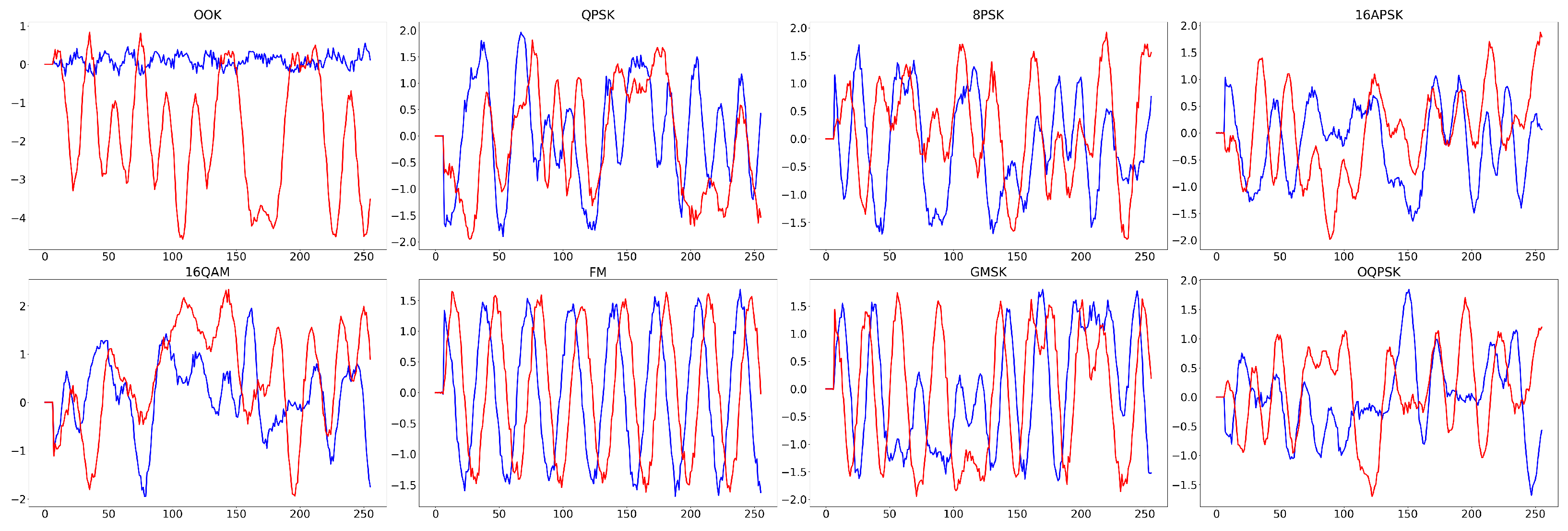
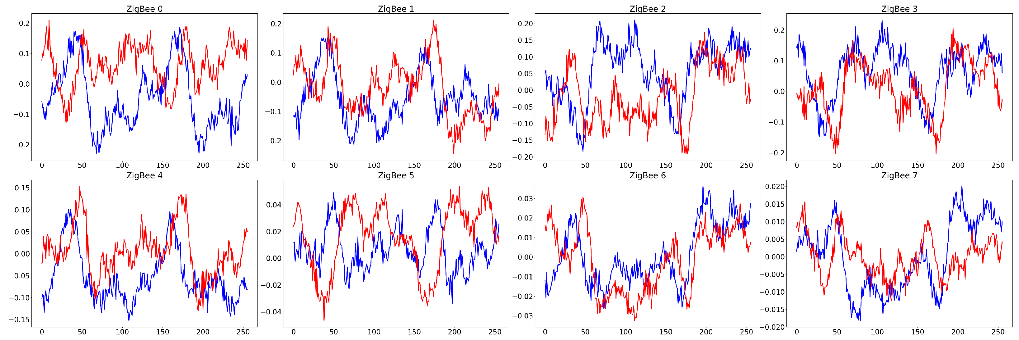
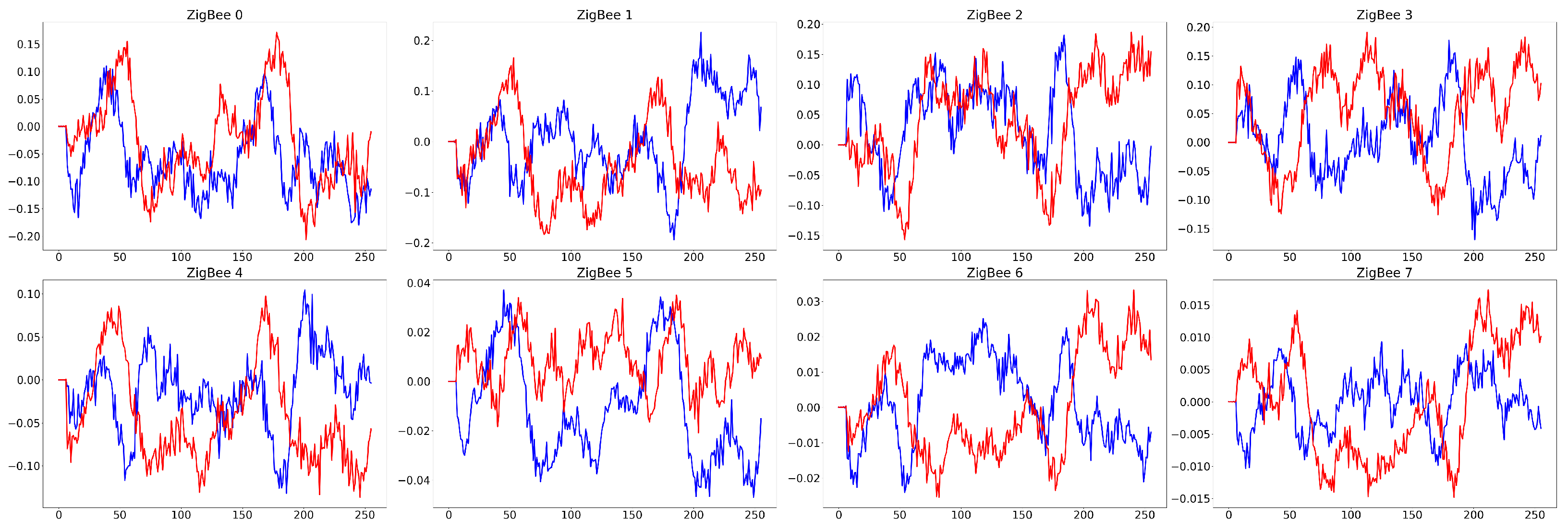
In addition, in order to better solve the problem of the difficulty to collect and label the sample data of the RF signal present in the target domain under the cross-scenario, the sample size of the target domain dataset is only half of that of the source domain, and all RF signal samples in the target domain are unlabeled. The RF signal dataset constructed in this way under the cross-scenario can be used to verify the feasibility of the UDA-based RF signal attribute recognition method.

Table 8. RF signal dataset for the AMR task across G2G→A2G and A2G→G2G scenarios.

Dataset Settings	Ground-to-Ground→Air-to-Ground (G2G→A2G)		Air-to-Ground→Ground-to-Ground (A2G→G2G)
	Source	Target	Source	Target
Sample size	84,480	42,240	84,480	42,240
Percentage with label	100%	0%	100%	0%
Signal dimension	1024 × 2
SNR	−10 dB to 10 dB, with a interval of 2 dB
Training: testing	9:1
Type of modulation	8 modulation types: OOK, QPSK, 8PSK, 16APSK, 16QAM, FM, GMSK, OQPSK

and

Table 9. RF signal dataset for the RFFI task across G2G→A2G and A2G→G2G scenarios.

Dataset Settings	Ground-to-Ground→Air-to-Ground (G2G→A2G)		Air-to-Ground→Ground-to-Ground (A2G→G2G)
	Source	Target	Source	Target
Sample size	38,640	19,320	38,640	19,320
Percentage with label	100%	0%	100%	0%
Signal dimension	1024 × 2
SNR	−20 dB to 20 dB, intervals 2 dB
Training: testing	9:1
Type of ZigBee devices	8 ZigBee devices: 0, 1, 2, 3, 4, 5, 6, 7

show the basic attributes of the RF signal dataset under the two tasks of AMR and RFFI, respectively. Figure 3, Figure 4, Figure 5 and Figure 6 present the time-domain waveform of the G2G and A2G scenarios in these two tasks.

5.1.2. Experimental Setup

The experimental setup is presented across two dimensions: software and hardware. On the software front, the Ubuntu 18.04 operating system is selected, with Python 3.8 serving as the primary programming language for the experiments conducted herein. The deep learning framework of choice is PyTorch, which is integrated with CUDA acceleration libraries to utilize the full computational capabilities of GPUs.

Regarding the hardware configuration, an NVIDIA TITAN XP graphics card with 12 GB of memory and an architecture optimized for parallel computing is used, thereby expediting the model training process. Supplementing this is an Intel Xeon E5-2650 V4 processor and 64 GB RAM, endowing the computing platform with ample computational resources and memory to handle data processing and model training efficiently.

5.1.3. Experimental Performance Evaluation

In the experimental performance evaluation, accuracy serves as the primary metric in this study. In multi-class scenarios, accuracy represents the proportion of samples correctly classified across the entire test set. The formula for calculating the accuracy of RF signal attribute recognition is as follows:

$$\begin{array}{c}\hfill \mathrm{Accuracy}={\displaystyle \frac{1}{N}}\sum _{i=1}^C{n}_i,\end{array}$$

(21)

where $n_i$ denotes the number of correctly recognized samples for the i-th attribute, C is the total number of attribute categories, and N is the total number of samples in the test set. This metric provides an intuitive assessment of the model’s overall performance in recognizing different modulation schemes.

Moreover, we also introduce the t-distributed stochastic neighbor embedding (t-SNE) for visual representation and analysis of results. t-SNE is a nonlinear dimensionality reduction technique that maps high-dimensional data to two or three-dimensional spaces while preserving local relationships between data points. Through t-SNE, one can observe the distribution of outputs from different methods, gaining insight into the cohesion within different emitter categories and the separation between them. This visual analysis aids in understanding the model’s performance in multi-class classification tasks and comparing the merits and demerits of different feature extraction.

5.1.4. Experimental Comparison of Baseline Methods

To compare and highlight the effectiveness of the proposed UDA method, we have set up an experimental framework where the performance of baseline methods is systematically analyzed. In this experimental setup, the results obtained by supervised training on labeled data from the target domain and testing directly within the same domain serve as the lower limit of the baseline comparison. Conversely, the results achieved by training and testing on all available signal data in the target domain, with true labels, represent the upper limit of the baseline comparison. Additionally, this study employs two methods designed to address distribution discrepancies in cross-domain data: LTS-SEI and DANN. The LTS-SEI method is used for unsupervised domain adaptation in RFFI, enhancing cross-scenario performance in RF signal attribute recognition. DANN, a pivotal method in domain adaptation, employs adversarial training to adjust the model to the data feature distribution in new scenarios, effectively overcoming the limitations traditional methods face when dealing with inconsistencies in data distribution between source and target domains. Thus, these four baseline methods provide a comprehensive assessment of the effectiveness and robustness of the UDA method proposed herein, thereby better understanding its potential and limitations in practical applications.

5.1.5. Experimental Settings

Experimental configurations are pivotal in the realm of UDA. The choice of parameter settings during model training significantly influences the learning outcomes. Initially, the balancing factors are crucial for modulating the influence of various loss functions, ensuring seamless model transfer across domains. Specifically, the parameters $\rho$, $\beta$, $\gamma$, and $\eta$ govern the noise perturbation consistency loss, the sample-level maximum correlation loss, the distribution-level maximum similarity loss, the domain adversarial loss, and the classification loss, respectively. Proper tuning of these parameters aids in maintaining the model’s performance stability during different datasets, such as from G2G to A2G and vice versa. Furthermore, the learning rate $lr$ impacts the model’s optimization velocity and convergence quality. An inappropriate learning rate, whether too high or too low, may result in learning process instability or delayed convergence. A comprehensive consideration of these parameters enhances the model’s generalization and adaptability.

Table 10. Experimental configuration for two tasks.

Tasks	Hyperparameters
	$\mathit{\rho }$	$\mathit{\beta }$	$\mathit{\gamma }$	$\mathit{\eta }$	lr
AMR	1.0	0.1	1.0	2.0	$1\times {10}^{-3}$
RFFI					$7\times {10}^{-4}$

provides a comprehensive overview of the specific values for these five critical parameter configurations across the four transfer scenarios examined in the experiments.

5.2. Results and Analysis

5.2.1. Performance Degradation across Various Communication Scenarios

Table 11. Performance degradation of AMR and RFFI tasks across various communication scenarios.

Task		Accuracy (%)
		AMR		RFFI
	Test Scenario	G2G	A2G	G2G	A2G
Train Scenario
G2G		72.9	34.9	95.9	79.3
A2G		53.5	69.3	55.5	94.9

presents the test results for AMR and RFFI tasks within the G2G and A2G channel scenarios, without domain adaptation, where the number of training signal samples is consistent across all scenarios.

In the AMR task, the accuracy for training and testing within the same channel scenario, G2G and A2G, were 72.9% and 69.3%, respectively. However, the model trained in the G2G scenario and tested in the A2G scenario yielded an accuracy of 34.7%, representing a substantial decrease from 69.3% to 34.7%, a relative drop of 49.6%. Similarly, the model trained in the A2G scenario and tested in the G2G scenario achieved an accuracy of 53.5%, indicating a decline from 72.9% to 53.5% or a 26.6% reduction relative to the original accuracy.

In the RFFI task, training and testing within the A2G scenario achieved an accuracy of 94.9%. When the model trained in the G2G scenario was tested in the A2G scenario, the accuracy dropped to 79.3%, a relative decrease of 16.4% from the initial 94.9%. Conversely, training and testing within the G2G scenario resulted in an accuracy of 95.9%. When the model trained in the A2G scenario was tested in the G2G scenario, the accuracy plummeted to 55.5%, indicating a significant performance decline from 95.9% to 55.5% or a 42.1% decrease.

These experimental findings indicate that models trained and tested in different scenarios exhibit varying degrees of performance degradation when tested across scenarios. This decline in performance prevents the practical deployment and application of trained models across different channel scenarios.

5.2.2. Comparison of Unsupervised Domain Adaptation Methods

Table 12. Comparison of UDA methods for cross-scenario RF signal attribute recognition in two tasks.

Method	Accuracy (%)
	AMR		RFFI
	G2G→A2G	A2G→G2G	G2G→A2G	A2G→G2G
Lower limit	34.9	53.5	79.3	55.5
DANN	62.6	68.3	83.8	58.3
LTS-SEI	63.7	70.2	86.7	69.7
PMS-UDA (Ours)	64.0	69.9	89.1	73.8
Upper limit	67.3	70.5	94.0	94.8

The bold numbers represent the optimal results.

showcases the recognition performance of the proposed PMS-UDA and baseline methods in cross-scenario tasks of RF signal attribute recognition for G2G→A2G and A2G→G2G scenarios. The accuracy of the lower limit, representing the results of supervised training on source domain signal data followed by direct testing in the target domain without any knowledge transfer, is used to measure the performance enhancement facilitated by the UDA method. This lower limit corresponds to the results of supervised training on target domain RF signal samples, which are half in number compared to the source domain. As shown in Table 11, compared to not implementing domain adaptation, the PMS-UDA method improved recognition accuracy by 29.1%, 16.4%, 9.8%, and 18.3%, respectively.

Moreover, the accuracy of upper limit in Table 12 indicates the results obtained by directly using target domain signal data for supervised training and testing. This upper limit serves as a benchmark to compare against the performance of the UDA method approximating supervised training results. According to Table 12, the accuracy ratios of the PMS-UDA method in RF signal attribute recognition compared to the upper limit are 95.1%, 99.1%, 94.8%, and 77.8%. Except for the A2G→G2G scenario, the performance of the PMS-UDA method is closely to that of supervised training. This indicates that the PMS-UDA method effectively facilitates the transfer of essential prior knowledge from the source to the target domain.

Table 12 reveals that LTS-SEI outperforms DANN, primarily due to the inclusion of domain classification and cross-entropy loss functions within LTS-SEI. Across the four cross-scenario cases, the PMS-UDA method shows an average improvement of 0.9%, 0.1%, 3.9%, and 9.8% over baseline methods. Thus, the PMS-UDA method exhibits the highest average recognition accuracy among the three UDA methods examined.

Furthermore, Figure 7 demonstrates that compared to the performance prior to the application of the PMS-UDA method, the model exhibits enhanced recognition accuracy under both tasks across various SNRs after applying the PMS-UDA method. This indicates that the PMS-UDA method effectively facilitates the transfer of prior knowledge across scenarios under both high and low SNR conditions.

Consequently, this experiment concludes that the PMS-UDA method effectively achieves prior knowledge transfer across scenarios and closely approximates the performance of supervised training; additionally, it demonstrates superior cross-scenario knowledge transfer capability relative to the baseline methods.

5.2.3. Ablation Study of the Optimization of Loss Functions

Table 13. Ablation study of optimization loss function in G2G→A2G scenario.

Tasks	Accuracy (%)
	PMS-UDA	PMS-UDA w/o NPCL	PMS-UDA w/o SMCL/DMSL	PMS-UDA w/o DAL
AMR	64.0	52.7	51.5	43.6
RFFI	89.1	83.4	80.4	84.4

The bold numbers represent the optimal results.

illustrates the experimental results of an ablation study designed to assess the contribution of each loss function within the proposed PMS-UDA method. When the noise perturbation consistency loss, the sample-level maximum correlation loss, and the distribution-level maximum similarity loss are omitted from the proposed UDA method, the accuracies for AMR are 52.7%, 51.5%, and 43.6%, respectively, representing decreases of 11.3%, 12.5%, and 20.4% from the complete model. The RFFI task exhibits a similar trend; without these loss functions, the accuracies are 83.4%, 80.4%, and 84.4%, with reductions of 5.7%, 8.7%, and 4.7%, respectively. This experiment confirms that these three types of loss functions are pivotal in enabling effective knowledge transfer in the UDA methods.

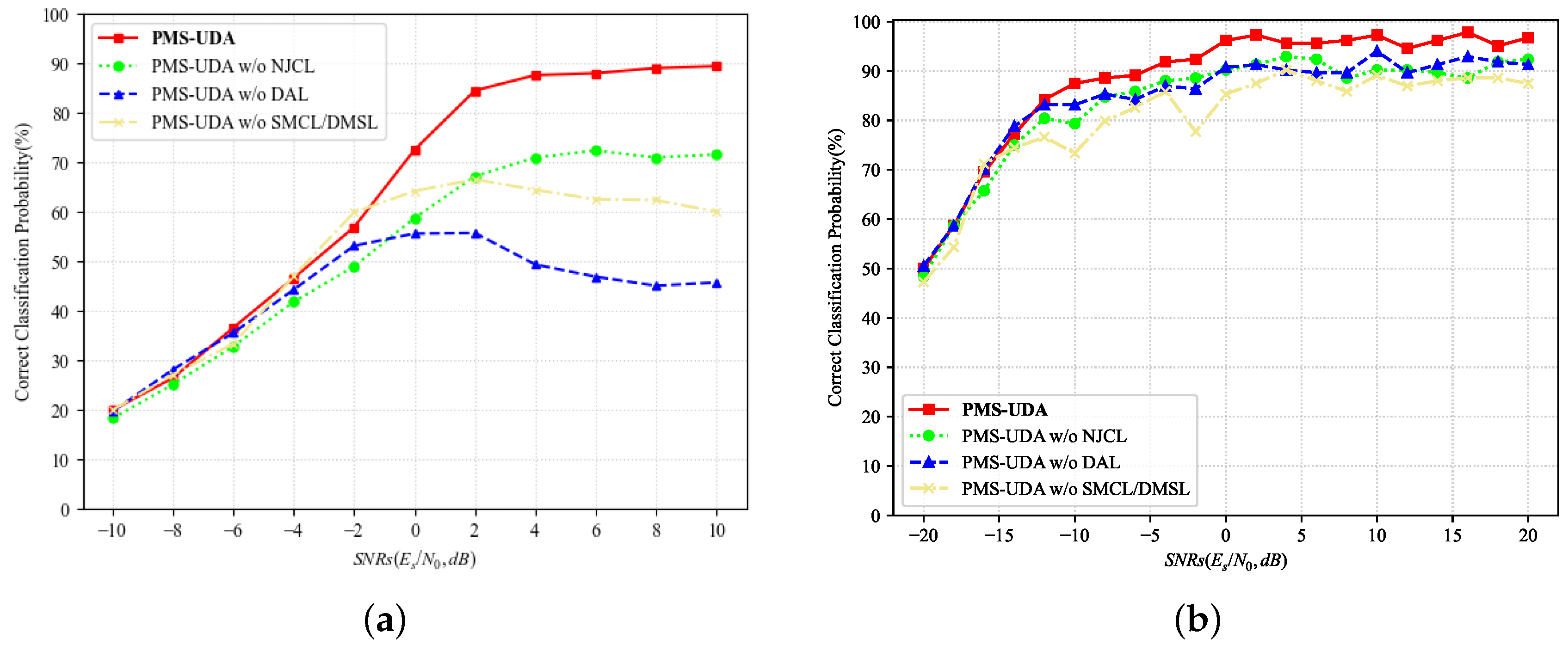
As depicted in Figure 8, the PMS-UDA w/o NPCL method exhibits reduced accuracy at low SNRs, indicating that incorporating noise perturbation consistency learning enhances the method’s robustness against noise in low SNR conditions. This is achieved by introducing random noise perturbation. Conversely, the variant of the PMS-UDA w/o DAL method shows a more pronounced decline in performance at high SNRs. This suggests that domain adversarial learning is instrumental in fostering the acquisition of domain-invariant features across different scenarios at high SNRs, thereby enhancing the representation learning capacity of cross-scenario UDA methods.

Compared to the PMS-UDA method, the performance of PMS-UDA w/o SMCL/DMSL method drops significantly at high SNRs. This underscores the necessity of addressing data distribution discrepancies through optimization at both the sample and distribution levels. Such optimization is essential for minimizing differences in cross-domain data distributions between the source and target domains.

In comparison to the RFFI task, the recognition accuracy of PMS-UDA w/o DAL and PMS-UDA w/o SMCL/DMSL methods in the AMR task demonstrates a decreasing trend with an increase in SNR. A possible reason for this is that the AMR task is more sensitive to the absence of these two losses, particularly at high SNRs. The primary purpose of these losses is to ensure similarity between the feature distributions of the source and target domains, thereby improving the recognition accuracy in the target domain under an unlabeled condition. Without these loss functions, the unsupervised domain adaptation optimization lacks sufficient constraints, which hinders the model’s ability to extract similar and relevant key features, as well as domain-invariant features, ultimately reducing the performance of the PMS-UDA method.

5.2.4. Ablation Study with Progressive Label Alignment Training Methods

Table 14. Ablation study of progressive label alignment training method across scenarios.

Progressive Label Alignment Training Method	Accuracy (%)
	AMR		RFFI
	G2G→A2G	A2G→G2G	G2G→A2G	A2G→G2G
✗	61.3	64.6	83.1	55.0
✓	64.0	69.9	89.1	73.8

The bold numbers represent the optimal results.

presents the accuracies of the proposed PMS-UDA method with or without the employment of the PLAT method, across two tasks in the cross-scenario: G2G to A2G and A2G to G2G. The accuracies of AMR task with PMS-UDA w/o PLAT for two cross-scenarios are 61.3% and 64.6%, respectively. When the PLAT method is employed, the accuracies of the PMS-UDA method improve to 64.0% and 69.9%, reflecting gains of 2.7% and 5.3%, respectively.

In the RFFI task, the performance of the PMS-UDA w/o PLAT method yields accuracies of 83.1% for the G2G→A2G scenario and 53.4% for the A2G to G2G scenario. Upon incorporating the PLAT method, the accuracies of the PMS-UDA method rise to 89.1% and 73.8%, demonstrating significant improvements of 6.0% and 18.8%, respectively. These results underscore the effectiveness of the PLAT method in facilitating domain knowledge transfer for both RF signal attribute recognition tasks in the unsupervised domain adaptation.

5.2.5. Similarity of Feature Distribution via T-SNE Visualization

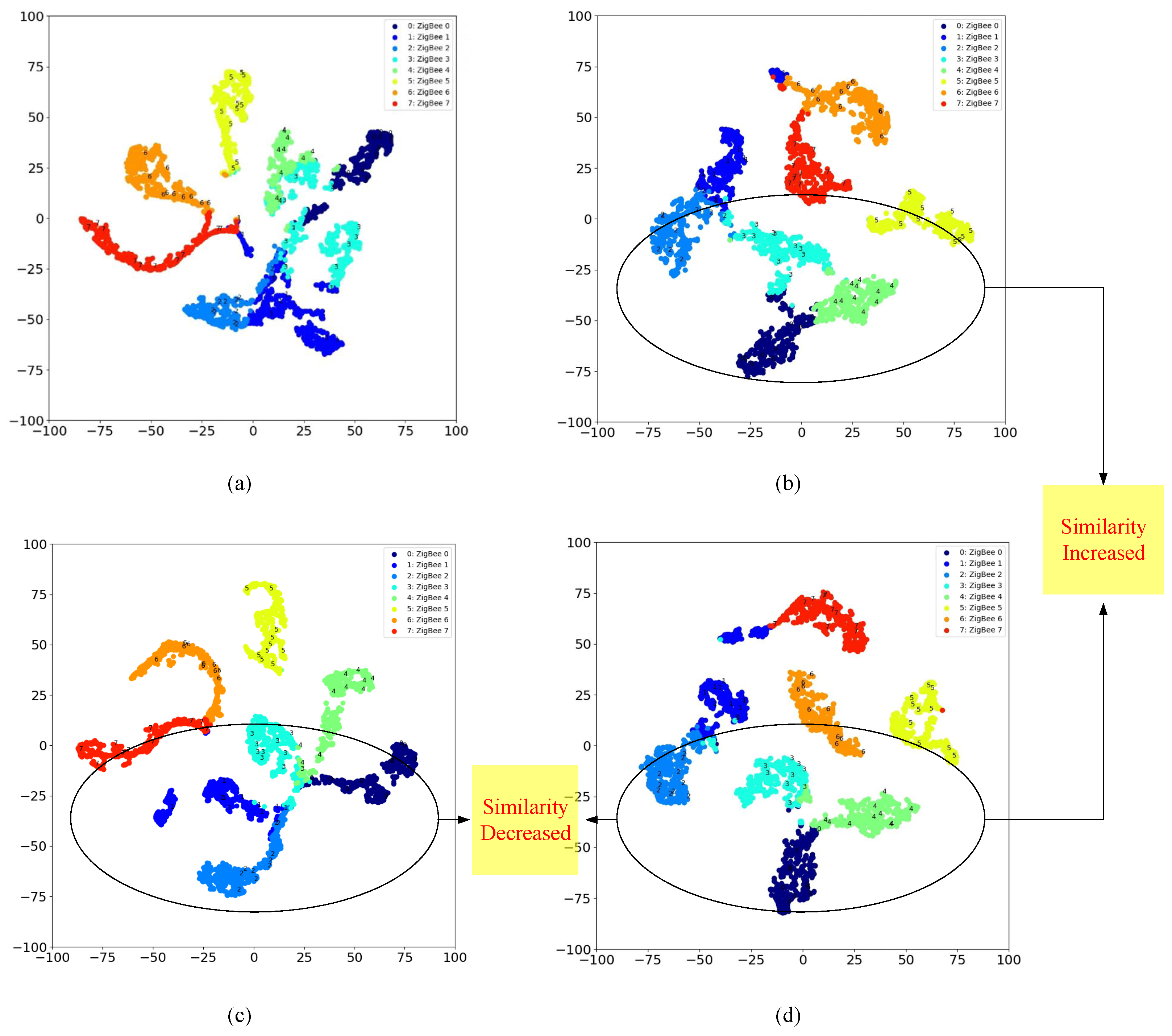
Figure 9 illustrates the experiment designed to showcase the evolution of feature distributions through domain adaptation for the G2G→A2G scenario. Initially, as depicted in Figure 9a,c, there is a noticeable divergence in the feature distribution between the source domain G2G and the target domain A2G. However, following domain adaptation, the scenario changes, as indicated in Figure 9b,d, with an increase in the similarity of the feature distributions between the two domains.

Furthermore, the accuracies for the source domain G2G scenario are observed to be 95.2% before and 95.6% after domain adaptation, as shown in Figure 9c,d. This minor yet significant improvement of 0.4% post-adaptation not only enhances the recognition accuracy but also aligns the feature similarities more closely with those in the target domain. A comparison between Figure 9a,b reveals that the domain adaptation for A2G scenario exhibits greater inter-class dispersion and tighter intra-class distribution compared to their pre-adaptation state.

The conclusions drawn from this experiment suggest that the proposed UDA method is effective in achieving analogous feature distributions across the source and target domains. Additionally, it fosters greater dispersion among classes and tighter cohesion within classes for RFFI in the target domain.

6. Conclusions

In this paper, we propose a PMS-UDA method for RF signal attribute recognition that demonstrates remarkable robustness against noise and maximizes the similarity of signal distribution across communication scenarios. This method effectively enables the model to handle signals across various SNRs by recognizing that samples perturbed by slight noise share the same label. Additionally, our method incorporates sample-level maximum correlation and distribution-level maximum similarity optimization, enhancing the alignment and similarity of feature distribution between the source and target domains. Through domain adversarial learning, the model extracts domain-invariant features, minimizing the impact of differences in channel scenarios. A progressive label alignment training method further refines this process by utilizing pseudo-labels from unlabeled samples in prior phases to achieve maximum sample-level correlation and distribution-level similarity in subsequent phases. The experimental results confirm that our PMS-UDA method approaches the upper limit of the target domain supervised training. It also proves particularly effective under low SNR conditions, affirming its utility in achieving feature distribution similarity between the source and target domains.

References

1. Labib, N.S.; Danoy, G.; Musial, J.; Brust, M.R.; Bouvry, P. A Multilayer Low-Altitude Airspace Model for UAV Traffic Management. In Proceedings of the 9th ACM Symposium on Design and Analysis of Intelligent Vehicular Networks and Applications, DIVANet ’19, Miami Beach, FL, USA, 25–29 November 2019; ACM: New York, NY, USA, 2019; pp. 57–63. [Google Scholar] [CrossRef]
2. Watson, T. Maximizing the Value of America’s Newest Resource, Low-Altitude Airspace: An Economic Analysis of Aerial Trespass and Drones. Indiana Law J. 2020, 95, 1399–1435. [Google Scholar]
3. Zhang, H.; Wang, L.; Tian, T.; Yin, J. A Review of Unmanned Aerial Vehicle Low-Altitude Remote Sensing (UAV-LARS) Use in Agricultural Monitoring in China. Remote Sens. 2021, 13, 1221. [Google Scholar] [CrossRef]
4. Yi, J.; Zhang, H.; Wang, F.; Ning, C.; Liu, H.; Zhong, G. An Operational Capacity Assessment Method for an Urban Low-Altitude Unmanned Aerial Vehicle Logistics Route Network. Drones 2023, 7, 582. [Google Scholar] [CrossRef]
5. Guo, T.; Jiang, N.; Li, B.; Zhu, X.; Wang, Y.; Du, W. UAV Navigation in High Dynamic Environments: A Deep Reinforcement Learning Approach. Chin. J. Aeronaut. 2021, 34, 479–489. [Google Scholar] [CrossRef]
6. Lyu, C.; Zhan, R. Global Analysis of Active Defense Technologies for Unmanned Aerial Vehicle. IEEE Aerosp. Electron. Syst. Mag. 2022, 37, 6–31. [Google Scholar] [CrossRef]
7. Cai, J.; Gan, F.; Cao, X.; Liu, W.; Li, P. Radar Intra–Pulse Signal Modulation Classification with Contrastive Learning. Remote Sens. 2022, 14, 5728. [Google Scholar] [CrossRef]
8. Zhang, J.; Wang, T.; Feng, Z.; Yang, S. Towards the Automatic Modulation Classification with Adaptive Wavelet Network. IEEE Trans. Cogn. Commun. Netw. 2023, 9, 549–563. [Google Scholar] [CrossRef]
9. Paul, A.K.; Tachibana, A.; Hasegawa, T. An Enhanced Available Bandwidth Estimation Technique for an End-to-End Network Path. IEEE Trans. Netw. Serv. Manag. 2016, 13, 768–781. [Google Scholar] [CrossRef]
10. Abdoush, Y.; Pojani, G.; Corazza, G.E. Adaptive Instantaneous Frequency Estimation of Multicomponent Signals Based on Linear Time–Frequency Transforms. IEEE Trans. Signal Process. 2019, 67, 3100–3112. [Google Scholar] [CrossRef]
11. Huang, B.; Lin, C.L.; Chen, W.; Juang, C.F.; Wu, X. Signal Frequency Estimation Based on RNN. In Proceedings of the 2020 Chinese Control And Decision Conference (CCDC), Hefei, China, 22–24 August 2020; pp. 2030–2034. [Google Scholar] [CrossRef]
12. Sun, L.; Ke, D.; Wang, X.; Huang, Z.; Huang, K. Robustness of Deep Learning-Based Specific Emitter Identification under Adversarial Attacks. Remote Sens. 2022, 14, 4996. [Google Scholar] [CrossRef]
13. Zeng, Y.; Gong, Y.; Liu, J.; Lin, S.; Han, Z.; Cao, R.; Huang, K.; Letaief, K.B. Multi-Channel Attentive Feature Fusion for Radio Frequency Fingerprinting. IEEE Trans. Wirel. Commun. 2023, 23, 4243–4254. [Google Scholar] [CrossRef]
14. Qi, X.; Hu, A.; Zhang, Z. Data-and-Channel-Independent Radio Frequency Fingerprint Extraction for LTE-V2X. IEEE Trans. Cogn. Commun. Netw. 2024, 10, 905–919. [Google Scholar] [CrossRef]
15. Qiu, Z.; Chu, X.; Calvo-Ramirez, C.; Briso, C.; Yin, X. Low Altitude UAV Air-to-Ground Channel Measurement and Modeling in Semiurban Environments. Wirel. Commun. Mob. Comput. 2017, 2017, 1587412. [Google Scholar] [CrossRef]
16. Tu, K.; Rodríguez-Piñeiro, J.; Yin, X.; Tian, L. Low Altitude Air-to-Ground Channel Modelling Based on Measurements in a Suburban Environment. In Proceedings of the 2019 11th International Conference on Wireless Communications and Signal Processing (WCSP), Xi’an, China, 23–24 October 2019; pp. 1–6. [Google Scholar] [CrossRef]
17. Srivastava, A.; Prakash, J. Internet of Low-Altitude UAVs (IoLoUA): A Methodical Modeling on Integration of Internet of “Things” with “UAV” Possibilities and Tests. Artif. Intell. Rev. 2023, 56, 2279–2324. [Google Scholar] [CrossRef]
18. Wang, M.; Lin, Y.; Tian, Q.; Si, G. Transfer Learning Promotes 6G Wireless Communications: Recent Advances and Future Challenges. IEEE Trans. Reliab. 2021, 70, 790–807. [Google Scholar] [CrossRef]
19. Liu, C.; Wei, Z.; Ng, D.W.K.; Yuan, J.; Liang, Y.C. Deep Transfer Learning for Signal Detection in Ambient Backscatter Communications. IEEE Trans. Wirel. Commun. 2021, 20, 1624–1638. [Google Scholar] [CrossRef]
20. Wong, L.J.; Michaels, A.J. Transfer Learning for Radio Frequency Machine Learning: A Taxonomy and Survey. Sensors 2022, 22, 1416. [Google Scholar] [CrossRef]
21. Deng, W.; Xu, Q.; Li, S.; Wang, X.; Huang, Z. Cross-Domain Automatic Modulation Classification Using Multimodal Information and Transfer Learning. Remote Sens. 2023, 15, 3886. [Google Scholar] [CrossRef]
22. Jing, Z.; Li, P.; Wu, B.; Yuan, S.; Chen, Y. An Adaptive Focal Loss Function Based on Transfer Learning for Few-Shot Radar Signal Intra-Pulse Modulation Classification. Remote Sens. 2022, 14, 1950. [Google Scholar] [CrossRef]
23. Patel, V.M.; Gopalan, R.; Li, R.; Chellappa, R. Visual Domain Adaptation: A survey of recent advances. IEEE Signal Process. Mag. 2015, 32, 53–69. [Google Scholar] [CrossRef]
24. Wang, M.; Deng, W. Deep Visual Domain Adaptation: A Survey. Neurocomputing 2018, 312, 135–153. [Google Scholar] [CrossRef]
25. Wilson, G.; Cook, D. A Survey of Unsupervised Deep Domain Adaptation. ACM Trans. Intell. Syst. Technol. 2020, 11, 1–46. [Google Scholar] [CrossRef] [PubMed]
26. Farahani, A.; Voghoei, S.; Rasheed, K.; Arabnia, H.R. A Brief Review of Domain Adaptation. In Advances in Data Science and Information Engineering; Transactions on Computational Science and Computational Intelligence; Springer: Cham, Switzerland, 2021. [Google Scholar]
27. Bu, K.; He, Y.; Jing, X.; Han, J. Adversarial transfer learning for deep learning based automatic modulation classification. IEEE Signal Process. Lett. 2020, 27, 880–884. [Google Scholar] [CrossRef]
28. Liu, P.; Guo, L.; Zhao, H.; Shang, P.; Chu, Z.; Lu, X. A Long Time Span-Specific Emitter Identification Method Based on Unsupervised Domain Adaptation. Remote Sens. 2023, 15, 5214. [Google Scholar] [CrossRef]
29. Xiao, J.; Wang, Y.; Zhang, D.; Ma, Q.; Ding, W. Multiscale Correlation Networks Based On Deep Learning for Automatic Modulation Classification. IEEE Signal Process. Lett. 2023, 30, 633–637. [Google Scholar] [CrossRef]
30. Xiao, J.; Ding, W.; Shao, Z.; Zhang, D.; Ma, Y.; Wang, Y.; Wang, J. Multi-Periodicity Dependency Transformer Based on Spectrum Offset for Radio Frequency Fingerprint Identification. arXiv 2024, arXiv:2408.07592. [Google Scholar] [CrossRef]
31. Endres, D.M.; Schindelin, J.E. A new metric for probability distributions. IEEE Trans. Inf. Theory 2003, 49, 1858–1860. [Google Scholar] [CrossRef]
32. Kullback, S.; Leibler, R.A. On Information and Sufficiency. Ann. Math. Stat. 1951, 22, 79–86. [Google Scholar] [CrossRef]
33. Tu, Y.; Lin, Y.; Zha, H.; Zhang, J.; Wang, Y.; Gui, G.; Mao, S. Large-Scale Real-World Radio Signal Recognition with Deep Learning. Chin. J. Aeronaut. 2022, 35, 35–48. [Google Scholar] [CrossRef]
34. Matolak, D.W.; Sun, R. Air–ground channel characterization for unmanned aircraft systems—Part III: The suburban and near-urban environments. IEEE Trans. Veh. Technol. 2017, 66, 6607–6618. [Google Scholar] [CrossRef]
35. O’Shea, T.J.; Roy, T.; Clancy, T.C. Over-the-Air Deep Learning Based Radio Signal Classification. IEEE J. Sel. Top. Signal Process. 2018, 12, 168–179. [Google Scholar] [CrossRef]
Figure 1. Optimization method for cross-scenario RF signal attribute recognition.
Remotesensing 16 03696 g001
Figure 2. Illustrative diagrams of RF signal dataset in the air-to-ground channel scenario.
Remotesensing 16 03696 g002
Figure 3. Time-domain waveforms of various modulated signals for G2G channel scenarios at SNR = 10 dB. The red and blue curves represent the in-phase (I) and quadrature (Q) components, respectively.
Remotesensing 16 03696 g003
Figure 4. Time-domain waveforms of various modulated signals for A2G channel scenario at SNR = 10 dB.
Remotesensing 16 03696 g004
Figure 5. Time-domain waveform of ZigBee signals for G2G channel scenario at SNR = 10 dB.
Remotesensing 16 03696 g005
Figure 6. Time-domain waveform of ZigBee signals for A2G channel scenario at SNR = 10 dB.
Remotesensing 16 03696 g006
Figure 7. Comparison of the performance before and after using PMS-UDA method. (a) AMR Task. (b) RFFI Task.
Remotesensing 16 03696 g007
Figure 8. Ablation study of the optimization of loss function in the G2G→A2G scenario. (a) AMR Task. (b) RFFI Task.
Remotesensing 16 03696 g008
Figure 9. Feature distribution of ZigBee signal before and after UDA across G2G→A2G scenario. (a) A2G signal feature distribution before UDA. (b) A2G signal feature distribution after UDA. (c) G2G signal feature distribution before UDA. (d) G2G signal feature distribution after UDA.
Remotesensing 16 03696 g009