Article

A 40-Year Time Series of Land Surface Emissivity Derived from AVHRR Sensors: A Fennoscandian Perspective

1
Institute of Geography, University of Bern, Hallerstr. 12, 3012 Bern, Switzerland
2
Oeschger Centre for Climate Change Research, University of Bern, Hochschulstr. 4, 3012 Bern, Switzerland
*
Author to whom correspondence should be addressed.
Remote Sens. 2024, 16(19), 3686; https://doi.org/10.3390/rs16193686
Submission received: 12 August 2024 / Revised: 14 September 2024 / Accepted: 27 September 2024 / Published: 2 October 2024

Abstract

:
Accurate land surface temperature (LST) retrieval depends on precise knowledge of the land surface emissivity (LSE). Neglecting or inaccurately estimating the emissivity introduces substantial errors and uncertainty in LST measurements. The emissivity, which varies across different surfaces and land uses, reflects material composition and surface roughness. Satellite data offer a robust means to determine LSE at large scales. This study utilises the Normalised Difference Vegetation Index Threshold Method (NDVITHM) to produce a novel emissivity dataset spanning the last 40 years, specifically tailored for the Fennoscandian region, including Norway, Sweden, and Finland. Leveraging the long and continuous data series from the Advanced Very High Resolution Radiometer (AVHRR) sensors aboard the NOAA and MetOp satellites, an emissivity dataset is generated for 1981–2022. This dataset incorporates snow-cover information, enabling the creation of annual emissivity time series that account for winter conditions. LSE time series were extracted for six 15 × 15 km study sites and compared against the Moderate Resolution Imaging Spectroradiometer (MODIS) MOD11A2 LSE product. The intercomparison reveals that, while both datasets generally align, significant seasonal differences exist. These disparities are attributable to differences in spectral response functions and temporal resolutions, as well as the method considering fixed values employed to calculate the emissivity. This study presents, for the first time, a 40-year time series of the emissivity for AVHRR channels 4 and 5 in Fennoscandia, highlighting the seasonal variability, land-cover influences, and wavelength-dependent emissivity differences. This dataset provides a valuable resource for future research on long-term land surface temperature and emissivity (LST&E) trends, as well as land-cover changes in the region, particularly with the use of Sentinel-3 data and upcoming missions such as EUMETSAT’s MetOp Second Generation, scheduled for launch in 2025.

Graphical Abstract

1. Introduction

Land surface temperature (LST) is a key variable in land surface energy balance models. It represents the land–atmosphere interaction and has been widely used for climate change research [1,2,3]. LST was identified by the Global Climate Observing System (GCOS) as an Essential Climate Variable (ECV) in 2016 [4]. The GCOS sets requirements for ECV products that are expressed in terms of different criteria, such as temporal and spatial resolution, measurement uncertainty, and stability. The required measurement uncertainty for LST should be below 1 K [5]. Satellite LST data are retrieved from brightness temperatures measured in the thermal infrared (TIR) portion of the electromagnetic spectrum between 8 and 14 µm [6]. The determination of LST from satellites is an ill-posed problem, as the radiance emitted from the surface in the IR region is a function of its temperature and emissivity [7]. LST retrievals relying on split-window algorithms, which exploit differential absorption in two spectrally close TIR window channels for atmospheric correction, require a priori knowledge of the land surface emissivity (LSE) [8,9]. A multi-channel approach can be used for satellite sensors with more than two TIR bands to retrieve LST and LSE simultaneously. For two channels, LSE is determined from auxiliary data. Therefore, LSE variability directly affects the LST uncertainty budget [10].
LSE is an intrinsic property of the surface and varies with surface composition, such as soil moisture, roughness, and particle size [11]. It is a measure of the efficiency with which surfaces convert kinetic into radiant energy. LSE is a major source of uncertainty when retrieving LST, and if neglected, it can lead to substantial errors in the LST product. In moderate environmental conditions, a 1% uncertainty in the prediction accuracy of LSE can result in a temperature retrieval error of around 0.5 K, introducing a systematic error in the entire temperature product [12]. However, these estimates are difficult to compute and generalise. For example, Schädlich et al. [13] indicated an LST error of ±2 K for an emissivity error of ±0.025, and Sobrino et al. [14] stated that LSE should have an accuracy of ±0.005 to keep the temperature error below 0.4 K. Generally, the temperature error increases with lower emissivities and is smallest for emissivity values close to 1. According to Becker [15], the error in LST, symbolised by Δ T, can be expressed as
Δ T = 50 1 ε ε 300 Δ ε ε
where ε represents the mean channel emissivity and Δ ε represents the emissivity difference of two adjacent TIR channels. Considering the Advanced Very High Resolution Radiometer (AVHRR) channels 4 and 5 emissivities ( ε c h 4 and ε c h 5 , respectively),
ε = ε c h 4 + ε c h 5 2 and Δ ε = ε c h 4 ε c h 5
High-latitude regions are experiencing rapid warming, resulting in significant reductions in snow and ice cover, thawing permafrost, increased vegetation productivity, and fluvial and coastal erosion [16,17]. Arctic warming is driving shifts in vegetation patterns [18]; for example, an increase in the shrub distribution has been observed in high-latitude regions [19]. Fennoscandia, encompassing Finland and the Scandinavian Peninsula, is characterised by a high mountain range in the west and tundra in the north [20], supporting a wide range of vegetation types. Climate simulations from Lagergren et al. [21] suggest that changes in vegetation patterns driven by climate change will have a profound impact on forestry, tourism, and reindeer herding, as well as severe consequences for rare and endangered species. Arctic warming is also accelerating permafrost degradation and increasing the frequency of extreme weather events, potentially leading to tundra browning [22].
LST and LSE data are a good proxy for land-cover changes in the terrestrial biosphere [23]. In this regard, an emissivity dataset for Fennoscandia between 1981 and 2022, based on the AVHRR LAC archive stored at the University of Bern (as described in [24]), has been developed. LSE can be obtained using different methods [25,26], and the optimal approach is dictated by the spatial, temporal, and spectral resolution of the considered sensor. To utilise the entire AVHRR archive, the Normalised Difference Vegetation Index Threshold Method (NDVITHM) [27,28], based on AVHRR channels 1 and 2, is chosen, as data from these two bands have been available since the launch of the first sensor. In remote sensing, the Normalised Difference Vegetation Index (NDVI) is used as an indicator of vegetation health and coverage. The index is calculated with the spectral reflectance in the near-infrared (NIR) and visible red (R) wavelengths: NDVI = (NIR − Red)/(NIR + Red). The value lies between −1 and 1, with positive values close to 1 indicating full coverage of healthy vegetation. Negative values indicate water bodies, rocks, or artificial surfaces like concrete and thus represent the absence of vegetation [29].
Emissivity maps derived from Meteosat Second Generation (MSG)’s Spinning Enhanced Visible and InfraRed Imager (SEVIRI), the Advanced Spaceborne Thermal Emission and Reflection Radiometer (ASTER), or the Moderate Resolution Imaging Spectroradiometer (MODIS) cover Fennoscandia, or parts of it, for certain periods [2,25,30]. However, no emissivity datasets cover northern Europe for the 1981–2022 period. To retrieve statistically significant changes in ECVs, such as LST, a time series of at least 30 years is required [31]. Only the data from the Advanced Very High Resolution Radiometer (AVHRR) sensors onboard the NOAA and MetOp satellite series provide data covering more than four decades. Furthermore, most existing LSE products rely on static land-cover data, which present severe deficiencies in the high northern latitudes, primarily due to an inaccurate representation of wetlands [16]. This study addresses this gap by developing a comprehensive 40-year Fennoscandian emissivity dataset for the AVHRR 10.8 and 11.5 µm channels, accounting for seasonal emissivity changes independently of land-cover classifications.

Land Surface Emissivity

The LSE ( ϵ ) is a proportionality factor that scales blackbody radiance (Planck’s law) to predict emitted radiance and represents the efficiency of transmitting thermal energy across the surface into the atmosphere [7,32,33]. Per the definition, the emissivity of a blackbody is 1.0. Natural objects, on the other hand, are imperfect emitters and emit radiation based on their emissivity, which varies with wavelength and depends on the material composition and surface temperature of the object. The spectral emissivity of a non-blackbody M λ in relation to a blackbody M λ S as a function of temperature (T) and wavelength ( λ ) [33,34,35] can thus be expressed as
ε λ ( T ) = M λ ( λ , T ) M λ S ( λ , T )
The emissivity of the land surface depends on the type of surface cover, its composition and roughness, and the distribution and density of vegetation, as well as the structure, moisture content, and organic composition of the soils [36,37]. Changes in surface emissivity for most natural surfaces occur primarily due to variations in soil moisture, mineralogy, vegetation cover, snow and ice cover, and surface roughness [2].
In areas with full vegetation, the emissivity is relatively consistent and close to a value of 1.0 in the thermal infrared region (e.g., Van de Griend and Owe [38] suggest a range of 0.95–1). In contrast, urban land and dry areas with scarce vegetation have more complex emissivity patterns ranging from 0.40 to 0.98 [36,39]. Snow generally has a high emissivity of 0.985–0.990, with minor variations caused by the density and water content of the snow, as well as grain shape and size (surface roughness) [40].
Figure 1 presents the emissivity spectra for key land-cover classes relevant to this study, derived from the ECOSTRESS spectral library [41,42]. As detailed above, even small variations in emissivity can significantly influence land surface temperature (LST). To account for wavelength-dependent emissivity differences, the dataset produced in this study specifically calculates the emissivity for AVHRR channels 4 and 5, centred at 10.8 µm and 11.5 µm, respectively. Notably, soil exhibits lower emissivity in channel 4 compared to channel 5, while forest emissivity (both deciduous and coniferous) remains relatively constant across these wavelengths. In contrast, water and snow (here, medium-granular snow) exhibit a higher emissivity at 10.8 µm than at 11.5 µm. These observations highlight the importance of generating a long-term emissivity time series for Fennoscandia to capture the shifts and variability driven by rising air temperatures, which affect snow-cover duration and vegetation dynamics.

2. Materials and Methods

2.1. Study Area

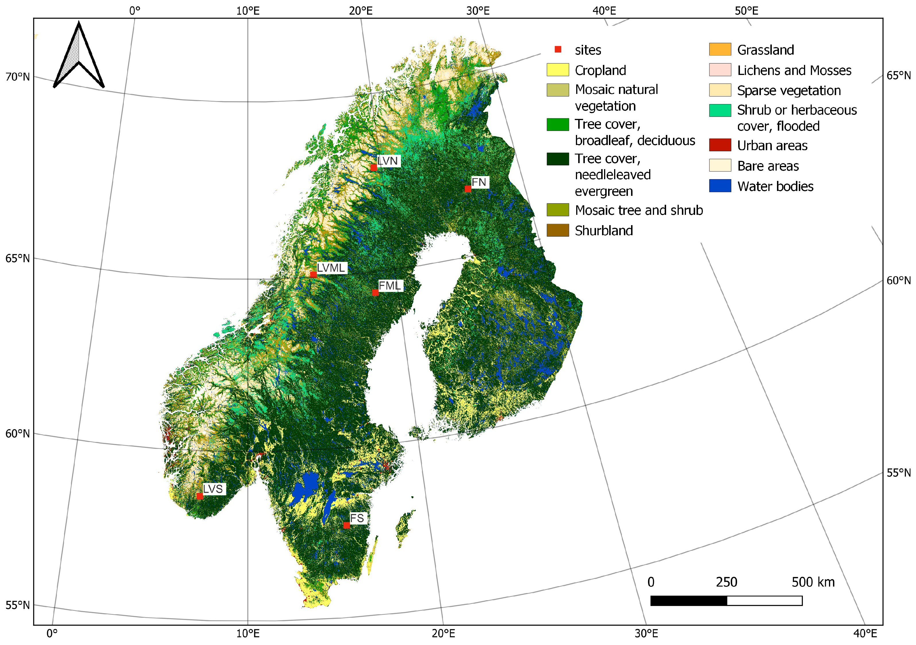
Six zones of interest of approximately 15 × 15 km each in Fennoscandia are chosen for detailed analysis (Figure 2 and Table 1). The determining factors include latitude, land-cover class, and land-cover homogeneity in the 225 km2 areas. To assess the effects of land cover on emissivity, the study sites are chosen to represent two different vegetation categories: forest and low vegetation. To evaluate the impact of latitude and sun zenith angle, the study sites are spread across the southern, mid-latitude, and northern regions. The land-cover dataset used to determine the study sites is the 2015 ESA CCI Land-Cover Dataset at a spatial resolution of 300 m [43].

2.2. AVHRR LAC L1C Data

The AVHRR is the longest-running sensor providing multispectral data, making it invaluable for advanced retrievals of ECVs, such as LST. Since 1978, the AVHRR has delivered daily images across Europe with a medium spatial resolution of approximately 1.1 × 1.1 km at nadir. For this study, we used the AVHRR data archive from the University of Bern [24,44], which contains data from 1981 onward. Data from the first AVHRR-equipped satellite, TIROS-N (in orbit from 1978 to 1981), are excluded from the dataset due to quality and processing limitations [45].
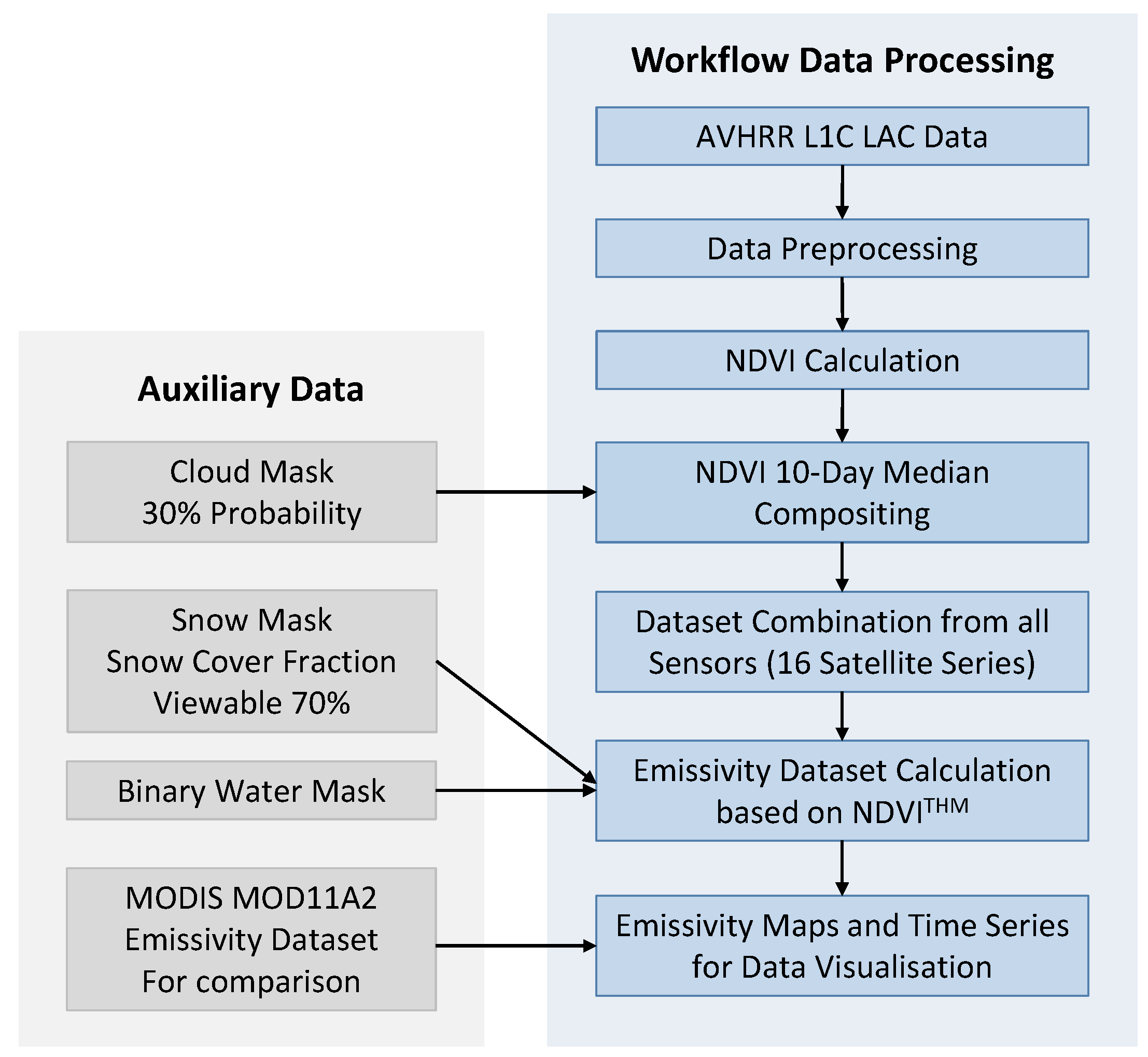
The archived AVHRR swath-based data in Level-1b format are pre-processed for further applications. The pre-processing includes an orthorectification that applies the SAPS (Science Systems and Applications, Inc. AVHRR Processing System [46]) procedure which is based on the work of Khlopenkov et al. [47]. These methods enable achieving a general geometric accuracy of 0.1–0.4 pixels, fulfilling the EUMETSAT and GCOS specifications of 1 km and 1/3 pixel, respectively [48,49]. Further data pre-processing steps include the calibration of the visible channels with the latest PATMOS-X parameters ([50], update 2017) and thermal calibration provided by Kidwell et al. [51,52]. Thus, the historic AVHRR record allows for the investigation of long-term climatological changes and the study of climate variability, fulfilling World Meteorological Organization (WMO) requirements [31]. In Figure 3, the steps of data pre-processing, emissivity calculation, and incorporation of auxiliary datasets are visualised.

2.3. MODIS MOD11A2 Data

The MODIS MOD11A2 LST&E version 6.1 product, recorded from the Terra satellite series, is used for comparison. This is a Level-3 product with a spatial resolution of 1 km at nadir that has provided an average 8-day per-pixel LST and LSE since 2000 [30]. The MOD11A2 8-day composite is computed from all the corresponding MOD11A1 daily values. The emissivities of MOD11A2 bands 31 and 32 are based on land-cover classification and dynamic and seasonal factors, such as vegetation senescence and snow cover [53]. Laboratory-measured emissivity is assigned to the fourteen emissivity classes defined by land cover. MODIS products of land cover, snow, and vegetation index are used to infer the effective emissivities of land surface pixels for the channels.

2.4. NDVI 10-Day MED Composites

To generate LSE maps, 10-day NDVI median value composites (MEDs) are first produced. During the composite calculation, a cloud mask is incorporated to filter out pixels with a probability of at least 30% of containing clouds (NWC-SAF/PPS probabilistic cloud mask (PPS2021-alpha) [54]).
The three generations of AVHRR sensors (AVHRR/1, AVHRR/2, and AVHRR/3) exhibit slightly different spectral response functions (SRFs) [55]. To account for these differences, the NDVI values are normalised to the NOAA-9 NDVI using the correction values proposed by Trishchenko et al. [56,57]. These correction functions have previously been shown to significantly improve the consistency between the NDVIs from various AVHRR sensors [55]. MetOp-3 is excluded from the dataset because the spectral response function correction was unavailable.
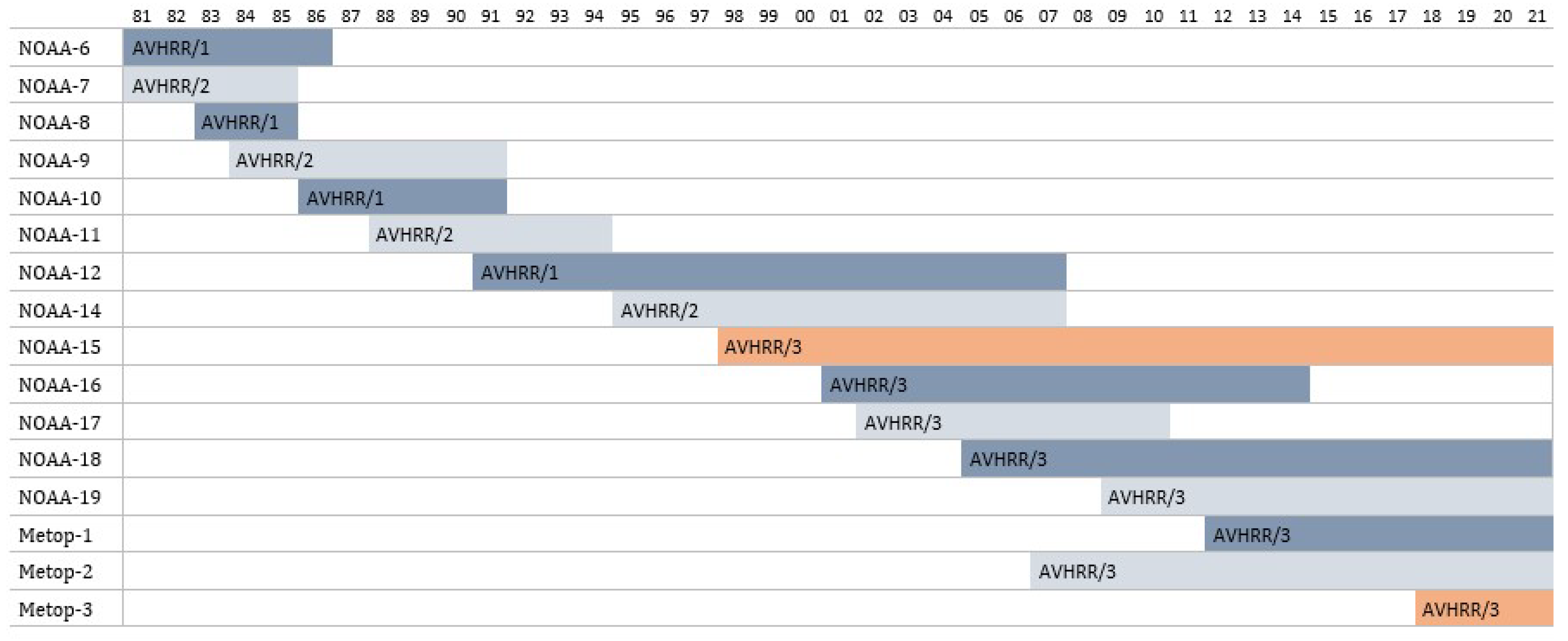
The MEDs are then combined across the different sensors by calculating the median NDVI value for each image pixel across all composite images with the same date (as multiple images from the same date exist due to simultaneously operating sensors, as shown in Figure 4). This process ensures that only one composite image per date is produced. Data from NOAA-15 are excluded from this combination due to frequent errors and missing scan lines throughout the measuring period [58]. Through these processing steps, a consecutive 40-year 10-day MED NDVI dataset is created [59].

2.5. Emissivity Retrieval

A variety of different LSE estimation methods from space exist. Li et al. [7] grouped these methods into three classes: semi-empirical methods (SEMs), such as the classification-based emissivity method (CBEM) and the NDVI-based emissivity method (NBEM), which, in contrast to the NDVITHM, use the correlation between LSE and the logarithm of the NDVI; multi-channel Temperature Emissivity Separation (TES) methods, which retrieve LSE directly from the radiance; and physically based methods (PBMs), which include the TISI-based method, the physics-based day/night operational (D/N) method, and the two-step physical retrieval method (TSRM). There is no single best method for LSE estimation, and depending on the specific application, study goals, and available satellite and sensor specificities, the most appropriate method should be selected.
In this study, an NDVI-based approach was applied to the AVHRR LAC L1C data archive from 1981 to 2022 to produce a 40-year LSE dataset. The NDVI-based method relies on data from AVHRR channels 1 and 2, which have been available since the launch of the first sensor. Other methods to retrieve LSE that would be applicable to AVHRR data, such as the TISI-based or D/N methods, are dependent on channel 3, which has a poor signal-to-noise ratio in the earlier years of AVHRR operation [28]. The widely used TES algorithm cannot be applied to AVHRR data, as it needs at least four different bands in the thermal infrared region, whereas the AVHRR only has two (channels 4 and 5) [26].
Disadvantages and challenges of NDVI-based emissivity methods include the need for a priori knowledge of soil and vegetation emissivities, the accurate definition of NDVI thresholds to distinguish between soil and vegetation, and the accurate estimation of the proportion of the area occupied by vegetation and the vegetation structure to effectively incorporate cavity effects. Further, NDVI-based methods might inaccurately record senescent vegetation and are not applicable to non-vegetated areas like desert areas, bare rock surfaces, water bodies, ice, and snow.

2.5.1. NDVI Threshold Method

The NDVI Threshold Method (NDVITHM), as proposed by Sobrino et al. [28], was selected for this study because it effectively overcomes several of the limitations mentioned in the previous section. For instance, it includes precise estimations of the proportion of the area occupied by vegetation, accounts for cavity effects, and uses experimental emissivity values for soil and vegetation that are adjusted to the specific channel wavelengths.
Sobrino and Raissouni formulated a set of equations for calculating LSE using the NDVI [27]. The basis of the threshold method is a differentiation between vegetated pixels, bare soil pixels, and mixed pixels, followed by a subsequent assignment of the corresponding emissivity values. Generally, pixels with an NDVI lower than 0.2 can be considered bare soil, while an NDVI of 0.5 or higher indicates full vegetation. For pixels with NDVI values between 0.2 and 0.5, it can be assumed that the land is more sparsely vegetated (a mixture of bare soil and vegetation). The proportion of the area occupied by vegetation Pv (also called the fractional vegetation cover) is an important parameter for quantifying the proportion of an area covered by vegetation. This parameter is used to derive the emissivity of mixed pixels, where the NDVI lies between 0.2 and 0.5, and is calculated using the following equation:
P v = ( N D V I N D V I min ) 2 ( N D V I max N D V I min ) 2
The vegetation threshold for Fennoscandia was set to 0.475 to account for lower NDVI values in the high northern latitudes. This threshold correctly classified healthy and dense vegetation for all study sites across Fennoscandia. The threshold of 0.2 for soil accurately classified the pixels and was kept as such. So, for Equation (4), NDVImin = 0.2 for bare soil and NDVImax = 0.475 for full vegetation. For bare soil pixels (NDVI < 0.2), the emissivity values were set to ε s4= 0.95 and ε s5 = 0.96 for channels 4 and 5, respectively, using the experimental values published by Sobrino et al. [28].
In vegetated areas, cavity effects must be considered to avoid underestimating the emissivity. To quantify these effects, a factor (Ci) that incorporates the geometrical differences of natural surfaces, which depend on the vegetation structure and internal reflections, was added to the emissivity value. For flat and homogeneous surfaces Ci ≈ 0. Generally, cavity effects (radiation trapping, multiple scattering, large leaf absorptance) lead to higher emissivities for full vegetation compared to a single leaf, so in most cases, LSE increases with increased vegetation. However, cavity effects are not constant or proportional to the amount of vegetation; especially for intermediate or sparse vegetation cover, these effects should be considered to avoid underestimating the emissivity [60]. According to the geometrical model by Sobrino et al. [61], the values can be approximated as 0.014–0.010 Pv for Ch4 and 0.018–0.014 Pv for Ch5 [28]. For fully vegetated pixels where the NDVI is >0.475 (Pv = 1), ϵ v4 = ϵ v5 = 0.985 was chosen based on the experimental values from Sobrino et al. [28]. Consequently, the mean effective emissivity was formulated with Ci = 0.004 for vegetation:
ϵ v = ϵ 4 = ϵ 5 = 0.985 + C i
To calculate the emissivity for mixed areas with the proportion of vegetated to bare soil areas, the following equation can be used:
ϵ m i = ϵ v i P v + ϵ s i ( 1 P v ) + C i ( i = 4 or 5 )
where ϵvi is the emissivity of vegetation and ϵsi is the emissivity for bare soil for AVHRR channel i (4 or 5).

2.5.2. Dataset Generation

Between 1981 and 2022, 16 different satellites from the NOAA and MetOp series, equipped with AVHRR sensors, were in orbit (Figure 4). The overlapping datasets from these satellites need to be merged to create a single, consistent time series for analysis.
The emissivities were calculated based on the 10-day median NDVI composites to achieve a consistent LSE time series. For each pixel, the emissivity was determined using the NDVITHM defined in Section 2.5.1 and Equations (5) and (6). Pixels with NDVI values below 0.2 were categorised as bare soil, while those above 0.475 were classified as vegetation. The NDVITHM cannot distinguish between bare soil, snow, and water, as these land covers exhibit similarly low NDVI values, leading to potential misclassification. Snow and water both have high average emissivities (around 0.98–0.99 [23,62]) but low NDVI values (snow: −0.1 to 0.1; water: −0.42 to −0.33 [63]), which may lead to these pixels being incorrectly classified as bare soil, resulting in the assignment of emissivity values of 0.95 for channel 4 and 0.96 for channel 5.
To address this issue, snow and water data were integrated to identify these pixels and accurately assign the correct emissivity values. The AVHRR LAC fractional snow-cover product Level 2 developed at the University of Bern was used to identify snow-covered areas [64]. Pixels where the snow-cover fraction viewable (SCFV) was at least 70% were identified as snow. These pixels were then assigned emissivity values of ε snow4 = 0.989 and ε snow5 = 0.982. A binary water mask was derived from the ESA CCI land-cover dataset, with water pixels assigned emissivity values of ε water4 = 0.991 and ε water5 = 0.987, based on laboratory emissivity spectra values of water [23]. To reduce inherent noise and remove outliers, the mean emissivity was computed by averaging the emissivity values across the 15 × 15 km study site at each time step [65].

3. Results

3.1. The 40-Year Time Series

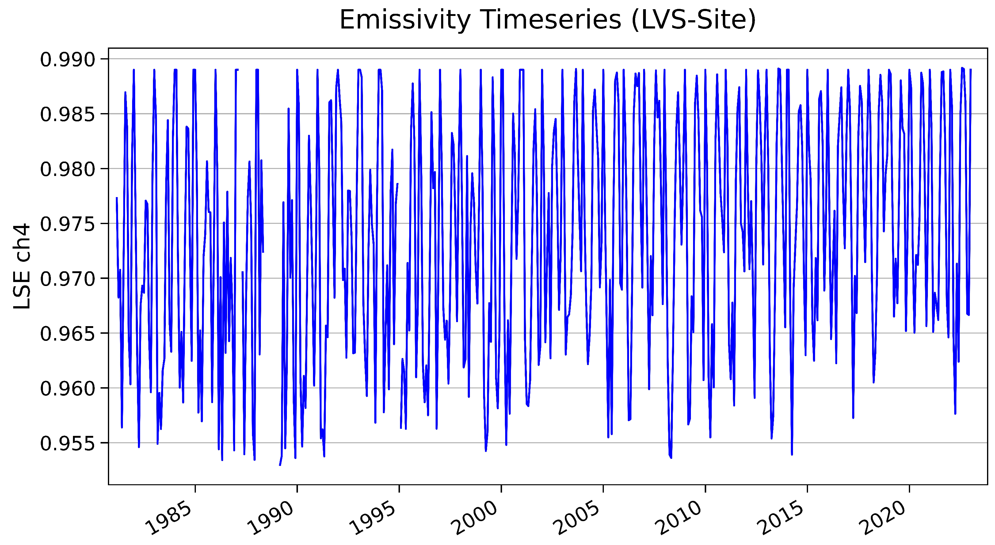
The produced dataset covering Fennoscandia contains land surface emissivities at a spatial resolution of 1.1 km and a temporal resolution of 10 days from 1981 to 2022. Time series were extracted for the six study sites (Figure 2). Figure 5 exhibits the mean emissivity value for the southern low-vegetation site. A strong periodicity is visible in the time series. This phenomenon can be attributed to the high emissivity values of snow and healthy, dense vegetation during summer, and the low emissivity values for melt-out surfaces. The monthly mean, minimum, and maximum NDVI values over the 40-year period for the two southern study sites are listed in Table 2 for both land-cover types—forest (FS) and low vegetation (LVS). Table 2 shows the seasonal variations in the NDVI values for the two different land-cover types. Low NDVI values can be attributed to snow cover or the presence of water, which can directly translate to high emissivity values during the winter. The FS site is characterised by evergreen needle-leaved forest, which explains why high NDVI values were obtained earlier in the year at the FS site than at the LVS site. Negative NDVI values are also present for a longer period at the LVS site.
The monthly mean emissivity values for channels 4 and 5 over the 40-year period for the two southern study sites were calculated to highlight the seasonal emissivity changes and the differences between land-cover types (forest (FS) and low vegetation (LVS)) and latitudes (southern region (S) and northern region (N)) (Table 3). The mean annual cycle over the whole period of interest for the LVS study site is shown in Figure 6. The difference Δ ϵ ( ϵ ch5 ϵ ch4) was used to quantify the disparity between effective emissivities of both channels. A general relation −0.007 ≤ Δ ϵ ≤ 0.01 held for all months and sites. Negative differences in channel emissivity occurred in the presence of snow cover, as the emissivity of snow for channel 4 is higher than that of channel 5 [23]. The smallest absolute differences were mostly experienced in summer when vegetation is dense and healthy.
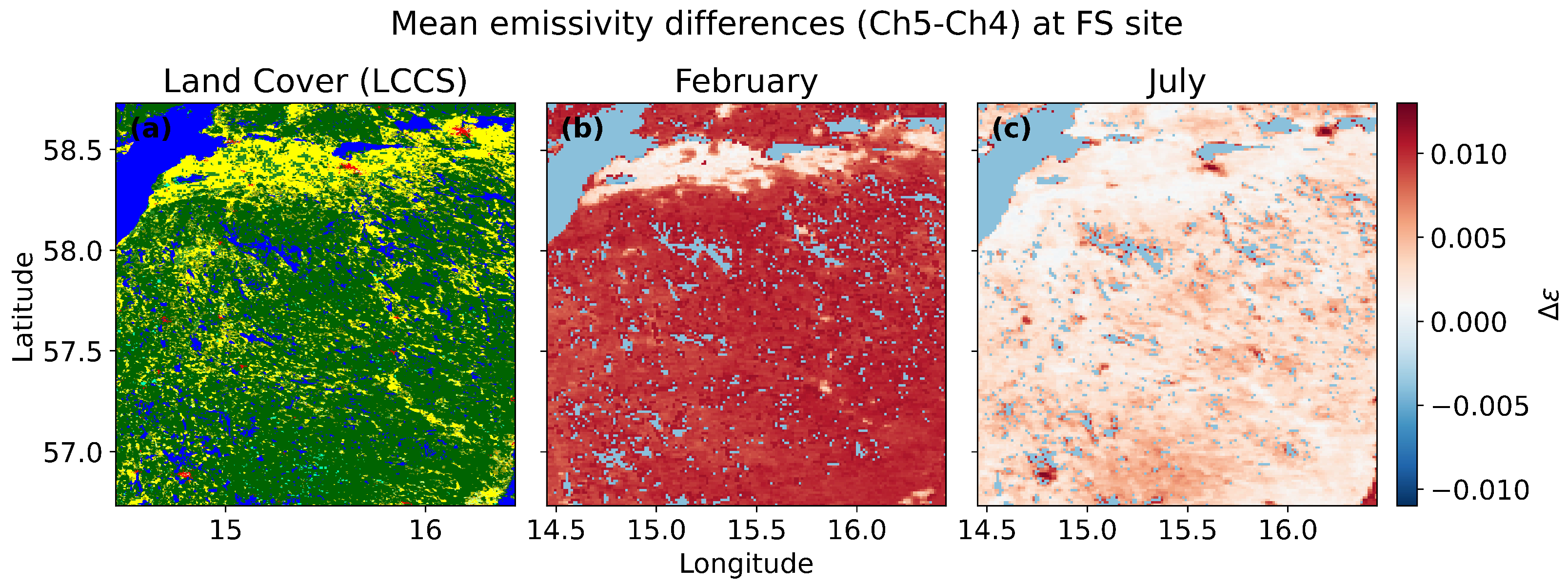
LSE difference maps (Ch5–Ch4) were generated for the two forested areas, one in the north and one in the south of Fennoscandia (Figure 7 and Figure 8). These maps were generated from the monthly mean emissivity values over the 40-year period (1981–2022). Each mapped area covers a 1° × 1° region surrounding the FN and FS sites, respectively.
In the northern area of interest (AOI) during February, the surface exhibits scattered patches of snow alongside snow-free areas with low NDVI values, indicative of vegetation post-snow melt. These patterns are reflected in the slightly negative LSE differences corresponding to snow pixels, as the emissivity of snow is higher in channel 4 than in channel 5. Positive differences can be attributed to mixed areas. Areas adjacent to water bodies display high positive differences in winter, likely representing water pixels misclassified as bare soil (NDVI < 0.2) or wet areas with low NDVI values during winter. As noted by Palmtag et al. [16], land-cover datasets often misclassify water bodies in northern high latitudes. In July, the area predominantly shows positive differences, except for water bodies, which exhibit a small negative difference.
In the southern AOI, strong positive differences are observed in February, attributed to the emissivity difference between channels 4 and 5 for bare or mixed areas with a high proportion of bare soil. Lighter regions correspond to croplands, which typically have a higher SCFV in February compared to surrounding areas. In July, mean differences are minimal, indicating that most areas are densely vegetated, with NDVI values exceeding 0.475, resulting in a similar emissivity for both channels. Urban areas, characterised by low NDVI values, exhibit high positive differences in summer due to the higher emissivity of bare soil in channel 5 compared to channel 4.

3.2. Comparison to MODIS

The AVHRR LAC LSE dataset is compared to the MODIS MOD11A2 LSE dataset, recorded from the Terra satellite series. The MODIS emissivity dataset is based on land-cover classification and dynamic and seasonal factors such as vegetation senescence and snow cover [53]. The MODIS product was chosen for the intercomparison due to its global coverage, long data coverage (from 2000 to the present), and similarities in terms of spatial and temporal resolution and spectral bandwidths of the TIR channels.
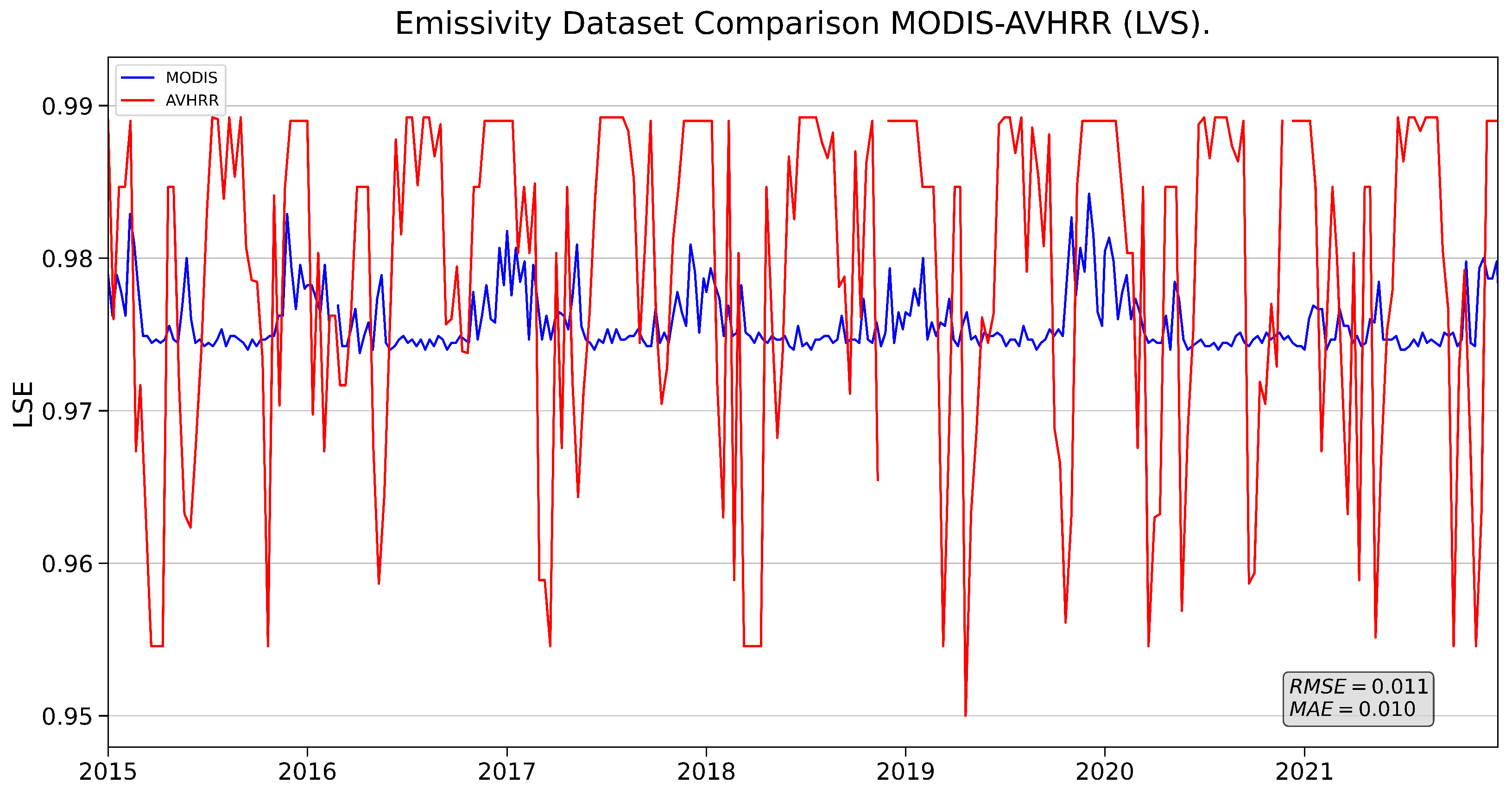
In situ data from a ground station are the most direct type of validation for comparison and are widely used in remote sensing for ground truthing [66]. However, there are no long-term measured emissivity field data available for Sweden, Norway, or Finland. Furthermore, in situ data from ground stations would not allow validation at a country scale. The MOD11A2 LSE dataset is available for two bands; band 31, at a wavelength of 10.78–11.28 µm, was chosen for comparison with AVHRR band 4, at a wavelength of 10.30–11.30 µm. Figure 9 compares the AVHRR LAC LSE dataset, derived from NDVITHM, with the MOD11A2 LSE product for the low-vegetation southern (LVS) study site. An area corresponding to a 3 × 3 pixel was selected in both datasets and averaged for the comparison.
The MODIS and AVHRR LSE datasets are substantially different due to the differing spectral responses of the sensors, varying swath widths, and orbiting geometries, as well as the different methods used to assign emissivity values to pixels with variable land cover and vegetation activity [11]. The spectral response functions of the AVHRR and MODIS sensors for the red and near-infrared channels used to calculate the NDVI values have been presented and discussed, for example, by Fan et al. [67] and Kim et al. [68], showing the significantly narrower spectral widths of the MODIS NIR and VIS channels compared to those of the AVHRR. Furthermore, differing atmospheric correction procedures and the spatial and temporal resolution of the datasets also have an impact on the emissivity dataset.
The AVHRR LAC LSE dataset exhibits stronger seasonality than the MOD11A2 LSE product. This can be explained by the fact that the AVHRR LAC LSE product relies directly on NDVI values and is not scaled by land-cover classification. During the cold season, LSE values—primarily influenced by snow—are higher in the AVHRR product. This is because the snow emissivity in the AVHRR product is based on the work of Hulley et al. [23], while the MODIS product uses laboratory spectra for the snow emissivity, which tends to result in slightly lower values [53]. Differences in the respective snow and cloud masking techniques also affect the final emissivity products. To quantify these differences, the Root Mean Square Error (RMSE) and the Mean Absolute Error (MAE) were calculated. Since the two products have different compositing periods and starting times, only the emissivity values within a 3-day tolerance window were selected for comparison. Even with this approach, a mismatch in temporal overlap persisted due to the differing composite lengths—8 days for the MODIS dataset and 10 days for the AVHRR dataset. The RMSE was found to be 0.011, and the MAE was 0.010. Despite these differences, both products effectively capture snow onset and melt patterns.

4. Discussion

4.1. Emissivity Retrieval

No single LSE retrieval method performs best; all approaches have advantages and disadvantages. The significant advantage of the NDVITHM is its applicability using only AVHRR channels 1 and 2 data, which have been available since 1981. The data processing steps outlined in Section 2.2 enabled the creation of a 40-year emissivity dataset that is both spatially and temporally comprehensive. This method produced reliable results for vegetated areas during the summer, effectively capturing vegetation dynamics. By incorporating water masks and snow-cover information, the NDVITHM can be applied to regions containing water bodies and extended to cover the entire year, including snow-covered periods. Additionally, this method does not require accurate atmospheric correction when estimating vegetation cover from the NDVI [26].
The drawbacks of the NDVITHM are its dependence on the NDVI (an index that is itself subject to uncertainties), the need for auxiliary data to map snow and water accurately, and areas without NDVI-relevant vegetation (such as lichens or senescent vegetation). The dependence of the method on fixed thresholds and values can also introduce errors. For instance, in mixed pixels containing both vegetation and bare soil, daytime emission from soil surfaces—which is subject to strong solar absorption—can dominate, with shadowing effects further complicating the emissivity estimation [9]. Furthermore, vegetation indices are unable to distinguish between bare soils and dormant vegetation, which can lead to an underestimation of the vegetation fraction [23]. Despite these disadvantages, the AVHRR LAC LSE dataset presented here is a good basis and provides 40 years of data, which cannot be retrieved using any other sensor. The high temporal resolution enables the monitoring of both seasonal and abrupt changes in vegetation canopy.
NDVI compositing is a commonly used method when producing time series to minimise errors and disturbances such as cloud contamination, effects of aerosols and water vapour in the atmosphere, directional reflectance and off-nadir viewing effects, and sun-angle and shadow effects [69]. Based on the detailed study by Asam et al. [70], the Median NDVI Compositing Method (MED) was chosen over the Maximum Value Compositing Method (MVC), which is often applied to AVHRR data. Asam et al. [70] showed that the MVC approach leads to a general overestimation of the NDVI, as often pixels affected by signal saturation or pixels from off-nadir angles are selected, and artefacts such as scan lines can occur. Using the MED leads to a smoother and more consistent dataset without geometric artefacts, and while it results in overall lower NDVI values, the data distribution is more consistent and without saturation.

4.2. Time Series

The time series, as plotted in Figure 5, for the LVS study site presents strong periodicity. These variabilities are mainly due to seasonal vegetation changes, with lower NDVI values in autumn and spring because of the inactive vegetation. The high emissivity values are due to the healthy, dense vegetation canopy in summer and the snow cover in winter.
Despite the good temporal resolution of the AVHRR, not all years are covered equally well due to compromised data caused by missed scan lines or unusual satellite manoeuvring and errors occurring during the processing steps, such as automated geolocation [71], leading to significant gaps in the dataset, mainly prominent before the year 2000 (Figure 4). In the earlier years, only one or two satellites carrying AVHRR sensors were operational simultaneously, resulting in no redundancy in case of an outage. To avoid assigning incorrect emissivity values, these gaps are not interpolated. Starting around the year 2000, with the launch of NOAA-16 and NOAA-17 in relatively quick succession (2000 and 2002), the data coverage greatly increased, with four or five AVHRR sensors being in orbit at the same time, providing overlapping datasets. Data gaps are also due to the inability to record the NDVI values during the polar night at high latitudes or extensive cloud cover over a longer period.

4.3. Impact of Land Cover and Latitude

As seen in Table 3, the emissivity is generally higher for the same land cover at the southern study sites than at the northern sites. This follows the latitudinal gradient of the NDVI, as described by Jia et al. [72], with generally lower NDVI values in the northern latitudes and a gradual increase in the index towards the southern regions. The gradient is partly explained by the growing season’s length, which generally starts earlier with decreasing latitude due to higher temperatures and higher moisture availability in the southern regions. Biomass and the leaf area index (LAI), which have been identified as significant factors influencing the NDVI, are expected to follow a similar latitudinal pattern. These factors positively impact the vegetation in the more southern regions, leading to an increased NDVI and, thus, higher emissivity values.
In summer, the emissivity is higher for the forested study sites than for the low vegetation sites, as the dense forests generally have a slightly higher NDVI than the smaller plant cover consisting of shrubs or heaths. However, in winter, the emissivity is generally higher at the low-vegetation sites, as a more uniform snowpack can form on the low vegetation. Due to the polar night, NDVI retrieval is not possible during the dark winter months at the high-latitude study sites, leading to data gaps in November, December, and January.

4.4. Comparison to MODIS

The direct comparison between the MOD11A2 and AVHRR LAC LSE datasets in Figure 9 shows clear differences in emissivity estimations based on the two different methods. The MODIS MOD11A2 emissivity product is based on lookup tables, including land cover, vegetation dynamics, and snow cover, which can result in a smoothing of extreme values during the winter or summer seasons. Conversely, the AVHRR LAC LSE dataset is based on 10-day composites calculated from daily NDVI data. The low emissivity values in the AVHRR dataset are mainly due to seasonal vegetation changes, with lower NDVI values in autumn and spring. The high emissivity values are due to the healthy, dense vegetation canopy in summer and the snow cover in winter.
The interplay of various factors, like the onset or melt of the snowpack and seasonal vegetation patterns, leads to a varied emissivity curve throughout the seasons and variation from year to year. In addition to the regular yearly vegetation cycle, an NDVI-based method is also able to record vegetation changes, such as loss of foliage due to droughts, pests, or fires, or sudden canopy changes due to deforestation or severe storms. Heterogeneous pixels, which are difficult to assign to one specific land-cover class, might also be easier to record with the NDVI method as the vegetation activity is measured.
The values set for the different land-cover types in the MODIS dataset are higher than the values proposed by Sobrino et al. [28] and those chosen for the calculation of the AVHRR LAC LSE dataset. This leads to fundamental differences between the datasets, as apparent in Figure 9, which can exceed 0.02, resulting in a temperature difference of approximately 2 K, as shown in Schädlich et al. [13].

4.5. Uncertainty Sources

Sub-pixel variation, i.e., when the land cover is fragmented on a smaller scale than the available spatial resolution of the sensor, which is easily the case when using AVHRR data with a medium spatial resolution of 1.1 × 1.1 km at nadir, might introduce some uncertainties. The likely sub-pixel variability, with different vegetation types, bare soil areas, and water bodies alternating, can lead to uncertainties and anomalies in the NDVI calculation. The same problem arises with regard to the snow mask. Snow pixels are classified as such if the parameter snow-cover fraction viewable in the dataset is 70% or higher. Therefore, a pixel could theoretically be covered by 70% snow and 30% vegetation or soil but would obtain the emissivity value for snow assigned, resulting in an overestimation of the emissivity in that pixel. This is the typical trade-off in remote sensing between high spatial and high temporal resolution. The medium spatial resolution of the AVHRR is balanced by the high temporal frequency of the daily data.

4.6. Limitations

The approach presented in this study, with its long time series and high temporal resolution, is unique but comes with several limitations that should be considered for any application. The spatial resolution of the AVHRR sensor inherently results in mixed-pixel data, where the emissivity values are primarily influenced by the dominant land cover within each pixel. As a result, 20–40% of the pixel’s surface area may be under-represented in the final emissivity value. However, this issue is common to all medium-resolution sensors. Additionally, despite good geocoding accuracy that meets the requirements of the GCOS, a pixel shift of 300 m can lead to incorrect allocation of the snow mask or land-cover information, affecting the emissivity retrieval. Moreover, the emissivity retrieval used in this study depends on visible channels, which are unavailable at night, limiting data collection during the polar night. These visible channels are also restricted to clear-sky conditions, further reducing the number of valid satellite images. Persistent cloud cover can prevent accurate monitoring of vegetation dynamics, leading to the under-representation of actual emissivity changes, particularly during periods of high variability.

5. Conclusions

In this study, a 40-year land surface emissivity dataset for the period 1981–2022 was created using the NDVITHM adapted from Sobrino et al. [28]. While the emissivity dataset encompasses all of Europe, the analysis was restricted to Norway, Sweden, and Finland. The dataset was derived from the AVHRR LAC L1C data with a spatial resolution of 1.1 km at nadir and a temporal resolution of 10 days. The dataset comprises a water mask and a snow mask, providing emissivity data for vegetated as well as water- and snow-covered areas.
The comparison with the MODIS MOD11A2 LSE dataset shows that the two datasets lie in a similar range but still exhibit significant differences. When considering the differences in wavelengths, temporal resolution, and the chosen method and fixed values used to calculate the emissivity, the disparities can be well explained, and the NDVITHM also produces satisfactory results. In comparison to other emissivity products, the main advantage of the AVHRR LAC LSE dataset lies in its temporal coverage (1981–2022). In addition, the daily resolution of the AVHRR LAC data, on which the composites are based, allows for the recording of rapid changes in vegetation, such as forest fires, deforestation, large-scale forestry operations, or the onset and end of the growing season and snowfall or snow melt.
The NDVITHM method was tailored for Fennoscandia, but the area of application could be expanded further by adjusting the NDVI thresholds and fixed emissivity values specifically to the regional and biogeographical characteristics.

Author Contributions

Conceptualisation, S.D., S.W. and M.B.; methodology, S.D., S.W. and M.B.; software, S.D. and M.B.; investigation, M.B.; data curation, S.D.; writing—original draft preparation, M.B. and S.D.; writing—review and editing, S.D., S.W. and M.B.; visualisation, M.B. and S.D.; supervision, S.W. and S.D.; project administration, S.W. and S.D. All authors have read and agreed to the published version of the manuscript.

Funding

This research received no external funding.

Data Availability Statement

The AVHRR NDVI dataset used in this study is available from the repository of the University of Bern, https://boris-portal.unibe.ch/handle/20.500.12422/449, accessed on 20 May 2024.

Acknowledgments

We thank Christoph Neuhaus for his help with data processing, and we are very grateful for Helga Weber’s advice on AVHRR data analysis. We also thank Helga Weber for providing the 40-year snow-cover data derived from the AVHRR LAC data.

Conflicts of Interest

The authors declare no conflicts of interest.

References

  1. Valor, E. Mapping land surface emissivity from NDVI: Application to European, African, and South American areas. Remote Sens. Environ. 1996, 57, 167–184. [Google Scholar] [CrossRef]
  2. Hulley, G.C.; Hook, S.J.; Abbott, E.; Malakar, N.; Islam, T.; Abrams, M. The ASTER Global Emissivity Dataset (ASTER GED): Mapping Earth’s emissivity at 100 meter spatial scale. Geophys. Res. Lett. 2015, 42, 7966–7976. [Google Scholar] [CrossRef]
  3. Li, Z.; Wu, H.; Duan, S.; Zhao, W.; Ren, H.; Liu, X.; Leng, P.; Tang, R.; Ye, X.; Zhu, J.; et al. Satellite Remote Sensing of Global Land Surface Temperature: Definition, Methods, Products, and Applications. Rev. Geophys. 2023, 61, e2022RG000777. [Google Scholar] [CrossRef]
  4. Global Climate Observing System (GCOS). The Global Observing System for Climate: Implementation Needs; Technical Report GCOS-200; World Meteorological Organization: Geneva, Switzerland, 2016. [Google Scholar]
  5. Chao, Q.; Han Dolman, A.J.; Herold, M.; Krug, T.; Speich, S.; Suda, K.; Thorne, P.; Yu, W.; Zemp, M. GCOS 2022 Implementation Plan; Technical Report; World Meteorological Organization: Geneva, Switzerland, 2022. [Google Scholar] [CrossRef]
  6. Li, Z.L.; Tang, B.H.; Wu, H.; Ren, H.; Yan, G.; Wan, Z.; Trigo, I.F.; Sobrino, J.A. Satellite-derived land surface temperature: Current status and perspectives. Remote Sens. Environ. 2013, 131, 14–37. [Google Scholar] [CrossRef]
  7. Li, Z.L.; Wu, H.; Wang, N.; Qiu, S.; Sobrino, J.A.; Wan, Z.; Tang, B.H.; Yan, G. Land surface emissivity retrieval from satellite data. Int. J. Remote Sens. 2013, 34, 3084–3127. [Google Scholar] [CrossRef]
  8. Wan, Z.; Dozier, J. A generalized split-window algorithm for retrieving land-surface temperature from space. IEEE Trans. Geosci. Remote Sens. 1996, 34, 892–905. [Google Scholar] [CrossRef]
  9. Ghent, D.J.; Corlett, G.K.; Göttsche, F.M.; Remedios, J.J. Global Land Surface Temperature From the Along-Track Scanning Radiometers. J. Geophys. Res. Atmos. 2017, 122, 12167–12193. [Google Scholar] [CrossRef]
  10. Waring, A.M.; Ghent, D.; Perry, M.; Anand, J.S.; Veal, K.L.; Remedios, J. Regional climate trend analyses for Aqua MODIS land surface temperatures. Int. J. Remote Sens. 2023, 44, 4989–5032. [Google Scholar] [CrossRef]
  11. Jiménez-Muñoz, J.C.; Sobrino, J.A.; Gillespie, A.; Sabol, D.; Gustafson, W.T. Improved land surface emissivities over agricultural areas using ASTER NDVI. Remote Sens. Environ. 2006, 103, 474–487. [Google Scholar] [CrossRef]
  12. Neinavaz, E.; Schlerf, M.; Darvishzadeh, R.; Gerhards, M.; Skidmore, A.K. Thermal infrared remote sensing of vegetation: Current status and perspectives. Int. J. Appl. Earth Obs. Geoinf 2021, 102, 102415. [Google Scholar] [CrossRef]
  13. Schädlich, S. Influence of Land Surface Parameters and Atmosphere on METEOSAT Brightness Temperatures and Generation of Land Surface Temperature Maps by Temporally and Spatially Interpolating Atmospheric Correction. Remote Sens. Environ. 2001, 75, 39–46. [Google Scholar] [CrossRef]
  14. Sobrino, J.; Coll, C.; Caselles, V. Atmospheric correction for land surface temperature using NOAA-11 AVHRR channels 4 and 5. Remote Sens. Environ. 1991, 38, 19–34. [Google Scholar] [CrossRef]
  15. Becker, F. The impact of spectral emissivity on the measurement of land surface temperature from a satellite. Int. J. Remote Sens. 1987, 8, 1509–1522. [Google Scholar] [CrossRef]
  16. Palmtag, J.; Obu, J.; Kuhry, P.; Richter, A.; Siewert, M.B.; Weiss, N.; Westermann, S.; Hugelius, G. A high spatial resolution soil carbon and nitrogen dataset for the northern permafrost region based on circumpolar land cover upscaling. Earth Syst. Sci. Data 2022, 14, 4095–4110. [Google Scholar] [CrossRef]
  17. Rantanen, M.; Kämäräinen, M.; Niittynen, P.; Phoenix, G.K.; Lenoir, J.; Maclean, I.; Luoto, M.; Aalto, J. Bioclimatic atlas of the terrestrial Arctic. Sci. Data 2023, 10, 40. [Google Scholar] [CrossRef]
  18. Pearson, R.G.; Phillips, S.J.; Loranty, M.M.; Beck, P.S.; Damoulas, T.; Knight, S.J.; Goetz, S.J. Shifts in Arctic vegetation and associated feedbacks under climate change. Nat. Clim. Change 2013, 3, 673–677. [Google Scholar] [CrossRef]
  19. Sturm, M.; Schimel, J.; Michaelson, G.; Welker, J.M.; Oberbauer, S.F.; Liston, G.E.; Fahnestock, J.; Romanovsky, V.E. Winter Biological Processes Could Help Convert Arctic Tundra to Shrubland. BioScience 2005, 55, 17–26. [Google Scholar] [CrossRef]
  20. Wielgolaski, F.E. (Ed.) Fennoscandian Tundra Ecosystems: Part 1 Plants and Microorganisms, 1st ed.; Ecological Studies; Springer: Berlin/Heidelberg, Germany, 1975; Volume 16, p. 368. [Google Scholar] [CrossRef]
  21. Lagergren, F.; Björk, R.G.; Andersson, C.; Belušić, D.; Björkman, M.P.; Kjellström, E.; Lind, P.; Lindstedt, D.; Olenius, T.; Pleijel, H.; et al. Kilometre-scale simulations over Fennoscandia reveal a large loss of tundra due to climate warming. Biogeosciences 2024, 21, 1093–1116. [Google Scholar] [CrossRef]
  22. Liu, C.; Huang, H.; Liu, C.; Wang, X.; Wang, S. Comparative evaluation of vegetation greenness trends over circumpolar Arctic tundra using multi-sensors satellite datasets. Int. J. Digi. Earth 2024, 17, 2328823. [Google Scholar] [CrossRef]
  23. Hulley, G.; Veraverbeke, S.; Hook, S. Thermal-based techniques for land cover change detection using a new dynamic MODIS multispectral emissivity product (MOD21). Remote Sens. Environ. 2014, 140, 755–765. [Google Scholar] [CrossRef]
  24. Hüsler, F.; Fontana, F.; Neuhaus, C.; Riffler, M.; Musial, J.; Wunderle, S. AVHRR Archive and Processing Facility at the University of Bern: A comprehensive 1-km satellite data set for climate change studies. EARSeL eProceedings 2011, 10, 83–101. [Google Scholar]
  25. Trigo, I.F.; Peres, L.F.; DaCamara, C.C.; Freitas, S.C. Thermal Land Surface Emissivity Retrieved From SEVIRI/Meteosat. IEEE Trans. Geosci. Remote Sens. 2008, 46, 307–315. [Google Scholar] [CrossRef]
  26. Sobrino, J.A.; Jimenez-Munoz, J.C.; Soria, G.; Romaguera, M.; Guanter, L.; Moreno, J.; Plaza, A.; Martinez, P. Land Surface Emissivity Retrieval From Different VNIR and TIR Sensors. IEEE Trans. Geosci. Remote Sens. 2008, 46, 316–327. [Google Scholar] [CrossRef]
  27. Sobrino, J.A.; Raissouni, N. Toward remote sensing methods for land cover dynamic monitoring: Application to Morocco. Int. J. Remote Sens. 2000, 21, 353–366. [Google Scholar] [CrossRef]
  28. Sobrino, J. A Comparative Study of Land Surface Emissivity Retrieval from NOAA Data. Remote Sens. Environ. 2001, 75, 256–266. [Google Scholar] [CrossRef]
  29. Xue, S.Y.; Xu, H.Y.; Mu, C.C.; Wu, T.H.; Li, W.P.; Zhang, W.X.; Streletskaya, I.; Grebenets, V.; Sokratov, S.; Kizyakov, A.; et al. Changes in different land cover areas and NDVI values in northern latitudes from 1982 to 2015. Adv. Clim. Change Res. 2021, 12, 456–465. [Google Scholar] [CrossRef]
  30. Wan, Z.; Hook, S.; Hulley, G. MODIS/Terra Land Surface Temperature/Emissivity 8-Day L3 Global 1 km SIN Grid V061; Technical Report; USGS: Reston, VA, USA, 2021. [CrossRef]
  31. World Meteorological Organization. Implementation Plan for the Global Observing System for Climate in Support of the UNFCCC; Technical Report GOOS-184, GTOS-76, WMO-TD/No. 1523; World Meteorological Organization (WMO): Geneva, Switzerland, 2010. [Google Scholar]
  32. Becker, F.; Li, Z. Surface temperature and emissivity at various scales: Definition, measurement and related problems. Remote Sens. Rev. 1995, 12, 225–253. [Google Scholar] [CrossRef]
  33. Cheng, J.; Liang, S.; Meng, X.; Quan, Z.; Zhou, S. Chapter 7—Land surface temperature and thermal infrared emissivity. In Advanced Remote Sensing, 2nd ed.; Liang, S., Wang, J., Eds.; Academic Press: Cambridge, MA, USA, 2020; pp. 251–295. [Google Scholar] [CrossRef]
  34. McCluney, W.R. Introduction to Radiometry and Photometry, 2nd ed.; Artech House: Norwood, MA, USA, 2014. [Google Scholar]
  35. Quattrochi, D.A.; Luvall, J.C. (Eds.) Thermal Remote Sensing in Land Surface Processes, 1st ed.; CRC Press: Boca Raton, FL, USA, 2004. [Google Scholar] [CrossRef]
  36. Stathopoulou, M.; Cartalis, C.; Petrakis, M. Integrating Corine Land Cover data and Landsat TM for surface emissivity definition: Application to the urban area of Athens, Greece. Int. J. Remote Sens. 2007, 28, 3291–3304. [Google Scholar] [CrossRef]
  37. Jin, M.; Liang, S. An Improved Land Surface Emissivity Parameter for Land Surface Models Using Global Remote Sensing Observations. J. Clim. 2006, 19, 2867–2881. [Google Scholar] [CrossRef]
  38. Van De Griend, A.A.; Owe, M. On the relationship between thermal emissivity and the normalized difference vegetation index for natural surfaces. Int. J. Remote Sens. 1993, 14, 1119–1131. [Google Scholar] [CrossRef]
  39. Pinheiro, A.; Mahoney, R.; Privette, J.; Tucker, C. Development of a daily long term record of NOAA-14 AVHRR land surface temperature over Africa. Remote Sens. Environ. 2006, 103, 153–164. [Google Scholar] [CrossRef]
  40. Dozier, J.; Warren, S.G. Effect of viewing angle on the infrared brightness temperature of snow. Water Resour. Res. 1982, 18, 1424–1434. [Google Scholar] [CrossRef]
  41. Meerdink, S.K.; Hook, S.J.; Roberts, D.A.; Abbott, E.A. The ECOSTRESS spectral library version 1.0. Remote Sens. Environ. 2019, 230, 111196. [Google Scholar] [CrossRef]
  42. Baldridge, A.; Hook, S.; Grove, C.; Rivera, G. The ASTER spectral library version 2.0. Remote Sens. Environ. 2009, 113, 711–715. [Google Scholar] [CrossRef]
  43. European Space Agency (ESA). Land Cover CCI Product User Guide Version 2. Technical Report, European Space Agency. 2017. Available online: http://maps.elie.ucl.ac.be/CCI/viewer/download/ESACCI-LC-Ph2-PUGv2_2.0.pdf (accessed on 20 May 2024).
  44. Weber, H.; Naegeli, K.; Wunderle, S. Impact of Forest Canopy Parameterization on Space-Borne Snow on Ground Detection. In Proceedings of the 2021 IEEE International Geoscience and Remote Sensing Symposium IGARSS, Brussels, Belgium, 11–16 July 2021; pp. 864–867. [Google Scholar] [CrossRef]
  45. Emery, W.; Camps, A. Chapter 9—Ocean Applications. In Introduction to Satellite Remote Sensing; Elsevier: Amsterdam, The Netherlands, 2017; pp. 637–699. [Google Scholar] [CrossRef]
  46. Wunderle, S.; Neuhaus, C.; Brooks, A.; Hüsler, F.; Lonie, N.; Albani, M.; Folco, S.; Leone, R. Preservation and harmonization of historical AVHRR LAC data to serve the needs of users in climate research. In Proceedings of the 2017 Conference on Big Data from Space (BIDS’ 2017), Toulouse, France, 28–30 November 2017. [Google Scholar] [CrossRef]
  47. Khlopenkov, K.; Trishchenko, A.; Luo, Y. Achieving Subpixel Georeferencing Accuracy in the Canadian AVHRR Processing System. IEEE Trans. Geosci. Remote Sens. 2010, 48, 2150–2161. [Google Scholar] [CrossRef]
  48. Aksakal, S.; Neuhaus, C.; Baltsavias, E.; Schindler, K. Geometric Quality Analysis of AVHRR Orthoimages. Remote Sens. 2015, 7, 3293–3319. [Google Scholar] [CrossRef]
  49. EUMETSAT. AVHRR Level 1b Product Guide; Technical Report; EUMETSAT: Darmstadt, Germany, 2011. [Google Scholar]
  50. Heidinger, A.K.; Straka, W.C.; Molling, C.C.; Sullivan, J.T.; Wu, X. Deriving an inter-sensor consistent calibration for the AVHRR solar reflectance data record. Int. J. Remote Sens. 2010, 31, 6493–6517. [Google Scholar] [CrossRef]
  51. Kidwell, K.B. NOAA Polar Orbiter Data (POD) User’s Guide (TIROS-N, NOAA-6, -7, -8, -9, -10, -11, -12, -13 and -14); Technical Report; NOAA: Washington, DC, USA, 1998.
  52. Walton, C.C.; Sullivan, J.T.; Rao, C.R.N.; Weinreb, M.P. Corrections for detector nonlinearities and calibration inconsistencies of the infrared channels of the advanced very high resolution radiometer. J. Geophys Res. Ocean. 1998, 103, 3323–3337. [Google Scholar] [CrossRef]
  53. Snyder, W.C.; Wan, Z.; Zhang, Y.; Feng, Y.Z. Classification-based emissivity for land surface temperature measurement from space. Int. J. Remote Sens. 1998, 19, 2753–2774. [Google Scholar] [CrossRef]
  54. SMHI. The NWC SAF/PPS. Available online: https://nwcsaf.smhi.se/ (accessed on 12 June 2024).
  55. Fontana, F.M.; Trishchenko, A.P.; Khlopenkov, K.V.; Luo, Y.; Wunderle, S. Impact of orthorectification and spatial sampling on maximum NDVI composite data in mountain regions. Remote Sens. Environ. 2009, 113, 2701–2712. [Google Scholar] [CrossRef]
  56. Trishchenko, A.P.; Cihlar, J.; Li, Z. Effects of spectral response function on surface reflectance and NDVI measured with moderate resolution satellite sensors. Remote Sens. Environ. 2002, 81, 1–18. [Google Scholar] [CrossRef]
  57. Trishchenko, A.P. Effects of spectral response function on surface reflectance and NDVI measured with moderate resolution satellite sensors: Extension to AVHRR NOAA-17, 18 and METOP-A. Remote Sens. Environ. 2009, 113, 335–341. [Google Scholar] [CrossRef]
  58. Lieberherr, G.; Wunderle, S. Lake Surface Water Temperature Derived from 35 Years of AVHRR Sensor Data for European Lakes. Remote Sens. 2018, 10, 990. [Google Scholar] [CrossRef]
  59. Dupuis, S.; Rivoire, P.; Barben, M.; Wunderle, S. 40-Year AVHRR Top-of-Atmosphere NDVI Dataset. 2024. Available online: https://boris-portal.unibe.ch/entities/product/158bc761-44d4-4b55-a33e-03474768c592 (accessed on 20 May 2024). [CrossRef]
  60. Jacob, F.; Lesaignoux, A.; Olioso, A.; Weiss, M.; Caillault, K.; Jacquemoud, S.; Nerry, F.; French, A.; Schmugge, T.; Briottet, X.; et al. Reassessment of the temperature-emissivity separation from multispectral thermal infrared data: Introducing the impact of vegetation canopy by simulating the cavity effect with the SAIL-Thermique model. Remote Sens. Environ. 2017, 198, 160–172. [Google Scholar] [CrossRef]
  61. Sobrino, J.; Caselles, V.; Becker, F. Significance of the remotely sensed thermal infrared measurements obtained over a citrus orchard. ISPRS J. Photogramm. Remote Sens. 1990, 44, 343–354. [Google Scholar] [CrossRef]
  62. Lillesand, T.; Kiefer, R.; Chipman, J. Chapter 4—Multispectral, Thermal and Hyperspectral Sensing. In Remote Sensing and Image Interpretation, 7th ed.; John Wiley: Hoboken, NJ, USA, 2015. [Google Scholar]
  63. Korchagina, I.; Goleva, O.; Savchenko, Y.; Bozhikov, T. The use of geographic information systems for forest monitoring. J. Phys. Conf. Ser. 2020, 1515, 032077. [Google Scholar] [CrossRef]
  64. Weber, H. GCOS Switzerland Project: Fractional Snow Cover Time Series (1981–2021)—A Novel Dataset from Space to Support Climate Studies in Switzerland, Final Report; Technical Report; Federal Office of Meteorology and Climatology—MeteoSwiss: Zurich, Switzerland, 2022. [Google Scholar]
  65. Obrecht, L.; Göttsche, F.M.; Senn, J.A.; Cermak, J. Mapping Changes in Fractional Vegetation Cover on the Namib Gravel Plains with Satellite-Retrieved Land Surface Emissivity Data. Remote Sens. 2024, 16, 159. [Google Scholar] [CrossRef]
  66. Nagol, J.R. Quantification of Error in AVHRR NDVI Data. Ph.D. Thesis, University of Maryland, College Park, MD, USA, 2011. [Google Scholar]
  67. Fan, X.; Liu, Y. A global study of NDVI difference among moderate-resolution satellite sensors. ISPRS J. Photogramm. Remote Sens. 2016, 121, 177–191. [Google Scholar] [CrossRef]
  68. Kim, Y.; Huete, A.; Jiang, Z.; Miura, T. Multisensor reflectance and vegetation index comparisons of Amazon tropical forest phenology with hyperspectral Hyperion data. SPIE Conf. Proc. 2007, 6679, 54–63. [Google Scholar] [CrossRef]
  69. Holben, B.N. Characteristics of maximum-value composite images from temporal AVHRR data. Int. J. Remote Sens. 1986, 7, 1417–1434. [Google Scholar] [CrossRef]
  70. Asam, S.; Eisfelder, C.; Hirner, A.; Reiners, P.; Holzwarth, S.; Bachmann, M. AVHRR NDVI Compositing Method Comparison and Generation of Multi-Decadal Time Series—A TIMELINE Thematic Processor. Remote Sens. 2023, 15, 1631. [Google Scholar] [CrossRef]
  71. Tomlinson, C.J.; Chapman, L.; Thornes, J.E.; Baker, C. Remote sensing land surface temperature for meteorology and climatology: A review. Meteorol. Appl. 2011, 18, 296–306. [Google Scholar] [CrossRef]
  72. Jia, G.J.; Epstein, H.E.; Walker, D.A. Spatial characteristics of AVHRR-NDVI along latitudinal transects in northern Alaska. J. Veg. Sci. 2002, 13, 315–326. [Google Scholar] [CrossRef]
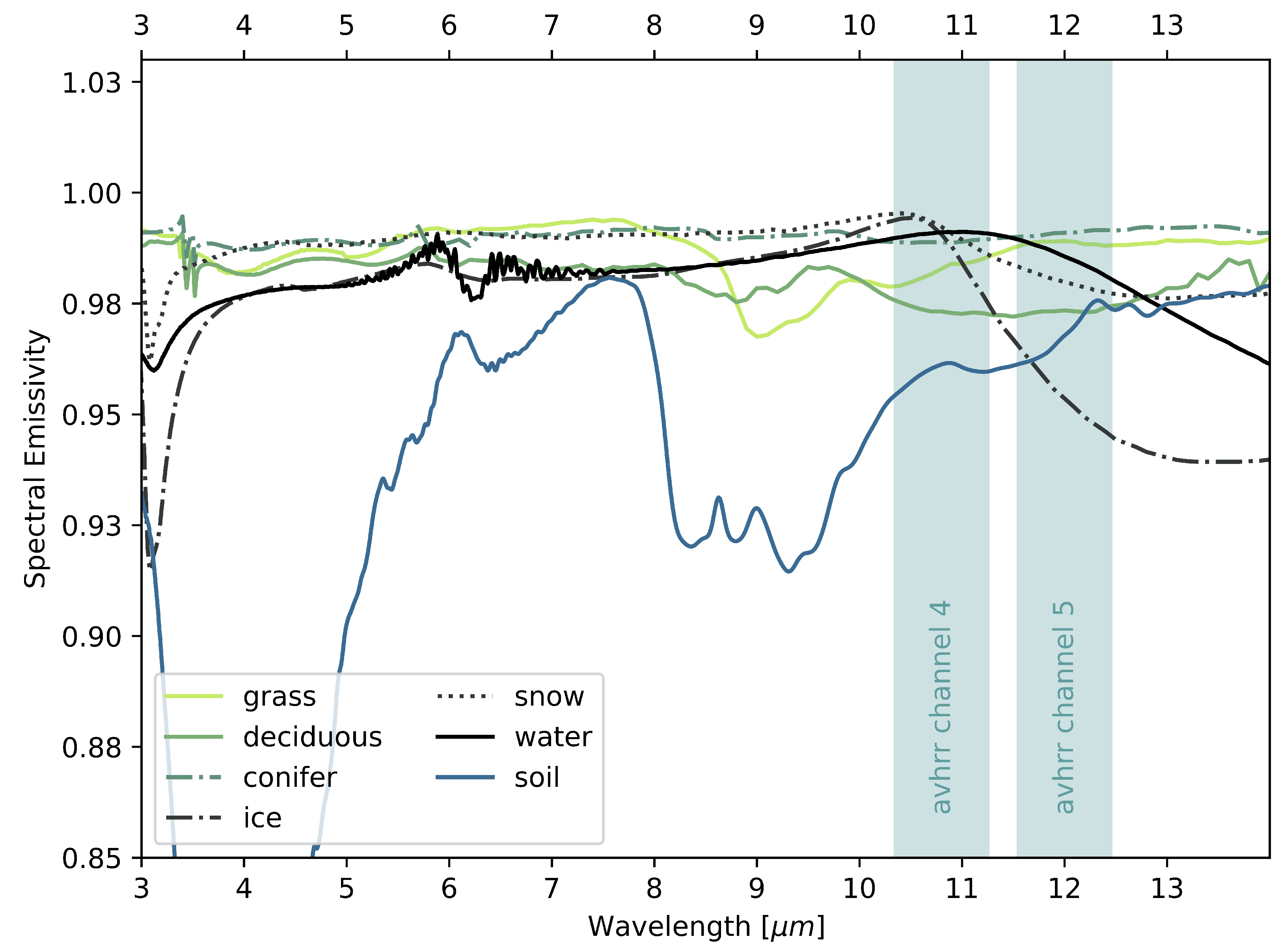
Figure 1. Spectral emissivities of different land-cover classes, as recorded in the ECOSTRESS spectral library [41,42].
Remotesensing 16 03686 g001
Figure 2. The study area across Norway, Sweden, and Finland, showing the six chosen study sites (15 × 15 km each). The abbreviations indicating the study sites stand for Low Vegetation (LV) or Forest (F) and South (S), Mid-Latitude (ML), or North (N). The base map is the ESA CCI Land-Cover Dataset [43].
Remotesensing 16 03686 g002
Figure 3. Schematic workflow showing the AVHRR data preparation, emissivity dataset calculation process, and incorporated auxiliary data.
Remotesensing 16 03686 g003
Figure 4. Overview of the availability of AVHRR data since 1981 in the local archive. The data used for this study are indicated in blue-grey, while the data excluded from the analysis due to quality or processing issues are indicated in orange.
Remotesensing 16 03686 g004
Figure 5. The 40-year time series of monthly mean land surface emissivities for the 15 × 15 km low-vegetation southern (LVS) study site.
Remotesensing 16 03686 g005
Figure 6. Mean annual cycle of LSE for channel 4, including the confidence interval (1 σ ), for the 40-year period for the 15 × 15 km low-vegetation southern (LVS) study site.
Remotesensing 16 03686 g006
Figure 7. (a) Land cover (ESA CCI; see Figure 2 for details) and emissivity differences (Ch5–Ch4) derived from the monthly mean emissivity values over the 40-year period (1981–2022) for an area of 1° × 1° around the FN site in February (b) and July (c).
Remotesensing 16 03686 g007
Figure 8. (a) Land cover (ESA CCI; see Figure 2 for details) and emissivity differences (Ch5–Ch4) derived from the monthly mean emissivity values over the 40-year period (1981–2022) for an area of 1° × 1° around the FS site in February (b) and July (c).
Remotesensing 16 03686 g008
Figure 9. Comparison of the AVHRR LAC LSE dataset and the MODIS MOD11A2 LSE dataset for the low-vegetation southern (LVS) study site (2015–2022).
Remotesensing 16 03686 g009
Table 1. Study sites with latitudes and longitudes, as well as the prevalent land cover.
Study SiteLatitudeLongitudeLand Cover
Low Vegetation South (LVS)58.677.28Mosaic herbaceous cover (>50%)/tree and shrub (<50%)
Forest South (FS)57.7315.45Tree cover, needle-leaved, evergreen
Low Vegetation Mid-Latitude (LVML)65.0714.46Sparse vegetation
Forest Mid-Latitude (FML)64.4118.49Tree cover, needle-leaved, evergreen
Low Vegetation North (LVN)67.9419.46Sparse vegetation
Forest North (FN)66.8926.02Tree cover, needle-leaved, evergreen
Table 2. Monthly mean, minimum, and maximum NDVI values over the 40-year period for channels 4 and 5 at the two southern study sites (forest (FS) and low vegetation (LVS)).
MonthMean FSMin FSMax FSMean LVSMin LVSMax LVS
January0.143−0.1950.3190.001−0.0900.059
February0.182−0.0980.418−0.005−0.1180.134
March0.2340.0190.425−0.018−0.0960.136
April0.2960.0490.465−0.035−0.0980.120
May0.3590.0660.5250.088−0.1140.380
June0.4100.1370.5660.3400.0280.521
July0.4020.1900.5960.4410.2660.635
August0.3840.1760.5660.4210.2040.590
September0.3440.0060.5580.334−0.0110.555
October0.265−0.0180.4650.200−0.0500.430
November0.117−0.1020.3660.081−0.1340.318
December0.119−0.0570.262−0.05−0.1100.070
Table 3. Monthly mean and difference in emissivity values over the 40-year period (1981–2022) for channels 4 and 5 at the two southern and northern study sites (forest (FS) and low vegetation (LVS)).
MonthCh4 ϵ FSCh5 ϵ FS Δ ϵ FSCh4 ϵ LVSCh5 ϵ LVS Δ ϵ LVSCh4 ϵ FNCh5 ϵ FN Δ ϵ FNCh4 ϵ LVNCh5 ϵ LVN Δ ϵ LVN
January0.9650.9710.0060.9820.978−0.0040.9880.982−0.0060.9890.982−0.007
February0.9610.9710.010.9660.970−0.0040.9700.9710.0010.9790.976−0.007
March0.9640.9730.0090.9610.966−0.0050.9550.9630.0070.9610.9660.005
April0.9700.9790.0090.9650.969−0.0040.9560.9640.0080.9530.9620.009
May0.9760.9830.0070.9640.9700.0060.9600.9700.010.9610.9660.005
June0.9810.9850.0040.9740.9810.0070.9710.9800.0090.9620.9720.010
July0.9810.9850.0040.9840.9870.0050.9750.9820.0070.9750.9820.007
August0.9780.9840.0060.9830.9860.0030.9740.9810.0070.9750.9820.007
September0.9760.9820.0060.9760.9820.0060.9670.9770.010.9670.9760.009
October0.9680.9770.0090.9670.9750.0080.9640.9710.0060.9730.9740.001
November0.9650.9730.0080.9730.9740.0010.9890.982−0.0070.9890.982−0.007
December0.9860.980−0.0060.9890.982−0.007nannannannannannan
Disclaimer/Publisher’s Note: The statements, opinions and data contained in all publications are solely those of the individual author(s) and contributor(s) and not of MDPI and/or the editor(s). MDPI and/or the editor(s) disclaim responsibility for any injury to people or property resulting from any ideas, methods, instructions or products referred to in the content.