Abstract
The integration of satellite data with deep learning has revolutionized various tasks in remote sensing, including classification, object detection, and semantic segmentation. Cloud segmentation in high-resolution satellite imagery is a critical application within this domain, yet progress in developing advanced algorithms for this task has been hindered by the scarcity of specialized datasets and annotation tools. This study addresses this challenge by introducing CloudLabel, a semi-automatic annotation technique leveraging region growing and morphological algorithms including flood fill, connected components, and guided filter. CloudLabel v1.0 streamlines the annotation process for high-resolution satellite images, thereby addressing the limitations of existing annotation platforms which are not specifically adapted to cloud segmentation, and enabling the efficient creation of high-quality cloud segmentation datasets. Notably, we have curated the Annotated Dataset for Training Cloud Segmentation (ADTCS) comprising 32,065 images (512 × 512) for cloud segmentation based on CloudLabel. The ADTCS dataset facilitates algorithmic advancement in cloud segmentation, characterized by uniform cloud coverage distribution and high image entropy (mainly 5–7). These features enable deep learning models to capture comprehensive cloud characteristics, enhancing recognition accuracy and reducing ground object misclassification. This contribution significantly advances remote sensing applications and cloud segmentation algorithms.
1. Introduction
Remote sensing has experienced a surge in interest over the past decade, particularly with the advent of the open data policies initiated by NASA’s Landsat satellites [1,2], followed by the Copernicus program by ESA [3]. These initiatives have substantially increased the availability of satellite data, encompassing optical imagery, radar measurements of Earth’s surface, and chemical composition measurements of the troposphere. Compared with radiosonde, radar, and other detection means to perceive the local atmosphere, satellite remote sensing has the advantage of global coverage [4,5]. With the rapid advancement of remote sensing technology [4,5,6,7,8,9], the integration of these data with modern data analytics tools, such as deep learning, is poised to promote remote sensing research.
In recent years, deep learning techniques have showcased remarkable performance across various computer vision domains, including classification, detection, and semantic segmentation [10,11,12,13]. In the domain of classification, deep learning methods [14,15,16] have revolutionized the way computers recognize and categorize objects within images. Deep learning-based approaches, such as region-based CNNs [17] (R-CNNs), Deep Neural Networks [18] (DNNs), Fully Convolutional Networks [19] (FCNs), and You Only Look Once [20] (YOLO), have revolutionized object detection by seamlessly integrating classification and localization tasks within a unified framework. Despite the progress, annotating remote sensing imagery remains challenging due to the sheer volume and diversity of the data needed. The effectiveness of deep learning hinges on access to rich and sizable annotated datasets. While benchmark image datasets like MNIST and ImageNet have propelled advancements in other domains, the lack of specialized datasets and annotation tools for high-resolution satellite image cloud segmentation tasks remains a bottleneck.
Cloud removal in remote sensing imagery remains a critical challenge in Earth observation, significantly impacting the quality and utility of satellite and aerial data across various applications. Recent advancements in this field have demonstrated promising results, leveraging cutting-edge machine learning techniques to address the complexities of cloud obstruction. Jin et al. (2024) introduced the reference-enhanced transformer for remote sensing video cloud removal (RFE-VCR), a novel approach that harnesses the temporal dynamics inherent in video sequences [21]. By integrating a reference-enhanced transformer architecture, this method effectively synthesizes spatial and temporal information, resulting in superior cloud-free image reconstruction, particularly in scenarios with extensive cloud coverage. Concurrently, Sui et al. (2024) proposed an innovative solution for ultra-high-resolution imagery, employing diffusion models to enhance cloud removal efficacy [22]. Zhang et al. developed cloud [23] and strong convection cloud [24] segmentation methods based on deep learning. Their method, specifically tailored for fine-grained detail preservation, showcases remarkable performance in reconstructing intricate textures and structures within cloud-obscured regions of urban and natural landscapes. These studies underscore the ongoing necessity for advanced cloud removal techniques, especially as the resolution and complexity of remote sensing data continue to increase. However, the high accuracy of neural networks relies on large, high-quality datasets.
Several excellent datasets have been developed to advance cloud segmentation in satellite imagery, each with unique characteristics. The SWIMSEG dataset offers 1013 manually labeled Sentinel-2 images [25], while the 38-Cloud dataset provides 17,601 Landsat 8 image patches (384 × 384) with binary cloud masks [26]. The USGS Landsat 8 Cloud Cover Assessment Validation Data [27] contribute 96 scenes, focusing on algorithm validation and multi-class segmentation across various global biomes. The Spatial Procedures for Automated Removal of Cloud and Shadow (SPARCS) Validation Data presents 80 subsets from Landsat 8, offering multi-class labels including clouds, shadows, and land cover types [28]. More recently, the Sentinel-2 Cloud Mask Catalogue further expands the available data with 513 images covering diverse geographical locations and seasons [29]. Despite these contributions, there remains a need for larger, more diverse datasets that span multiple sensors and global conditions to foster the development of more robust and generalizable cloud segmentation algorithms.
Cloud segmentation [30,31,32,33], in particular, presents a unique set of challenges due to the dynamic and heterogeneous nature of clouds, which can vary in size, shape, texture, and opacity. Annotating clouds in remote sensing imagery requires the precise delineation of cloud boundaries and the accurate classification of cloud and non-cloud regions [34], which necessitates meticulous labeling efforts. Moreover, the vast scale of remote sensing datasets exacerbates the annotation challenge. High-resolution satellite imagery, in particular, often comprises terabytes of data covering extensive geographical areas [35,36,37,38]. The manual annotation of such datasets is labor-intensive, time-consuming, and prone to human error, making it impractical for large-scale applications [37]. Additionally, the lack of standardized annotation protocols and tools further hinders the annotation process. Unlike in other domains, where benchmark datasets and annotation platforms are readily available, remote sensing lacks standardized annotation guidelines and dedicated annotation software tailored to specific tasks such as cloud segmentation. Currently, methods for annotating satellite images include the online annotation platform Classification App [39] and the labeling tool LabelMe [40]. However, Classification App is designed only for Sentinel-2 satellite remote sensing imagery [41]. On the other hand, LabelMe is not specifically tailored for cloud targets, leading to overly pronounced polygonal characteristics in the annotation results that do not align well with the edge features of cloud targets.
In response to the pressing need for efficient and accurate annotation methods for remote sensing imagery, we present CloudLabel v1.0, a novel semi-automatic annotation technique designed to streamline the creation of high-quality cloud segmentation datasets tailored for deep learning training. CloudLabel leverages the concept of region growing, a widely used image processing technique, to delineate cloud boundaries and differentiate between cloud and non-cloud regions. The core principle behind CloudLabel is to combine the strengths of manual and automated annotation approaches, offering a balance between accuracy and efficiency. Unlike purely manual annotation, which is labor-intensive and time-consuming, CloudLabel incorporates an automated region growing algorithm [42,43] to assist annotators in identifying and labeling cloud regions. This semi-automatic approach not only accelerates the annotation process but also ensures consistency and accuracy across the dataset. Using the CloudLabel method and the Systeme Probatoire d’Observation de la Terre (SPOT) data [44], this study establishes a dedicated remote sensing satellite cloud segmentation dataset tailored for deep learning training, aiming to address the issue of insufficient training samples in remote sensing deep learning applications.
2. Materials and Methods
In this study, an expert-supervised semi-automatic CloudLabel annotation method was developed, wherein experts utilized a UI interface (Figure 1) for interactive clicking to select appropriate region-growing seed and threshold values. Subsequently, algorithms such as flood fill, connected components, and guided filter were employed to optimize the quality of the annotation results.
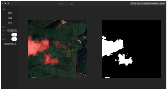
Figure 1.
CloudLabel v1.0 annotation software. The local left-side menu from top to bottom is: Undo, Enhance, Save, Growth Rate Settings, Fill, Eraser, and Update Default Configuration.
The construction of the Annotated Dataset for Training Cloud Segmentation (ADTCS) is used as an example to illustrate the CloudLabel annotation method. ADTCS, containing a total of 32,065 satellite cloud images of size 512 × 512, was created based on nine SPOT-6 satellite images [45]. The image is composed of three RGB channels with a fusion resolution of 1.5 m. The blue channel has a wavelength range from 0.455 to 0.525 μm, the green channel from 0.53 to 0.59 μm, and the red channel from 0.625 to 0.695 μm.
SPOT-6 is a satellite launched by the French Space Agency (CNES) in collaboration with Astrium GEO-Information Services, and represents the sixth generation of the SPOT series dedicated to Earth observation. Launched in 2012, SPOT-6 boasts the capability to deliver optical images with a high resolution of 1.5 m. This extensive coverage makes it invaluable for applications such as cartography, urban planning, agricultural monitoring, and disaster management. Together with its sister satellite, SPOT-7, SPOT-6 enhances the frequency of global coverage, providing timely data essential for environmental monitoring and emergency response management. Furthermore, SPOT-6 supports multispectral imaging, capturing information across various wavelengths, which is crucial for detailed analyses such as differentiating vegetation types and monitoring water bodies. The data from this satellite are widely used in both scientific research and commercial sectors, contributing significantly to environmental change monitoring, optimizing resource management, and enhancing Geographic Information System (GIS) applications. SPOT-6’s high-resolution imagery is particularly suited for urban and regional planning, offering high-quality geographic data support.
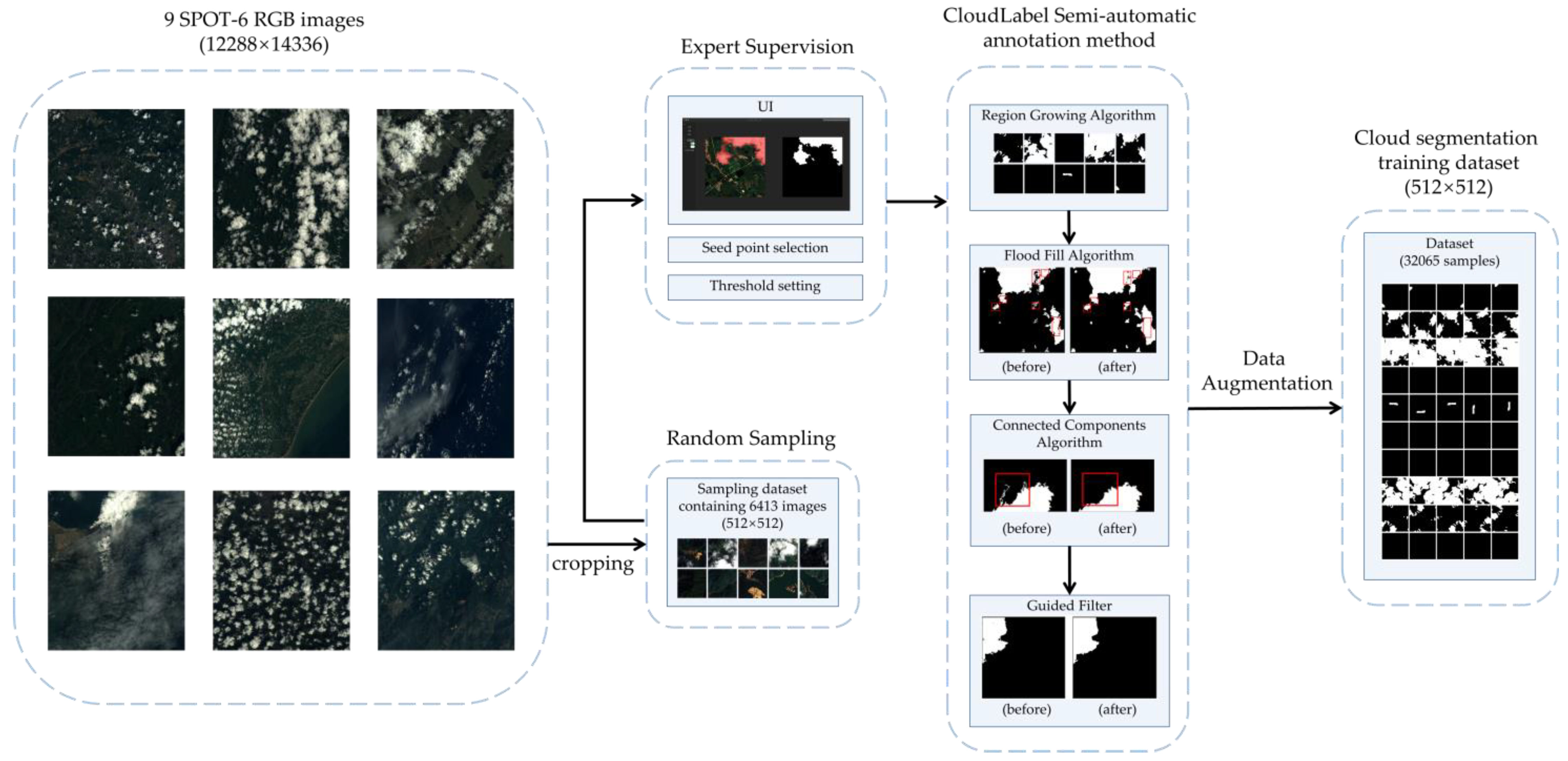
Ultimately, 6413 annotated images were obtained, and after data augmentation, ADTCS, containing 32,065 images of size 512 × 512 along with corresponding annotations, was generated. The construction process of ADTCS can be summarized in seven steps (Figure 2).
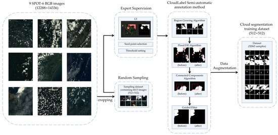
Figure 2.
ADTCS construction.
2.1. Step 1: Random Sampling
We first crop the 9 SPOT-6 images (12,288 × 14,336) into 6413 small images (512 × 512) by random sampling. In both the annotation and network training processes, coping with the excessive memory consumption of certain satellite image originals proves challenging. Therefore, after partitioning the dataset, it becomes necessary to crop the original images to a fixed size. If the cropped images are too large, an abundance of image information significantly increases the computational load of the model, leading to potential memory overflow. Conversely, if the cropped images are too small, insufficient feature information may hinder achieving satisfactory segmentation results. After multiple attempts, this dataset ultimately standardizes the sample size to 512 × 512, which is also widely used in previous excellent works on cloud segmentation [46,47,48] and dataset validation [29].
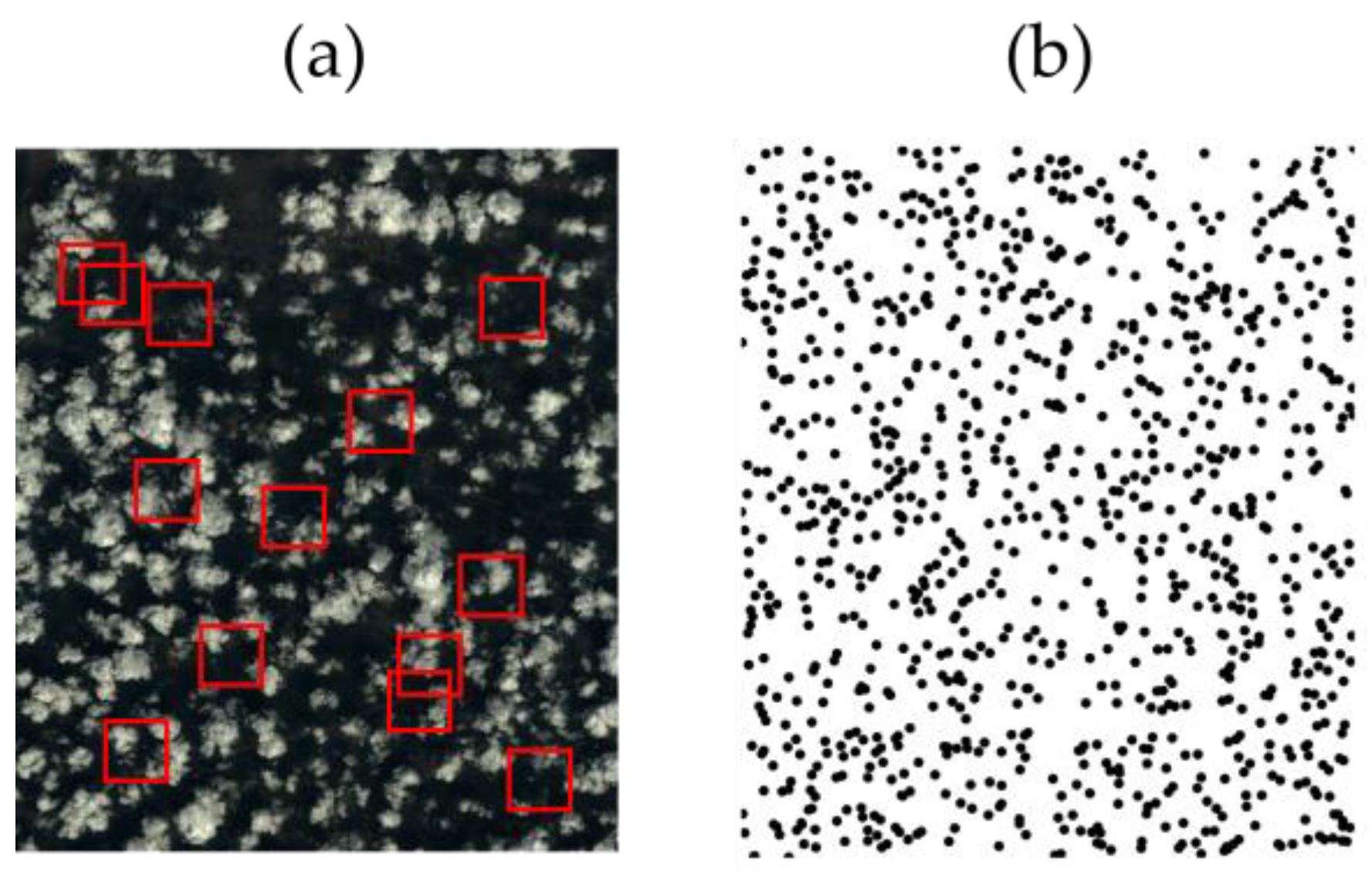
The sample selection typically employs three methods: regular grid selection, sliding window selection, and random selection. While the sliding window method ensures the comprehensive coverage of the image area, we found that it produces fewer samples in some cases, limiting the model’s learning potential. For example, a sliding window with fixed strides may generate only two samples from a given image, but with random sampling, we can obtain three to four samples from the same image. These additional samples from random sampling retain equivalent learning value because even partially overlapping images provide new, useful data for deep learning models. Random sampling introduces diversity by capturing more varied perspectives of the same region, thus enriching the dataset and contributing to better model generalization. Sliding window selection requires setting a stride size beforehand, followed by sliding a 512 × 512 window over the original image at the specified stride to select samples. While this method ensures sample richness, determining the optimal stride necessitates continuous trial and error based on the training effectiveness of the network model, which can be time- and resource-intensive. In contrast, the random selection method adopted by this dataset is more flexible and efficient. As illustrated in Figure 3, with this approach, 512 × 512-sized windows are randomly selected from the original image, and the number of samples can be manually defined. The abundance of samples effectively ensures randomness.
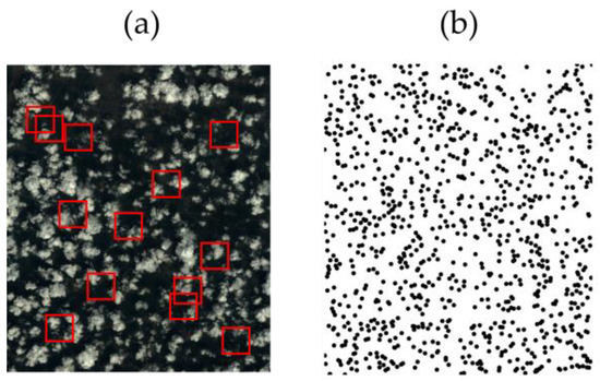
Figure 3.
Random sampling. (a) Demonstration of random window selection (red boxes). (b) Scatter plot of random selection (using a sample size of 1000 as an example).
The distribution of the dataset across 9 distinct satellite images ensures that users can easily avoid overlap between the training, validation, and test sets by selecting different images for each subset. This approach guarantees the independence of the test data, preserving its reference value and mitigating any concerns about overlap. By using distinct images for training, validation, and testing, users can ensure non-overlapping datasets.
The sample distribution across the dataset was determined based on the cloud coverage and variability present in each satellite image. A total of 32,065 images were extracted, with the number of samples per image as follows: wind10: 5000; wind11: 5000; wind12: 2500; wind1: 5000; wind22: 5000; wind27: 3360; wind36: 2640; wind41: 1130; and wind49: 2435. This distribution ensures a balance between data diversity and avoiding redundancy, with larger samples drawn from images exhibiting greater cloud variability. Although some overlap exists between cropped slices, CloudLabel’s semi-automatic annotation system, supported by region-growing and morphological algorithms, along with manual post-processing, ensures consistency across these overlapping regions. This approach minimizes noise while maintaining a sufficient number of samples for robust model training.
2.2. Step 2: Expert Supervision
In the second step, the segmented images are inputted into the UI interface of the CloudLabel annotation method for expert assessment. Experts determine the selection of seed points for region growing and set the threshold based on the details of cloud regions and specific conditions. In practical application, for bright, thick clouds, we often use pixels with moderately bright center brightness in the cloud region as seed points and set the threshold to T = 0.4; for darker, thinner cloud areas, the threshold is reduced to 0.2. Experts can further modify annotation details using tools such as erasers and magnifiers, and compare the masked image with the original image to ensure the reliability of the annotation results.
For ease of human–computer interaction, we have designed the CloudLabel annotation software, which integrates region growing, flood fill, connected components and guided filtering techniques from step 3 to step 6 (see Figure 1). The usage method is as follows: input the address of the cloud image to be annotated in the search bar at the top right corner to open the image. Then, set an appropriate growth rate in the taskbar on the left side. Click on any pixel within the cloud-containing area to annotate the surrounding region. Once the basic annotation of cloud regions is completed, click on the “Enhance” button in the taskbar on the left to perform morphological processing for optimizing the results. Therefore, with CloudLabel, the experts only need to manually select the starting point for region growing and set the growth rate to semi-automatically annotate high spatial resolution satellite images.
Our annotation process was designed with specific measures to mitigate the noise introduced by inconsistency between slices. Firstly, the cropping is performed on high-resolution images, and overlapping regions between slices are minimal. Furthermore, CloudLabel, the semi-automatic annotation tool we employed, uses advanced region-growing and morphological algorithms (such as flood fill and connected components), which are designed to maintain spatial coherence across contiguous regions. This minimizes discrepancies in annotation between overlapping areas. Additionally, we conducted manual post-processing to review and correct any inconsistencies that might arise between slices. This ensures that the same target is consistently annotated across overlapping regions, reducing the potential for noise caused by misaligned annotations.
2.3. Step 3: Region Growing Algorithm
CloudLabel primarily relies on region growing [42,43], coupled with morphological processing to modify the edges of cloud regions, employing a semi-automatic annotation approach for cloud regions in high-spatial-resolution remote sensing images through human–computer interaction.
Region growing is a technique used to segment an image based on the similarity of pixel properties. The method starts with an initial seed point and iteratively adds neighboring pixels to the region if they meet certain criteria, typically based on intensity or color similarity. The key components of region growing include seed point selection, growth criteria definition, and threshold setting. In our work, the process continues until the region stops expanding, when the difference between neighboring pixels exceeds a gray level threshold supervised by experts. By appropriately selecting these parameters, region growing can effectively partition an image into coherent regions with similar properties. For instance, assuming the grayscale distribution of the original matrix is , the region growing results with a threshold of 1 are depicted as , while the region growing results with a threshold of 3 are depicted as :
2.4. Step 4: Flood Fill Algorithm
In contrast to medium-to-low-resolution remote sensing images, high-spatial-resolution remote sensing images exhibit detailed terrain features, with significant variations in grayscale values within cloud regions. Some pixels within these regions may have much higher or lower values than their surrounding pixels. Consequently, when employing region growing alone, excessively dark or bright pixels within cloud regions may not be properly identified, resulting in the formation of holes. Therefore, in this project, we utilize the flood fill algorithm from morphological image processing to fill in the coarse results obtained from region growing for cloud annotation. As depicted in Figure 4, although the coarse cloud annotation results already provide rough outlines, the pixels within the red box remain black, indicating that the pixels at corresponding positions in the original image were not recognized by the region growing method. After performing hole filling operations, these pixels turn white.

Figure 4.
Schematic representation of hole filling. (a) Original image, (b) original labelling mask of region growing algorithm after step 3, (c) before hole filling, and (d) after hole filling.
2.5. Step 5: Connected Components Algorithm
The region growing method relies on superficial features of pixels in the image—grayscale values. However, it can lead to misclassification when encountering man-made objects (buildings, roads, etc.) with high reflectance similar to clouds. Nevertheless, in high-spatial-resolution remote sensing images, clouds typically exhibit natural and random shapes, with overall roundedness and smooth edges. Conversely, man-made structures often possess regular shapes such as linear, rectangular, or circular patterns. Therefore, these man-made objects can be removed based on their characteristic regular shapes. The specific method is outlined below.
Utilizing the connected-component method, the annotation results obtained from region growing are partitioned into distinct connected regions. The number of pixels contained within each connected region, denoted as , is calculated, along with determining the minimum bounding rectangle for each connected region. Denoting the number of pixels contained within the minimum bounding rectangle as , the ratio between and is computed:
By analyzing the ratio , man-made objects with regular shapes can be distinguished and removed from the cloud annotation results.
If , it indicates that the connected region is approximately rectangular; if , the connected region is approximately circular; if , the connected region is approximately linear. Therefore, by selecting an appropriate range and satisfying the above conditions, all pixels within the connected region are assigned a value of 0, effectively removing man-made objects with high reflectance.
Cloud targets are inherently irregular. Therefore, when satisfies the aforementioned three conditions, it indicates that the target is overly regular, likely indicating a man-made object. For example, in the illustration below (see Figure 5), there is a clear case where the region growing method mistakenly identifies roads as clouds. Consequently, after applying the connected-component labeling method for removal, the road targets are corrected. Of course, there are rare cases where cloud targets also exhibit regular shapes. However, the correction process is supervised by experts, ensuring timely rectification in such cases.

Figure 5.
Connected components algorithm result. (a) original image, (b) before rectification, and (c) after rectification.
2.6. Step 6: Guided Filter
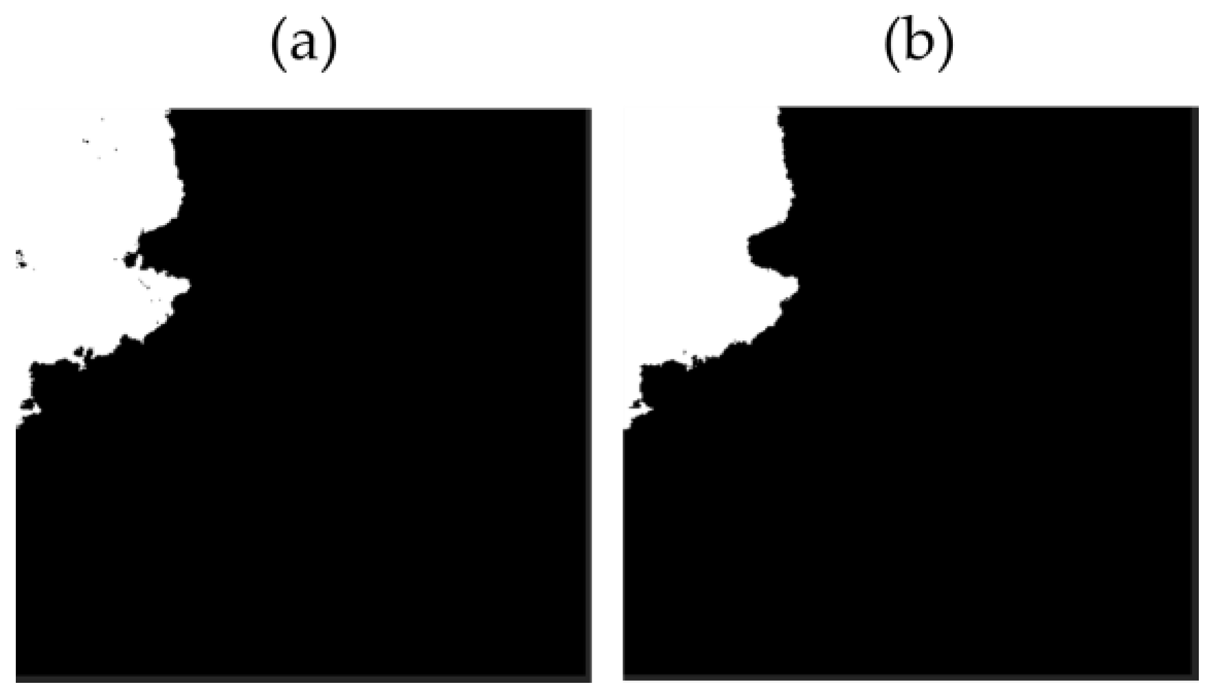
In high-spatial-resolution remote sensing images, the boundaries of cloud regions often appear as blurry, semi-transparent pixels. These edge areas have reflectance similar to that of the terrain, unlike the pixels in the center of the cloud region, which exhibit high reflectance. Consequently, they are prone to misclassification. To address this issue, this project utilizes guided filtering for the fine segmentation of the coarse annotation results, thereby improving the characteristics of cloud region boundaries. The formula is as follows:
where represents the guided filter, represents the coarse annotation results of the cloud region, the satellite image is considered as the guidance image, is the window radius of the guided filter, and is the regularization parameter of the guided filter. A comparison before and after guided filtering is shown in Figure 6 below, in which the edges of the cloud regions have become reasonably smoother.
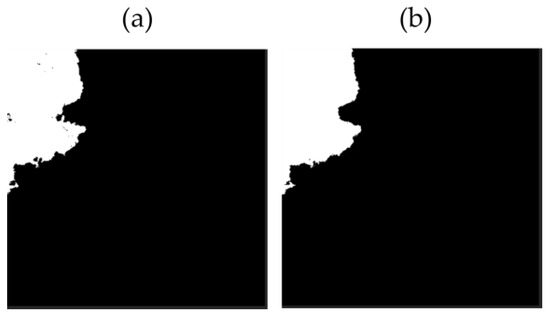
Figure 6.
Guided filter result. (a) Labeling mask after step 5, and (b) after guided filtering.
2.7. Step 7: Data Augmentation
After obtaining labeling results of the 6413 small images, a pivotal strategy involvea harnessing the power of data augmentation methods to enrich the annotated dataset. Through a judicious application of mirroring and rotation techniques, the initial pool of 6413 labeled images is substantially augmented, expanding the dataset to a robust compilation of 32065 images. This augmentation not only bolsters the dataset’s size but also diversifies its content, enhancing its utility and enabling more comprehensive training and analysis. However, some deep learning-based models use rotation and flipping to perform data enhancement on the code side rather than directly generating redundant data. Consequently, during the data augmentation process, each original image is assigned a suffix of ‘_0’, and its four augmented counterparts are assigned suffixes ‘_1’ through ‘_4’. The remaining portions of the filenames remain consistent across these versions. This labeling strategy allows users to easily identify and select whether to include augmented data based on their specific research needs.
3. Results
3.1. General Description
In the realm of meteorological research, accurate cloud segmentation is pivotal for enhancing weather prediction models and understanding atmospheric processes. Traditional manual labeling methods are time-intensive and subject to human error, particularly when distinguishing subtle cloud features or thin cloud formations. To address these challenges, we have developed a semi-automatic labeling tool, CloudLabel, designed to streamline the creation of high-quality datasets for training deep learning models in cloud segmentation tasks.
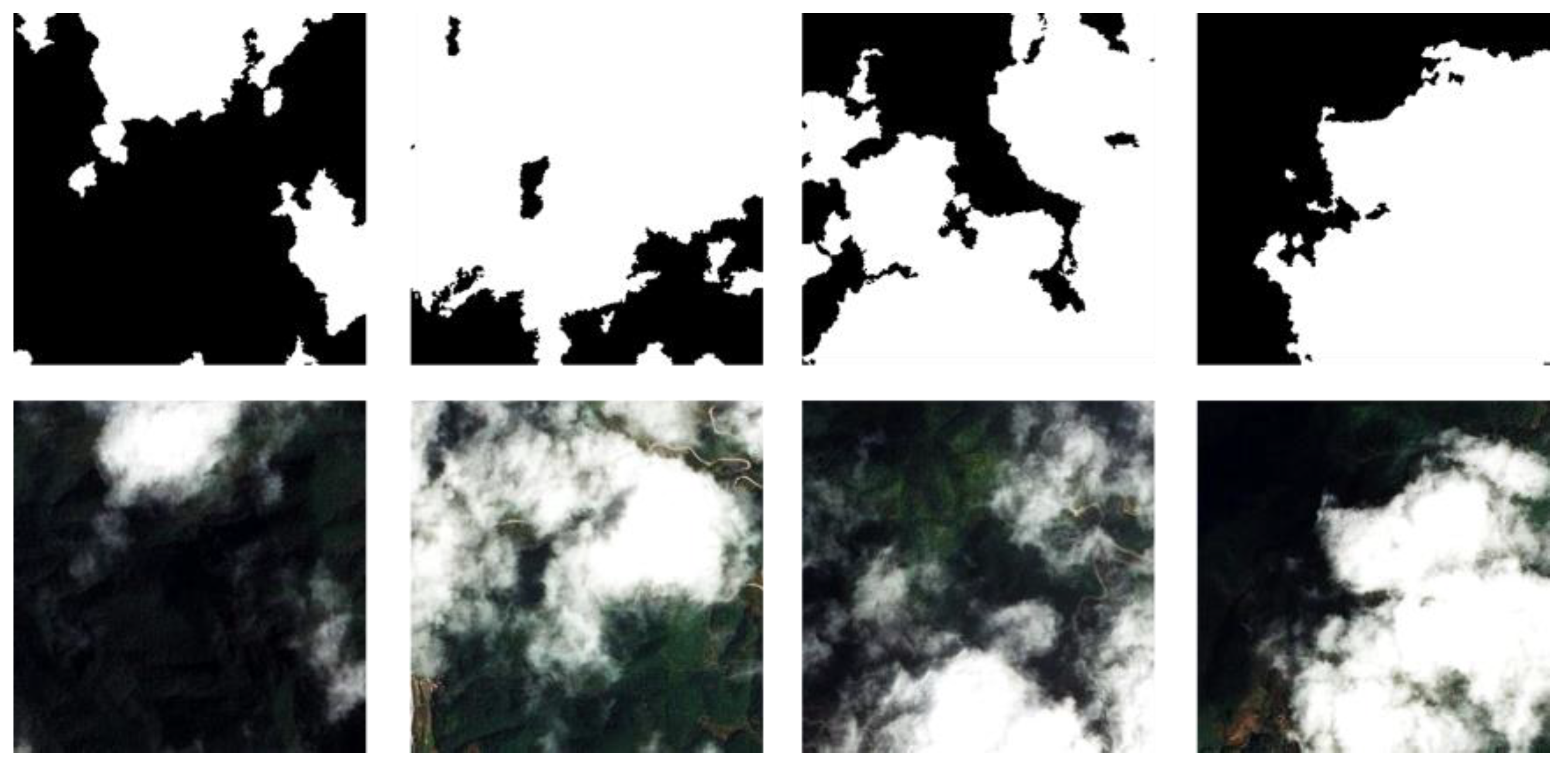
CloudLabel employs a combination of edge detection techniques and morphological analysis to enhance the precision of the segmentation process. As shown in Figure 7, this approach not only retains the intricate details of cloud edges and features but also accurately classifies difficult-to-label phenomena such as cirrus or thin clouds, which are often overlooked using conventional methods. Furthermore, CloudLabel incorporates advanced filtering algorithms to reduce the misclassification of non-cloud elements like roads or houses, a common issue in many cloud detection systems. By refining the accuracy of cloud delineation, our method substantially diminishes the risk of incorporating erroneous data into the training sets, which could potentially skew the model’s performance.
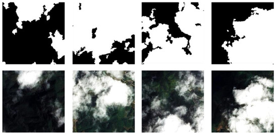
Figure 7.
CloudLabel results: (up) labeling results; (down) corresponding original RGB images.
In our dataset comprising 32,065 samples, the number of images with various cloud coverage rates is relatively uniform (Figure 8). Remarkably, over 13,000 samples exhibit a cloud coverage of less than 2%, while a substantial cohort of more than 5000 samples presents a cloud coverage exceeding 98%. The remaining 14,000-plus samples showcase a relatively uniform distribution of cloud coverage. This diverse array of cloud coverages offers a fertile ground for advancing cloud segmentation deep learning methodologies.
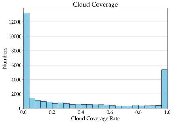
Figure 8.
Cloud coverage distribution.
The prevalence of samples with extremely low and high cloud coverage percentages provides a rich reservoir for training deep learning models. Samples with minimal cloud coverage facilitate the extraction of characteristics of underlying surface and artificial features, while those with high cloud coverage offer a nuanced understanding of complex cloud formations. Moreover, the presence of samples with varying degrees of cloud coverage enables the development of robust algorithms capable of accurately delineating clouds under diverse conditions.
Remote sensing satellite imagery provides valuable insights into the Earth’s surface and atmospheric phenomena. Understanding the complexity of surface features and cloud formations in these images is crucial for various applications such as weather forecasting and environmental monitoring. In this study, we used the image information entropy, denoted as , to measure the randomness or uncertainty present in an image. It is calculated based on the probability distribution of pixel intensities within the image. For a grayscale image, the formula for image information entropy is given by:
where is the number of possible intensity levels (here, 256 for an 8-bit grayscale image), and is the probability of occurrence of intensity level in the image. To assess the complexity of surface features and cloud formations in remote sensing satellite imagery, we apply the image information entropy calculation. A higher value of image information entropy indicates greater complexity and variability in the pixel intensities, suggesting a more intricate surface terrain or cloud structure. Conversely, a lower entropy value suggests a more uniform or homogeneous appearance.
By quantifying the complexity of surface features and cloud formations in remote sensing satellite imagery using image information entropy, our method provides a valuable tool for analyzing and interpreting satellite data for diverse applications in atmospheric and environmental sciences. This approach enables researchers to gain a general understanding of the complexity of images in dataset.
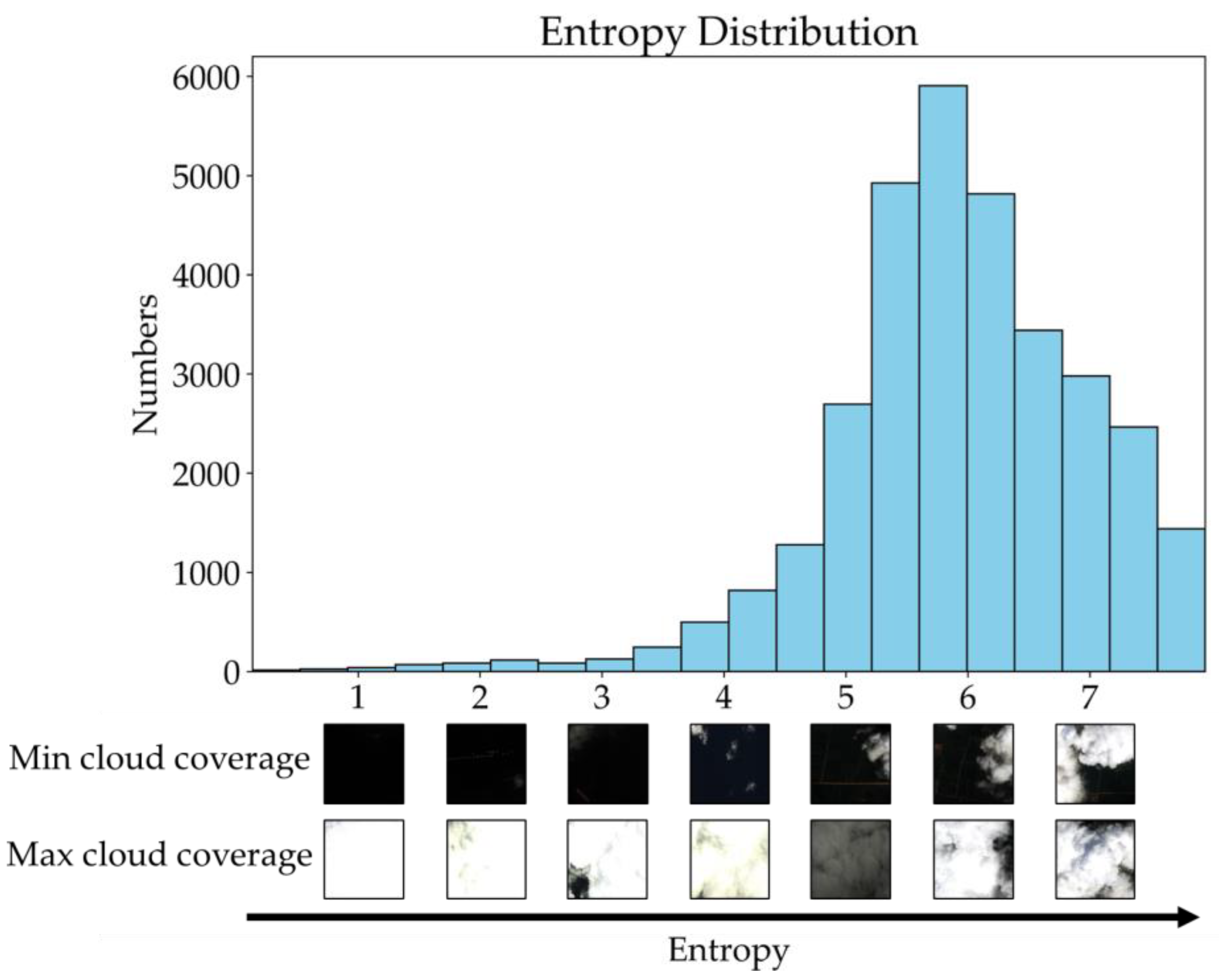
As depicted in Figure 9, the distribution of image entropy within our dataset reveals a concentration of values ranging from 5 to 7, indicating a high degree of image complexity. This richness in sample information is crucial for training neural networks, as it allows them to learn a more comprehensive set of features, enhancing their predictive accuracy and robustness in practical applications.

Figure 9.
Image entropy distribution of the dataset. The max and min cloud coverage image of each entropy are shown at the bottom.
The relationship between image entropy and cloud coverage is not directly proportional, as Figure 9 illustrates. The simplest images (with the lowest entropy) often represent clear skies or completely cloud-covered scenes. These scenarios present minimal variability and lower informational content, which, while less challenging for segmentation algorithms, offer limited learning opportunities for complex feature extraction.
Conversely, the most complex images (with the highest entropy) generally depict mixed scenes where clouds and land features are interspersed with high variability. These images encapsulate a wealth of features, including varying textures, gradients, and structural details, making them ideal for training advanced neural network models. The richness of these samples provides a dynamic learning environment where the model can effectively differentiate between nuanced atmospheric phenomena and terrestrial elements. By leveraging such detailed datasets, researchers can significantly improve the predictive capabilities of deep learning models, contributing to more accurate cloud segmentation.
3.2. Advantage of the CloudLabel Semi-Automatic Labeling Method
Here, we have selected LabelMe [40], a distinguished annotation tool widely utilized in the field of computer vision, for comparison. Despite its general utility, the unique characteristics of cloud targets, such as their loose structure and highly irregular edges, necessitate tailored algorithms to optimize annotation results. The polygonal annotation method employed by LabelMe often falls short of capturing the intricate details of cloud regions. Consequently, we will conduct a comparative analysis of cloud segmentation annotations between LabelMe and our specialized cloud-targeted tool, CloudLabel, to highlight the enhancements our approach offers in detailing cloud features.
Figure 10 presents a comparative analysis of cloud annotation results using LabelMe and our novel CloudLabel method. On the one hand, the LabelMe annotations exhibit overly smoothed cloud boundaries as a result of the software’s inherent post-processing features, which can obscure important textural details critical for accurate cloud segmentation. In contrast, CloudLabel retains the intricate edge details present in high-resolution remote sensing imagery, capturing a richer array of texture characteristics that are vital for precise cloud identification.

Figure 10.
Comparison of the labeling results of LabelMe (b) and CloudLabel (c) based on the same RGB image (a).
Furthermore, the cloud areas annotated with LabelMe rely heavily on manual delineation, introducing a degree of subjectivity that may lead to inconsistent labeling across different annotators. CloudLabel, on the other hand, employs image processing techniques such as region growing methods that objectively differentiate between clouded and clear areas based on pixel values. This approach minimizes the subjective errors inherent in human observation and judgment, reducing the potential for misclassification.
3.3. Performance of Widely Used Cloud Segmentation Algorithms on the Dataset (Underlying Surfaces of Forest Areas)
We conducted experiments using several well-known neural network models, including UNet, CDNet, DANet, ResNet, DeeplabV3, and DeeplabV3Plus. These models were trained on the ADTCS dataset, and to ensure a robust evaluation, we tested their performance using independent SPOT-6 satellite images that were not included in the dataset. This approach enabled us to validate the generalization capability of the models and assess their effectiveness in cloud segmentation tasks.
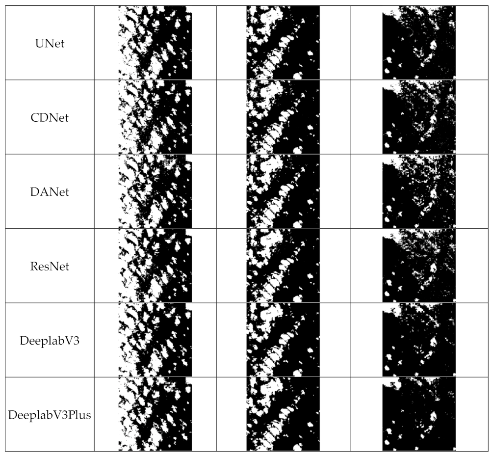
Figure 11 results show that in remote sensing satellite images with forest as the underlying surface, where the environment predominantly consists of dark-colored trees, there are numerous false detections when using models such as UNet, CDNet, DANet, ResNet, DeeplabV3, and DeeplabV3Plus for the segmentation of these images.
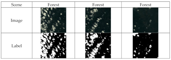
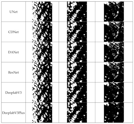
Figure 11.
Cloud segmentation results in forest scenes after training with the ADTCS dataset for different models.
In forest scenes, as shown in Table 1, ResNet performed the worst, with an IoU of only 63.32%, an OA of 88.19%, and an F1 score of 77.54%. UNet, CDNet, and DANet achieved moderate overall performance, with IoU values around 75%, OA around 94%, and F1 scores around 86%. These models effectively segmented the main cloud bodies but exhibited false detections at the cloud edges, which negatively impacted the overall metrics. DeepLabv3 and DeepLabv3Plus demonstrated better overall performance, with IoU around 80% and OA around 95%, and were able to segment the clouds more accurately, capturing richer boundary texture information.

Table 1.
Cloud segmentation results in forest scenes after training with the ADTCS dataset for different models.
3.4. Performance of Widely Used Cloud Segmentation Algorithms on the Dataset (Underlying Surfaces of Island Areas)
In addition to the forest scenes, we also tested satellite images in island scenes.
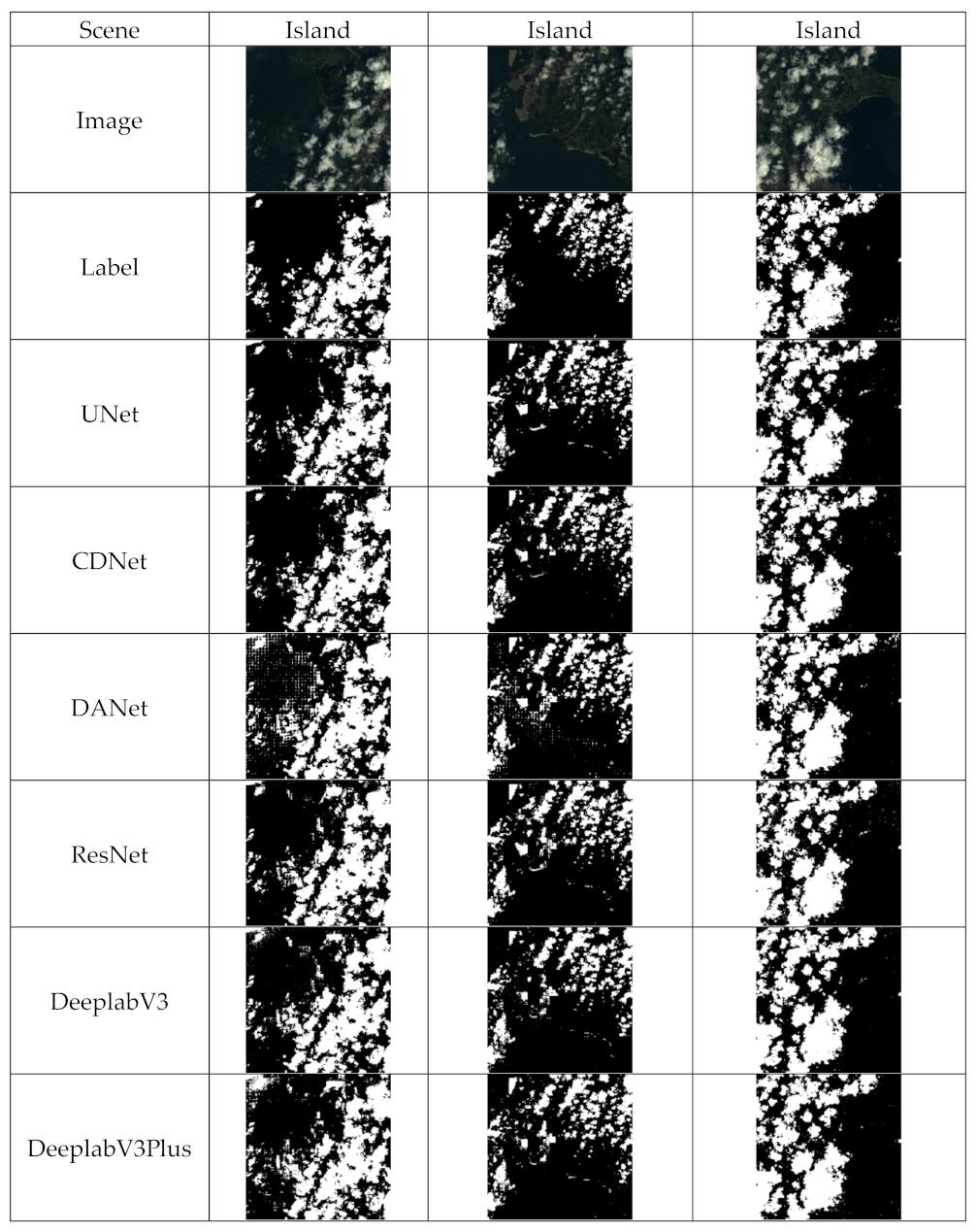
Figure 12 shows that in remote sensing satellite images of islands, the underlying surface is quite complex, including various geographical features such as oceans, land, roads, and buildings. When using models such as Unet, CDNet, ResNet, FFDANet, DeepLabv3, and DeepLabv3Plus to segment these images, the main cloud areas can be accurately identified.

Figure 12.
Cloud segmentation results in island scenes after training with the ADTCS dataset for different models.
In island scenes, as shown in Table 2, Unet, DANet, ResNet, and Deeplabv3 exhibit moderate overall performance. While they can effectively segment the main cloud regions, false detections occur at the cloud edges, which negatively impact the overall metrics. DeepLabv3 and DeepLabv3Plus perform better overall, with IoU around 80% and OA around 95%.

Table 2.
Cloud segmentation results in island scenes after training with the ADTCS dataset for different models.
4. Discussion
The dataset constructed using the CloudLabel approach not only provides a robust foundation for training deep learning models but also introduces a paradigm shift in how we approach cloud segmentation tasks. These models are expected to exhibit superior performance, thanks to the high-quality, accurately labeled training data. The CloudLabel method’s effectiveness in retaining intricate edge details and rich texture characteristics, as demonstrated in the comparative analysis with LabelMe, enhances its utility in creating highly detailed annotations that are essential for advanced neural network training.
Furthermore, the semi-automatic nature of CloudLabel combines the precision of manual annotation with the efficiency of automated algorithms, significantly reducing the time and labor typically required for such detailed annotation tasks. By addressing both the edge complexity and the varied texture of cloud formations, CloudLabel facilitates a more nuanced feature extraction process, enabling neural networks to develop a more refined understanding of cloud and non-cloud distinctions.
The integration of datasets annotated with CloudLabel into deep learning network models enables these models to effectively replicate small-scale cloud features, crucial for achieving pixel-level accuracy in cloud segmentation tasks. This capability is vital for enhancing meteorological research, improving weather forecasting accuracy, and enriching our understanding of atmospheric processes. The precise delineation of cloud boundaries informed by the detailed and rich dataset contributes to more accurate climate models and forecasts.
In practical terms, the CloudLabel annotated cloud segmentation training dataset has shown potential for broader applications in remote sensing. Its capacity to handle complex cloud segmentation scenarios, where cloud patterns and formations vary greatly, makes it a valuable resource for advancing cloud classification techniques. The insights gained from this dataset could significantly impact weather forecasting, climate monitoring, and atmospheric science research, potentially leading to more informed environmental policies and strategies.
Future studies may explore the integration of additional atmospheric variables and enhanced image processing algorithms to further refine the accuracy and reliability of cloud segmentation. Moreover, the scalability of CloudLabel could be tested in other remote sensing applications, potentially broadening its utility beyond cloud segmentation. Ultimately, the continued development and refinement of tools like CloudLabel are pivotal for advancing the capabilities of remote sensing technologies and for providing more accurate, actionable insights into the ever-changing dynamics of atmosphere.
5. Conclusions
In conclusion, the introduction of the CloudLabel semi-automatic annotation tool marks significant progress in the annotation of high-resolution satellite imagery for cloud segmentation. This tool addresses the challenges inherent in accurately distinguishing cloud from non-cloud regions by implementing a sophisticated blend of region growing and morphological processing techniques. The resultant dataset, consisting of 32,065 RGB images with 1.5 m resolution and corresponding high-quality CloudLabel labeling results, not only augments the depth of training data available for deep learning models but also enhances the overall efficacy of these models in real-world remote sensing applications.
In future work, it is meaningful to integrate advanced segmentation models, such as the Segment Anything Model (SAM) [49], into the preprocessing method. SAM’s general-purpose segmentation capabilities could automate initial segmentation tasks and subsequently refine the annotations using our proposed method. This approach has the potential to significantly improve the efficiency and scalability of workflow, making it more suitable for large-scale datasets.
Author Contributions
Conceptualization, J.Z. and X.Z.; methodology, X.Z.; software, X.Z.; validation, J.Z. and M.H.; formal analysis, J.Z.; investigation, Z.G. and Y.H.; resources, Z.G. and Y.H.; data curation, X.Z.; writing—original draft preparation, J.Z.; writing—review and editing, J.Z.; visualization, J.Z.; supervision, M.H.; project administration, M.H.; funding acquisition, M.H. All authors have read and agreed to the published version of the manuscript.
Funding
This research received no external funding.
Data Availability Statement
The annotated dataset files for training cloud segmentation neural net-works using high-resolution satellite remote sensing imagery for each grid point are freely available for download at the Science Data Bank, with the following link: https://www.scidb.cn/en/s/yQZ77f (accessed on 1 October 2024).
Conflicts of Interest
The authors declare no conflicts of interest.
References
- Irons, J.R.; Dwyer, J.L.; Barsi, J.A. The next Landsat satellite: The Landsat Data Continuity Mission. Remote Sens. Environ. 2012, 122, 11–21. [Google Scholar] [CrossRef]
- Loveland, T.R.; Dwyer, J.L. Landsat: Building a strong future. Remote Sens. Environ. 2012, 122, 22–29. [Google Scholar] [CrossRef]
- Jutz, S.; Milagro-Perez, M.P. Copernicus: The European Earth Observation programme. Rev. De Teledetección 2020, 56, V–XI. [Google Scholar] [CrossRef]
- Bai, C.; Zhang, M.; Zhang, J.; Zheng, J.; Chen, S. LSCIDMR: Large-scale satellite cloud image database for meteorological research. IEEE Trans. Cybern. 2021, 52, 12538–12550. [Google Scholar] [CrossRef]
- Fu, Y.; Mi, X.; Han, Z.; Zhang, W.; Liu, Q.; Gu, X.; Yu, T. A Machine-Learning-Based Study on All-Day Cloud Classification Using Himawari-8 Infrared Data. Remote Sens. 2023, 15, 5630. [Google Scholar] [CrossRef]
- Hang, R.; Wang, J.; Ge, L.; Shi, C.; Wei, J. Convective Cloud Detection From Himawari-8 Advanced Himawari Imager Data Using a Dual-Branch Deformable Convolutional Network. IEEE J. Sel. Top. Appl. Earth Obs. Remote Sens. 2024, 17, 7490–7500. [Google Scholar] [CrossRef]
- Zheng, K.; Li, J.; Yang, J.; Ouyang, W.; Wang, G.; Zhang, X. A cloud and snow detection method of TH-1 image based on combined ResNet and DeeplabV3+. Acta Geod. Et Cartogr. Sin. 2020, 49, 1343. [Google Scholar]
- Lee, Y.; Kummerow, C.D.; Ebert-Uphoff, I. Applying machine learning methods to detect convection using GOES-16 ABI data. Atmos. Meas. Techn. Discuss 2020, 2020, 1–28. [Google Scholar]
- Li, W.; Zhang, F.; Lin, H.; Chen, X.; Li, J.; Han, W. Cloud detection and classification algorithms for Himawari-8 imager measurements based on deep learning. IEEE Trans. Geosci. Remote Sens. 2022, 60, 1–17. [Google Scholar] [CrossRef]
- Jeppesen, J.H.; Jacobsen, R.H.; Inceoglu, F.; Toftegaard, T.S. A cloud detection algorithm for satellite imagery based on deep learning. Remote Sens. Environ. 2019, 229, 247–259. [Google Scholar] [CrossRef]
- Li, Z.; Shen, H.; Cheng, Q.; Liu, Y.; You, S.; He, Z. Deep learning based cloud detection for medium and high resolution remote sensing images of different sensors. ISPRS J. Photogramm. Remote Sens. 2019, 150, 197–212. [Google Scholar] [CrossRef]
- Parente, L.; Taquary, E.; Silva, A.P.; Souza, C.; Ferreira, L. Next Generation Mapping: Combining Deep Learning, Cloud Computing, and Big Remote Sensing Data. Remote Sens. 2019, 11, 2881. [Google Scholar] [CrossRef]
- Yuan, X.; Shi, J.; Gu, L. A review of deep learning methods for semantic segmentation of remote sensing imagery. Expert Syst. Appl. 2021, 169, 114417. [Google Scholar] [CrossRef]
- Ge, W.; Yang, X.; Jiang, R.; Shao, W.; Zhang, L. CD-CTFM: A Lightweight CNN-Transformer Network for Remote Sensing Cloud Detection Fusing Multiscale Features. J. Sel. Top. Appl. Earth Obs. Remote Sens. 2024, 17, 4538–4551. [Google Scholar] [CrossRef]
- Liu, Q.; Li, Y.; Yu, M.; Chiu, L.S.; Hao, X.; Duffy, D.Q.; Yang, C. Daytime rainy cloud detection and convective precipitation delineation based on a deep neural Network method using GOES-16 ABI images. Remote Sens. 2019, 11, 2555. [Google Scholar] [CrossRef]
- Ukkonen, P.; Mäkelä, A. Evaluation of machine learning classifiers for predicting deep convection. Adv. Model. Earth Syst. 2019, 11, 1784–1802. [Google Scholar] [CrossRef]
- Zhang, M.; Li, W.; Du, Q. Diverse region-based CNN for hyperspectral image classification. IEEE Trans. Image Process. 2018, 27, 2623–2634. [Google Scholar] [CrossRef]
- Xiao, C.; Sun, J. Deep Neural Networks (DNN). In Introduction to Deep Learning for Healthcare; Xiao, C., Sun, J., Eds.; Springer International Publishing: Cham, Switzerland, 2021; pp. 41–61. [Google Scholar]
- Francis, A.; Sidiropoulos, P.; Muller, J.-P. CloudFCN: Accurate and robust cloud detection for satellite imagery with deep learning. Remote Sens. 2019, 11, 2312. [Google Scholar] [CrossRef]
- Redmon, J.; Divvala, S.; Girshick, R.; Farhadi, A. You Only Look Once: Unified, Real-Time Object Detection. In Proceedings of the IEEE Conference on Computer Vision and Pattern Recognition 2016, Las Vegas, NV, USA, 27–30 June 2016; pp. 779–788. [Google Scholar]
- Jin, X.; He, J.; Xiao, Y.; Lihe, Z.; Liao, X.; Li, J.; Yuan, Q. RFE-VCR: Reference-enhanced transformer for remote sensing video cloud removal. Photogramm. Remote Sens. 2024, 214, 179–192. [Google Scholar] [CrossRef]
- Sui, J.; Ma, Y.; Yang, W.; Zhang, X.; Pun, M.-O.; Liu, J. Diffusion Enhancement for Cloud Removal in Ultra-Resolution Remote Sensing Imagery. IEEE Trans. Geosci. Remote Sens. 2024, 62, 1–14. [Google Scholar] [CrossRef]
- He, M.; Zhang, J. Radiation Feature Fusion Dual-Attention Cloud Segmentation Network. Remote Sens. 2024, 16, 2025. [Google Scholar] [CrossRef]
- Zhang, J.; He, M. Methodology for Severe Convective Cloud Identification Using Lightweight Neural Network Model Ensembling. Remote Sens. 2024, 16, 2070. [Google Scholar] [CrossRef]
- Song, Q.; Cui, Z.; Liu, P. An Efficient Solution for Semantic Segmentation of Three Ground-based Cloud Datasets. Earth Space Sci. 2020, 7, e2019EA001040. [Google Scholar] [CrossRef]
- Mohajerani, S.; Saeedi, P. Cloud-Net: An End-To-End Cloud Detection Algorithm for Landsat 8 Imagery. In Proceedings of the IGARSS 2019—2019 IEEE International Geoscience and Remote Sensing Symposium, Yokohama, Japan, 28 July–2 August 2019; pp. 1029–1032. [Google Scholar]
- Foga, S.; Scaramuzza, P.L.; Guo, S.; Zhu, Z.; Dilley, R.D., Jr.; Beckmann, T.; Schmidt, G.L.; Dwyer, J.L.; Hughes, M.J.; Laue, B. Cloud detection algorithm comparison and validation for operational Landsat data products. Remote Sens. Environ. 2017, 194, 379–390. [Google Scholar] [CrossRef]
- Hughes, M.J.; Hayes, D.J. Automated detection of cloud and cloud shadow in single-date Landsat imagery using neural networks and spatial post-processing. Remote Sens. 2014, 6, 4907–4926. [Google Scholar] [CrossRef]
- Aybar, C.; Ysuhuaylas, L.; Loja, J.; Gonzales, K.; Herrera, F.; Bautista, L.; Yali, R.; Flores, A.; Diaz, L.; Cuenca, N.; et al. CloudSEN12, a global dataset for semantic understanding of cloud and cloud shadow in Sentinel-2. Sci. Data 2022, 9, 782. [Google Scholar] [CrossRef]
- Chen, Q.; Yin, X.; Li, Y.; Zheng, P.; Chen, M.; Xu, Q. Recognition of Severe Convective Cloud Based on the Cloud Image Prediction Sequence from FY-4A. Remote Sens. 2023, 15, 4612. [Google Scholar] [CrossRef]
- Gong, C.; Long, T.; Yin, R.; Jiao, W.; Wang, G. A Hybrid Algorithm with Swin Transformer and Convolution for Cloud Detection. Remote Sens. 2023, 15, 5264. [Google Scholar] [CrossRef]
- Li, T.; Wu, D.; Wang, L.; Yu, X. Recognition algorithm for deep convective clouds based on FY4A. Neural Comput. Appl. 2022, 34, 21067–21088. [Google Scholar] [CrossRef]
- Tian, Y.; Pang, S.; Qu, Y. Fusion Cloud Detection of Multiple Network Models Based on Hard Voting Strategy. In Proceedings of the IGARSS 2022—2022 IEEE International Geoscience and Remote Sensing Symposium, Kuala Lumpur, Malaysia, 17–22 July 2022; pp. 6646–6649. [Google Scholar]
- Luotamo, M.; Metsämäki, S.; Klami, A. Multiscale cloud detection in remote sensing images using a dual convolutional neural network. IEEE Trans. Geosci. Remote Sens. 2020, 59, 4972–4983. [Google Scholar] [CrossRef]
- Hu, K.; Zhang, D.; Xia, M.; Qian, M.; Chen, B. LCDNet: Light-weighted cloud detection network for high-resolution remote sensing images. IEEE J. Sel. Top. Appl. Earth Obs. Remote Sens. 2022, 15, 4809–4823. [Google Scholar] [CrossRef]
- Li, Y.; Chen, W.; Zhang, Y.; Tao, C.; Xiao, R.; Tan, Y. Accurate cloud detection in high-resolution remote sensing imagery by weakly supervised deep learning. Remote Sens. Environ. 2020, 250, 112045. [Google Scholar] [CrossRef]
- Wu, Z.; Li, J.; Wang, Y.; Hu, Z.; Molinier, M. Self-attentive generative adversarial network for cloud detection in high resolution remote sensing images. IEEE Geosci. Remote Sens. Lett. 2019, 17, 1792–1796. [Google Scholar] [CrossRef]
- Zhang, G.; Gao, X.; Yang, J.; Yang, Y.; Tan, M.; Xu, J.; Wang, Y. A multi-task driven and reconfigurable network for cloud detection in cloud-snow coexistence regions from very-high-resolution remote sensing images. Int. J. Appl. Earth Obs. Geoinf. 2022, 114, 103070. [Google Scholar] [CrossRef]
- See, L.; Sturn, T.; Karanam, S.; Subash, A.; McCallum, I.; Fritz, S. Combining a rapid image classification app with artificial intelligence through the Picture Pile Platform for citizen science. In Proceedings of the ECSA Conference, Berlin, Germany, 5–7 October 2022. [Google Scholar]
- Russell, B.C.; Torralba, A.; Murphy, K.P.; Freeman, W.T. LabelMe: A database and web-based tool for image annotation. Int. J. Comput. Vis. 2008, 77, 157–173. [Google Scholar] [CrossRef]
- Drusch, M.; Del Bello, U.; Carlier, S.; Colin, O.; Fernandez, V.; Gascon, F.; Hoersch, B.; Isola, C.; Laberinti, P.; Martimort, P. Sentinel-2: ESA’s optical high-resolution mission for GMES operational services. Remote Sens. Environ. 2012, 120, 25–36. [Google Scholar] [CrossRef]
- Otto, G.P.; Chau, T.K. ‘Region-growing’algorithm for matching of terrain images. Image Vis. Comput. 1989, 7, 83–94. [Google Scholar] [CrossRef]
- Tang, J. A color image segmentation algorithm based on region growing. In Proceedings of the 2010 2nd International Conference on Computer Engineering and Technology, Chengdu, China, 16–18 April 2010; pp. V6-634–V636-637. [Google Scholar]
- Chevrel, M.; Courtois, M.; Weill, G. The SPOT satellite remote sensing mission. Photogramm. Eng. Remote Sens. 1981, 47, 1163–1171. [Google Scholar]
- Cheng, P. SPOT-6 and SPOT-7 Satellites. GeoInformatics 2015, 18, 24. [Google Scholar]
- Chai, D.; Newsam, S.; Zhang, H.K.; Qiu, Y.; Huang, J. Cloud and cloud shadow detection in Landsat imagery based on deep convolutional neural networks. Remote Sens. Environ. 2019, 225, 307–316. [Google Scholar] [CrossRef]
- Zhang, H.K.; Luo, D.; Roy, D.P. Improved Landsat Operational Land Imager (OLI) Cloud and Shadow Detection with the Learning Attention Network Algorithm (LANA). Remote Sens. 2024, 16, 1321. [Google Scholar] [CrossRef]
- Xu, X.; Bai, H.; Zhou, Y.; Guo, H. Research on fast cloud detection based on FPGA. In Proceedings of the Seventh Symposium on Novel Photoelectronic Detection Technology and Applications, Kunming, China, 5–7 November 2020; pp. 275–287. [Google Scholar]
- Kirillov, A.; Mintun, E.; Ravi, N.; Mao, H.; Rolland, C.; Gustafson, L.; Xiao, T.; Whitehead, S.; Berg, A.C.; Lo, W.-Y. Segment anything. In Proceedings of the IEEE/CVF International Conference on Computer Vision, Paris, France, 2–6 October 2023; pp. 4015–4026. [Google Scholar]
Disclaimer/Publisher’s Note: The statements, opinions and data contained in all publications are solely those of the individual author(s) and contributor(s) and not of MDPI and/or the editor(s). MDPI and/or the editor(s) disclaim responsibility for any injury to people or property resulting from any ideas, methods, instructions or products referred to in the content. |
© 2024 by the authors. Licensee MDPI, Basel, Switzerland. This article is an open access article distributed under the terms and conditions of the Creative Commons Attribution (CC BY) license (https://creativecommons.org/licenses/by/4.0/).


