Article

Research on Leaf Area Index Inversion Based on LESS 3D Radiative Transfer Model and Machine Learning Algorithms

1
Key Laboratory for Silviculture and Forest Ecosystem of State Forestry and Grassland Administration, Research Center for Urban Forestry, College of Forestry, Beijing Forestry University, 35 Tsinghua East Road, Haidian District, Beijing 100083, China
2
Faculty of Life Science, Jilin Provincial Academy of Forestry Sciences, Changchun 130033, China
3
Beidagou Forest Farm, Shunyi District, Beijing 102115, China
4
Department of Soil, Plant and Food Sciences, University of Bari Aldo Moro, Via Amendola 165/A, 70126 Bari, Italy
*
Author to whom correspondence should be addressed.
Remote Sens. 2024, 16(19), 3627; https://doi.org/10.3390/rs16193627
Submission received: 11 August 2024 / Revised: 16 September 2024 / Accepted: 25 September 2024 / Published: 28 September 2024

Abstract

:
The Leaf Area Index (LAI) is a critical parameter that sheds light on the composition and function of forest ecosystems. Its efficient and rapid measurement is essential for simulating and estimating ecological activities such as vegetation productivity, water cycle, and carbon balance. In this study, we propose to combine high-resolution GF-6 2 m satellite images with the LESS three-dimensional RTM and employ different machine learning algorithms, including Random Forest, BP Neural Network, and XGBoost, to achieve LAI inversion for forest stands. By reconstructing real forest stand scenarios in the LESS model, we simulated reflectance data in blue, green, red, and near-infrared bands, as well as LAI data, and fused some real data as inputs to train the machine learning models. Subsequently, we used the remaining measured LAI data for validation and prediction to achieve LAI inversion. Among the three machine learning algorithms, Random Forest gave the highest performance, with an R2 of 0.6164 and an RMSE of 0.4109, while the BP Neural Network performed inefficiently (R2 = 0.4022, RMSE = 0.5407). Therefore, we ultimately employed the Random Forest algorithm to perform LAI inversion and generated LAI inversion spatial distribution maps, achieving an innovative, efficient, and reliable method for forest stand LAI inversion.

1. Introduction

The Leaf Area Index (LAI) is one of the critical parameters characterizing the growth and developmental status of vegetation. It has great significance in understanding the composition and functions of forest ecosystems [1,2]. LAI not only serves as an indicator of the status of biogeochemical cycles but also plays an indispensable role in evaluating the impact of global ecological changes [3]. In this study, LAI is defined as the total area of leaves on one side per unit of horizontal ground area [4,5,6], and it has been shown to be essential for predicting light conditions, assessing total above-ground biomass, and calculating the primary productivity of vegetation [7]. It is also closely related to the processes of material and energy exchange in vegetation, especially in terms of radiation balance, reflection, absorption, and scattering [8,9,10]. As the leaf area increases, these interactions become stronger [11,12], affecting many ecological processes such as canopy water interception and carbon cycling. Consequently, efficiently and rapidly obtaining LAI is crucial for monitoring changes in forest ecosystems, making it a key topic of in-depth research.
The conventional and direct approach for LAI measurement requires the gathering and measurement of every vegetation leaf within a designated study area [13]. While this approach is regarded as the most precise and provides a reference for calibrating alternative measurement techniques, it is both time-consuming and labor-intensive, thus unsuitable for large-scale LAI estimation [14]. In contrast, remote sensing technology has gradually become the main method for regional LAI inversion due to its efficiency, large-scale observation capability, and non-destructive advantages [15]. Remote sensing-based LAI estimation methods can be categorized into traditional empirical methods based on vegetation indices and physical model-based methods. Traditional empirical methods are widely used and can effectively couple remote sensing image data with ground measurements through empirical equations [16,17]. However, they have poor stability, especially when applied to large-scale areas, and are susceptible to interference from various factors with different sensors and environmental conditions [18]. As an alternative, methods based on Radiative Transfer Models (RTM) are used in the physical model [19]. They include geometric-optical models or combinations of both types, which can finely describe the processes and interactions between vegetation and incident radiation to obtain biochemical parameters of vegetation with clear physical significance [20,21,22]. However, complex parameter requirements and optimization processes hinder their further application. Additionally, the traditional one-dimensional RTMs assume that the canopy is horizontally two-dimensional and uniform, not considering parameters such as canopy height, leaf structure, distance, and distribution [23,24].
With the emergence of three-dimensional (3D) RTM, these shortcomings have been gradually overcome, garnering increasing attention in remote sensing research [25]. The 3D RTM can construct realistic 3D scenes, achieving more efficient and accurate inversion and simulation. The working principle is mainly based on the Monte Carlo ray-tracing algorithm and the radiative transfer algorithm. For instance, the DART model, which is widely employed to describe spatial heterogeneity using ray-tracing methods, can construct realistic 3D scenes, simulate canopy reflectance, and generate remote sensing images of vegetation canopies across visible and near-infrared wavelengths [26]. Similar models also include FLIGHT [27] and Raytran [28]. Models that simulate radiative transfer processes within vegetation canopies based on radiative transfer principles include RGM [29] and RAPID [30]. Compared to radiative transfer algorithms, ray-tracing algorithms are more widely applied and more efficient in capturing the transmission processes of incident light in scenes, outputting related simulated variables, and are more suitable for various types of scenes [31]. However, most 3D RTMs are based solely on forward or backward tracing principles, limiting their simulation capabilities.
Against this backdrop, the LESS model was developed by the team led by Qi et al. [32]. As a 3D RTM capable of both forward and backward ray tracing, it can construct realistic 3D structural scenes and efficiently simulate large-scale remote sensing data with simple operations and without requiring complex scene or vegetation parameter inputs [33]. Researchers can choose forward or backward modes to simulate multi-angle reflectance, multi-band spectral images, and fisheye camera data according to their needs. Meanwhile, LESS comes with a built-in PROSPECT model and a 6s model, which can be used to simulate vegetation leaf spectral information and skylight incidence ratio, achieving the coupling of multiple models. With the powerful performance and advantages of the model, LESS is widely used in the field of remote sensing and holds enormous development potential. For instance, a study employed the LESS model combined with ground measurement data to efficiently simulate the sensitivity of the canopy’s bidirectional reflectance distribution function (BRDF) and the vegetation clustering index, which provided new ideas for studying the sensitivity of satellite data to changes in vegetation canopy structure in ecosystems [34]. Chen et al. [35] constructed a realistic 3D apple orchard scene using the LESS model, conducted large-scale 3D transmission calculations and image simulations, and evaluated canopy chlorophyll content using an inversion model combined with prior knowledge, demonstrating good application effects. Qi et al. [36] proposed a semi-empirical method to accelerate canopy reflectance simulation, utilizing large-scale remote sensing data in conjunction with the LESS model (semi-LESS), with very high accuracy and simulation efficiency. The method provided new ideas for further promoting the application of 3D RTM in vegetation parameter inversion and other remote sensing fields.
As a common deciduous broad-leaved tree species, Quercus variabilis serves as an important indicator in forest ecosystems and can reflect changes in the regional ecological environment. It is a dominant species at Xishan Forest Farm, which offers a representative and typical ecological environment for this tree species. The evenly distributed tree species and open spaces at Xishan Forest Farm make it an ideal location for studying the LAI of Quercus variabilis. Therefore, in this study, we aimed to combine the LESS 3D RTM with machine learning algorithms to achieve LAI inversion of Quercus variabilis stands in the Xishan National Forest Park in Beijing, China, comparing the inversion accuracy of different machine learning algorithms. Vegetation canopy reflectance and LAI simulation data were generated using the LESS model and three different trained machine learning models—Random Forest, BP Neural Network, and XGBoost—to identify the optimal LAI inversion model. Finally, we input true measured data for validation and prediction, generated LAI spatial distribution maps, and achieved LAI inversion. This design highlights our research objectives, further emphasizing the innovation and reliability of combining the LESS 3D RTM with machine learning algorithms in forest LAI inversion, providing efficient pathways to improve inversion accuracy.

2. Materials and Methods

2.1. Research Area

Beijing Xishan National Forest Park is located on the Xiaoxishan mountain, in the suburban area of Beijing, extending from Badachu Park in the south to Xiangshan Park in the north, and is bordered by Xiangshan South Road in the east. It is a national forest park situated in the Taihang Mountains, part of the Beijing Xishan Experimental Forest Farm (39°58′18.17″ N, 116°11′51.20″ E), covering an area of 5970 hectares. Most areas within the park have an altitude ranging from 300 to 400 m, while the highest point, known as the “Ghost Laughing Stone”, reaches an elevation of 473 m. This low mountainous region is characterized by its rocky terrain, steep shady slopes, and gentle sunny slopes. The annual average temperature ranges from 10 to 13 °C, and the climate is of temperate continental monsoon type, with distinct seasons and abundant sunlight. Rainfall is concentrated mainly in the summer months, with a precipitation level of 700 mm per year. The most dominant vegetation is temperate deciduous broad-leaved forest, with major tree species such as Chinese oak (Quercus variabilis), Mongolian oak (Q. mongolica), Chinese toon (Toona sinensis), and black locust (Robinia pseudoacacia). The dense distribution of these tree species provides a representative sample for studying LAI, making it an ecologically significant area of research (Figure 1).

2.2. Data Acquisition

2.2.1. Sample Plot Design and Filed Data Acquisition

The selected study area is located within the Shijingshan Forest Experimental Station in Beijing, specifically within a stand of Q. variabilis. To ensure the sample’s representativeness, we established plots in flat and open terrain, each measuring 10 m × 10 m, as the sampling units for this experiment. LAI measurements were conducted using a LAI-2200C canopy analyzer on clear, cloudless days without direct sunlight. Initially, a reference measurement (A value) was taken in an open area outside the forest stand to represent the skylight, and then measurements (B values) were taken in the east, west, south, and north directions of each plot. The average of these four measurements represented the LAI value of the plot. Also, handheld GPS recorders were used to mark the latitude and longitude coordinates at the center of each plot. There were 118 LAI values recorded in total.

2.2.2. Remote Sensing Image Acquisition

As a member of the high-resolution series, GF-6 is a low-orbit optical remote sensing satellite renowned for its remarkable features of high-resolution imaging, extensive coverage, and operational efficiency. Equipped with a 2 m panchromatic/8 m multi-spectral high-resolution camera and a 16 m multi-spectral medium-resolution wide-angle camera, GF-6 possesses observational swaths of 90 and 800 km, respectively, for its two camera systems. Following integration into the GF-1 satellite constellation, the frequency at which remote sensing data are collected has been reduced from 4 to 2 days, significantly enhancing support for ecological monitoring in agricultural and forestry remote sensing. The high precision capabilities of the GF-6 satellite confer substantial advantages in agricultural and forestry monitoring, with its 16 m resolution imagery available for free download on the official website, whereas the acquisition of 2/8 m high-resolution imagery requires purchase.
To ensure the accuracy of LAI inversion, this experiment employed GF-6 panchromatic band, 2 m high-resolution imagery data within the scope of the Xishan Experimental Forest Farm, encompassing blue, green, red, near-infrared (NIR), and panchromatic bands. Orbiting at an altitude of 644.5472 km, the satellite’s imaging was conducted on 29 September 2023, aligning closely with the fieldwork period, thus providing a high-quality data source for canopy LAI inversion studies. After preprocessing, we extracted reflectance information from each band as the input for feature variables to validate the machine learning algorithm model.

2.2.3. LESS Three-Dimensional Radiative Transfer Model

The LESS model, which enables both forward and backward ray-tracing algorithm simulation engineering, has overcome the limitations of traditional RTM and integrates the strengths of other 3D RTM, undoubtedly representing an innovative breakthrough. LESS has been proven in practice to offer great benefits in simulating radiation transfer processes and constructing complex scenes. It also has the capability to efficiently simulate multi-spectral and multi-angle remote sensing images [37], and serves as a benchmark for many applications in the field of remote sensing due to its high efficiency and accuracy. In LESS, forward tracing is primarily used to simulate flux-related data such as the multi-spectral bidirectional reflectance factor (BRF), perspective images, and fisheye images, ranging from visible light to thermal infrared [38]. It is equipped with spatial segmentation algorithms, image processing units, and the latest ray-tracing algorithms to considerably improve model simulation efficiency, ensuring a superior simulation performance. LESS comprises modules for managing input data, scene construction, visualization, radiation transmission, and parallel computing, as well as an easy-to-use graphical user interface for inputting parameters and constructing and visualizing 3D scenes [39].
Real structural units in LESS are depicted through triangular facets, where all vertices are saved in an array, and only the indexes of three vertices are stored. This not only accurately expresses the structure, but also greatly saves memory space and enhances computational efficiency. Additionally, LESS is equipped with multi-model coupling capabilities (Prospect-D, Gsv soil, and 6s atmospheric model), simplifying operations and model utilization, greatly facilitating the execution of simulation tasks. These features enable the accurate simulation of important information such as leaf spectral characteristics, soil reflectance, and the proportion of skylight in the incident light.
The primary light sources considered are direct solar irradiation and sky-scattered light. Direct solar irradiation is usually treated as parallel light, whereas sky-scattered light is considered as isotropic incident light. The entire ray-tracing process includes scene description, ray generation, intersection calculation, determination of optical properties, and the computation of radiative information. This can be explained using the following equation:
L 0 q , w 0 = L e q , w 0 + 4 π f ( q , w i , w 0 ) L i ( q , w i ) c o s θ i d w i
This equation describes the radiance L 0 q , w 0 emitted from point q in the direction w 0 . L 0 q , w 0 denotes the radiance emitted from point q , and L e q , w 0 represents the emitted radiance at q . The term f ( q , w i , w 0 ) signifies the bidirectional scattering distribution function (BSDF) near point q . L i ( q , w i ) indicates the incoming radiance from direction w i towards point q , and θ i is the angle between the incoming light and the local surface normal. The integral equation shows that the radiance L 0 q , w 0 emitted from point q in direction w 0 equals the sum of the radiance emitted by the object itself at point q and the radiance scattered into the outgoing direction w 0 from all incoming radiance at q .
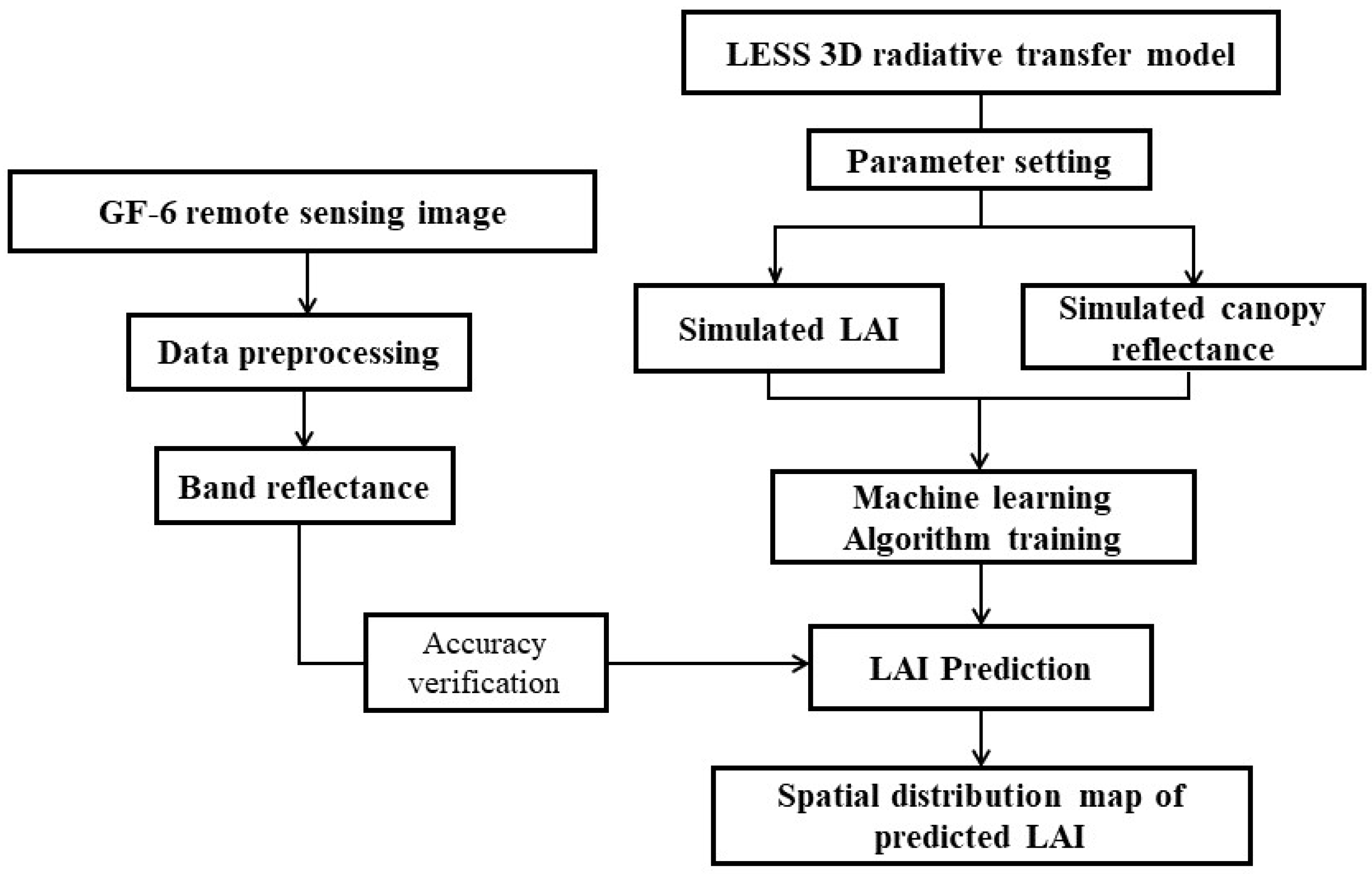
In this study, we primarily utilized the forward ray-tracing principle of the LESS model to calculate the propagation and collision of light rays within the scene. By constructing a 3D realistic forest stand scenario in LESS, we simulated the canopy reflectance of the vegetation within the scene. Additionally, we used the LAI calculator tool to compute the LAI values for each facet unit. The generated data, including both reflectance and LAI values, were subsequently used as the training set for developing the machine learning algorithm. The technical roadmap of the entire study is shown in Figure 2.

2.3. Machine Learning Algorithm

The Random Forest algorithm utilizes ensemble learning principles based on the Bagging concept and decision trees. It employs the bootstrap principle to perform random sampling of both samples and features, generating a host of decision trees. Each tree is trained on a random subset of samples and features from the same dataset [40], and the predictions of multiple decision trees are averaged. Due to sampling with replacement, approximately one-third of the samples are not selected in each iteration, which are called out-of-bag (OOB) samples [41]. The Random Forest algorithm uses the increase in mean squared error (MSE) of the OOB data to estimate the error (OOB error), determines the number of trees, and selects feature variables based on the error rate [42].
E r r o r O O B = 1 n i = 1 n ( y i y i ^ ) 2
In Equation (2), y i ^ indicates the predicted output of out-of-bag (OOB) samples, y i is the actual output, and n represents the total number of OOB samples.
Key parameters in the Random Forest model include mtry, which denotes the number of features used by each tree, and ntree, which represents the total number of trees. These parameters can be adjusted based on the specific situation during model construction [19]. In this study, we found that setting ntree to 600 minimized and stabilized the OOB error. Considering that our model only includes input features from the blue, green, red, and NIR bands, and based on the research by Hultquist et al. [43], who found that the value of mtry has a negligible effect on the accuracy of the Random Forest algorithm, we set mtry to its default value.
The BP Neural Network can be regarded as a special type of multi-layer perceptron, including input, hidden, and output layers. Each layer (potentially having several nodes or neurons) is interconnected but operates independently. The connections between nodes across layers are represented by weights and biases [44]. During propagation, the values of each layer are multiplied by the corresponding weights and added to the biases. The result is then passed through an activation function such as sigmoid (see Equation (3)) and propagated layer by layer to the output layer.
s i g m o i d z = 1 1 + e z ( 0   ,   1 )
If there is a significant discrepancy between the actual output and the desired value, the network computes the sum of squared errors and uses the gradient descent method to perform backpropagation. This process adjusts the network’s weights and biases to bring the error within an acceptable range [45]. When building a BP Neural Network algorithm model, selecting the number of hidden layers and neurons is crucial for optimal performance. The common method for determining the number of hidden layers is through empirical formulas and experiments. Generally, a neural network with one hidden layer is sufficient for many problems and serves as a good starting point. Therefore, in this study, the BP algorithm model is configured with a single hidden layer. To prevent overfitting, we avoided a surplus of neurons in the hidden layer [46]. Based on the experiments, we found that the BP Neural Network model performed most efficiently when the number of nodes was set to 3. Additionally, the learning rate, a hyperparameter that controls step size during gradient descent, significantly affects model performance. A rate that is too high may cause the model to converge to a suboptimal solution quickly, while a rate that is too low can lead to slow convergence. To find the optimal learning rate, we typically use grid search or randomized search methods. In our case, grid search identified 0.1 as the best learning rate. Before training the model, we standardized the data to a range of [−1, 1] to eliminate errors caused by variables.
The XGBoost algorithm is a boosting version of the Gradient Boosting Decision Trees (GBDT) algorithm. Compared to the traditional GBDT algorithm, the XGBoost algorithm has undergone systematic optimization and enhancement in its algorithm structure. It operates on the principle of minimizing the objective function to determine the optimal parameters [47]. The structure of the decision tree relies on calculating the score of each leaf node, applying a regularization function, and establishing the objective function. During the training process, the algorithm fits the residual of the predicted true value from the previous tree, and the final predicted value is obtained by aggregating the predictions of all decision trees.
XGBoost provides support for multiple regularization terms aimed at controlling model complexity, including L1 and L2 regularization [48] to prevent overfitting in the simulation. It also employs column resampling, in addition to traditional row resampling, to further reduce overfitting [49]. There are two parts of the objective function: the loss function and the regularization term, which can be represented by the following equation:
O b j = i = 1 n l ( y i ^ , y i ) + t = 1 k Ω ( f i )
where l is the expression form of the loss function and Ω f i represents the regularization term: Ω f i = γ T + 1 2 λ ω 2 , where T is the number of leaf nodes, ω indicates the modulus of all leaf node vectors, and γ and λ are hyperparameters.
To ensure that the model performs well, it is usually necessary to set hyperparameters, including the maximum depth of the decision tree (max_depth), the learning rate (eta), the minimum leaf node weight, the weak learner type, etc. In this study, we employed five-fold cross-validation to select and optimize parameters for XGBoost, aiming to decide the optimal number of iterations and the best parameters, and then retrain the model. We found that the model achieved the highest accuracy when the number of iterations was set to 11. In the final model parameter settings, the maximum depth of the decision trees (max_depth) was set to 10, the learning rate (eta) was set to 0.2, the minimum weight of the leaf nodes was set to 1, and the booster type was set to the default “gbtree”. Typically, fewer leaf nodes and lower complexity led to higher model accuracy.
The entire modeling process of machine learning algorithms is completed using the R 4.3.3 programming environment. We used the metrics R2 and root mean square error (RMSE) to evaluate the degree of fit and prediction accuracy of the model. The RMSE calculation formula is as follows:
R M S E = i = 1 n ( y i y i ^ ) 2 n  
where y i ^ is the predicted value, y i indicates the measured value, and n represents the data included in the validation set.

2.4. Canopy Reflectance Data Simulation

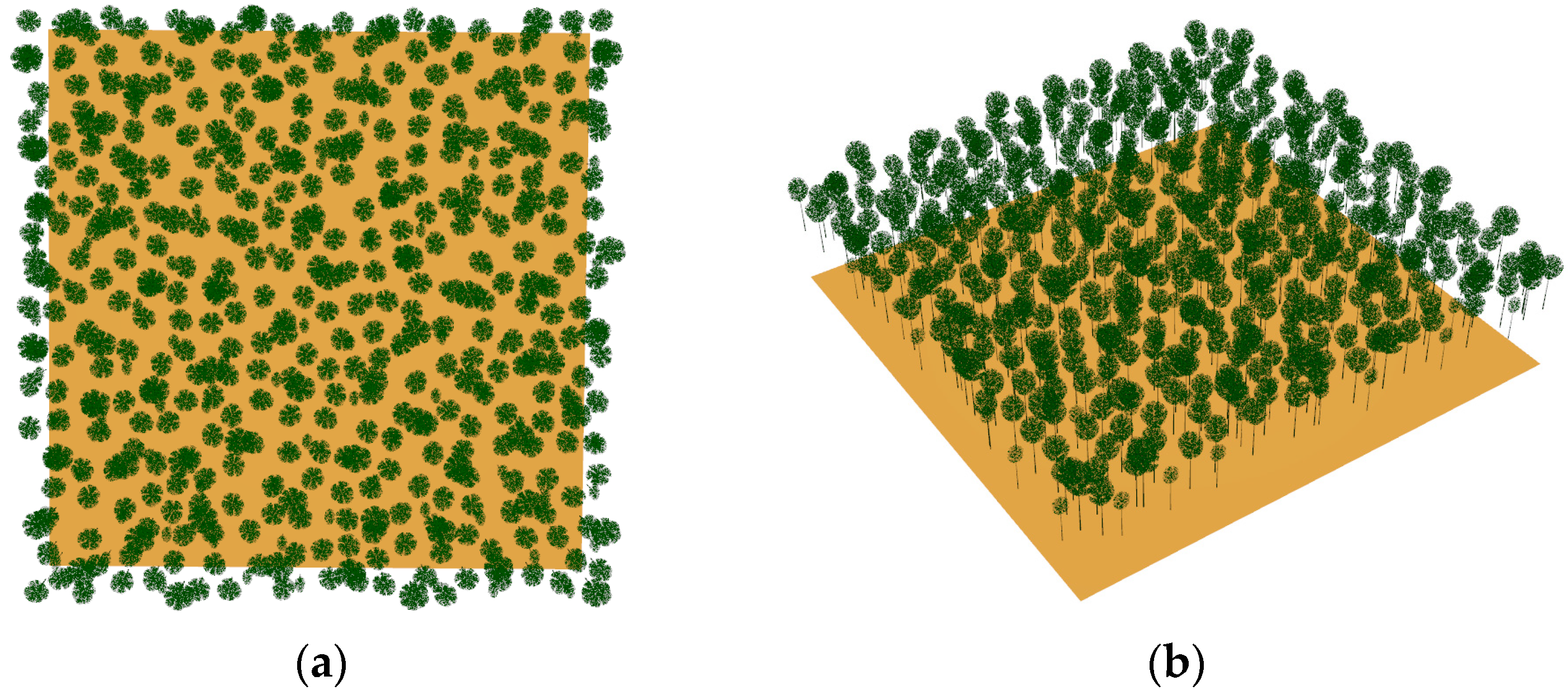
To restore a more realistic 3D forest stand scene in the LESS model, true measured parameters were used, such as crown height, trunk height, branch angle, number of branches, and crown width in the east, west, south, and north when constructing tree structural units. We also attempted to construct multiple tree units with different individual sizes, taking into account the differences in height, spacing, crown width, and other factors among tree species in the real forest stand, and thus established a more realistic 3D structural scene (Figure 3). The spectral characteristics of the tree structure units included those of the trunk, the leaves, and the soil.
The scene size was set to 100 m × 100 m. To ensure that the simulation resolution matched the actual remote sensing imagery and achieved the most realistic simulation results, the width (pixels) and height (pixels) input values were set to 50. This resulted in simulated pixels with a resolution of 2 m, consistent with GF-6 satellite imagery. The solar zenith angle and the azimuth angle were set based on the information provided in the image files, and the proportion of skylight was calculated using the 6s atmospheric transmission model. Leaf spectral information was simulated using the built-in Prospect model. After completing the parameter settings, we ran the LESS simulation to model canopy reflectance. The specific parameter settings are shown in Table 1.

2.5. Multi-Spectral Reflectance Data Conversion

Due to the continuous nature of the simulated spectral reflectance values of the canopy generated by LESS within the range of 400–900 nm with a 1 nm interval, representing an ideal scenario with no errors, and the discrete multi-spectral reflectance values of GF-6 within a certain spectral range, a scale effect emerges between the two sets of values. Therefore, it is necessary to utilize the spectral response function (SRF) of GF-6 satellite imagery to transform the simulated continuous spectral reflectance values into multi-spectral reflectance values that match the actual imagery. This process aims to eliminate the scale effect between the two datasets and restore the spectral information within various wavelength bands relative to the real remote sensing imagery. The integral formula used for this purpose is as follows:
L = λ m i n λ m a x f i ( λ ) L L E S S d λ λ m i n λ m a x f i ( λ ) d λ
where L is the band reflectivity of simulated GF-6, λ m a x and λ m i n are the maximum and minimum wavelength ranges of different bands, respectively, L L E S S denotes the continuous hyperspectral reflectance simulated by the LESS model, and f i ( λ ) is the SRF of the GF-6 sensor.
After integrating the SRF, we transformed the continuous spectral reflectance dataset generated by LESS within the range of 400–900 nm into corresponding multi-spectral reflectance datasets for the blue, green, red, and NIR bands of the GF-6 satellite imagery. These datasets were used as training data for machine learning along with the previously calculated LAI data. In order to overcome data imbalance and enable the model to learn more change patterns and features, thereby reducing the risk of overfitting, we fused 30% of the real data into the training set. We applied stratified sampling to ensure that both simulated and measured data maintained consistency in feature distribution, which involves dividing the data into distinct strata based on key characteristics and then sampling proportionally from each stratum. This approach helps achieve a balanced representation of different data types and improves the model’s ability to generalize. After incorporating part of the real data, the fused data were then divided into a training set (70%) and a testing set (30%) to train three machine learning models.

3. Results

3.1. Random Forest Algorithm Training and Testing

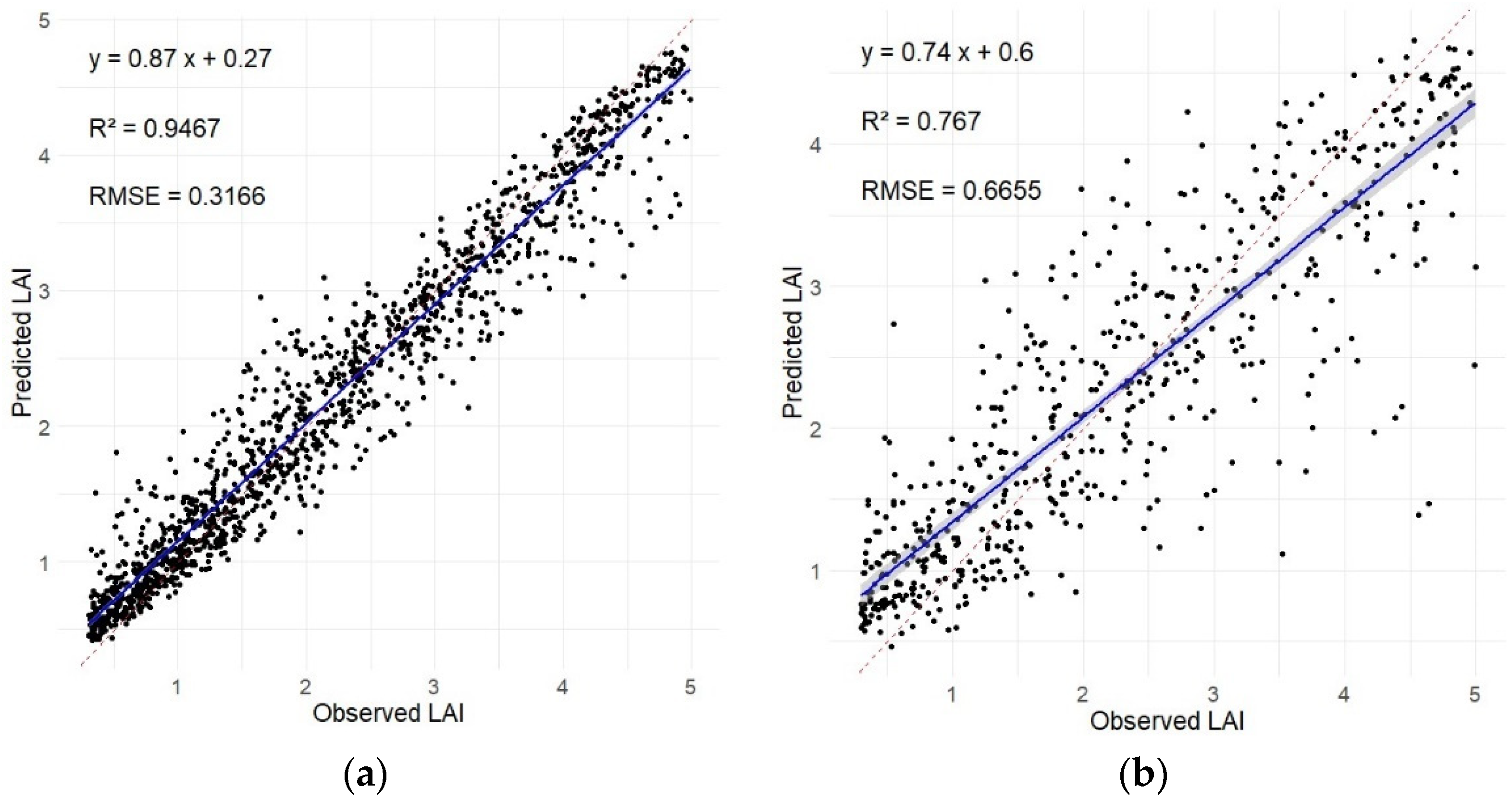
As shown in Figure 4, the Random Forest algorithm achieved outstanding performance on the training dataset, with an R2 of 0.9467 and an RMSE of 0.3166, indicating a precise fit and effectively capturing the features between the data. Subsequently, we tested the model using the testing dataset. The results show that the model also performed well on the testing dataset, with R2 = 0.767 and RMSE = 0.6655, demonstrating high accuracy.

3.2. BP Neural Network Training and Testing

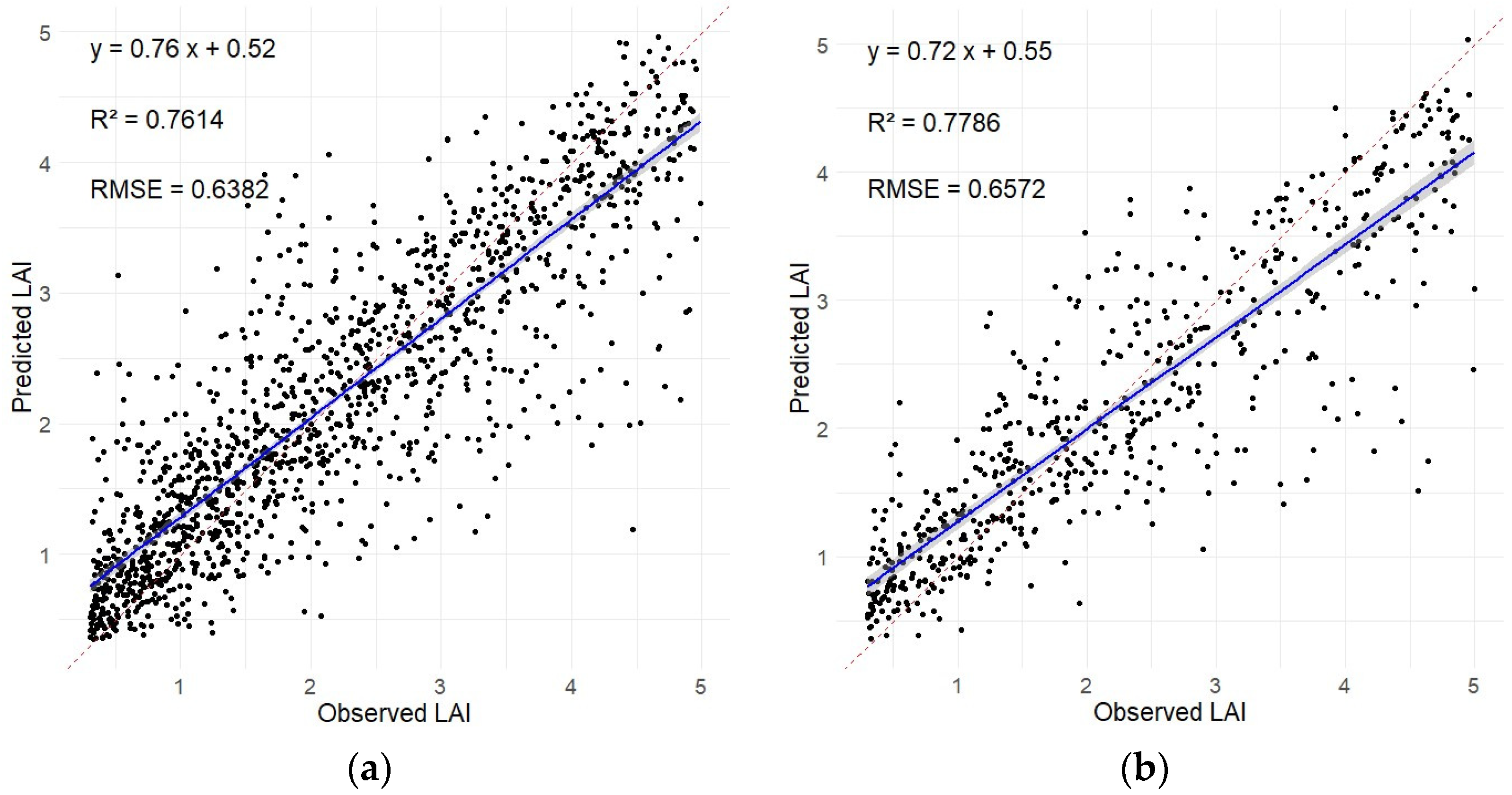
As shown in Figure 5, the performance of the training dataset yielded an R2 of 0.7614 and an RMSE of 0.6382. Although lower than the Random Forest model, the BP Neural Network model still exhibited high accuracy. Moreover, the performance of the testing dataset was very stable, with R2 = 0.7786 and RMSE = 0.6572, even slightly better than the performance of the training dataset, indicating that the model captured and adapted to the features and patterns of the data during testing, showing good stability.

3.3. XGBoost Algorithm Training and Testing

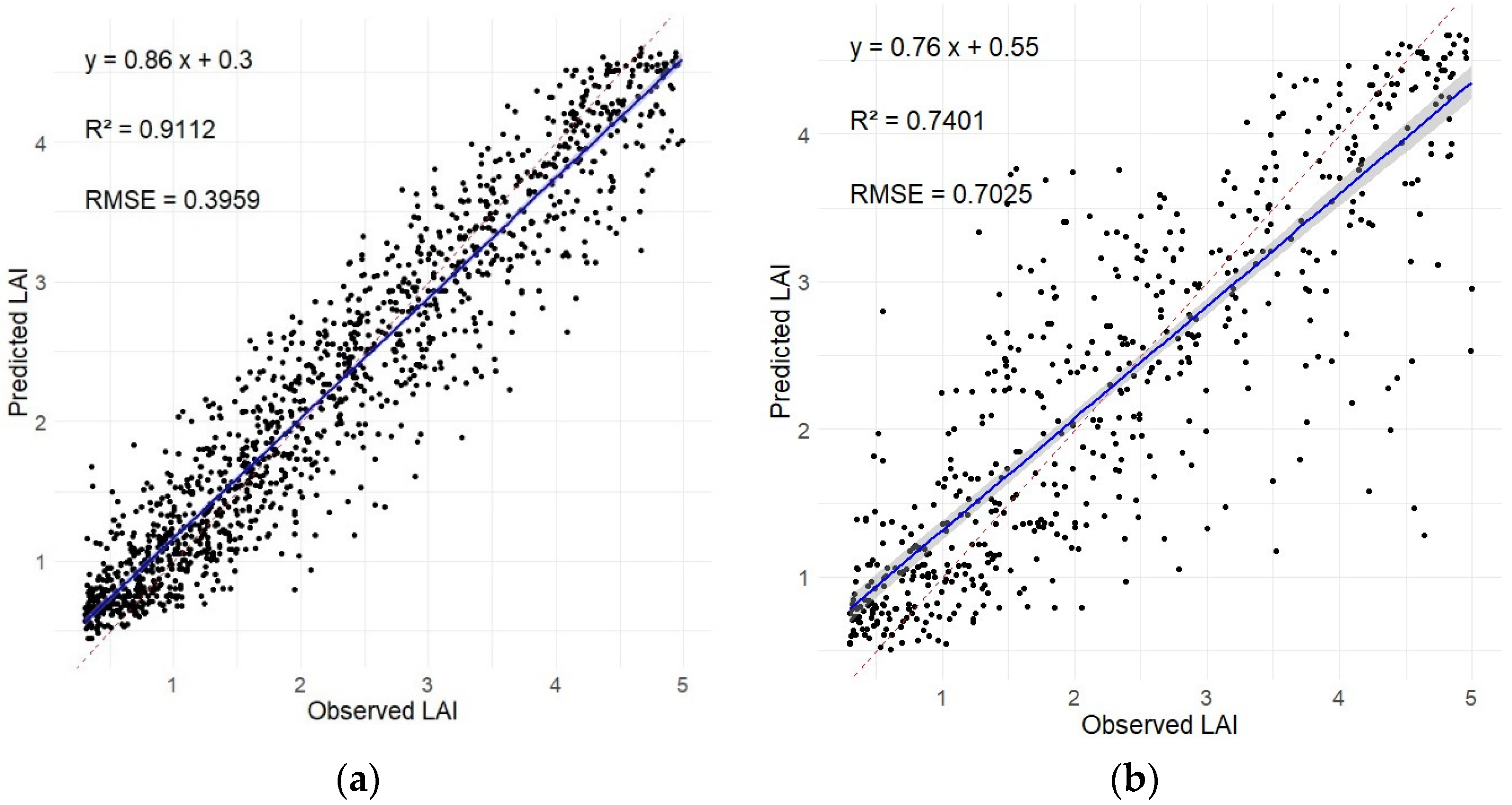
As shown in Figure 6, the model performed well on the training dataset, with an R2 of 0.9112 and an RMSE of 0.3959, approaching the performance of the Random Forest model, showing that the model captured the data effectively. Regarding the performance of the testing dataset, the model still maintained a relatively high precision despite the slight decrease in accuracy, with an R2 of 0.7401 and an RMSE of 0.7025.
Overall, these three machine learning algorithms demonstrated stability and achieved high accuracy during both the training and testing processes. However, the next step should involve further analysis through the validation of the remaining real-world input data.

3.4. Verification Using Measured LAI Values

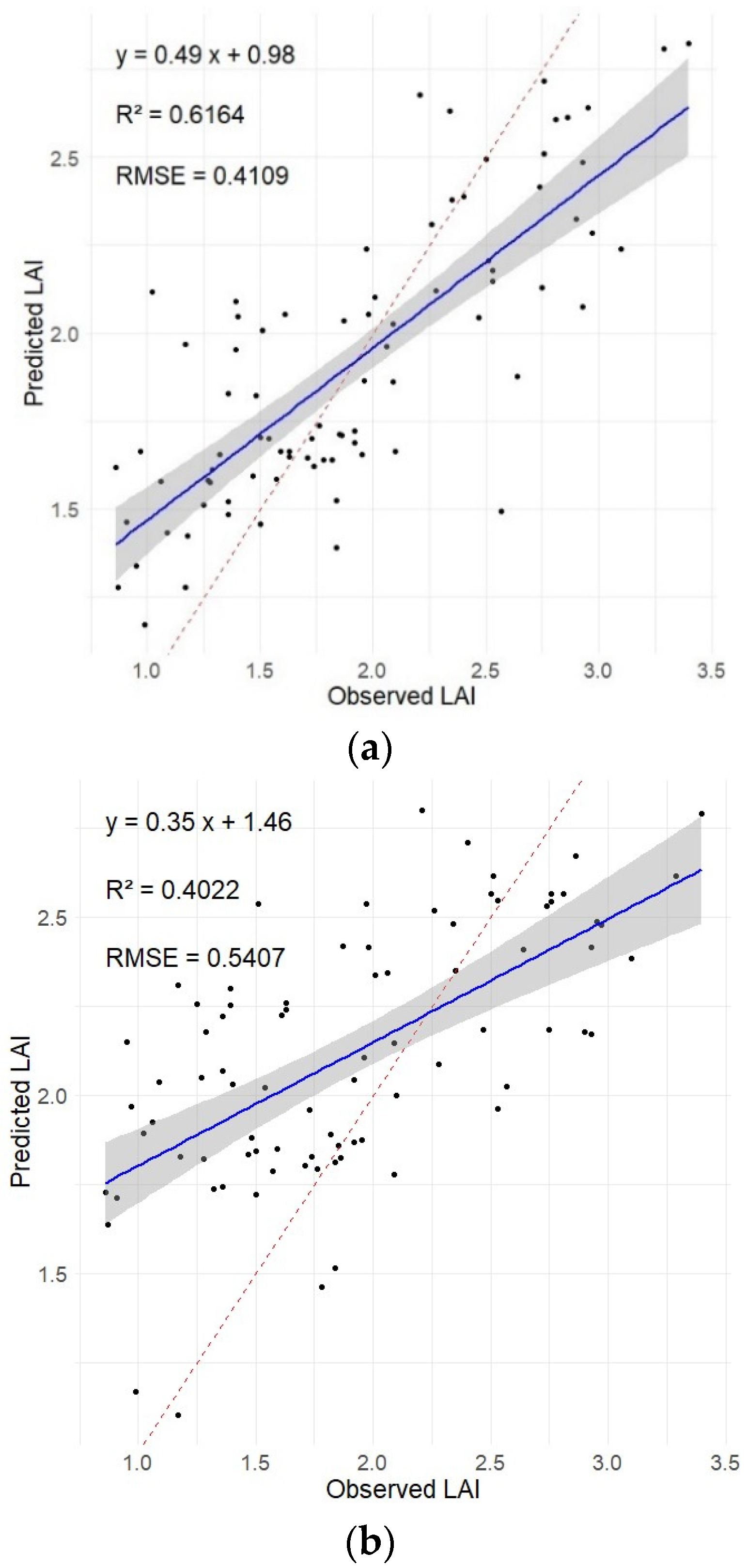
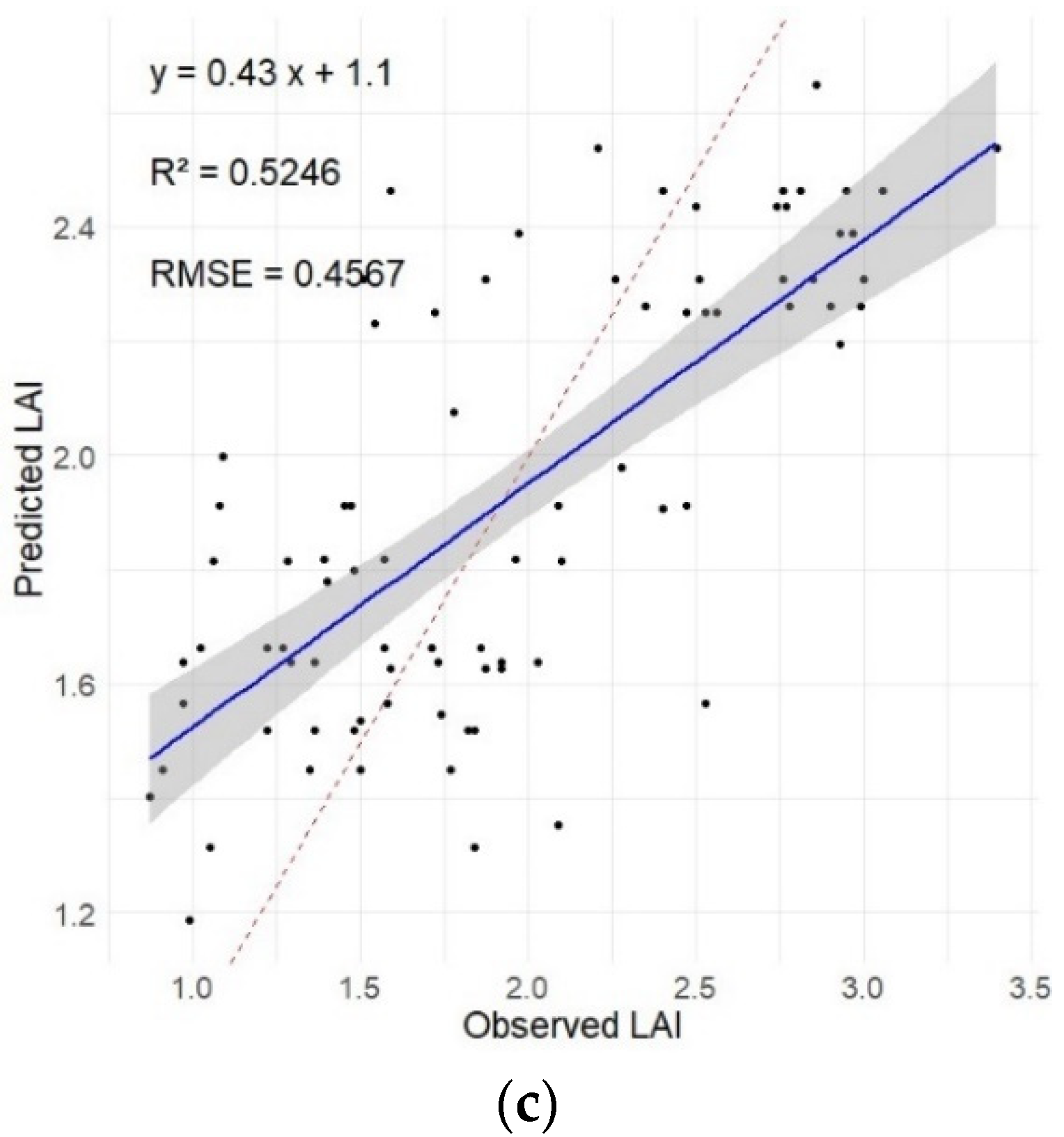
Subsequently, we input the reflectance values of the blue, green, red, and NIR bands extracted from the GF-6 remote sensing images, excluding the fused part, into the trained Random Forest, BP Neural Network, and XGBoost algorithms to predict LAI, and then validated these predictions using the measured LAI values. As shown in Figure 7, the validation results differed somewhat from the model training outcomes. Upon inputting the measured data, the Random Forest algorithm achieved the highest prediction accuracy, with an R2 of 0.6164 and an RMSE of 0.4109, outperforming the other algorithms. The XGBoost algorithm also demonstrated high prediction accuracy, with R2 = 0.5246 and RMSE = 0.4567. Conversely, the BP Neural Network algorithm yielded the lowest prediction accuracy, with an R² of only 0.4022 and an RMSE of 0.5407, demonstrating poor performance.
In this experiment, although the BP Neural Network showed stable performance during training and testing, it struggled to adapt to the input of unfamiliar measured data, indicating that the model did not fully converge. This could be due to the limitations of the BP algorithm’s use of the gradient descent method to reduce errors. Despite the presence of backpropagation, the model could not cover the entire parameter space and often only found local optimal solutions. Additionally, determining the optimal number of hidden neurons using heuristic methods is challenging.
In contrast, the Random Forest and XGBoost algorithms performed excellently. Although their validation accuracy on the test set was not as high as that of the BP Neural Network algorithm, they handled unfamiliar data more effectively, especially when dealing with nonlinear data. This finding highlights the advantages of ensemble learning, demonstrating that the aggregated predictions of multiple decision trees can effectively address the limitations of data training, significantly improve model prediction accuracy, and effectively handle overfitting and noise data [50]. However, the R2 value of the Random Forest on the validation set, which performed the best, is lower than 0.65, indicating the possibility of error sources in practical applications. According to previous research, the complexity of ground features, including terrain undulations and variability in ground reflectance, can significantly affect model performance [51,52]. These factors can lead to high spatial heterogeneity in the true values of the Leaf Area Index, and random forest models may find it difficult to capture these complex spatial relationships [53]. In addition, the measurement accuracy and collection conditions of ground data also affect the performance of the model [54,55]. Minor changes in ground features may be overlooked in measurements, but they significantly affect the results in model predictions. The existence of complex features poses challenges for models in practical applications, and future research needs to further consider the potential impact of these factors on model performance. Overall, the Random Forest algorithm, with its high model stability and robustness, is well-suited for LAI inversion tasks.

3.5. LAI Inversion Spatial Distribution Maps

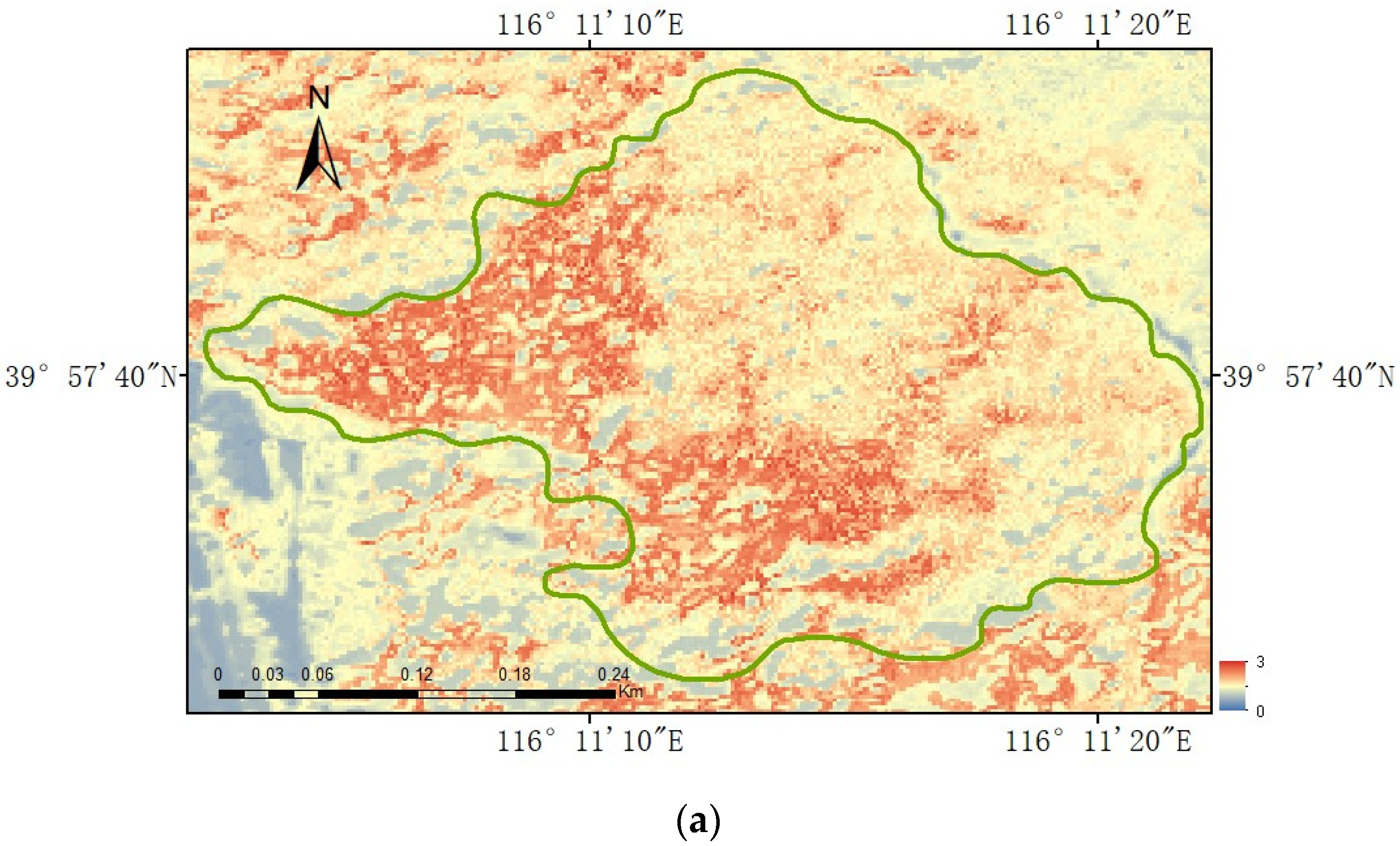
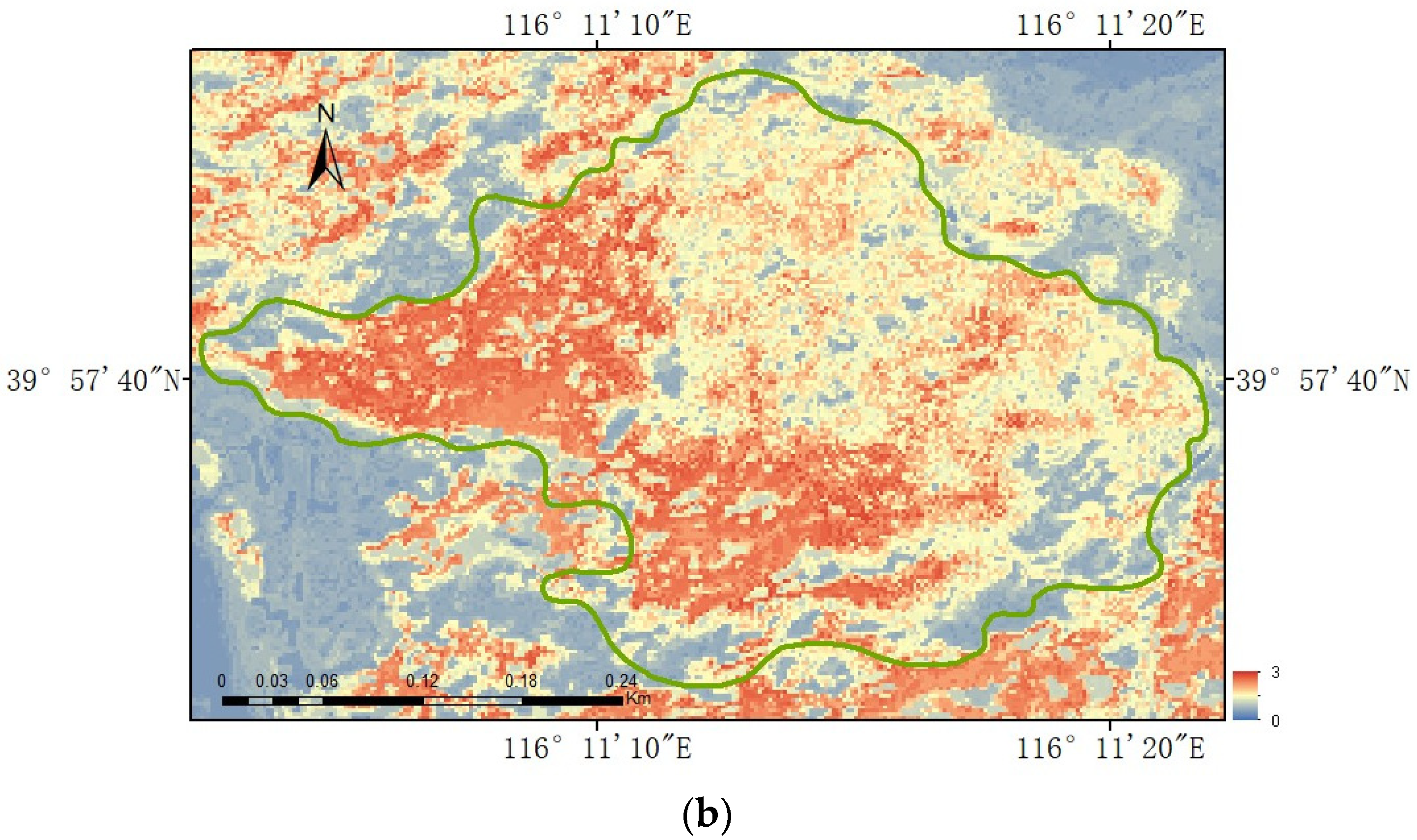
Based on the aforementioned model validation results, we selected the Random Forest and XGBoost algorithms to perform LAI inversion and generated the corresponding LAI spatial distribution maps (Figure 8). We unified the range of its values in the layer display to [0, 3]. The LAI values predicted by the Random Forest inversion ranged from 0.4630 to 2.8349, while the LAI values predicted by XGBoost ranged from 0.4161 to 2.6496. Both tend to slightly underestimate the true value. In comparison, the inversion result of Random Forest is closer to the true value.
The inversion results further demonstrate that the Random Forest algorithm can effectively overcome the influence of noise and has a more accurate performance, with its predicted results being basically consistent with the actual situation. Therefore, we believe that the Random Forest algorithm is the most suitable choice for LAI inversion in this study area, and can also be one of the preferred machine learning algorithms in other inversion studies.

4. Discussion

In the description of ecosystem structure, the Leaf Area Index (LAI) is a crucial parameter. In recent years, research on LAI inversion has increasingly deepened, and its combination with 3D Radiative Transfer Models (RTM) has been widely applied. The LESS model has gained wide acceptance in the field of remote sensing with its user-friendly interface and rich functionality. The accuracy of LESS has been confirmed through ground observations and benchmark models [56]. Most of the default parameter settings in LESS are based on actual measurements and are suitable for most scenarios. For more details, please refer to https://lessrt.org/, accessed on 21 November 2023. Compared to previous models, LESS has significant advantages in simulating canopy structure and computational accuracy. For instance, the study by Ouyang et al. [57] pointed out that the widely used PROSAIL model represents the canopy as a horizontally uniform turbid medium, ignoring the fine structure within the canopy. Lu [58] also found that although it is suitable for multi-leaf and uniform canopies, it performs poorly in dense forests or mixed ecosystems. Additionally, the study by Landier [59] showed that while most current 3D radiative transfer models, such as DART, offer significant advantages in accuracy, they still exhibit relatively high computational complexity and resource consumption when dealing with complex structural scenes, requiring greater computational costs and higher data resolution. In contrast, the LESS model used in this study can better capture the scattering and absorption processes of light by modeling the detailed three-dimensional structure of the canopy [36], thereby significantly improving the accuracy of LAI estimation. The triangular patch structure of the LESS model greatly simplifies memory usage and improves computational efficiency.
In this study, we used LESS to recreate a realistic forest stand scene. The leaf reflectance and transmittance spectral information were calculated using the built-in Prospect model, and the spectral characteristics of the soil were simulated using the Gsv model. Vegetation canopy reflectance and LAI in the scene were then simulated to generate the training dataset for the machine learning algorithms. We also attempted to build Random Forest, BP Neural Network, and XGBoost models. Although the BP Neural Network performed well on the training and test sets, its accuracy on measured data was poor, with an R2 of only 0.4022 and an RMSE of 0.5407. We analyzed the potential reasons for this. When using a fixed learning rate, the BP Neural Network algorithm converges slowly, which can cause oscillations and fluctuations as it approaches the optimal solution. Additionally, because the activation function’s range is usually limited (typically between 0 and 1), inconsistencies can occur in the change patterns across layers. This leads to discrepancies between predictions and training data or limited extrapolation capabilities [60]. Multiple studies have indicated that BP Neural Networks highly depend on training data and are relatively inaccurate in predicting unseen data [61,62], similar to the findings of this study.
In contrast, the Random Forest and XGBoost algorithms demonstrated satisfactory accuracy. The XGBoost model achieved an R2 of 0.5246 and an RMSE of 0.4567, while the Random Forest model achieved an R2 of 0.6164 and an RMSE of 0.4109, demonstrating an even more accurate performance. Therefore, we opted for the Random Forest and XGBoost algorithms to generate the LAI spatial distribution maps. The LAI inversion values predicted by the Random Forest algorithm were closer to the true LAI values, further confirming its superiority. With its robust capacity to handle large-scale and complex data processing tasks, it is highly suitable for LAI inversion in the study area.
Moreover, the LESS model is particularly well suited for forest canopy inversion due to its straightforward parameter settings and integrated coupling models. Compared with traditional radiative transfer models, which may require complex parameter adjustments and struggle with the intricate structure of forest canopies, LESS simplifies the process by providing built-in models that are specifically tailored for forest environments. This ease of use and inherent model integration offer a significant advantage over previous models, making LESS a more effective and user-friendly solution for accurately modeling forest canopies.

5. Conclusions

In conclusion, this study concentrates on the application of the LESS 3D RTM in conjunction with machine learning algorithms and GF-6 multi-spectral images to achieve the inversion of the forest stand Leaf Area Index (LAI) in the study area of Xishan Experimental Forest Farm in Beijing, China. We introduced different machine learning forces by establishing Random Forest, BP Neural Network, and XGBoost models. Random Forest was finally used to achieve high-precision LAI inversion and prediction, fully demonstrating its efficiency and stability and thus providing a powerful tool for forest LAI inversion.
It is worth noting that although this study has achieved significant results and shows potential for further investigation, it still presents certain limitations. The study area is relatively limited, and combined with seasonal changes and climatic elements as well as other environmental factors, multi-indicator comprehensive research should be conducted to comprehensively understand the dynamic changes of ecosystems. In LAI inversion studies, different regions typically have varying topographical conditions, which can lead to errors in LAI inversion. Generally, the error in retrieved LAI values increases with the slope of the terrain [63]. In practical scenarios, land cover conditions contribute to pixel heterogeneity within the study area, while atmospheric differences between pixels can affect radiative transfer due to terrain features, further influencing LAI accuracy [64,65]. Moreover, variations in precipitation and temperature influence vegetation growth rates and canopy structure [66,67]. Changes in cloud cover and lighting conditions can also affect the quality of remote sensing data [68], thus impacting LAI inversion results. In future studies, we should consider integrating multi-source remote sensing data, such as combining optical remote sensing with LiDAR data, to enhance estimation accuracy. It is important to develop more sophisticated models and algorithms, optimize parameters to fit specific regional and climatic conditions, and design inversion methods tailored to various topographic types. Additionally, exploring the stability and temporal consistency of LAI inversion models across different time series is a key research topic with significant implications for enhancing the reliability and accuracy of LAI estimates. Overall, this study provides crucial theoretical and methodological support for the research and practical applications of LAI inversion in forest stands, offering valuable references for other related studies.

Author Contributions

Conceptualization, F.F.; Formal analysis, Z.Z.; Writing—original draft, Y.J.; Writing—review & editing, R.L.; Supervision, X.Z. and C.X.; Project administration, H.H. and M.Z. All authors have read and agreed to the published version of the manuscript.

Funding

This research was supported by “National Natural Science Foundation of China (32271832)” and “Key Project of National Key Research and Development Plan (2023YFF1304004-06)”.

Data Availability Statement

The datasets used in this research can be obtained with the permission of the corresponding and first author if there is a legitimate need.

Conflicts of Interest

The authors declare no conflict of interest.

References

  1. Fang, H.; Baret, F.; Plummer, S.; Schaepman-Strub, G. An Overview of Global Leaf Area Index (LAI): Methods, Products, Validation, and Applications. Rev. Geophys. 2019, 57, 739–799. [Google Scholar] [CrossRef]
  2. Lu, X.; Wang, X.; Yang, Z. Leaf area index estimation from the time-series SAR data using the AIEM-MWCM model. Int. J. Digit. Earth 2023, 16, 4385–4403. [Google Scholar] [CrossRef]
  3. Mastro, P.; Peppo, M.D.; Crema, A.; Boschetti, M.; Pepe, A. Statistical characterization and exploitation of Synthetic Aperture radar vegetation indexes for the generation of Leaf area Index time series. Int. J. Appl. Earth Obs. Geoinf. 2023, 124, 103498. [Google Scholar] [CrossRef]
  4. Weiss, M.; Baret, F.; Smith, G.J.; Jonckheere, I.; Coppin, P. Review of methods for in situ leaf area index (LAI) determination. Agric. For. Meteorol. 2004, 121, 37–53. [Google Scholar] [CrossRef]
  5. Chen, J.M.; Black, T.A. Defining leaf area index for non-flat leaves. Plant Cell Environ. 1992, 15, 421–429. [Google Scholar] [CrossRef]
  6. Wang, X.; Lu, X.; Yang, Z. A MWCMLAI-Net method for LAI inversion in maize and rice using GF-3 and Lutan radar data. Int. J. Digit. Earth 2024, 17, 2341128. [Google Scholar] [CrossRef]
  7. Parker, G.G. Tamm review: Leaf Area Index (LAI) is both a determinant and a consequence of important processes in vegetation canopies. For. Ecol. Manag. 2020, 477, 118496. [Google Scholar] [CrossRef]
  8. Kalisperakis, I.; Stentoumis, C.; Grammatikopoulos, L.; Karantzalos, K. Leaf Area Index Estimation in Vineyards from Uav Hyperspectral Data, 2D Image Mosaics and 3D Canopy Surface Models. Int. Arch. Photogramm. Remote Sens. Spat. Inf. Sci. 2015, XL-1/W4, 299–303. [Google Scholar] [CrossRef]
  9. Cohen, W.B.; Maiersperger, T.K.; Gower, S.T.; Turner, D.P. An improved strategy for regression of biophysical variables and Landsat ETM+ data. Remote Sens. Environ. 2003, 84, 561–571. [Google Scholar] [CrossRef]
  10. Luo, S.-Z.; Wang, C.; Zhang, G.-B.; Xi, X.-H.; Li, G.-C. Forest Leaf Area Index (LAI) Estimation Using Airborne Discrete-Return Lidar Data. Chin. J. Geophys. 2013, 56, 233–242. [Google Scholar] [CrossRef]
  11. Ollinger, S.V. Sources of variability in canopy reflectance and the convergent properties of plants. New Phytol. 2011, 189, 375–394. [Google Scholar] [CrossRef] [PubMed]
  12. Nadkarni, N.M.; Parker, G.G.; Lowman, M.D. Forest canopy studies as an emerging field of science. Ann. For. Sci. 2011, 68, 217. [Google Scholar] [CrossRef]
  13. Breda, N.J.J. Ground-based measurements of leaf area index: A review of methods, instruments and current controversies. J. Exp. Bot. 2003, 54, 2403–2417. [Google Scholar] [CrossRef]
  14. Song, B.; Liu, L.; Zhao, J.; Chen, X.; Zhang, H.; Gao, Y.; Zhang, X. Validation of Four Coarse-Resolution Leaf Area Index Products Over Croplands in China Using Field Measurements. IEEE J. Sel. Top. Appl. Earth Obs. Remote Sens. 2021, 14, 9372–9382. [Google Scholar] [CrossRef]
  15. Wang, Y.; Fang, H. Estimation of LAI with the LiDAR Technology: A Review. Remote Sens. 2020, 12, 3457. [Google Scholar] [CrossRef]
  16. Eklundh, L.; Harrie, L.; Kuusk, A. Investigating relationships between Landsat ETM+ sensor data and leaf area index in a boreal conifer forest. Remote Sens. Environ. 2001, 78, 239–251. [Google Scholar] [CrossRef]
  17. Li, Z.; Xin, X.; Tang, H.; Yang, F.; Chen, B.; Zhang, B. Estimating grassland LAI using the Random Forests approach and Landsat imagery in the meadow steppe of Hulunber, China. J. Integr. Agric. 2017, 16, 286–297. [Google Scholar] [CrossRef]
  18. Verrelst, J.; Schaepman, M.E.; Malenovský, Z.; Clevers, J.G.P.W. Effects of woody elements on simulated canopy reflectance: Implications for forest chlorophyll content retrieval. Remote Sens. Environ. 2010, 114, 647–656. [Google Scholar] [CrossRef]
  19. Srinet, R.; Nandy, S.; Patel, N.R. Estimating leaf area index and light extinction coefficient using Random Forest regression algorithm in a tropical moist deciduous forest, India. Ecol. Inform. 2019, 52, 94–102. [Google Scholar] [CrossRef]
  20. Houborg, R.; Boegh, E. Mapping leaf chlorophyll and leaf area index using inverse and forward canopy reflectance modeling and SPOT reflectance data. Remote Sens. Environ. 2008, 112, 186–202. [Google Scholar] [CrossRef]
  21. Houborg, R.; Soegaard, H.; Boegh, E. Combining vegetation index and model inversion methods for the extraction of key vegetation biophysical parameters using Terra and Aqua MODIS reflectance data. Remote Sens. Environ. 2007, 106, 39–58. [Google Scholar] [CrossRef]
  22. Peng, S.; Wang, Z.; Lu, X.; Liu, X. Hybrid inversion of radiative transfer models based on topographically corrected Landsat surface reflectance improves leaf area index and aboveground biomass retrievals of grassland on the hilly Loess Plateau. Int. J. Digit. Earth 2024, 17, 2316840. [Google Scholar] [CrossRef]
  23. Schlerf, M.; Atzberger, C. Inversion of a forest reflectance model to estimate structural canopy variables from hyperspectral remote sensing data. Remote Sens. Environ. 2006, 100, 281–294. [Google Scholar] [CrossRef]
  24. Darvishzadeh, R.; Wang, T.; Skidmore, A.; Vrieling, A.; O’Connor, B.; Gara, T.; Ens, B.; Paganini, M. Analysis of Sentinel-2 and RapidEye for Retrieval of Leaf Area Index in a Saltmarsh Using a Radiative Transfer Model. Remote Sens. 2019, 11, 671. [Google Scholar] [CrossRef]
  25. Schneider, F.D.; Leiterer, R.; Morsdorf, F.; Gastellu-Etchegorry, J.-P.; Lauret, N.; Pfeifer, N.; Schaepman, M.E. Simulating imaging spectrometer data: 3D forest modeling based on LiDAR and in situ data. Remote Sens. Environ. 2014, 152, 235–250. [Google Scholar] [CrossRef]
  26. Wang, Y.; Lauret, N.; Gastellu-Etchegorry, J.-P. DART radiative transfer modelling for sloping landscapes. Remote Sens. Environ. 2020, 247, 111902. [Google Scholar] [CrossRef]
  27. North, P.R.J. Three-dimensional forest light interaction model using a Monte Carlo method. IEEE Trans. Geosci. Remote Sens. 1996, 34, 946–956. [Google Scholar] [CrossRef]
  28. Govaerts, Y.M.; Verstraete, M.M. Raytran: A Monte Carlo ray-tracing model to compute light scattering in three-dimensional heterogeneous media. IEEE Trans. Geosci. Remote Sens. 1998, 36, 493–505. [Google Scholar] [CrossRef]
  29. Qin, W.; Gerstl, S.A.W. 3-D Scene Modeling of Semidesert Vegetation Cover and its Radiation Regime. Remote Sens. Environ. 2000, 74, 145–162. [Google Scholar] [CrossRef]
  30. Huang, H.; Qin, W.; Liu, Q. RAPID: A Radiosity Applicable to Porous IndiviDual Objects for directional reflectance over complex vegetated scenes. Remote Sens. Environ. 2013, 132, 221–237. [Google Scholar] [CrossRef]
  31. Dai, Z.; Ding, Y.; Xu, C.; Chen, Y.; Liu, L. Evaluation of the impact of crop residue on fractional vegetation cover estimation by vegetation indices over conservation tillage cropland: A simulation study. Int. J. Remote Sens. 2022, 43, 6463–6482. [Google Scholar] [CrossRef]
  32. Qi, J.; Xie, D.; Guo, D.; Yan, G. A Large-Scale Emulation System for Realistic Three-Dimensional (3-D) Forest Simulation. IEEE J. Sel. Top. Appl. Earth Obs. Remote Sens. 2017, 10, 4834–4843. [Google Scholar] [CrossRef]
  33. Qi, J.; Xie, D. LESS: A Model for Radiative Transfer Simulation in Heterogeneous 3D Vegetation Canopies. In AGU Fall Meeting Abstracts; Jianbo Qi: Beijing, China, 2021; Volume 2021, p. B52D-04. [Google Scholar]
  34. Wu, Q.; Yang, S.; Jiang, J. Impacts of clumping effect on canopy reflectance using 3D radiative transfer modeling. Front. For. Glob. Chang. 2023, 6, 1106773. [Google Scholar] [CrossRef]
  35. Cheng, J.; Yang, H.; Qi, J.; Sun, Z.; Han, S.; Feng, H.; Jiang, J.; Xu, W.; Li, Z.; Yang, G.; et al. Estimating canopy-scale chlorophyll content in apple orchards using a 3D radiative transfer model and UAV multispectral imagery. Comput. Electron. Agric. 2022, 202, 107401. [Google Scholar] [CrossRef]
  36. Qi, J.; Jiang, J.; Zhou, K.; Xie, D.; Huang, H. Fast and Accurate Simulation of Canopy Reflectance under Wavelength-Dependent Optical Properties Using a Semi-Empirical 3D Radiative Transfer Model. J. Remote Sens. 2023, 3, 0017. [Google Scholar] [CrossRef]
  37. Qi, J.; Xie, D.; Jiang, J.; Huang, H. 3D radiative transfer modeling of structurally complex forest canopies through a lightweight boundary-based description of leaf clusters. Remote Sens. Environ. 2022, 283, 113301. [Google Scholar] [CrossRef]
  38. Zhou, K.; Xie, D.; Qi, J.; Zhang, Z.; Bo, X.; Yan, G.; Mu, X. Explicitly Reconstructing RAMI-V Scenes for Accurate 3-Dimensional Radiative Transfer Simulation Using the LESS Model. J. Remote Sens. 2023, 3, 0033. [Google Scholar] [CrossRef]
  39. Qi, J.; Xie, D.; Yin, T.; Yan, G.; Gastellu-Etchegorry, J.-P.; Li, L.; Zhang, W.; Mu, X.; Norford, L.K. LESS: LargE-Scale remote sensing data and image simulation framework over heterogeneous 3D scenes. Remote Sens. Environ. 2019, 221, 695–706. [Google Scholar] [CrossRef]
  40. Houborg, R.; McCabe, M.F. A hybrid training approach for leaf area index estimation via Cubist and random forests machine-learning. ISPRS J. Photogramm. Remote Sens. 2018, 135, 173–188. [Google Scholar] [CrossRef]
  41. Belgiu, M.; Drăguţ, L. Random forest in remote sensing: A review of applications and future directions. ISPRS J. Photogramm. Remote Sens. 2016, 114, 24–31. [Google Scholar] [CrossRef]
  42. Prasad, A.M.; Iverson, L.R.; Liaw, A. Newer Classification and Regression Tree Techniques: Bagging and Random Forests for Ecological Prediction. Ecosystems 2006, 9, 181–199. [Google Scholar] [CrossRef]
  43. Hultquist, C.; Chen, G.; Zhao, K. A comparison of Gaussian process regression, random forests and support vector regression for burn severity assessment in diseased forests. Remote Sens. Lett. 2014, 5, 723–732. [Google Scholar] [CrossRef]
  44. Ji, C.; Ding, H. Optimizing Back-Propagation Neural Network to Retrieve Sea Surface Temperature Based on Improved Sparrow Search Algorithm. Remote Sens. 2023, 15, 5722. [Google Scholar] [CrossRef]
  45. Yu, W.; Xu, X.; Jin, S.; Ma, Y.; Liu, B.; Gong, W. BP Neural Network Retrieval for Remote Sensing Atmospheric Profile of Ground-Based Microwave Radiometer. IEEE Geosci. Remote Sens. Lett. 2022, 19, 4502105. [Google Scholar] [CrossRef]
  46. Ma, J.; Wang, L.; Chen, P. Comparing Different Methods for Wheat LAI Inversion Based on Hyperspectral Data. Agriculture 2022, 12, 1353. [Google Scholar] [CrossRef]
  47. Budholiya, K.; Shrivastava, S.K.; Sharma, V. An optimized XGBoost based diagnostic system for effective prediction of heart disease. J. King Saud Univ.-Comput. Inf. Sci. 2022, 34, 4514–4523. [Google Scholar] [CrossRef]
  48. Militino, A.F.; Goyena, H.; Pérez-Goya, U.; Ugarte, M.D. Logistic regression versus XGBoost for detecting burned areas using satellite images. Environ. Ecol. Stat. 2024, 31, 57–77. [Google Scholar] [CrossRef]
  49. Florea, A.-C.; Andonie, R. Weighted Random Search for Hyperparameter Optimization. Int. J. Comput. Commun. Control 2019, 14, 154–169. [Google Scholar] [CrossRef]
  50. Heung, B.; Bulmer, C.E.; Schmidt, M.G. Predictive soil parent material mapping at a regional-scale: A Random Forest approach. Geoderma 2014, 214–215, 141–154. [Google Scholar] [CrossRef]
  51. Xie, X.; Tian, J.; Wu, C.; Li, A.; Jin, H.; Bian, J.; Zhang, Z.; Nan, X.; Jin, Y. Long-term topographic effect on remotely sensed vegetation index-based gross primary productivity (GPP) estimation at the watershed scale. Int. J. Appl. Earth Obs. Geoinf. 2022, 108, 102755. [Google Scholar] [CrossRef]
  52. Ma, Y.; He, T.; McVicar, T.R.; Liang, S.; Liu, T.; Peng, W.; Song, D.-X.; Tian, F. Quantifying how topography impacts vegetation indices at various spatial and temporal scales. Remote Sens. Environ. 2024, 312, 114311. [Google Scholar] [CrossRef]
  53. Wang, Y.; Wu, K.; Qin, J.; Wang, C.; Zhang, H. Examining Spatial Heterogeneity Effects of Landscape and Environment on the Residential Location Choice of the Highly Educated Population in Guangzhou, China. Sustainability 2020, 12, 3869. [Google Scholar] [CrossRef]
  54. Ekström, T.; Burke, S.; Wiktorsson, M.; Hassanie, S.; Harderup, L.-E.; Arfvidsson, J. Evaluating the impact of data quality on the accuracy of the predicted energy performance for a fixed building design using probabilistic energy performance simulations and uncertainty analysis. Energy Build. 2021, 249, 111205. [Google Scholar] [CrossRef]
  55. Yamaguchi, T.; Sasano, K.; Katsura, K. Improving efficiency of ground-truth data collection for UAV-based rice growth estimation models: Investigating the effect of sampling size on model accuracy. Plant Prod. Sci. 2024, 27, 1–13. [Google Scholar] [CrossRef]
  56. Gao, S.; Yan, K.; Liu, J.; Pu, J.; Zou, D.; Qi, J.; Mu, X.; Yan, G. Assessment of remote-sensed vegetation indices for estimating forest chlorophyll concentration. Ecol. Indic. 2024, 162, 112001. [Google Scholar] [CrossRef]
  57. Ouyang, L.; Qi, J.; Wang, Q.; Jia, K.; Cao, B.; Zhao, W. MART3D: A Multilayer Heterogeneous 3D Radiative Transfer Framework for Characterizing Forest Disturbances. Forests 2024, 15, 824. [Google Scholar] [CrossRef]
  58. Lu, B.; Proctor, C.; He, Y. Investigating different versions of PROSPECT and PROSAIL for estimating spectral and biophysical properties of photosynthetic and non-photosynthetic vegetation in mixed grasslands. GIScience Remote Sens. 2021, 58, 354–371. [Google Scholar] [CrossRef]
  59. Landier, L.; Gastellu-Etchegorry, J.P.; Al Bitar, A.; Chavanon, E.; Lauret, N.; Feigenwinter, C.; Mitraka, Z.; Chrysoulakis, N. Calibration of urban canopies albedo and 3D shortwave radiative budget using remote-sensing data and the DART model. Eur. J. Remote Sens. 2018, 51, 739–753. [Google Scholar] [CrossRef]
  60. Jiquan, W.; Lichun, Q.; Guilian, L.; Fulin, W. The Problems and Its Analysis of BP Neural Network. In Proceedings of the 2010 International Conference on Intelligent System Design and Engineering Application, Changsha, China, 13–14 October 2010; IEEE: Changsha, China, 2010; pp. 701–704. [Google Scholar]
  61. Li, H.; Khazanovich, L. Multi-gene genetic programming extension of AASHTO M-E for design of low-volume concrete pavements. J. Road Eng. 2022, 2, 252–266. [Google Scholar] [CrossRef]
  62. Kronberger, G.; De Franca, F.O.; Burlacu, B.; Haider, C.; Kommenda, M. Shape-Constrained Symbolic Regression—Improving Extrapolation with Prior Knowledge. Evol. Comput. 2022, 30, 75–98. [Google Scholar] [CrossRef]
  63. Mousivand, A.; Verhoef, W.; Menenti, M.; Gorte, B. Modeling Top of Atmosphere Radiance over Heterogeneous Non-Lambertian Rugged Terrain. Remote Sens. 2015, 7, 8019–8044. [Google Scholar] [CrossRef]
  64. Zheng, Y.; Xiao, Z.; Shi, H.; Song, J. Exploring the Effects of Topography on Leaf Area Index Retrieved from Remote Sensing Data at Various Spatial Scales over Rugged Terrains. Remote Sens. 2024, 16, 1404. [Google Scholar] [CrossRef]
  65. Shi, H.; Xiao, Z.; Wen, J.; Wu, S. An Optical–Thermal Surface–Atmosphere Radiative Transfer Model Coupling Framework With Topographic Effects. IEEE Trans. Geosci. Remote Sens. 2022, 60, 4400312. [Google Scholar] [CrossRef]
  66. Zhang, Y.; Hou, J.; Han, W.; Dou, P.; Huang, C. Spatio-temporal analysis of LAI using multisource remote sensing data for source region of Yellow River Basin. Front. Environ. Sci. 2024, 12, 1320881. [Google Scholar] [CrossRef]
  67. Lafortezza, R.; Giannico, V. Combining high-resolution images and LiDAR data to model ecosystem services perception in compact urban systems. Ecol. Indic. 2019, 96, 87–98. [Google Scholar] [CrossRef]
  68. Gawlikowski, J.; Ebel, P.; Schmitt, M.; Zhu, X.X. Explaining the Effects of Clouds on Remote Sensing Scene Classification. IEEE J. Sel. Top. Appl. Earth Obs. Remote Sens. 2022, 15, 9976–9986. [Google Scholar] [CrossRef]
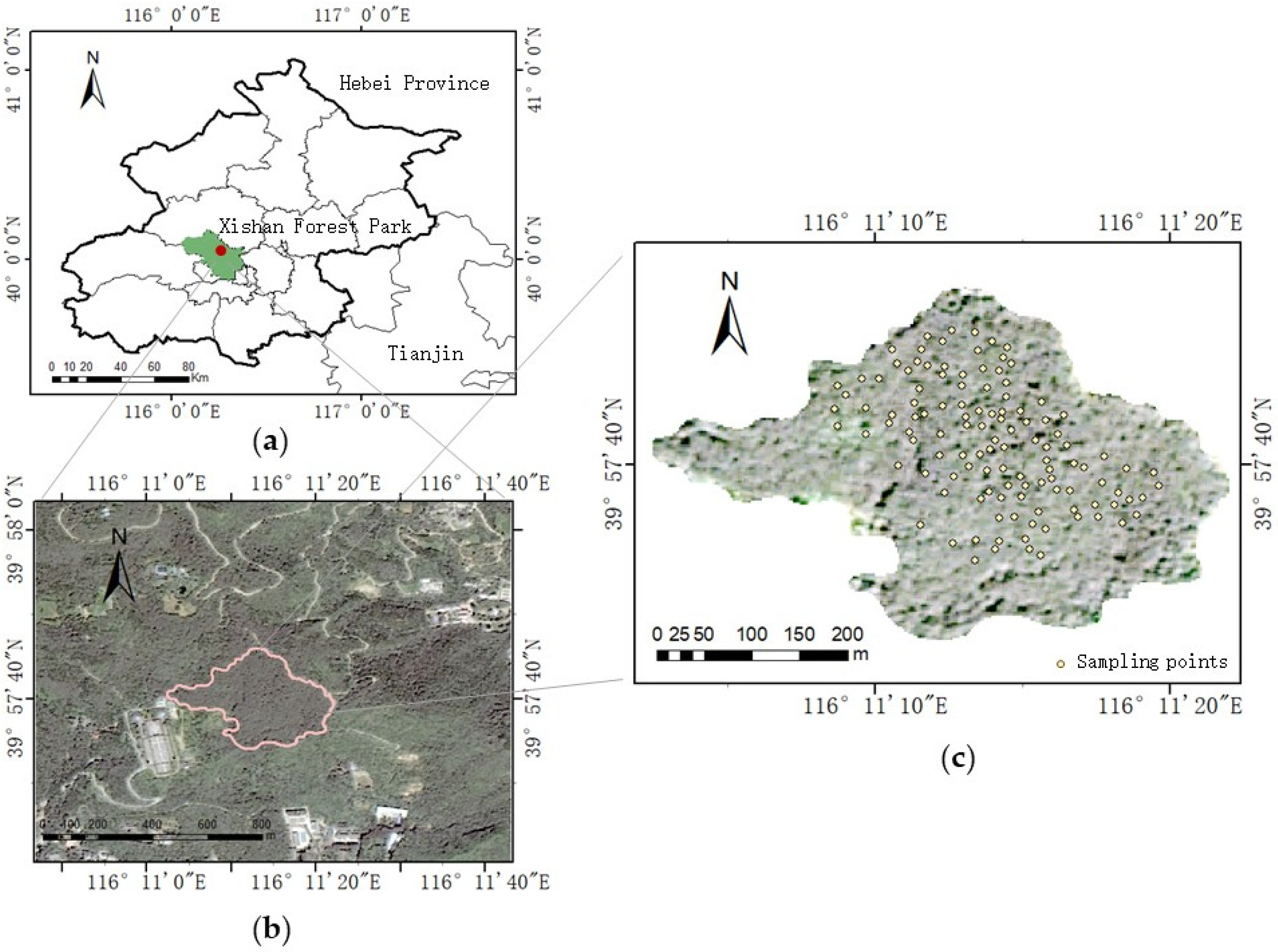
Figure 1. Xishan Forest Park (a), Location of the study area (b), and Sampling points in the site (c).
Remotesensing 16 03627 g001
Figure 2. Technical roadmap of research method. LAI, Leaf Area Index.
Remotesensing 16 03627 g002
Figure 3. Visualization scene of three-dimensional forest stands using the LESS model, vertical view (a) and aerial view (b).
Remotesensing 16 03627 g003
Figure 4. Training set (a) and testing set (b) of the Leaf Area Index (LAI) using the Random Forest model. RMSE, root mean squared error.
Remotesensing 16 03627 g004
Figure 5. Training set (a) and testing set (b) of the Leaf Area Index (LAI) using the BP Neural Network model. RMSE, root mean squared error.
Remotesensing 16 03627 g005
Figure 6. Training set (a) and testing set (b) of the Leaf Area Index (LAI) employing the XGBoost model. RMSE, root mean squared error.
Remotesensing 16 03627 g006
Figure 7. Validation set of Leaf Area Index (LAI) utilizing the Random Forest (a), BP Neural Network (b), and XGBoost (c) algorithms. RMSE, root mean squared error.
Remotesensing 16 03627 g007aRemotesensing 16 03627 g007b
Figure 8. Leaf Area Index spatial distribution maps of the Random Forest (a) and XGBoost (b) algorithms.
Remotesensing 16 03627 g008aRemotesensing 16 03627 g008b
Table 1. Parameter settings in the LESS model.
ParameterValue Size (Range)Unit
Structure coefficient (N)1.5
Water thickness (Cw)0.015cm
Chlorophyll (Cab)30, 50, 70μg·cm−2
Dry matter (Cm)0.012g·cm−2
Blade size0.01m2
Tree height (H)9.5, 12, 14m
Coronal height3.5, 5, 6m
East-west crown width3, 4.5, 5m
North-south crown width2, 4, 5.5m
Sun zenith angle SZA43.756
Sun azimuth angle SAA164.272
Skylight proportionCalculated using the 6s model
Soil reflectanceCalculated using the Gsv model
Simulated band400–900 (in steps of 1)nm
Disclaimer/Publisher’s Note: The statements, opinions and data contained in all publications are solely those of the individual author(s) and contributor(s) and not of MDPI and/or the editor(s). MDPI and/or the editor(s) disclaim responsibility for any injury to people or property resulting from any ideas, methods, instructions or products referred to in the content.