Abstract
This study investigates the application of LiDAR point cloud datasets for building segmentation through a combined approach that integrates unsupervised segmentation with evolutionary optimization. The research evaluates the extent of improvement achievable through genetic algorithm (GA) optimization for LiDAR point cloud segmentation. The unsupervised methodology encompasses preprocessing, adaptive thresholding, morphological operations, contour filtering, and terrain ruggedness analysis. A genetic algorithm was employed to fine-tune the parameters for these techniques. Critical tunable parameters, such as the interpolation method for DSM and DTM generation, scale factor for contrast enhancement, adaptive constant and block size for adaptive thresholding, kernel size for morphological operations, squareness threshold to maintain the shape of predicted objects, and terrain ruggedness index (TRI) were systematically optimized. The study presents the top ten chromosomes with optimal parameter values, demonstrating substantial improvements of 29% in the average intersection over union (IoU) score (0.775) on test datasets. These findings offer valuable insights into LiDAR-based building segmentation, highlighting the potential for increased precision and effectiveness in future applications.
1. Introduction
In recent years, the utilization of light detection and ranging (LiDAR) technology, such as the airborne laser scanner (ALS) [1,2,3], mobile laser scanner (MLS) [4], and terrestrial laser scanner (TLS) [5], has significantly advanced in various fields, including urban planning, environmental monitoring, and infrastructure management [6,7]. LiDAR data comprise elevation points known as (3D) point clouds representing the object surface and provide detailed and accurate information about the terrain and objects within the scanned area [8]. One of the critical applications of LiDAR data is building segmentation, which plays a crucial role in urban mapping [9] and disaster management [10]. The accurate segmentation of geospatial data is critical for the design and maintenance of infrastructures like power networks, wireless communication networks, hydrological planning, and sewer planning.
Building segmentation from LiDAR point clouds involves automatically identifying and delineating building structures from the scanned area [11]. The traditional methods for building segmentation often rely on manual interpretation since building typically consists of planer surfaces, but still, it is time-consuming, labor-intensive, and prone to errors, particularly in areas with complex urban landscapes or dense vegetation cover [12]. Researchers are working on supervised and unsupervised segmentation of LiDAR point clouds. In supervised segmentation, both shallow [13] and deep learning models are used for segmentation [14]. In unsupervised segmentation, LiDAR point clouds are segmented through clustering [15] and thresholding [16].
Thresholding-based methods have gained prominence among these approaches for building segmentation due to their simplicity and efficiency. Thresholding involves setting a threshold value to segment the LiDAR point cloud into building and non-building points based on specific geometric or radiometric attributes [17]. In threshold segmentation methods, the most challenging and crucial aspect lies in selecting and establishing the threshold value. Nonetheless, these methods are particularly susceptible to noise interference. Due to the extensive difference in range and coverage of ALS, TLS, and MLS, the traditional thresholding techniques may need more adaptability due to the diverse features and characteristics inherent in various sources of point cloud data. In this context, adaptive thresholding holds promise for enhancing segmentation effectiveness in point cloud analysis relative to conventional approaches. However, post-improvement is still required as thresholding may result in false positives and irregular shapes of the object.
Due to the diverse features of LiDAR data from different sources, this work selects adaptive thresholding for generalization. However, filter contours and morphological opening and closing are employed to remove false positives and improve the resultant irregular segmentation from thresholding [18]. False positive contours are identified using the terrain ruggedness index (TRI) with the help of filter contouring [19]. In contrast, determining an optimal parameter value for these four operations still remains challenging, as it depends on various factors, such as the characteristics of the LiDAR data, the complexity of the urban environment, and the size and shape of buildings. In recent years, evolutionary approaches such as genetic algorithms (GAs) have been extensively employed in many problems for optimization purposes [20,21,22]. This paper also utilizes optimization techniques such as GAs, which have been employed to automatically tune the parameters and improve the accuracy of building segmentation [23].
This article proposes a novel approach for building segmentation from LiDAR point clouds using an evolutionary genetic algorithm for optimization combined with unsupervised segmentation. The method aims to overcome the limitations of traditional thresholding-based techniques by dynamically adjusting the threshold values and other parameters based on the specific characteristics of the input data. By integrating the strengths of thresholding and genetic algorithms, our approach seeks to achieve robust and accurate building segmentation results.
In this paper, LiDAR point clouds are preprocessed and then segmented using adaptive thresholding, morphological opening, filter contours, and morphological closing. Preprocessing and unsupervised segmentation serve as a fitness function for GA. The fitness function returns the intersection over the union (IoU) value, which serves as the fitness value for the predicted mask by comparing it with the ground truth mask. The remaining GA operators are employed to maximize the fitness value.
2. Literature
Since buildings typically consist of planar surfaces, exploring plane segmentation techniques for building segmentation is logical. For instance, ref. [5] utilized a surface-growing approach to segment TLS data into planar patches and identified building footprints based on semantic attributes such as orientation and density. Similarly, ref. [24] classified points in MLS data into linear, planar, or spherical types and applied region-growing methods with specific merging rules tailored to each type. They refined the resulting segments using normalized cuts [25] and merged them for object extraction. In another study [26], buildings are extracted via region growing and projected to generate 2D wall rectangles. Building localization was then achieved through a hypothesis and selection method. At each building location, building points were distinguished from the surroundings using a min-cut-based segmentation, considering both local geometric features and shape priors.
Many studies aim to enhance efficiency in building segmentation from point-based data by shifting to voxel-based segmentation, which reduces computational costs and memory usage. Ref. [27] employed voxel segmentation and a conditional random field approach to classify voxels from TLS data. Ref. [28] divided original points into varying-sized voxels, merging similar ones to represent distinct objects. They then identified buildings by analyzing descriptors such as normal vectors and geometric shapes. Ref. [29] proposed a method using multi-scale super voxels for urban object extraction. Segmentation into super voxels formed larger segments, which were subsequently merged into meaningful objects, aiding in recognizing common urban features. Building segmentation based on voxel segmentation depends on voxel merging or segmentation rules, which may be suitable for a given application problem or data but not a generic solution.
Rather than relying on point segmentation techniques in three-dimensional space, some researchers opt to develop building segmentation techniques based on the spatial characteristics of buildings within a 2D depth grid. Since facade points projected onto a horizontal plane exhibit more concentrated contributions compared to other objects, numerous grid-based methodologies have been proposed. Ref. [30] employed a method where point clouds were projected onto a horizontal grid, and the quantity of points projected within each grid cell was termed as the density of projected points (DoPP). Grid cells exceeding a predefined DoPP threshold were identified as facade objects. In a related approach, ref. [31] constructed a Hough voting space based on points with high DoPP and employed a K-means algorithm to detect lines corresponding to different facades. Similarly, the DoPP metric was utilized for building segmentation in the subsequent research [32,33]. While this technique proves convenient and efficient, it struggles to eliminate certain non-building objects, such as street lamps, based solely on DoPP, and setting an appropriate threshold often requires extensive parameter tuning. To address this issue, ref. [34] proposed a method to calculate the DoPP by situating the lowest building of a scene at the position of the farthest building, thereby providing an intuitive meaning to the threshold. This parameter-setting approach was also adopted in other studies for building outline extraction [35,36,37]. However, a notable drawback of this method is its dependence on detailed prior knowledge of the data, including factors like the perpendicular horizontal distance between the scanner and the surface of the farthest building facade.
After DoPP, another method [38] initially divides points into grids and computes their weights based on LiDAR point distribution, creating a geo-referenced feature image using interpolation. Ultimately, it converts the extraction of street-scene objects from 3D LiDAR data into a simpler process in a 2D imagery space. Ref. [39] also utilizes the height information in the 2D image space, also known as a depth map. To eliminate the use of expert knowledge for building height or other features, ref. [40] proposed an automatic framework for building segmentation from the 3D point, composed of neighbor selection for finding the optimal neighbor based on dimensionality [41] and eigen-entropy [42], feature extraction, then selecting the best feature from the extracted feature, and at last, classification.
In recent years, RGB features have been combined and used with LiDAR 2D depth maps for both shallow [13] and deep learning models [43] for building extractions. Ref. [13] produced a boundary mask to fine-tune random forest, light GBM, and extreme GBM on combined RGB and LiDAR depth maps to improve boundary intersection over union (BIoU). This study enhances UNet, which is a U-shaped architecture, and context-transfer UNet (CT-UNet) models by integrating LiDAR data and RGB images for precise building segmentation, using intersection over union (IoU) and boundary intersection over union (BIoU) metrics. Ref. [43] modified network configurations and optimized segmentation efficiency with LiDAR data while augmented training data and batch normalization overcome overfitting. Leveraging four different backbones through transfer learning enhances segmentation convergence and parameter efficiency. Test-time augmentation (TTA) further refines the predicted masks. Augmentation techniques reveal that the ensemble model, coupled with TTA, yields superior results compared to a single model. The inclusion of LiDAR data alongside RGB images boosts the combined score by 13.33% compared to using only RGB data.
The GA has emerged as a powerful optimization technique in the field of computer vision, offering a robust and adaptive approach to solving complex problems by selecting appropriate threshold values to segment an image [44]. Adaptive thresholding is a widely used image processing technique that aims to segment an image by identifying regions of interest based on their intensity values. Adaptive thresholding is particularly useful for images with varying background illumination, as it can adjust the threshold dynamically to account for these variations [45]. One approach to improving adaptive thresholding is to optimize the parameters used in the thresholding algorithm. GAs have been explored as a means of optimizing the parameters of adaptive thresholding [46]. Genetic algorithms are a type of optimization algorithm that is inspired by the process of natural selection [47].
GA has been effectively used for multilevel thresholding of images, especially medical images, by optimizing objective functions like Otsu’s between-class variance or Kapur’s entropy [48]. GAs can optimize threshold values as well as parameters of membership functions in fuzzy thresholding methods [48]. They offer advantages over traditional thresholding techniques by providing better segmentation results, handling complex intensity distributions, and being computationally efficient for multilevel thresholding [49]. Another recent study utilizes the particle swarm optimization (PSO) algorithm for selecting the best parameters for multilevel thresholding for image segmentation along with divergence measure [50].
3. Materials and Methods
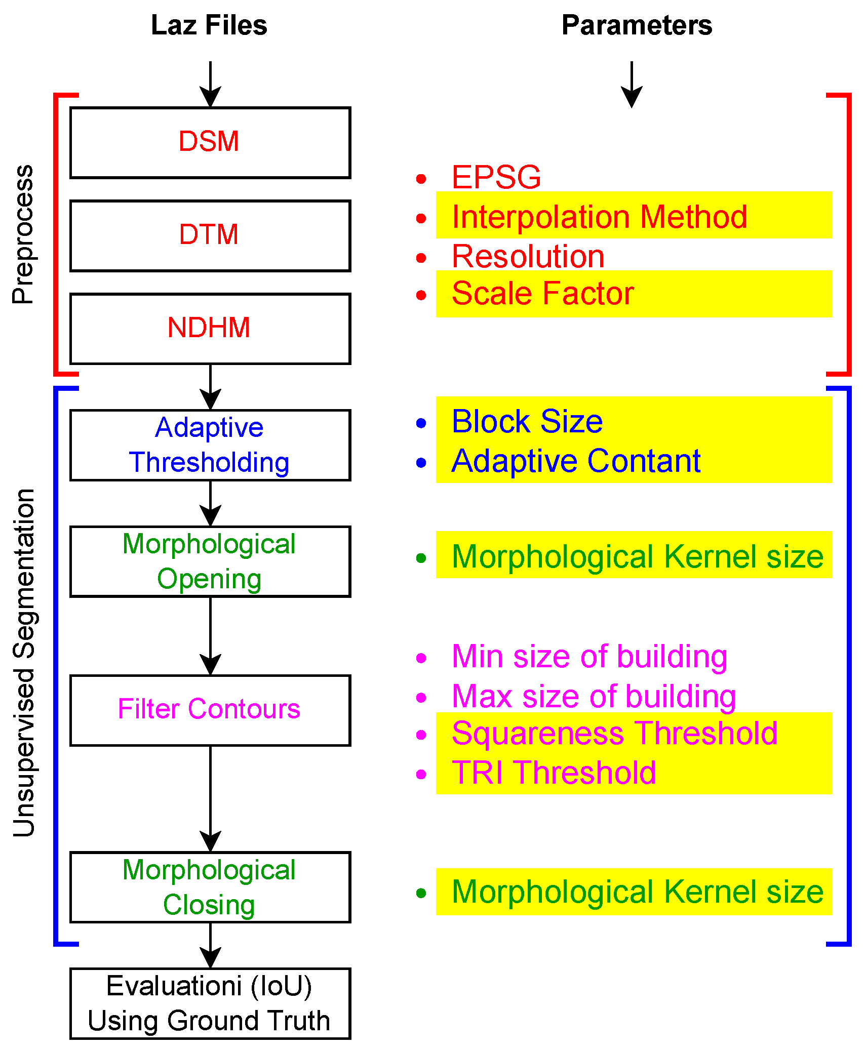
The proposed method segments LiDAR point clouds using unsupervised segmentation. The success of segmentation depends significantly on the precise tuning of its parameters, a process that is often complex and labor-intensive. To overcome this challenge, this study proposes employing genetic algorithms (GAs) to optimize the parameters of adaptive thresholding. Figure 1 illustrates the segmentation process, which serves as the fitness function for the genetic algorithm. The fitness score defines how much a chromosome is favorable; in our case, the IoU score is the fitness score. The higher the IoU, the better the chromosome or combination of parameters for segmentation in the chromosome. Section 3.2 describes the flow of the GA for the optimization of the parameters used in the segmentation process.
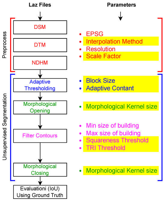
Figure 1.
Fitness function workflow diagram. The text color of functions (left) and their subsequent parameters (right) are in the same color for identification. Tunable parameters are highlighted with a yellow background, which will serve as a chromosome in the GA.
3.1. Segmentation
The fitness function consists of preprocessing and unsupervised segmentation steps, followed by IoU evaluation. DSM, DTM, and NDHM are extracted for segmentation in the preprocessing step. The segmentation procedure consists of adaptive thresholding, followed by morphological opening, filter contour, and morphological closing to the end. After segmentation, the predicted mask is evaluated using IoU, which serves as a fitness score in optimization.
Table 1 lists the optimization parameters mentioned in Figure 1 with suitable ranges as a space search for the GA. Interpolation and scale factors belong to the preprocessing step, and the remaining five parameters are block size, adaptive constant, morphological kernel, squareness threshold, and min threshold for height and width of the contours belonging to the four segmentation steps in Figure 1. Interpolation could be nearest, cubic, or linear, while scale factor is any number from a set of positive real numbers to improve pixel contrast. Block size could be an odd number in the given range. The adaptive constant should be a positive or negative number. The morphological kernel selected in the given range would be used in the morphological opening before the filter contour and morphological closing after the filter contour. The squareness threshold is a float value that shows the minimum squareness of the building that is identified. The last parameter shows the minimum threshold value for the contour in pixels. Contours having a width or height less than the threshold value would be removed.

Table 1.
Optimization parameters with search space.
3.1.1. Digital Surface Model (DSM)
This step generates a digital surface model (DSM) from the LiDAR point cloud. First, the x, y, and z coordinates of the LiDAR points are extracted from the Laz files. Next, the spatial minimum and maximum bounds of the x and y coordinates are computed to define the grid for the DSM. Then, interpolation is performed to estimate the z (elevation) values across the grid. This interpolation process can be adjusted using different methods, such as nearest neighbor, cubic, or linear interpolation. The resolution is set to 1, which corresponds to the unit of the coordinate reference system (CRS). This unit could be either meters or feet, depending on the European Petroleum Survey Group (EPSG) code, and it cannot be modified through optimization.
3.1.2. Digital Terrain Model (DTM)
The LiDAR laser pulse, when it encounters a surface such as a building roof or another object, reflects off that surface rather than penetrating to the ground. To accurately delineate building roofs and other objects on the Earth’s surface, it is necessary to separate the points that do not reflect from ground level. Fortunately, ground points are already identified in the dataset, making this step relatively straightforward.
The DTM is generated from the separated ground points using the same interpolation method and resolution as used for the DSM. The resolution parameter controls the level of detail in both the DTM and DSM. Smaller resolutions provide higher precision but potentially increase the processing time for any operation and output file size. The contrast of the pixels in the DTM can be enhanced using a scale factor, as suggested by [51]. The scale factor is another tunable parameter that can be optimized for better results.
3.1.3. Normalized Digital Height Model (NDHM)
To improve the segmentation of raw data, it is essential to normalize terrain elevation. This is achieved by calculating the normalized digital height model (NDHM), which is carried out by subtracting the ground elevation from the elevation of each point. In our case, ground elevations are represented by the DTM, while point elevations are represented by the DSM. Therefore, the NDHM is generated by subtracting the DTM from the DSM, where lower values indicate areas near the ground surface, and higher values correspond to elevated features such as buildings, trees, and other objects above ground level. By normalizing the elevation values, the influence of the terrain variation is minimized, which can significantly enhance segmentation accuracy.
3.1.4. Adaptive Thresholding
Adaptive thresholding is used to dynamically adjust the threshold value of the NDHM for noise removal and segmentation of potential building footprints. This technique depends on two parameters: block size and adaptive constant. These two parameters influence the effectiveness and granularity of adaptive thresholding, which results in the segmentation of terrain features in the LiDAR point cloud. Block size refers to the local neighborhood of the pixel, which can help to compute adaptive thresholding. NDHM is divided into small blocks, and each block’s threshold value is calculated based on the neighborhood pixel intensities within the block. The block should be an odd integer (e.g., 3 × 3, 5 × 5, 7 × 7) and chosen based on NDHM’s desired features and details. The adaptive constant is the numeric value used to enhance thresholding operations. This numeric value is subtracted from the mean computed within the block to obtain each pixel’s final adaptive threshold value. This parameter controls the sensitivity of the thresholding process: a higher value results in fewer pixels being classified as foreground. In contrast, a lower value leads to more pixels being classified as foreground. The parameter choice depends on the segmentation class and NDHM features. This step results in a binary image where the black pixel denotes ground, and the white pixel denotes buildings. However, more than thresholding is needed to conclude the results because dense vegetation reduces the efficiency of the building segmentation.
3.1.5. Morphological Opening
To further refine the thresholding results, the morphological opening is applied to separate touched objects (predicted buildings), removing small white noises (peak of the trees), and smoothing object boundaries. Morphological opening consists of erosion and dilation operations on the binary image. The kernel specifies the size and shape of the structuring element used for erosion and dilation. Kernel size determines the spatial bound over which erosion and dilation are applied to modify the binary image. Kernel size is a tunable parameter, which should be an odd number (e.g., 3 × 3, 5 × 5, 7 × 7), the small kernel size targeting and removing small noise or isolated features in the binary image. In contrast, a large kernel size influences border pixels, which could be effective for smoothing and simplifying contours. The appropriate kernel size can address challenges, irregularities, and smoothness in LiDAR data segmentation, such as differentiating vegetation and buildings, eliminating small artifacts that serve as noise, and smoothing contours of the terrain features [52].
3.1.6. Filter Contours
Filter contour serves to further smooth and refine the contour of potential building footprints. In the first step, contours are extracted from the segmented mask. Contours having an area smaller or greater than the specified limits are removed. In the second step, the squareness of the contour is determined by calculating the aspect ratio, defined as the ratio of its width to its height, as in Equation (1). For a perfect square, this aspect ratio is equal to 1. The closer the aspect ratio is to 1, the more closely the contour resembles a square. The lower the ratio, the less square the contour will be and vice versa. A contour with a squareness value less than the threshold will be removed.
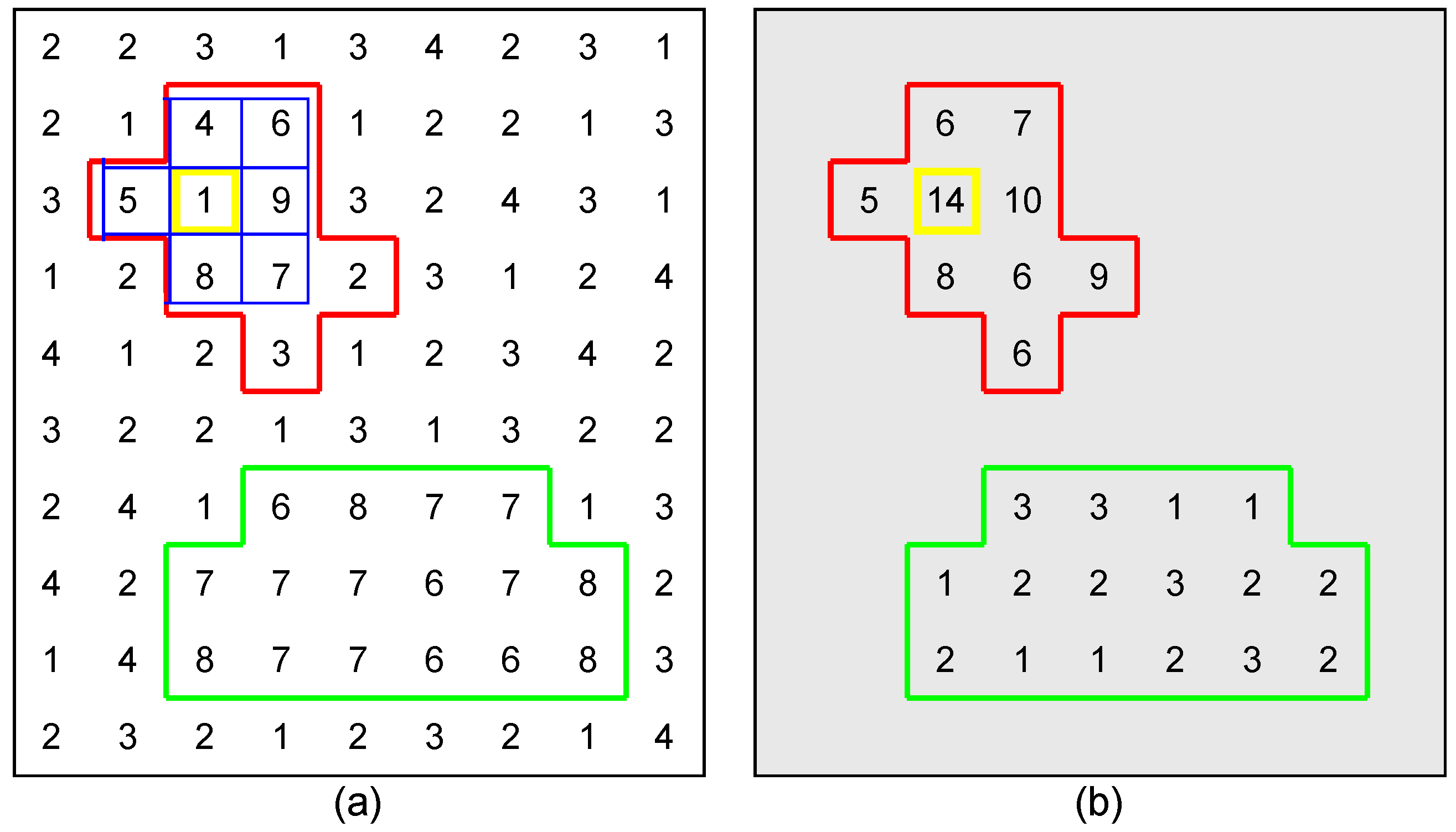
The terrain ruggedness index (TRI) helps to eliminate false positives such as trees and other objects. TRI is employed with the help of Equation (2) and illustrated using Figure 2 The terrain ruggedness index (TRI) is calculated by first selecting a central cell (yellow) and then examining its surrounding cells, typically within a 3 × 3 kernel (blue), where n is the number of pixels in the kernel. The process begins by identifying the elevation difference between the central cell and each of its eight neighboring cells . These differences are then squared to eliminate negative values and emphasize larger elevation deviations.
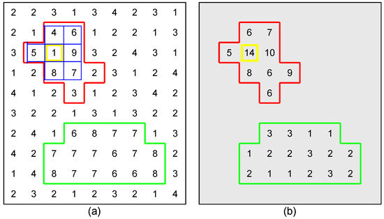
Figure 2.
TRI explanation: each DSM has a red and green contour. (a) DSM before applying Equation (2). Blue serves as a 3 × 3 kernel for contour filtering for yellow 1, as shown in example (a). (b) DSM after contour filtering. The red contour’s average value, which is TRI, is greater (not building) than the green contour (building).
Once the squared differences are computed, they are summed together to capture the overall variability in elevation around the central cell. Finally, the square root of this sum is taken to return the TRI value, which provides a single measure representing the ruggedness of the terrain in that specific area. The higher the TRI value, the more rugged the terrain, with larger elevation differences indicating greater roughness and vice versa.
Figure 2 illustrates two DSM: (a) before TRI and (b) after TRI, and each consists of two contours: blue and green. The elevation values inside contours are predicted as buildings, and the outside values are predicted as non-building. With the help of TRI, these contours will be identified as true positive or false positive. The ruggedness of each elevation value in the contours is calculated using Equation (2). The average value of the contours in (b) serves as the TRI value in the DSM. The TRI of each contour is compared with the TRI threshold value, and the contours with greater TRI are removed. In the given example, the TRI value of the red contour is higher, indicating that the contour represents a non-flat surface. In contrast, the lower TRI value of the green contour suggests it may correspond to a building.
3.1.7. Morphological Closing
Morphological closing consists of dilation and erosion. The contour image is dilated by a structuring element called a kernel to expand and fill gaps or holes within the contour boundaries. Dilation involves replacing each pixel in the image with the maximum pixel value in its neighborhood proximity defined by the kernel. This process helps bridge small breaks and reconnect parts of the contour. The dilated contour then undergoes erosion using the same structuring element. Erosion involves replacing each pixel in the image with the minimum pixel value in its neighborhood, which helps to refine and smooth the contour boundaries while preserving the overall shape. The combined effect of dilation followed by erosion in morphological closing results in closing black gaps and holes within the contours, smoothing out irregularities, and ensuring more continuous and well-defined contour shapes. This process is beneficial for improving the quality and connectivity of contours after the initial processing steps, such as TRI-based thresholding, which may have led to fragmented or incomplete contour representations.
3.1.8. Evaluation
The proposed method is validated with the help of a modified version of intersection over union (IoU) [53]. Equation (3) calculates the IoU value for the given dataset where is the union of all polygons predicted by segmentation and is the union of all polygons in the ground truth. If more polygons are predicted as compared to polygons in ground truth, then IoU is reduced with the help of Equation (4), where g denotes polygons in ground truth and p denotes polygons in prediction.
3.2. Genetic Algorithm (GA)
For accurate and reliable segmentation of buildings from aerial LiDAR data using unsupervised techniques, it is crucial to optimize the parameters across three key stages: preprocessing, thresholding, and contour filtering. The traditional methods often rely on manual tuning or heuristic approaches to set these parameters, which can be time-consuming and subjective. The evolutionary approach could be more effective and systematic for parameter optimization. Evolutionary algorithms, such as genetic algorithms (GAs), are particularly effective in this context due to the ability to efficiently navigate complex parameter spaces. They seek optimal combinations that enhance segmentation quality based on the defined objectives of the fitness function. The optimal combination search is influenced by two concepts in GA: exploitation and exploration. Exploitation refers to the process of focusing the search on areas of the solution space that are already known to be promising. Exploitation could be performed with the help of elitism as it reproduces and refines solutions that have performed well in the previous generations. On the contrary, exploration refers to the process of searching through new or less-visited regions of the solution space. The addition of new random solutions supports diversity and exploration in GA. The natural evolution operators such as crossover and mutation support both exploitation and exploration. Excess exploitation may result in premature convergence, while excess exploration results in slow convergence; therefore, balance is required. With the help of balanced exploitation and exploration, GA can effectively navigate large solution spaces through successive generations, ultimately converging toward optimal solutions. This article explores the use of GA for optimizing building segmentation parameters, demonstrating their effectiveness in enhancing the IoU score and robustness of the segmentation process.
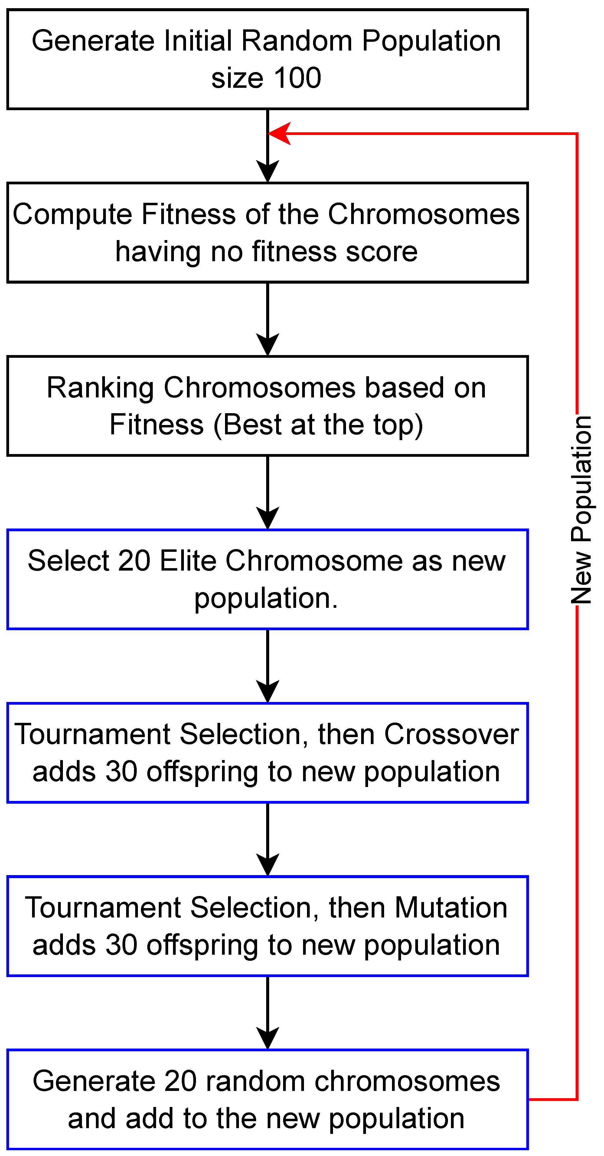
Figure 3 illustrates the flow diagram of the genetic algorithm. The process begins with the generation of a random initial population for the upcoming generation loop of GA. Inside the generation, this population serves as the current population. In the second step, the fitness score of each individual in the population is calculated using the fitness function explained in Figure 1. In the third step, the population is ranked based on these fitness scores, with the best chromosomes placed at the top. The fourth step involves passing the best 20 chromosomes to the new population, which serve in the next generation of the GA. In steps five and six, better individuals are selected, followed by crossover and mutation operations, and the offspring of these operations are added to the new population. The final step generates the remaining 20 chromosomes to complete a new population of 100 for the next generation. The final step generates the remaining 20 chromosomes to enhance exploration within the GA and complete the total of 100 chromosomes for the next generation. The algorithm is designed to operate with 100 chromosomes per generation and accumulates 100 chromosomes as the new population for the subsequent generation.
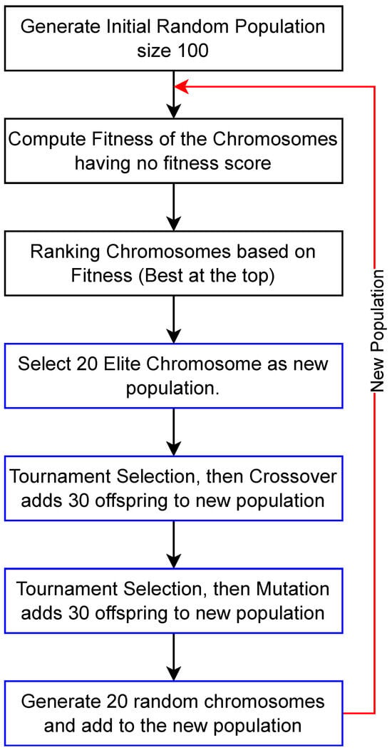
Figure 3.
Flow diagram of genetic algorithm. The red arrow denotes the generation loop. The algorithm terminates if the fitness score is the same in 10 consecutive generations.
3.2.1. Population
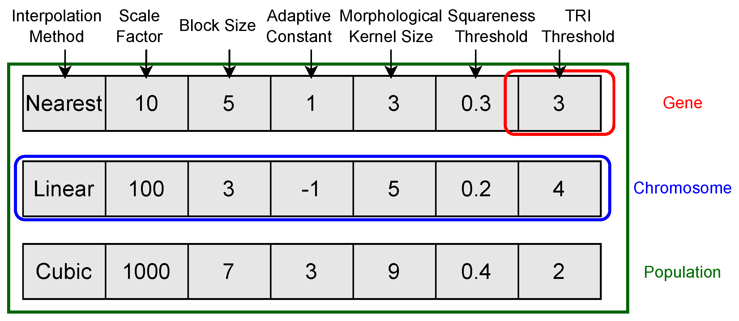
In the proposed GA for this problem, the first step involves generating a population consisting of chromosomes. A chromosome in GA represents a potential solution to the problem, which will be optimized and typically encoded as a string of genes. Each gene corresponds to a parameter or variable within a chromosome, contributing to defining a potential solution. In the context of this work, the concepts of population, chromosomes, and genes are illustrated in Figure 4.
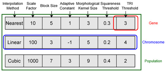
Figure 4.
Population (green), chromosomes (blue), and genes (red) are indicated with different colors for understanding.
The number of genes in the chromosome is defined by the number of parameters we want to optimize. Each chromosome consists of 7 genes, which represent parameters for optimization. The population count is defined by considering the problem context, the number of genes in the chromosomes, and the search space for each gene. A larger population is required if the search space is large, while a small search space requires a lower population. An extensive population results in fewer generations reaching the optimal solution, while a small population results in more generations seeking the optimal solution while considering the problem’s complexity. Initially, 100 chromosomes are generated by considering the search space. The first step in Figure 3 is executed only once and excluded from the generation loop of the GA.
3.2.2. Fitness Function
Figure 1 mimics the fitness function in GA explained in Section 3.1, where the Laz files and parameters are provided as input to the function. The fitness function assigns a fitness score to each chromosome in the form of IoU. This step is repeated for all generations. In the first generation, the fitness value is computed for all chromosomes since all chromosomes initially lack fitness scores. In subsequent generations, the elite chromosomes are directly transferred to the new population, retaining their previously assigned fitness scores. Consequently, fitness scores are only computed for new chromosomes (80), which are produced through crossover (30), mutation (30), and random population generation (20).
3.2.3. Ranking Chromosomes
The fitness function assigns a fitness score to all chromosomes in the population. This step ranks the chromosomes in the population based on fitness score. Chromosomes with high fitness scores are ranked at the top, and the lower ones are at the bottom. This ranking step helps in the extraction of the elite (top-ranked) chromosomes for the new population.
3.2.4. Elitism
Elitism ensures that the best solutions found so far in the current population are preserved and passed unchanged to the next generation, thereby preventing the loss of good solutions during the evolutionary process. The top 20 chromosomes from the current population are directly stored unchanged in the new population but still reside in the current population to contribute to crossover and mutation operations. The 20 elite chromosomes transferred to the new population serve two main purposes. First, they ensure that the best solutions found so far are preserved during the evolutionary process to support exploitation. Second, tournament selection is used to choose individuals for crossover and mutation. If insufficient elite chromosomes are stored in the new population (e.g., 5), they might not be chosen by tournament selection in the next generation due to the small sample size, which reduces exploitation. Conversely, if too many elite chromosomes are stored (e.g., 50, which is half of the population), tournament selection may favor them too strongly, leading to increased exploitation but reduced exploration. To address these issues, 20 elite chromosomes are stored in the new population and tested through tournament selection among a population of 100. This approach helps maintain a balance between exploitation and exploration by ensuring that selected individuals come from both elite chromosomes and the new offspring generated through crossover and mutation in the previous generations.
3.2.5. Crossover
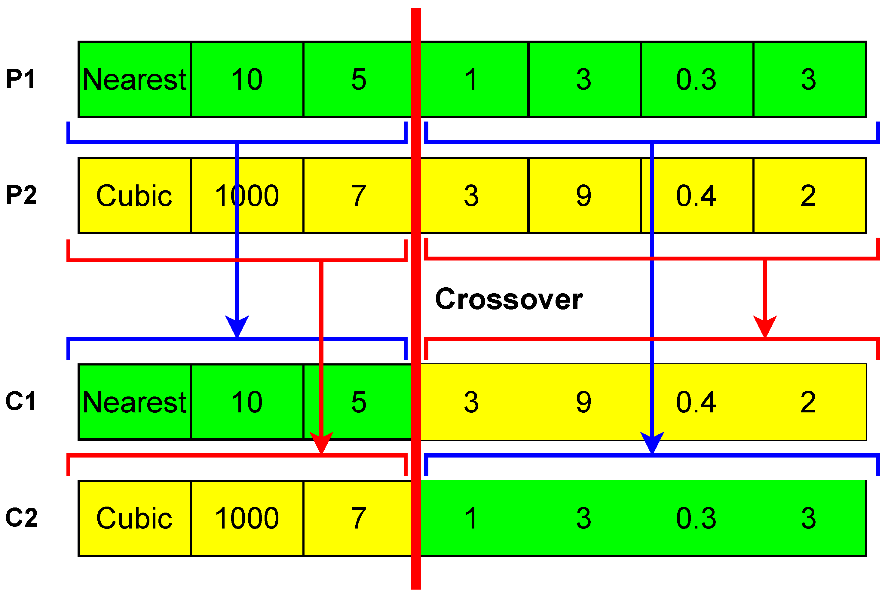
Tournament selection is used to select parents from the current population for the crossover. The process involves randomly selecting a subset of individuals from the current population and then choosing the best individual within the subset, on the basis of fitness/IoU, to be a parent for producing offspring. A subset of three individuals is randomly selected from the current population, and then, an individual with high fitness is selected from the subset. Figure 5 shows two selected parents through tournament selection as and , and then a random cut is drawn on both parents. The left side of from the cut is connected with the right side of from the cut to produce child . The remaining parts from both parents are connected for . In this way, the crossover is performed 15 times; each time, two parents are selected from the current population through tournament selection, which results in two offspring; hence, 30 offspring are produced and added to the new population.
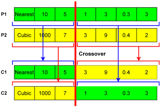
Figure 5.
Crossover of two parents. and are two parents, the Red straight line determines the cut on the parents, and and are two offspring/children producers through the crossover.
3.2.6. Mutation
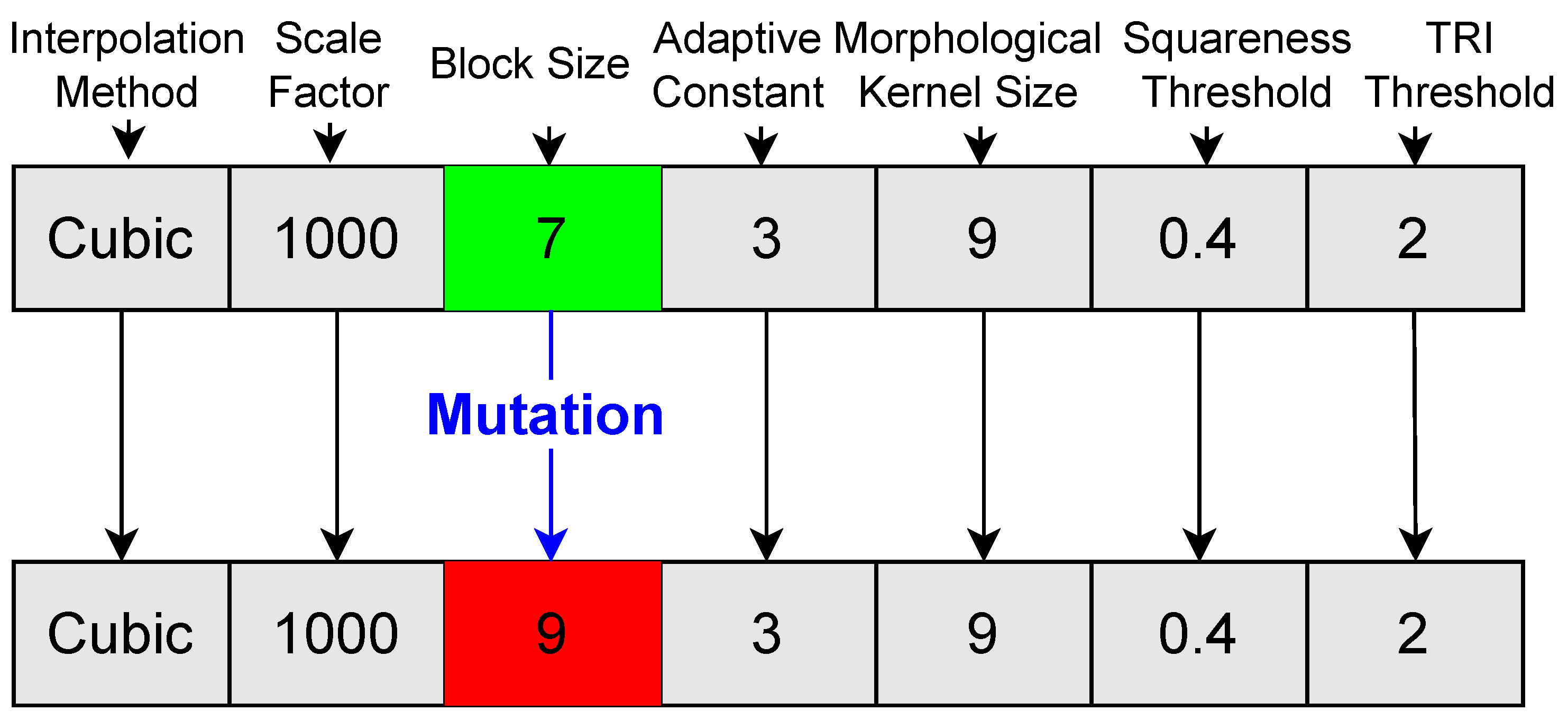
A mutation is a genetic operator used in GAs to introduce variations in the genes of individuals within a population. The purpose of mutation is to maintain genetic diversity and explore new areas of the solution space that may not be reachable through crossover alone. The tournament selection procedure is employed to select parents from the current population for mutation. Figure 6 represents the mutation operator, in which a selected parent goes through mutation. In the mutation process, a gene is randomly selected (green) and changed according to the parameter range (red) mentioned in Table 1 for exploration. In the given example, the block size gene is randomly selected and changed to another odd value according to the block size range rather than any random number. In the case of the interpolation method, if selected for mutation, the value should be changed from cubic to linear or nearest.
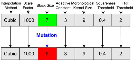
Figure 6.
Mutation of an individual in which the third gene is randomly selected and altered for diversity.
4. Results
4.1. Dataset
This work uses the same dataset as the 11th SIGSPATIAL Cup Competition (GIS CUP 2022), consisting of LiDAR point cloud datasets captured by the 3D elevation program (3DEP) [54] and provided by the United States Geological Survey (USGS) [55]. The competition focuses on analyzing large datasets where each dataset is composed of a dense array of points, and each point represents its height. Ten datasets are available on the competition website, with LiDAR point clouds and ground truth. The LiDAR point cloud dataset is provided as Laz files, and ground truth is provided in GeoJSON format. The GeoJSON file consists of building boundaries as polygons. The proposed method also returns a set of polygons that represent the perimeter of the detected building. Multiple polygons should not cover one building, and one polygon should not cover multiple buildings. The IoU score is penalized for the positive prediction of polygons. The Laz file is provided for the preprocessing step for generating the DSM and DTM. In the segmentation step, buildings are extracted from the preprocessed DSM, and the contour of the predicted building is stored in the predicted GeoJSON, which is later compared with ground truth GeoJSON.
4.2. IoU Comparison
Table 2 lists the dataset files with the dataset number used in the websites, EPSG value evaluated for datasets through QGIS application, and location of the dataset, and the proposed results are compared with [56]. The first six files (0, 4, 6, 7, 8, 9) are used for the training set, and the remaining four files (10, 11, 13, 16) are used for the testing set. The average IoU for the test sets by [56] is 0.485, and the proposed work is 0.775, which results in a 29% improvement. The proposed work shows promising results on all dataset files, including training and testing files.

Table 2.
Results comparison on the same datasets. Blue dataset numbers are used for training while red are used for testing.
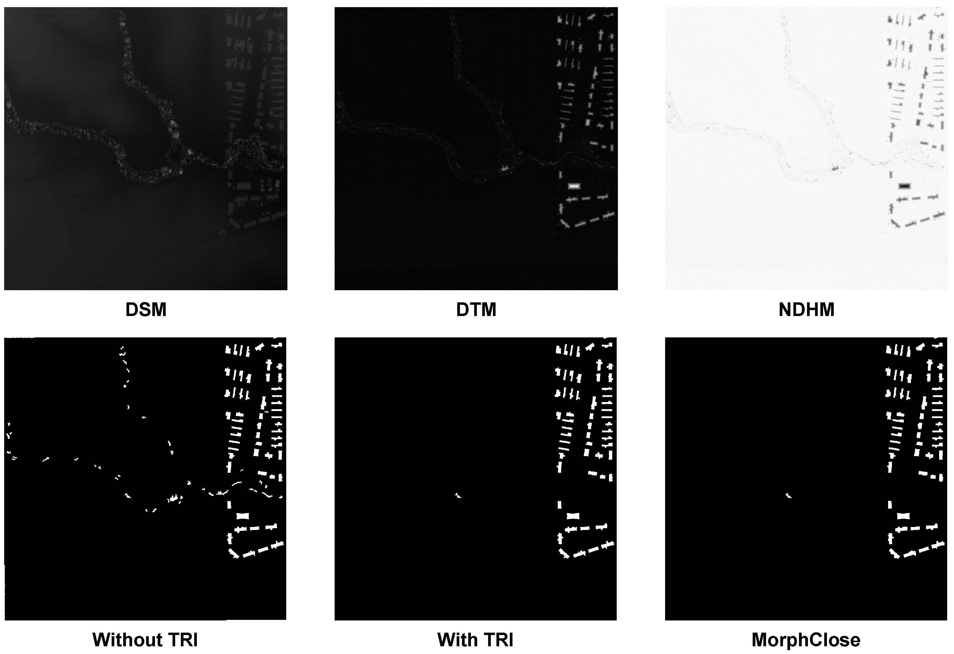
Figure 7 presents the results for dataset file 11, depicting a subset of land from Illinois. The top row in the figure displays the DSM, DTM, and NDHM images generated during the preprocessing step of the fitness function. The third image in the first row is the NDHM, where the terrain is absent, and only objects above the earth’s surface are highlighted. The NDHM reveals that buildings are on the right side, and zigzag lines of trees are on the left side.

Figure 7.
Dataset 11th Illinois result, first row results from preprocessing step and second-row results from segmentation.
The first image in the second row shows the segmentation result without applying the TRI concept, where both buildings and trees are segmented, leading to false segmentation. The second row of images illustrates the segmentation outcome using the TRI concept. Here, trees are successfully excluded except for three white contours, which are misidentified as trees. These contours were excluded because their average TRI was high due to the characteristics of the tree structures. The final image in the second row shows the segmentation results after applying a morphological close operation, which further refines the contours of the segmented buildings.
4.3. Convergence Curve
The convergence graph in Figure 8 illustrates the evolution of the population’s fitness over successive generations. The average IoU is used as a fitness score for evolution. The graph explicitly depicts the fitness value of the best chromosome in the population for each generation. Due to the application of elitism, where the top 20 chromosomes are retained in each generation, the fitness value never decreases, resulting in a non-descending graph. The horizontal straight line observed in the graph indicates that the top fitness value remains constant across these generations, likely representing the final generations where no further improvement occurs.
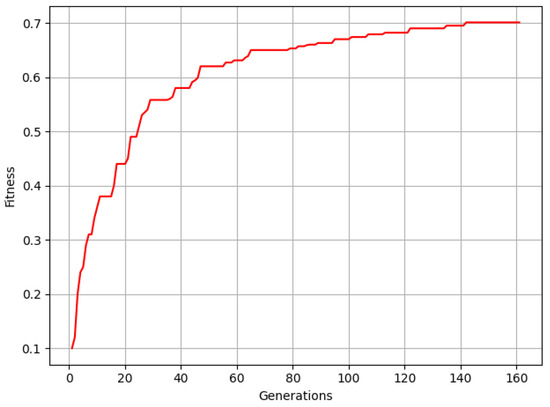
Figure 8.
Genetic Algorithm (GA) Convergence Graph: The Y-axis represents the fitness score (IoU) of the top chromosome, while the X-axis indicates the generation number at which the top fitness score was achieved.
5. Discussion
Table 3 shows the top 10 chromosomes with the best IoU scores. Despite being utilized by [57,58], we endeavored to assess the optimal interpolation method, whether nearest, cubic, or linear, using a GA. This study suggests that the nearest neighbor is the best. It maintains sharp boundaries of features like buildings and trees better than linear or cubic interpolation, which tend to smooth transitions. Nearest neighbor interpolation is also less sensitive to noise and computationally less intensive, allowing for faster evaluations and better optimization results during the GA process.

Table 3.
Top 10 elite chromosomes with IoU score after 100 generation of GA.
According to [51], the scale factor is used to determine the multi-scale solution for DSM generation. The empirical optimization in the proposed work suggests a higher scale factor of 1100 for LiDAR point cloud segmentation datasets. This effectively balances the contrast and differentiation of features, enhancing the accuracy of segmenting various features such as buildings, trees, and ground. This value likely distributes data values across a dynamic range, making subtle differences in elevation more apparent and easier to segment.
Larger block sizes help in averaging noise; on the contrary, small block sizes might be too sensitive to minor variations and noise. The top 10 chromosomes usually have 127, 129, 133, and 135 values, which is relatively large, which means that it includes a significant number of pixels in the computation of the local threshold. This helps in capturing broader local variations in lighting and texture. The genetic algorithm sorts out a large block size due to the objective and region of interest in the LiDAR point cloud, which is buildings that are relatively big objects.
The block size is related to adaptive thresholding.
Larger values of the adaptive constant might either miss important details or introduce too much noise, whereas the small values provide a good balance. The adaptive constant in the top 10 chromosomes is either −1, 0, or 1 as the best adaptive constant value for the given datasets. These low values of the constant for the LiDAR point cloud show that the variability in the point cloud is quite low and uniform. The real-world dataset often required minute adjustments to overcome local variability.
The optimal kernel size is 5 for morphological opening and closing in LiDAR point cloud segmentation for the given datasets, effectively balancing noise removal and feature preservation. It sufficiently removes small noise artifacts like cars, electricity poles, etc., without affecting larger structures like buildings, using erosion to eliminate isolated points and dilation to restore larger shapes. This size is large enough to smooth the boundaries of buildings and ground surfaces while maintaining their integrity and shape. Morphological operations with a kernel size of 5 improve segmentation by reducing jagged edges and ensuring uniform boundaries, striking a balance between the noise reduction and detail preservation tailored to the dataset’s needs.
A TRI threshold of 5 effectively distinguishes terrain characteristics relevant to buildings by identifying abrupt changes in terrain, indicating potential building footprints or boundaries. This sensitivity captures distinct elevation changes typical of buildings while minimizing noise and variations that could affect segmentation accuracy. This threshold is particularly suitable for urban environments where the buildings’ unique elevation profiles are prominent and easily distinguishable, facilitating precise segmentation and analysis.
6. Conclusions
This research demonstrates the effectiveness of using LiDAR point cloud datasets for building segmentation through a combined approach incorporating unsupervised segmentation techniques and genetic algorithm optimization. The methods employed include generating DSM, DTM, and NDHM, adaptive thresholding, morphological opening, contour filtering, terrain ruggedness, and morphological opening, each contributing to the accurate delineation of features. The optimization of parameters related to these techniques was achieved using a genetic algorithm, ensuring the best possible outcomes for segmentation. Key tunable parameters such as the interpolation method for DSM generation, scale factor for contrast enhancement, adaptive constant and block size for adaptive thresholding, kernel size for morphological operations, and TRI thresholding were carefully adjusted. The results highlight the top ten chromosomes, presenting the optimal values for these parameters and underscoring the robustness and precision of the proposed methodology. This study offers significant insights and advancements in the field of LiDAR-based building segmentation, paving the way for further improvements and applications.
Author Contributions
Conceptualization, M.S. and C.R.; methodology, M.S. and M.F.; software, M.S.; validation, M.S.; formal analysis, M.S. and A.N.B.; investigation, M.S.; resources, A.N.B. and C.R.; data curation, M.S.; writing—original draft preparation, M.S.; writing—review and editing, M.S.; visualization, M.S.; supervision, C.R.; project administration, A.N.B.; funding acquisition, C.R. All authors have read and agreed to the published version of the manuscript.
Funding
This work is supported by the project EMB3DCAM, “Next Generation 3D Machine Vision with Embedded Visual Computing,” and is co-funded under grant number 325748 of the Research Council of Norway.
Data Availability Statement
The dataset used in this work is available at https://sigspatial2022.sigspatial.org/giscup/index.html (accessed on 11 September 2024).
Conflicts of Interest
The authors declare no conflicts of interest.
References
- Tomljenovic, I.; Höfle, B.; Tiede, D.; Blaschke, T. Building extraction from airborne laser scanning data: An analysis of the state of the art. Remote Sens. 2015, 7, 3826–3862. [Google Scholar] [CrossRef]
- Lai, X.; Yang, J.; Li, Y.; Wang, M. A building extraction approach based on the fusion of LiDAR point cloud and elevation map texture features. Remote Sens. 2019, 11, 1636. [Google Scholar] [CrossRef]
- Du, S.; Zhang, Y.; Zou, Z.; Xu, S.; He, X.; Chen, S. Automatic building extraction from LiDAR data fusion of point and grid-based features. ISPRS J. Photogramm. Remote Sens. 2017, 130, 294–307. [Google Scholar] [CrossRef]
- Che, E.; Jung, J.; Olsen, M.J. Object recognition, segmentation, and classification of mobile laser scanning point clouds: A state of the art review. Sensors 2019, 19, 810. [Google Scholar] [CrossRef]
- Pu, S.; Vosselman, G. Knowledge based reconstruction of building models from terrestrial laser scanning data. ISPRS J. Photogramm. Remote Sens. 2009, 64, 575–584. [Google Scholar] [CrossRef]
- Debnath, S.; Paul, M.; Debnath, T. Applications of LiDAR in agriculture and future research directions. J. Imaging 2023, 9, 57. [Google Scholar] [CrossRef] [PubMed]
- Li, S.; Dai, L.; Wang, H.; Wang, Y.; He, Z.; Lin, S. Estimating leaf area density of individual trees using the point cloud segmentation of terrestrial LiDAR data and a voxel-based model. Remote Sens. 2017, 9, 1202. [Google Scholar] [CrossRef]
- Yang, H.L.; Yuan, J.; Lunga, D.; Laverdiere, M.; Rose, A.; Bhaduri, B. Building extraction at scale using convolutional neural network: Mapping of the united states. IEEE J. Sel. Top. Appl. Earth Obs. Remote Sens. 2018, 11, 2600–2614. [Google Scholar] [CrossRef]
- Ghanea, M.; Moallem, P.; Momeni, M. Building extraction from high-resolution satellite images in urban areas: Recent methods and strategies against significant challenges. Int. J. Remote Sens. 2016, 37, 5234–5248. [Google Scholar] [CrossRef]
- Hu, Q.; Zhen, L.; Mao, Y.; Zhou, X.; Zhou, G. Automated building extraction using satellite remote sensing imagery. Autom. Constr. 2021, 123, 103509. [Google Scholar] [CrossRef]
- Wang, R.; Peethambaran, J.; Chen, D. Lidar point clouds to 3D urban models: A review. IEEE J. Sel. Top. Appl. Earth Obs. Remote Sens. 2018, 11, 606–627. [Google Scholar] [CrossRef]
- Wang, B.; Wu, V.; Wu, B.; Keutzer, K. Latte: Accelerating lidar point cloud annotation via sensor fusion, one-click annotation, and tracking. In Proceedings of the 2019 IEEE Intelligent Transportation Systems Conference (ITSC), Auckland, New Zealand, 27–30 October 2019; pp. 265–272. [Google Scholar]
- Sulaiman, M.; Farmanbar, M.; Belbachir, A.N.; Rong, C. Precision in Building Extraction: Comparing Shallow and Deep Models Using LiDAR Data. In Frontiers of Artificial Intelligence, Ethics, and Multidisciplinary Applications; Springer: Berlin/Heidelberg, Germany, 2023; pp. 431–444. [Google Scholar]
- Zhang, J.; Zhao, X.; Chen, Z.; Lu, Z. A review of deep learning-based semantic segmentation for point cloud. IEEE Access 2019, 7, 179118–179133. [Google Scholar] [CrossRef]
- Zhao, Y.; Zhang, X.; Huang, X. A technical survey and evaluation of traditional point cloud clustering methods for lidar panoptic segmentation. In Proceedings of the IEEE/CVF International Conference on Computer Vision, Montreal, BC, Canada, 11–17 October 2021; pp. 2464–2473. [Google Scholar]
- Ma, L.; Li, Y.; Li, J.; Wang, C.; Wang, R.; Chapman, M.A. Mobile laser scanned point-clouds for road object detection and extraction: A review. Remote Sens. 2018, 10, 1531. [Google Scholar] [CrossRef]
- Chen, M.; Liu, X.; Zhang, X.; Wang, M.; Zhao, L. Building extraction from terrestrial laser scanning data with density of projected points on polar grid and adaptive threshold. Remote Sens. 2021, 13, 4392. [Google Scholar] [CrossRef]
- Said, K.A.M.; Jambek, A.B.; Sulaiman, N. A study of image processing using morphological opening and closing processes. Int. J. Control Theory Appl. 2016, 9, 15–21. [Google Scholar]
- Różycka, M.; Migoń, P.; Michniewicz, A. Topographic Wetness Index and Terrain Ruggedness Index in geomorphic characterisation of landslide terrains, on examples from the Sudetes, SW Poland. Z. Geomorphol. Suppl. Issues 2017, 61, 61–80. [Google Scholar] [CrossRef]
- Sulaiman, M.; Halim, Z.; Lebbah, M.; Waqas, M.; Tu, S. An evolutionary computing-based efficient hybrid task scheduling approach for heterogeneous computing environment. J. Grid Comput. 2021, 19, 1–31. [Google Scholar] [CrossRef]
- Halim, Z.; Yousaf, M.N.; Waqas, M.; Sulaiman, M.; Abbas, G.; Hussain, M.; Ahmad, I.; Hanif, M. An effective genetic algorithm-based feature selection method for intrusion detection systems. Comput. Secur. 2021, 110, 102448. [Google Scholar] [CrossRef]
- Mustafa, G.; Rauf, A.; Al-Shamayleh, A.S.; Sulaiman, M.; Alrawagfeh, W.; Afzal, M.T.; Akhunzada, A. Optimizing document classification: Unleashing the power of genetic algorithms. IEEE Access 2023, 11, 83136–83149. [Google Scholar] [CrossRef]
- Wang, Z.; Wang, Y.; Jiang, L.; Zhang, C.; Wang, P. An image segmentation method using automatic threshold based on improved genetic selecting algorithm. Autom. Control Comput. Sci. 2016, 50, 432–440. [Google Scholar] [CrossRef]
- Yang, B.; Dong, Z. A shape-based segmentation method for mobile laser scanning point clouds. ISPRS J. Photogramm. Remote Sens. 2013, 81, 19–30. [Google Scholar] [CrossRef]
- Shi, J.; Malik, J. Normalized cuts and image segmentation. IEEE Trans. Pattern Anal. Mach. Intell. 2000, 22, 888–905. [Google Scholar]
- Xia, S.; Wang, R. Extraction of residential building instances in suburban areas from mobile LiDAR data. ISPRS J. Photogramm. Remote Sens. 2018, 144, 453–468. [Google Scholar] [CrossRef]
- Lim, E.H.; Suter, D. 3D terrestrial LIDAR classifications with super-voxels and multi-scale Conditional Random Fields. Comput.-Aided Des. 2009, 41, 701–710. [Google Scholar] [CrossRef]
- Aijazi, A.K.; Checchin, P.; Trassoudaine, L. Segmentation based classification of 3D urban point clouds: A super-voxel based approach with evaluation. Remote Sens. 2013, 5, 1624–1650. [Google Scholar] [CrossRef]
- Yang, B.; Dong, Z.; Zhao, G.; Dai, W. Hierarchical extraction of urban objects from mobile laser scanning data. ISPRS J. Photogramm. Remote Sens. 2015, 99, 45–57. [Google Scholar] [CrossRef]
- Li, B.; Li, Q.; Shi, W.; Wu, F. Feature extraction and modeling of urban building from vehicle-borne laser scanning data. Int. Arch. Photogramm. Remote Sens. Spat. Inf. Sci 2004, 35, 934–939. [Google Scholar]
- Hammoudi, K.; Dornaika, F.; Paparoditis, N. Extracting building footprints from 3D point clouds using terrestrial laser scanning at street level. ISPRS/CMRT09 2009, 38, 65–70. [Google Scholar]
- Fan, H.; Yao, W.; Tang, L. Identifying man-made objects along urban road corridors from mobile LiDAR data. IEEE Geosci. Remote Sens. Lett. 2013, 11, 950–954. [Google Scholar] [CrossRef]
- Hernández, J.; Marcotegui, B. Point cloud segmentation towards urban ground modeling. In Proceedings of the 2009 Joint Urban Remote Sensing Event, Shanghai, China, 20–22 May 2009; pp. 1–5. [Google Scholar]
- Cheng, L.; Tong, L.; Wu, Y.; Chen, Y.; Li, M. Shiftable leading point method for high accuracy registration of airborne and terrestrial LiDAR data. Remote Sens. 2015, 7, 1915–1936. [Google Scholar] [CrossRef]
- Zheng, H.; Wang, R.; Xu, S. Recognizing street lighting poles from mobile LiDAR data. IEEE Trans. Geosci. Remote Sens. 2016, 55, 407–420. [Google Scholar] [CrossRef]
- Cheng, L.; Tong, L.; Li, M.; Liu, Y. Semi-automatic registration of airborne and terrestrial laser scanning data using building corner matching with boundaries as reliability check. Remote Sens. 2013, 5, 6260–6283. [Google Scholar] [CrossRef]
- Cheng, X.; Cheng, X.; Li, Q.; Ma, L. Automatic registration of terrestrial and airborne point clouds using building outline features. IEEE J. Sel. Top. Appl. Earth Obs. Remote Sens. 2018, 11, 628–638. [Google Scholar] [CrossRef]
- Yang, B.; Wei, Z.; Li, Q.; Li, J. Automated extraction of street-scene objects from mobile lidar point clouds. Int. J. Remote Sens. 2012, 33, 5839–5861. [Google Scholar] [CrossRef]
- Gao, S.; Hu, Q. Automatic extraction method of independent features based on elevation projection of point clouds and morphological characters of ground object. In Proceedings of the 2014 Third International Workshop on Earth Observation and Remote Sensing Applications (EORSA), Changsha, China, 11–14 June 2014; pp. 86–90. [Google Scholar]
- Weinmann, M.; Jutzi, B.; Hinz, S.; Mallet, C. Semantic point cloud interpretation based on optimal neighborhoods, relevant features and efficient classifiers. ISPRS J. Photogramm. Remote Sens. 2015, 105, 286–304. [Google Scholar] [CrossRef]
- Demantké, J.; Mallet, C.; David, N.; Vallet, B. Dimensionality based scale selection in 3D lidar point clouds. Int. Arch. Photogramm. Remote Sens. Spat. Inf. Sci. 2012, 38, 97–102. [Google Scholar] [CrossRef]
- Weinmann, M.; Jutzi, B.; Mallet, C. Semantic 3D scene interpretation: A framework combining optimal neighborhood size selection with relevant features. ISPRS Ann. Photogramm. Remote Sens. Spat. Inf. Sci. 2014, 2, 181–188. [Google Scholar] [CrossRef]
- Sulaiman, M.; Finnesand, E.; Farmanbar, M.; Belbachir, A.N.; Rong, C. Building Precision: Efficient Encoder-Decoder Networks for Remote Sensing based on Aerial RGB and LiDAR data. IEEE Access 2024, 12, 60329–60346. [Google Scholar] [CrossRef]
- Manikandan, S.; Ramar, K.; Iruthayarajan, M.W.; Srinivasagan, K. Multilevel thresholding for segmentation of medical brain images using real coded genetic algorithm. Measurement 2014, 47, 558–568. [Google Scholar] [CrossRef]
- Hsing, T.R. Techniques of adaptive threshold setting for document scanning applications. Opt. Eng. 1984, 23, 288–293. [Google Scholar] [CrossRef]
- Yu, W.; Huang, M.; Zhu, D.; Li, X. A method of image segmentation based on improved adaptive genetic algorithm. In Proceedings of the Foundations of Intelligent Systems: Proceedings of the Sixth International Conference on Intelligent Systems and Knowledge Engineering (ISKE2011), Shanghai, China, 15–17 December 2011; Springer: Berling/Heidelberg, Germany, 2012; pp. 507–516. [Google Scholar]
- Cuevas, E.; Zaldívar, D.; Perez-Cisneros, M. Applications of Evolutionary Computation in Image Processing and Pattern Recognition; Springer: Berling/Heidelberg, Germany, 2016; Volume 100. [Google Scholar]
- Hilali-Jaghdam, I.; Ishak, A.B.; Abdel-Khalek, S.; Jamal, A. Quantum and classical genetic algorithms for multilevel segmentation of medical images: A comparative study. Comput. Commun. 2020, 162, 83–93. [Google Scholar] [CrossRef]
- Houssein, E.H.; Mohamed, G.M.; Ibrahim, I.A.; Wazery, Y.M. An efficient multilevel image thresholding method based on improved heap-based optimizer. Sci. Rep. 2023, 13, 9094. [Google Scholar] [CrossRef] [PubMed]
- Nie, F.; Liu, M.; Zhang, P. Multilevel thresholding with divergence measure and improved particle swarm optimization algorithm for crack image segmentation. Sci. Rep. 2024, 14, 7642. [Google Scholar] [CrossRef] [PubMed]
- Vu, T.T.; Yamazaki, F.; Matsuoka, M. Multi-scale solution for building extraction from LiDAR and image data. Int. J. Appl. Earth Obs. Geoinf. 2009, 11, 281–289. [Google Scholar] [CrossRef]
- Sepriana, D.; Adi, K.; Widodo, C.E. CE, Application of morphological operations for improvement the segmentation image of chicken intestinal goblet cells. Int. J. Comput. Appl. 2019, 975, 8887. [Google Scholar]
- Cho, Y.J. Weighted Intersection over Union (wIoU): A New Evaluation Metric for Image Segmentation. arXiv 2021, arXiv:2107.09858. [Google Scholar]
- U.S. Geological Survey. 3D Elevation Program. Available online: https://www.usgs.gov/3d-elevation-program (accessed on 11 September 2024).
- Woods, R., Jr. ACM SIGSPATIAL Cup 2022. Available online: https://sigspatial2022.sigspatial.org/giscup/organizer.html (accessed on 11 September 2024).
- Erdem, M.; Anbaroglu, B. Reproducible Extraction of Building Footprints from Airborne LiDAR Data: A Demo Paper. In Proceedings of the 31st ACM International Conference on Advances in Geographic Information Systems, Hamburg, Germany, 13–16 November 2023; pp. 1–4. [Google Scholar]
- Song, H.; Jung, J. Challenges in building extraction from airborne LiDAR data: Ground-truth, building boundaries, and evaluation metrics. In Proceedings of the 30th International Conference on Advances in Geographic Information Systems, Seattle, WA, USA, 1–4 November 2022; pp. 1–4. [Google Scholar]
- Song, H.; Jung, J. A new explainable DTM generation algorithm with airborne LIDAR data: Grounds are smoothly connected eventually. arXiv 2022, arXiv:2208.11243. [Google Scholar]
Disclaimer/Publisher’s Note: The statements, opinions and data contained in all publications are solely those of the individual author(s) and contributor(s) and not of MDPI and/or the editor(s). MDPI and/or the editor(s) disclaim responsibility for any injury to people or property resulting from any ideas, methods, instructions or products referred to in the content. |
© 2024 by the authors. Licensee MDPI, Basel, Switzerland. This article is an open access article distributed under the terms and conditions of the Creative Commons Attribution (CC BY) license (https://creativecommons.org/licenses/by/4.0/).

