Article

Estimating Chlorophyll-a and Phycocyanin Concentrations in Inland Temperate Lakes across New York State Using Sentinel-2 Images: Application of Google Earth Engine for Efficient Satellite Image Processing

by
Sara Akbarnejad Nesheli
1,
Lindi J. Quackenbush
1,* and
Lewis McCaffrey
2
1
Department of Environmental Resources Engineering, State University of New York College of Environmental Science and Forestry (ESF), Syracuse, NY 13210, USA
2
New York State Department of Environmental Conservation (NYSDEC), Syracuse, NY 13214, USA
*
Author to whom correspondence should be addressed.
Remote Sens. 2024, 16(18), 3504; https://doi.org/10.3390/rs16183504
Submission received: 29 July 2024 / Revised: 9 September 2024 / Accepted: 19 September 2024 / Published: 21 September 2024
(This article belongs to the Section Engineering Remote Sensing)

Abstract

:
Harmful algae blooms (HABs) have been reported with greater frequency in lakes across New York State (NYS) in recent years. In situ sampling is used to assess water quality, but such observations are time intensive and therefore practically limited in their spatial extent. Previous research has used remote sensing imagery to estimate phytoplankton pigments (typically chlorophyll-a or phycocyanin) as HAB indicators. The primary goal of this study was to validate a remote sensing-based method to estimate cyanobacteria concentrations at high temporal (5 days) and spatial (10–20 m) resolution, to allow identification of lakes across NYS at a significant risk of algal blooms, thereby facilitating targeted field investigations. We used Google Earth Engine (GEE) as a cloud computing platform to develop an efficient methodology to process Sentinel-2 image collections at a large spatial and temporal scale. Our research used linear regression to model the correlation between in situ observations of chlorophyll-a (Chl-a) and phycocyanin and indices derived from Sentinel-2 data to evaluate the potential of remote sensing-derived inputs for estimating cyanobacteria concentrations. We tested the performance of empirical models based on seven remote-sensing-derived indices, two in situ measurements, two cloud mitigation approaches, and three temporal sampling windows across NYS lakes for 2019 and 2020. Our best base model (R2 of 0.63), using concurrent sampling data and the ESA cloud masking—i.e., the QA60 bitmask—approach, related the maximum peak height (MPH) index to phycocyanin concentrations. Expanding the temporal match using a one-day time window increased the available training dataset size and improved the fit of the linear regression model (R2 of 0.71), highlighting the positive impact of increasing the training dataset on model fit. Applying the Cloud Score+ method for filtering cloud and cloud shadows further improved the fit of the phycocyanin estimation model, with an R2 of 0.84, but did not result in substantial improvements in the model’s application. The fit of the Chl-a models was generally poorer, but these models still had good accuracy in detecting moderate and high Chl-a values. Future work will focus on exploring alternative algorithms that can incorporate diverse data sources and lake characteristics, contributing to a deeper understanding of the relationship between remote sensing data and water quality parameters. This research provides a valuable tool for cyanobacteria parameter estimation with confidence quantification to identify lakes at risk of algal blooms.

Graphical Abstract

1. Introduction

Cyanobacteria, or blue-green algae, are microorganisms that are naturally found in lakes, rivers, ponds, and other surface waters. In certain conditions—notably warm water, wind-aligned fetch, and sufficient nutrients—they can rapidly form harmful algae blooms (CyanoHABs, or more simply hereafter, HABs). Some HABs can produce cyanotoxins that are harmful to human health, aquatic ecosystems, drinking water supplies, recreational activities, and the economy. New York State (NYS) has recorded an increased frequency and distribution of cyanobacterial harmful algae bloom reports in recent years, which is unfortunately also occurring in many regions around the world [1]. Toxic HABs represent a threat to human and animal health through ingestion, inhalation, and contact [2]. HABs are expected to become more commonplace around the world, given increasing temperatures [1,3].
HABs in NYS are reported by professional scientists, trained citizen scientists, and members of the public, but reports are often limited to shoreline observations that are qualitative in describing the estimated extent of a bloom, e.g., ‘local’, ‘widespread’, ‘lake-wide’ [4]. However, blooms are dynamic and ephemeral, so that an observation at a single point in space and time is not representative for most waterbodies. Moreover, while qualitative reports are useful, quantitative assessment is critical to manage potential risks associated with HABs. However, field-based monitoring of all NYS waters is not feasible due to constraints on time, money, and personnel. The need for a more objective and efficient measure of HABs’ extent across all waterbodies has become apparent in recent years and prior research has explored satellite-based methods to meet this monitoring need by relating the remote sensing response to ground-based water quality measurements. While cyanobacteria concentration is best described by the concentration of the characteristic pigment phycocyanin, it can be approximated by the concentration of parameters such as chlorophyll-a (Chl-a; [5,6]), and models relating these parameters to spectral observations have been reported in the literature (e.g., [7,8,9]).
The color of water is known to be strongly influenced by the presence and concentration of phytoplankton [10]. Chl-a absorbs light at the blue and red wavelengths, while reflecting green light; for this reason, water with higher concentration of chlorophyll-containing phytoplankton has strong green reflectance. This observation has been used to estimate Chl-a concentrations over large areas of water from aircraft [11], early satellites (NIMBUS-7 and the coastal zone scanner, [12,13]; SeaWiFS, [14]), and low spatial resolution satellite-based sensors with targeted spectral bands (MODIS on Terra/Aqua, [15]; MERIS on ENVISAT-1, [16]).
NYS has 2096 lakes with surface areas between 0.026 km2 (the smallest size subject to regulation, 0.01 square miles) and 207 km2, with 93% of those lakes under 2 km2 [17]. This count excludes the Great Lakes (Ontario, Erie), and Lake Champlain, which shares a border with both Canada and the state of Vermont. This study aims to use remote sensing imagery to monitor these small- to medium-sized lakes (below ~200 km2) across the state, and hence requires data that provides a compromise between having relatively broad geographic coverage and high spatial resolution within the waterbodies of interest. The launch of the European Space Agency (ESA) Sentinel-2 satellites in 2015 and 2017 has provided free data in the visible and near infrared (NIR) spectrum [18]. The use of Sentinel-2 data for water quality assessments has become increasingly common around the world. The Multi-Spectral Instrument (MSI) onboard Sentinel-2 has several bands with 10 m ground sample distance (GSD), making it a good choice for monitoring smaller waterbodies. With a dual-satellite configuration, Sentinel-2 also has a 5-day temporal resolution, further making it useful for monitoring phytoplankton concentrations in New York State lakes.
Prior studies to estimate in situ reflectance measurement have used a variety of data types including multi-spectral (e.g., [7,19,20,21]) and hyperspectral (e.g., [8,22,23]) satellite images, as well as terrestrial radiometers (e.g., [9,24,25]). The Operational Land Imager (OLI) and OLI-2 onboard Landsat 8 and 9, respectively, have similar spectral coverage as the MSI with a 30 m GSD and provide data for observing both land and aquatic systems. Unfortunately, even with sensors on-board two satellites, the moderate spatial resolution in conjunction with a combined 8 day repeat interval on Landsat 8 and 9 reduces application for phytoplankton concentration monitoring in small lakes [26]. Although the higher spectral resolution in hyperspectral sensors may prove valuable for monitoring water quality, the limited spatial coverage restricts their broad application. Some studies (e.g., [27,28]) have measured surface reflectance over lakes using terrestrial hyperspectral radiometers, often to provide data to calibrate or evaluate models as an alternative or to complement in situ data.
The algorithms used to estimate pigment concentration (usually Chl-a) from satellite images are often divided into two categories: (1) physical and (2) empirical. Physical-based algorithms, e.g., the Bio-Optical Model-Based tool for Estimating water quality and bottom properties from Remote sensing images (BOMBER; [20,29,30]), Water Color Simulator (WASI; [31]), S2 Spectral Response Function (S2-SRF; [32]), use bio-optical models to simulate the radiance of the spectrum with specified water constituents. These algorithms are highly sensitive but are computationally demanding. Empirical algorithms use statistical methods such as regression to establish a relationship between parameters such as Chl-a or phycocyanin and spectral reflectance. Empirical approaches are less sensitive than bio-optical models, but their development and application are easier and thus they are often considered more practical for implementation [33,34]. A substantial challenge in applying empirical algorithms is spatial heterogeneity in terms of the distribution or characteristics of the data or the phenomena being studied. Many studies have developed relationships between ground observations and satellite data in inland waters, but most calibrate retrieval models for specific waterbodies [8,19,24,27] as opposed to establishing models with broad applicability.
Researchers have developed empirical algorithms to estimate Chl-a concentration from remote sensing data using many different band ratios and multi-band indices. Two-band ratios ( λ 1 / λ 2 ) consider spectral response from different pairs (λ1 and λ2) of image bands that are selected based on specific waterbody characteristics. For example, Moses et al. [5] found a blue-green two-band ratio worked successfully for ‘Case-1’ waters, which typically includes most open ocean waters, where phytoplankton dominates the inherent optical properties (IOPs) of the water [9]. This model uses blue-green wavelengths (440–550 nanometers (nm)) because the first absorption peak of Chl-a is around 440 nm ( λ 1 ) and minimal absorption occurs around 550 nm ( λ 2 ) [35]. However, NYS inland waterbodies tend to be ‘Case-2’ waters, whose optical properties are dominated by other constituents like colored dissolved organic matter (CDOM) and total suspended matter (TSM). In Case-2 waters, the blue-green two-band ratio is not appropriate because of absorption and scattering due to CDOM and TSM [36]. The second Chl-a absorption peak is near 675 nm for water dominated by CDOM and TSM, so a NIR/red two-band ratio is widely used [37,38] with λ 1 from wavelengths of 700–720 nm and λ 2 from the second Chl-a absorption peak, in the range of 660–690 nm [39]. Gitelson et al. [40] developed a three-band ratio for more turbid and productive waters. This supports lakes with a wide range of optically active substances (OAC) and includes λ 3 (710 nm) in a three-band NIR-red ratio equation. For highly turbid waters, Le et al. [41] further modified the equation and added a fourth band ( λ 4 = 705 nm) to minimize the impact of absorption and backscattering of TSM [9]. Many other indices have been developed for detecting surface blooms based on specific spectral bands within lower spatial resolution satellites such as MERIS and MODIS, though few studies have adapted these models for sensors such as those onboard Sentinel-2.
Previous research has utilized the absorption of phycocyanin at around 620 nm as an indicator for estimating cyanobacteria [42,43,44,45,46]. However, phycocyanin concentration may be less often seen in studies compared to Chl-a due to challenges associated with laboratory extraction of phycocyanin and its relatively low specific absorption in inland waters [47]. Simis et al. [44] introduced a semi-empirical algorithm employing a band ratio of 709 nm to 620 nm for estimating phycocyanin concentrations, and they also examined the impact of Chl-a absorption at 620 nm. Mishra et al. [45] developed an empirical algorithm using 700 nm, which has minimal sensitivity to phycocyanin, and 600 nm for maximum absorption. By selecting 600 nm instead of 617 nm, their algorithm was nearly independent of Chl-a interference. Wozniak et al. [48] utilized two band ratios (620 nm to 665 nm, and 620 nm to 708.25 nm) to estimate phycocyanin from Ocean and Land Color (OLCI) data for large-scale monitoring. These studies utilized sensors with a higher spectral resolution that feature narrower bands near the phycocyanin absorption peak at 620 nm. However, the large pixel size (300 m for MERIS/OLCI) limits the application of these sensors beyond large waterbodies. Soria-Perpinya et al. [49] developed three empirical models using two-band and four-band ratios from Sentinel-2 data to estimate phycocyanin. They selected the Sentinel-2 bands closest to the phycocyanin peak (560 nm, 665 nm, 705 nm, and 740 nm) and introduced a band ratio model using the 705 nm to 665 nm ratio, which demonstrated the best performance (R² = 0.79, RMSE = 44.48).
Empirical models have been built to relate different band ratios and indices extracted from remotely sensed data to in situ water quality parameters using statistical techniques such as linear regression, multivariate regression, and nonparametric multiplicative regression (NPMR) [27], as well as machine learning approaches such as support vector machines (SVM; [50]), artificial neural networks (ANN; [24]), and convolutional neural networks (CNN; [51]). These techniques vary in terms of training and calibration requirements, data processing, and the level of complexity. Regression models are popular across many disciplines because of their ease of use and interpretation [52].
Researchers have used a variety of statistical metrics to evaluate water quality retrieval algorithms. Some of the statistical metrics used in previous studies include coefficient of determination (R2), mean absolute error (MAE), root mean squared error (RMSE), relative root mean squared error (RRMSE), mean absolute percentage error (MAPE), Nash criterion, Nash–Sutcliffe model efficiency (NSE), and bias [24]. Each of these statistical metrics can be used to compare different models. Of these metrics, R2, RMSE, and bias are the most applied in previous studies to evaluate different models and compare their accuracy.
Cloud contamination is a significant challenge when working with optical remote sensing data. Researchers used a variety of algorithms to detect clouds and cloud shadows in Sentinel-2 images. These algorithms can be broadly classified into three groups: physical rule based, multi-temporal based, and machine learning based [53]. Physical rule-based algorithms derive cloud and cloud shadow masks by establishing thresholds based on satellite bands or band ratios (e.g., [54,55,56]. For example, Coluzzi et al. [55] developed the QA60 bitmask approach that is the default method applied in GEE for processing Sentinel-2 imagery. QA60, the ESA-provided cloud mask layer, uses Sentinel-2 blue (B2) and short-wave infrared (B10, B11, and B12) bands, applying B11 and B12 to reduce confusion between snow and cloud and B10 to support separation of cirrus and dense cloud pixels [55]. Multi-temporal-based algorithms commonly utilize cloud-free images or pixels as a baseline and compare each pixel with this reference. Pixels showing significant variations in reflectance compared to the reference are then identified as potential cloud or cloud shadow pixels (e.g., [57]). Machine learning-based algorithms, including both machine learning and deep learning methods, are utilized to address cloud mitigation as a classification problem, distinguishing clouds and cloud shadows (e.g., [53,58]). The Cloud Score+ method presented by Pasquarella et al. [58] employs a weakly supervised deep learning approach to assign a score to each pixel in images based on its usability, and to weight observations based on their overall quality.
This study aims to characterize the relationship between in situ data and satellite-derived inputs to build models that can estimate Chl-a and phycocyanin concentrations at a 10–20 m scale in small- to medium-sized waterbodies over a large geographic area. The intent of this research is to provide a mechanism for identifying lakes with a high likelihood of algal blooms, targeting them for field assessment. The objectives were as follows:
  • Evaluate the suitability of linear regression to relate Chl-a and phycocyanin concentration to Sentinel-2 data;
  • Evaluate different remote sensing-based indices to refine model fit;
  • Consider the influence of temporal separation of in situ and remote sensing data on model accuracy;
  • Assess the utility of model application for estimating Chl-a and phycocyanin concentration;
  • Consider the influence of cloud mitigation approaches on model performance.

2. Study Site and Datasets

2.1. In Situ Water Data

A source of in situ water quality data in NYS is the Citizens Statewide Lake Assessment Program (CSLAP). CSLAP is a volunteer lake monitoring program run by the NYS Department of Environmental Conservation (NYSDEC) and the NYS Federation of Lake Associations, Inc. that was modeled after similar programs in New England and the Midwest (https://dec.ny.gov/environmental-protection/water/water-quality/cslap/sampling-activities, accessed on 19 September 2024). The CSLAP dataset for 2016–2020 (May to October) includes a range of lake characteristics and water quality observations for 172 lakes, with some lakes having multiple sample locations and multiple sampling dates throughout the year. The lakes are diverse: they represent oligo-, meso- and eutrophic states; have watersheds dominated by either urban, agricultural, or forest; and vary in depth from <2 m to 215 m. In this study, we utilized CSLAP data for 2019 (381 samples for Chl-a and 376 samples for phycocyanin) and 2020 (499 samples for Chl-a and 498 samples for phycocyanin) due to the correspondence to available corresponding Sentinel-2 image data. This project used observations of Chl-a (extracted and benchtop fluoroprobe) and phycocyanin (benchtop fluoroprobe). Prestigiacomo et al. [59] contains a detailed discussion of the derivation and use of these parameters. Figure 1 shows the distribution of New York State lakes where in situ CSLAP water quality samples were collected.

2.2. Remote Sensing Data

The primary remote sensing data for this study came from the Harmonized Sentinel-2 image collection in Google Earth Engine (GEE). Sentinel-2 MSI data have 13 bands covering the visible, near-, and mid-infrared parts of the spectrum. The MSI sensors provide data with 12-bit radiometric resolution with variable spatial resolution across the 13 spectral bands—four bands have 10 m GSD, six have 20 m GSD, and three bands have 60 m GSD. With a two-satellite constellation, Sentinel-2 imagery is acquired over a single site every five days. While Sentinel-2 data are available directly from the Copernicus Open Access Hub (https://scihub.copernicus.eu/, accessed on 19 September 2024), for convenience we used the Harmonized Sentinel-2 L2A data that are available in GEE. We used 26 Sentinel-2 granules for both 2019 and 2020, including 1086 images from 2019 and 1189 images from 2020 (May to October). Using GEE as a cloud-based platform facilitates the processing of a large volume of images without the need to download and store them locally. Starting from 25 January 2022, Sentinel-2 scenes with a processing baseline ‘04.00’ or above have a shift in digital number (DN) values by 1000. GEE has a harmonized Sentinel-2 collection available that adjusts the newer data to match the DN range in the older scenes. This study also used the Cloud Score+ S2 Harmonized V1 dataset. We used these data to compare the influence of cloud mitigation approaches on model performance. This dataset includes two QA bands that score the cloud presence for each pixel [58].

3. Materials and Methods

3.1. Sentinel-2 Data Extraction

The Sentinel-2 L2A data include surface reflectance computed using the Sentinel-2 correction (Sen2cor) algorithm [54]. Analysis primarily focused on MSI bands 1 (443 nm) to 8 (842 nm) that have been useful for Chl-a retrieval for Case-1 and Case-2 waters. We resampled band 1 and bands 5–7 from their original 60 m GSD and 20 m GSD, respectively, down to 10 m to match the spatial sampling of the highest resolution bands using a nearest neighbor resampling method.
We wrote JavaScript in GEE to select and extract Sentinel-2 L2A data based on the NYS boundary, within the temporal window that matched the in situ data. We initially used a QA60 bitmask approach [55], which is the ESA-provided cloud mask layer and is suggested for Sentinel-2 data in GEE. We smoothed the imagery using a 3 × 3 window to mitigate possible registration issues between the in situ data and the imagery. With a goal of correlating spectral and in situ data, rather than downloading imagery, we generated an Excel file that contained the DNs of the spectral data corresponding spatially and temporally to the location of the CSLAP sampling sites.

3.2. Model Development

Freshwater lake trophic levels are widely classified using Chl-a, total phosphorus, and levels of clarity [60], into oligotrophic, mesotrophic, and eutrophic (low, medium and high biotic productivity, respectively). The boundary between mesotrophic and eutrophic lakes in New York is 8 µg/L Chl-a, measured on the average summer epilimnetic concentration of Chl-a [61]. Such a classification is an important indicator for lake management. No such trophic level boundary is available for phycocyanin, but preliminary analysis demonstrated that model accuracy improved when excluding phycocyanin data below 8 µg/L. We have chosen one other threshold for Chl-a and phycocyanin, at 24 µg/L, to allow further refinement of our analysis and permit simple and clear discussion (values above 24 µg/L referred to as ‘high’), but this latter threshold is not a trophic level boundary. None of these thresholds are regulatory and do not represent water quality standards in New York.
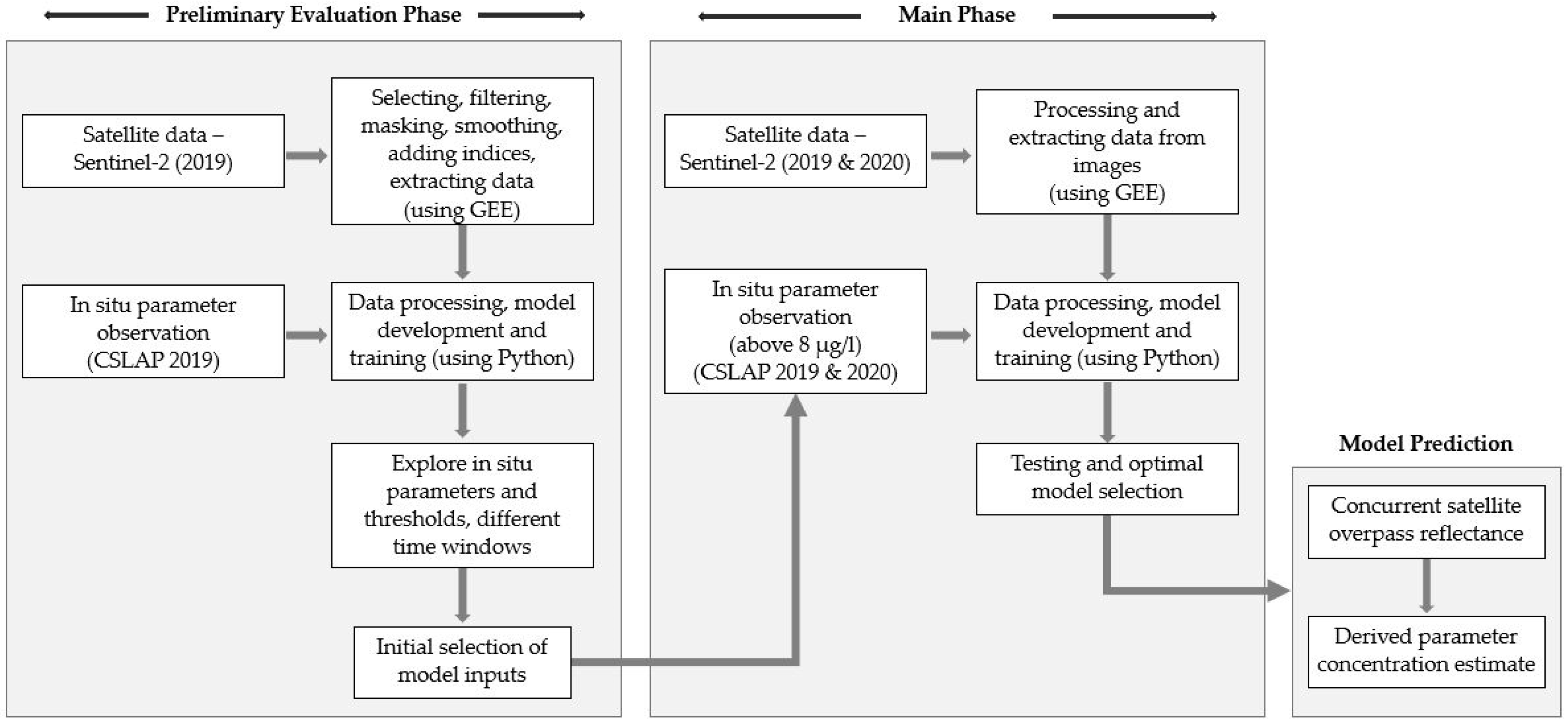
We used a phased approach to develop the empirical models in this study (Figure 2). We used empirical linear regression models to characterize the relationship between in situ observations of Chl-a and phycocyanin and image-based indices, developing models in Python 3.8.8 using different libraries such as pandas, numpy, matplotlib, and scikit-learn within a Jupyter notebook 6.3.0. In a preliminary evaluative phase, we used CSLAP in situ data from 2019 to develop models based on all available data and assessed models using R2 (Equation (1)) to make an initial selection of the model inputs. In the main phase, we developed models using the CSLAP in situ data from 2019 to 2020 above 8 µg/L, after randomly dividing these in situ data into training (70%) and testing (30%) components.
We evaluated model fit in the second phase using R2, RMSE (Equation (2)), and bias (MBE; Equation (3)) based on the training dataset [24]. Having selected an optimal model, its predictive capability was explored and validated by applying the model to the testing dataset and calculating R2, RMSE, and bias.
R 2 = 1 i = 1 n ( y i ŷ i ) 2 i = 1 n ( y i y ¯ ) 2
R M S E = 1 n i = 1 n ( y i ŷ i ) 2
M B E = 1 n i = 1 n y i ŷ i
where y i is the ith observed value, ŷ i is the ith predicted value, y ¯ is the mean value of observed values, and n is the number of observations.
We also characterized the predictive capability of the models, using confidence and prediction intervals [62]. A prediction interval includes a wider range of values than a confidence interval and relates to individual points, whereas a confidence interval relates to the mean value. The goal was to select an optimal algorithm with a strong model fit, but also having narrow prediction and confidence intervals to provide greater confidence in the model application. Figure 2 shows a flowchart of the various steps in the development of a retrieval model.
The simplest empirical algorithm is expressed as a linear regression model [8]:
Prediction = a + b × SPindex
where a and b are model parameters, and SPindex is a spectral index defined by two or more spectral bands of satellite imagery. Parameters a and b are calibrated by regressing between in situ measurements and the spectral index (SPindex) calculated from pixels of the Sentinel-2 L2A images at the sample site locations. Preliminary analysis found low concentration in situ field measurements of Chl-a and phycocyanin led to poor fit when establishing a linear regression model. Hence, we tested using different in situ parameter thresholds when calibrating the model.
We tested the importance of the temporal alignment of datasets by merging the field and satellite data in two different ways. First, we used satellite data acquired on the same date as the field samples. Second, we expanded the available data by using satellite data acquired with a one- or two-day separation from the field data acquisition (e.g., a one-day time window includes the data acquired on the same day as the field sample as well as those acquired one day before or after the field data were acquired). For the concurrent data, we had 874 field–satellite pairs, of which 87 had values above 8 µg/L, with 27 pairs in the test dataset. For the one-day time window, the total number of data points was 1954, with 200 data points above 8 µg/L, and a test dataset of 60 data points.
We tested a range of indices for the model input, e.g., using two-band (red-edge and red bands), three-band (red and two red-edge bands), and the normalized difference chlorophyll index (NDCI) (Table 1). We also modified four indices initially derived for lower spatial resolution instruments, such as MODIS and MERIS, by selecting the closest bands in Sentinel-2 satellite (bottom four rows in Table 1). Table 1 shows that bands from blue (band 2), green (band 3), red (band 4), and red-edge (bands 5, 6 and 8A) wavelengths are particularly important within the indices used as model input.
We assessed the accuracy of the optimal retrieval model using contingency tables for predictions based on both training and testing datasets. Additionally, as noted above, we also reported the confidence and prediction intervals [62] to validate the application of the best linear regression model using the randomly sampled testing dataset.
To enhance the results and assess the impact of different cloud mitigation approaches, we reanalyzed select models utilizing the Cloud Score+ S2 Harmonized V1 dataset in GEE. This dataset includes two QA bands that score on a continuous scale between 0 and 1, where values closer to 1 are considered clearer observations [58]. We tested different Cloud Score+ thresholds using CSLAP 2019 data, selected the most effective threshold to apply to the Sentinel-2 L2A data based on the best model fit, and then evaluated the performance of the best estimation model using the CSLAP 2019 and 2020 testing data. We applied thresholds of 30%, 40%, 50%, and 60% to the Cloud Score+ cs band. The cs band indicates how closely a pixel matches what we would expect from an ideal clear reference [58].

4. Results

4.1. Preliminary Phase

In the preliminary phase of the project, we utilized the 2019 CSLAP data to explore different in situ parameters and their thresholds, varying time windows (concurrent, one-day, and two-day time windows), and the impact of several lake characteristics (the trophic states of lakes, ecoregions in which lakes are located, dominant land cover in the surrounding watershed, and month of data collection) on model results.

4.1.1. Comparison of In Situ Parameter Thresholds

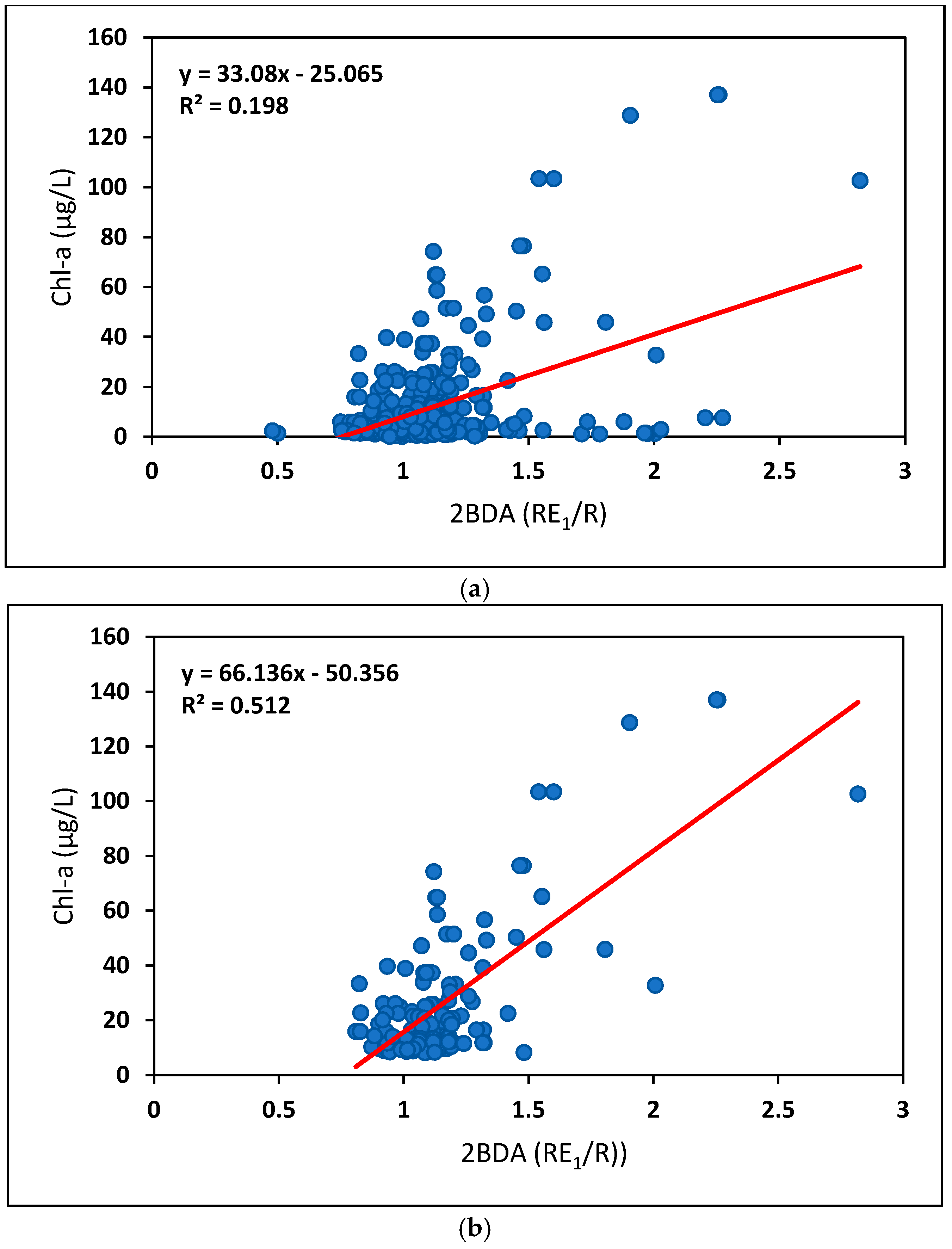
We developed linear regression models to relate in situ observations to Sentinel-2 indices. Our initial models showed weak R2 values when we included all available data regardless of the parameter used, e.g., Figure 3a illustrates the scatterplot (R2 < 0.2) for the model using the relationship between Chl-a and the two-band ratio (2BDA) built from red-edge and red data. We experimented with different thresholds and found that model fit improved when we limited in situ observations of Chl-a to the points above 8 μg/L, which aligns with the trophic index used by NYSDEC for eutrophic lakes [60]. Figure 3b shows the improvement in the 2BDA model fit by focusing on Chl-a points above 8 μg/L (R2 > 0.5). We found this threshold improved the model fit regardless of the index used for Chl-a models and we also achieved similar improvement in the phycocyanin models when these were also limited to field points with observations above 8 μg/L. We used this threshold for all subsequent analyses.
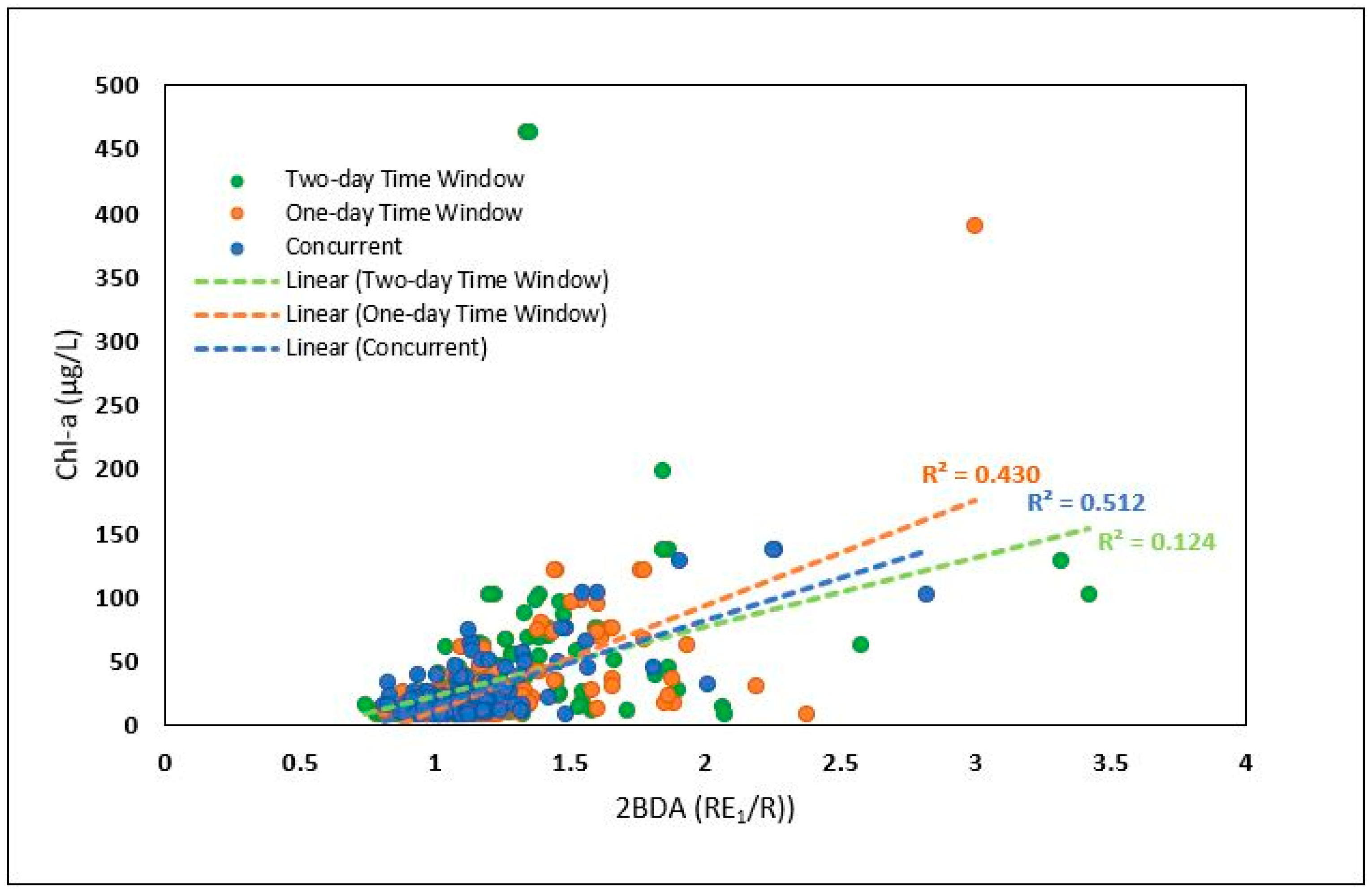
We used Sentinel-2 data acquired on the date of the in situ sampling as well as one and two days before and after the in situ sampling to consider the effect this time separation may have on the correlation between in situ and satellite data. This analysis was conducted using 2019 data and aimed to determine if an expanded time window could be used to mitigate any potential insufficiency in the number of concurrent data matches. Figure 4 shows the change in R2 with expansion of the time window, using the 2BDA-Chl-a model as an example. The best model was the concurrent data collection, but using a one-day time window had a relatively small reduction in R2 (from 0.51 to 0.45) and provided a substantially larger dataset. The models developed by expanding the time window out to two days resulted in an R2 of 0.24. This trend in model fit (similar results for concurrent and the one-day window with weaker results for the two-day window) held true for the different indices; hence, we excluded the two-day window from subsequent analyses.

4.1.2. Comparing Different Types of In Situ Measurements

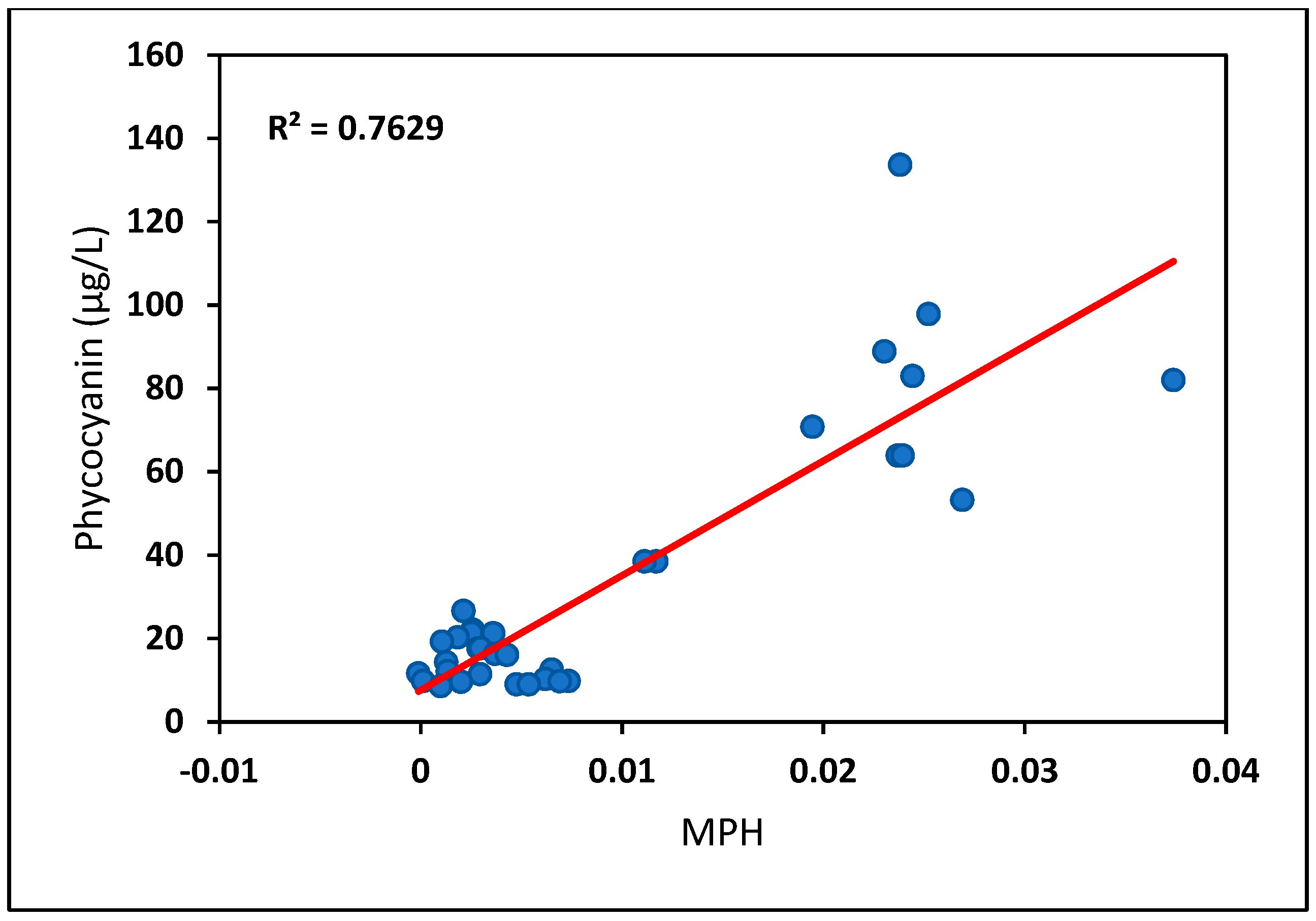
We compared models for Chl-a and phycocyanin, the two most commonly modeled phytoplankton pigments. Based on the finding that Chl-a models improved when data were limited to points above the eutrophic threshold (8 μg/L), we evaluated whether applying a similar detection threshold approach to the phycocyanin dataset was also beneficial to improve model fit. Empirical models improved using phycocyanin concentrations above 8 μg/L (R2 of 0.76) compared to those including all phycocyanin observations (R2 of 0.35). Because of this, and in the absence of a widely accepted limnology-based low-phycocyanin threshold, the 8 μg/L threshold was applied to phycocyanin.
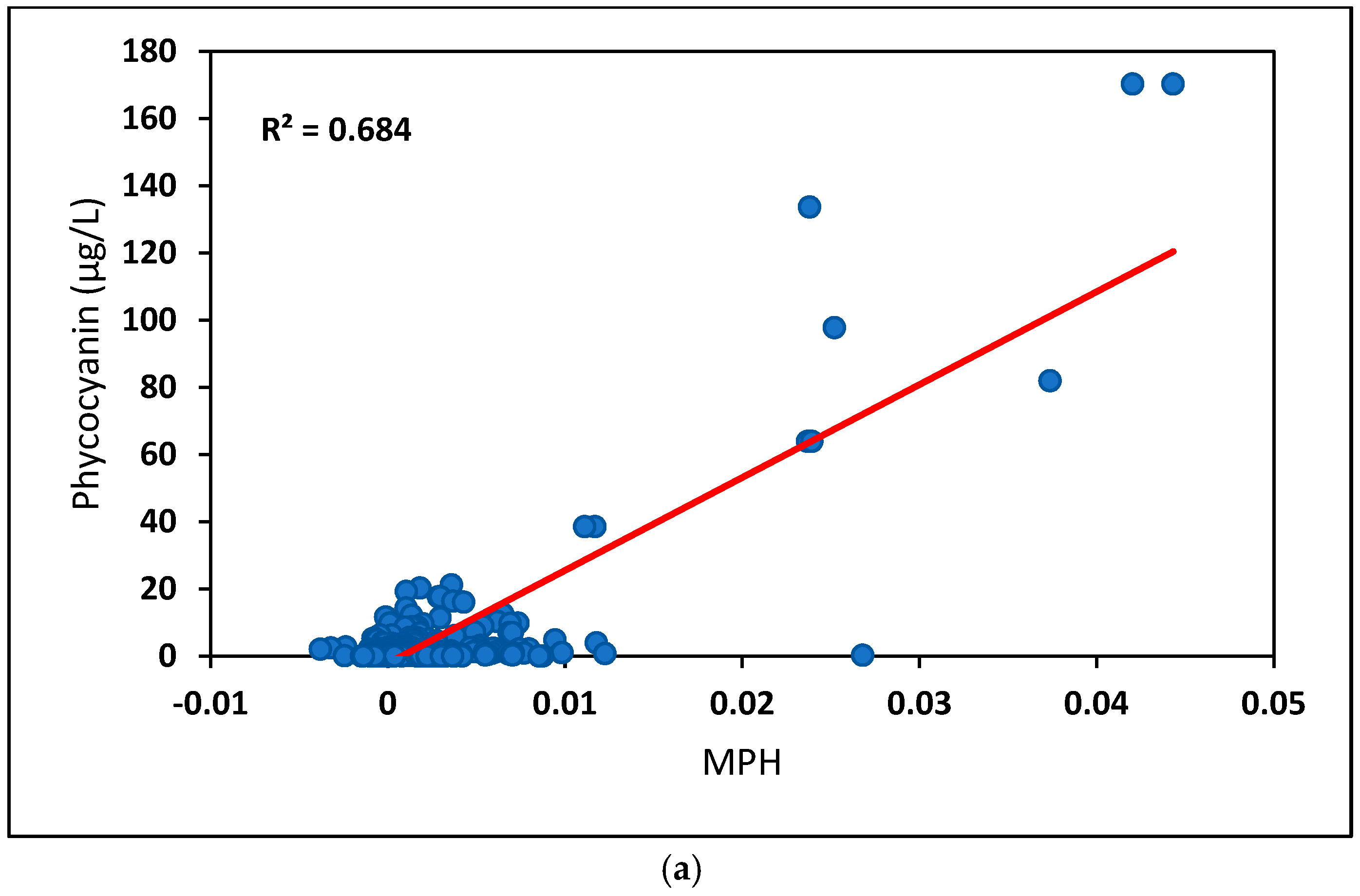
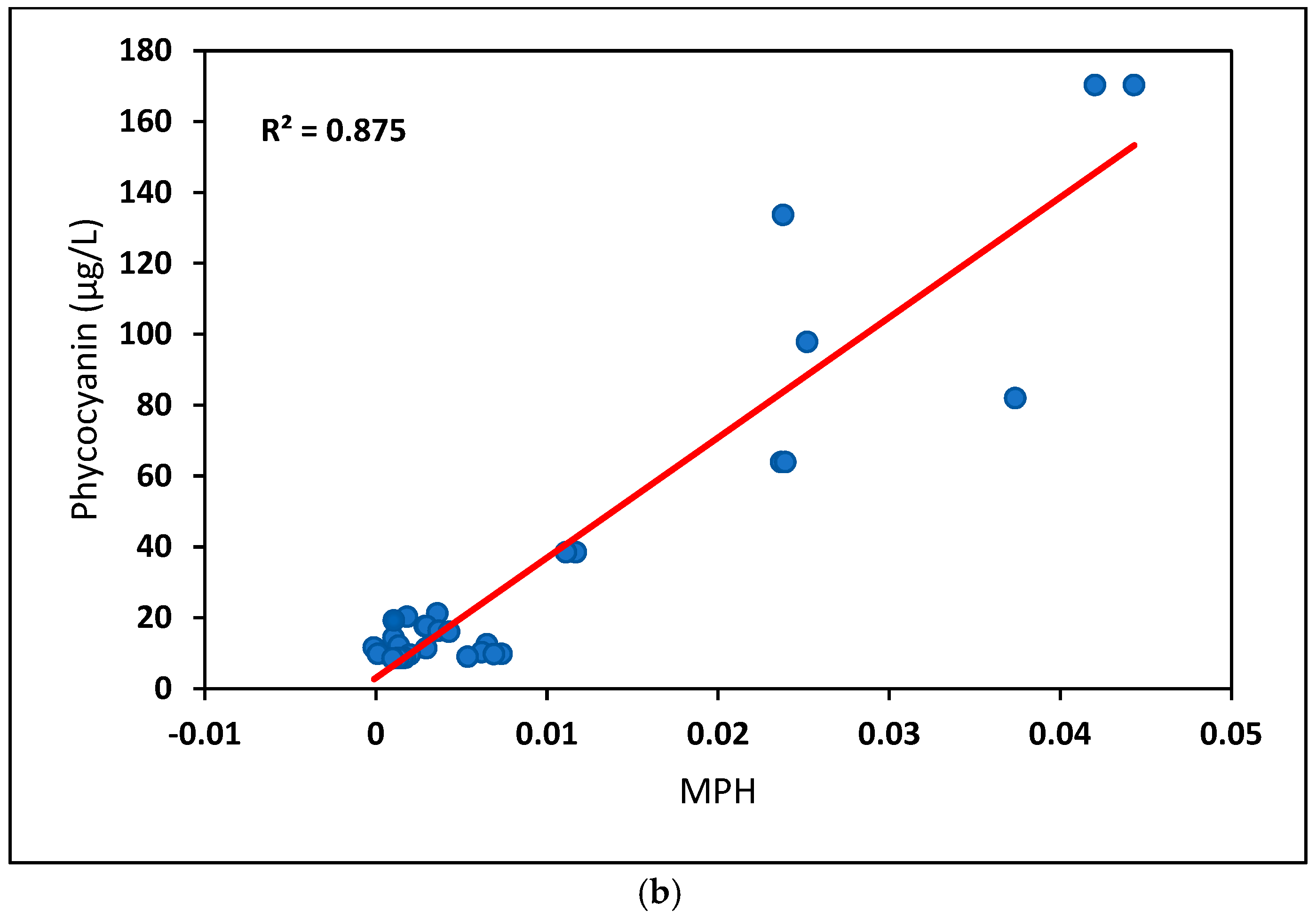
Figure 5 shows a scatterplot of the Sentinel-2 index and in situ phycocyanin concentrations above 8 μg/L. This scatterplot was based on the training data and shows the best model for phycocyanin in this preliminary phase. The highest R2 value for phycocyanin concentrations (0.76) was achieved when using MPH values. As shown in Figure 3b, the R2 value for Chl-a was distinctly lower, with the best model based on training data being the 2BDA model (0.51). Despite the lower R2 value for Chl-a, we continued to work with the data because of the importance of Chl-a estimation to lake managers.

4.1.3. Lake Characteristics

We also explored different lake characteristics that might influence model fit and classified the data based on several lake and regional characteristics. We classified data using the trophic states of lakes, ecoregions in which lakes are located, dominant land cover in the surrounding watershed, and month of data collection. We then used these classifications to determine if they impacted the fit of the regression model between in situ measurements and indices extracted from satellite data. Preliminary results showed that classification based on different lake characteristics or monthly classes individually did not improve the initial linear regression model results.

4.2. Main Phase

In the main phase of the project, we utilized the 2019 and 2020 CSLAP data randomly divided into training and testing datasets to assess the application of different retrieval models in estimating parameter concentration.

4.2.1. Comparison of Different Sentinel-2 Indices: Model Fit

Having tested various indices for Chl-a modeling during the preliminary phase, Table 2 summarizes the R2, RMSE, and MBE for linear regression models with seven indices for prediction of phycocyanin based on the testing dataset and contrasts this with the best Chl-a model. For both concurrent and one-day windows, the MPH model had the highest R2 and lowest RMSE, although the MBE magnitude for the two-band ratio model was slightly lower than other indices. The SABI model had the worst values across all metrics. Based on the sign of the reported MBE values, Table 2 also shows that for the concurrent data MPH and NDCI overestimate phycocyanin concentrations, while the other indices underestimated concentrations. Using the one-day window, all models underestimated phycocyanin concentrations. The R2 for the one-day time window tended to be similar to (or in some cases higher than) that for the concurrent data. The RMSE improved when moving to the one-day time window; conversely the magnitude of the MBE increased. The improvement in the model fit for the CI and MPH models is likely associated with the increase in data points available when the time window was expanded. This suggests that we can use a one-day time window between in situ and satellite data collection to expand our dataset without decreasing model fit.

4.2.2. Assessment of Model Prediction Accuracy

The indices that led to the best model fit of Chl-a and phycocyanin concentrations used the linear equations shown in Table 3. These models were analyzed to evaluate prediction accuracy of field observations known to have concentrations above 8 µg/L using Sentinel-2 data filtered by the QA60 bitmask using both concurrent data and a one-day time window.
Table 4 summarizes the contingency tables when the models shown in Table 3 were applied to the testing dataset. In this table, we categorized the field and predicted data as high (>24 μg/L), moderate (8–24 μg/L), and low (<8 μg/L), noting that these are not intended as regulatory guidelines. There are no consistent thresholds for such classification in the literature, but the 8 μg/L and 24 μg/L levels for Chl-a were selected based on trophic state and a common HAB alert level, respectively. As noted previously, the same thresholds were applied to phycocyanin for consistency. We note that the model training excluded in situ points below 8 μg/L; hence, the accuracy assessment using the training and testing data can only evaluate the accuracy of field points with ‘moderate’ and ‘high’ phycocyanin reports.
The results shown in Table 4 demonstrate that using concurrent models 70% and 65% of the predicted Chl-a values are correctly categorized as moderate and high, respectively, and 70% and 86% of the phycocyanin prediction values are correctly categorized as moderate and high, respectively. Using a one-day time window prediction model, the accuracy of moderate and high levels of Chl-a values were 74% and 71%, respectively, and for phycocyanin concentrations the levels were 83% and 96%, respectively.
Our primary goal in this evaluation was confirming that we did not have false negatives reported, i.e., field points that were known to have Chl-a or phycocyanin above 8 μg/L predicted by the remote sensing-based method as having low concentration. We note that one point in the concurrent dataset and three in a one-day dataset predicted low phycocyanin concentrations while the field phycocyanin concentrations were moderate or high (above 8 μg/L). After viewing the Sentinel-2 images for the four erroneous data points, we found that the errors were largely due to cloud contamination, which suggests that there may be issues with using the QA60 bitmask approach.

4.2.3. Confidence Interval for Test and Predicted Values of Phycocyanin

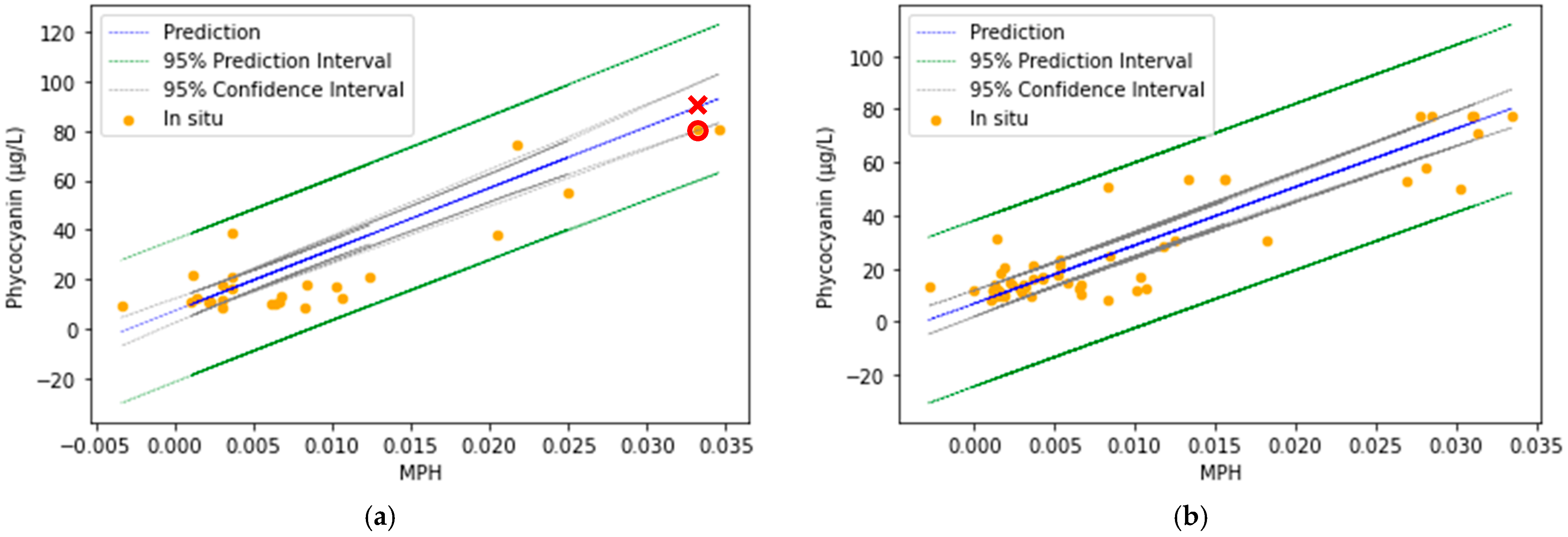
To illustrate a method for quantifying the confidence of our model results, we also used the randomly sampled testing dataset (CSLAP data with phycocyanin concentrations above 8 μg/L) to validate the MPH linear regression model for phycocyanin estimation from satellite data by determining the prediction and confidence intervals. Figure 6 shows the predicted and in situ values of phycocyanin, as well as the prediction and confidence intervals with a 0.05 level of significance (95% confidence) for the MPH model based on (a) concurrent data and (b) data with a one-day time window. One observation was removed from the analysis when visual interpretation confirmed that cloud contamination produced an outlier that was outside the feasible prediction range. The lower and upper lines of the prediction interval shown in Figure 6 mean that we are 95% sure that the predicted value for phycocyanin falls in this range, while the confidence interval limits say that we are 95% sure that average phycocyanin concentrations are within that range. As an example, in Figure 6a, for a selected location with an in situ phycocyanin observation of 80.91 μg/L (highlighted with a red circle), the Sentinel-2-based MPH value of 0.033 corresponds to a predicted phycocyanin concentration of 89.78 μg/L (marked with a red cross). By extending vertical lines from the cross in Figure 6, the corresponding prediction interval range demonstrates that we are 95% confident that the phycocyanin concentration for that point is in the range (59.88, 119.68 μg/L).

4.3. Alternate Cloud Mask Evaluation

4.3.1. Testing Cloud Score+ Thresholds

Similar to the preliminary phase described above, we used the CSLAP 2019 dataset to explore Cloud Score+ thresholds. As an example, Table 5 summarizes R2 for the MPH model based on different Cloud Score+ thresholds for phycocyanin concentration. Based on the results shown in Table 5, the most effective threshold appears to be 50%. Applying lower thresholds (30% or 40%) decreased the R2 of the model while applying higher thresholds (60%) decreased the available data as well as the R2 of the model.
Figure 7 illustrates the scatterplots for the correlation between in situ and Sentinel-2 data with the application of the 50% Cloud Score+ threshold for cloud masking. The application of Cloud Score+ for cloud masking improved the R2 values for the correlation between in situ and Sentinel-2 data. Based on the training dataset, the phycocyanin MPH model using the Cloud Score+ approach achieved an R2 value of 0.87, whereas the corresponding MPH model using the QA60 bitmask approach had an R2 value of 0.76.

4.3.2. Applying Cloud Score+ to 2019 and 2020 Data

Table 6 summarizes the R2, RMSE, and MBE for both Chl-a and phycocyanin models with concurrent and one-day time window data from the testing dataset. Models with concurrent data had better results for both Chl-a and phycocyanin. Using Cloud Score+ instead of the QA60 bitmask approach for phycocyanin improved the R2 (from 0.63 to 0.84) and reduced the RMSE (from 27 μg/L to 14.9 μg/L), but the MBE magnitude increased from 0.34 to -3.39. For Chl-a, while the R2 slightly improved (from 0.43 to 0.47), both the RMSE and MBE increased compared to the QA60 bitmask. Both the concurrent MPH model for phycocyanin and the 2BDA model for Chl-a overestimated prediction values when using the QA60 bitmask for cloud mitigation, and underestimated when using Cloud Score+. Unlike the previous findings, expanding the dataset using a one-day time window did not improve results when using Cloud Score+, with the R2 decreasing and the RMSE increasing. The MBE decreased for both Chl-a and phycocyanin estimation when expanding to the one-day window, with the models underestimating concentrations of both parameters.
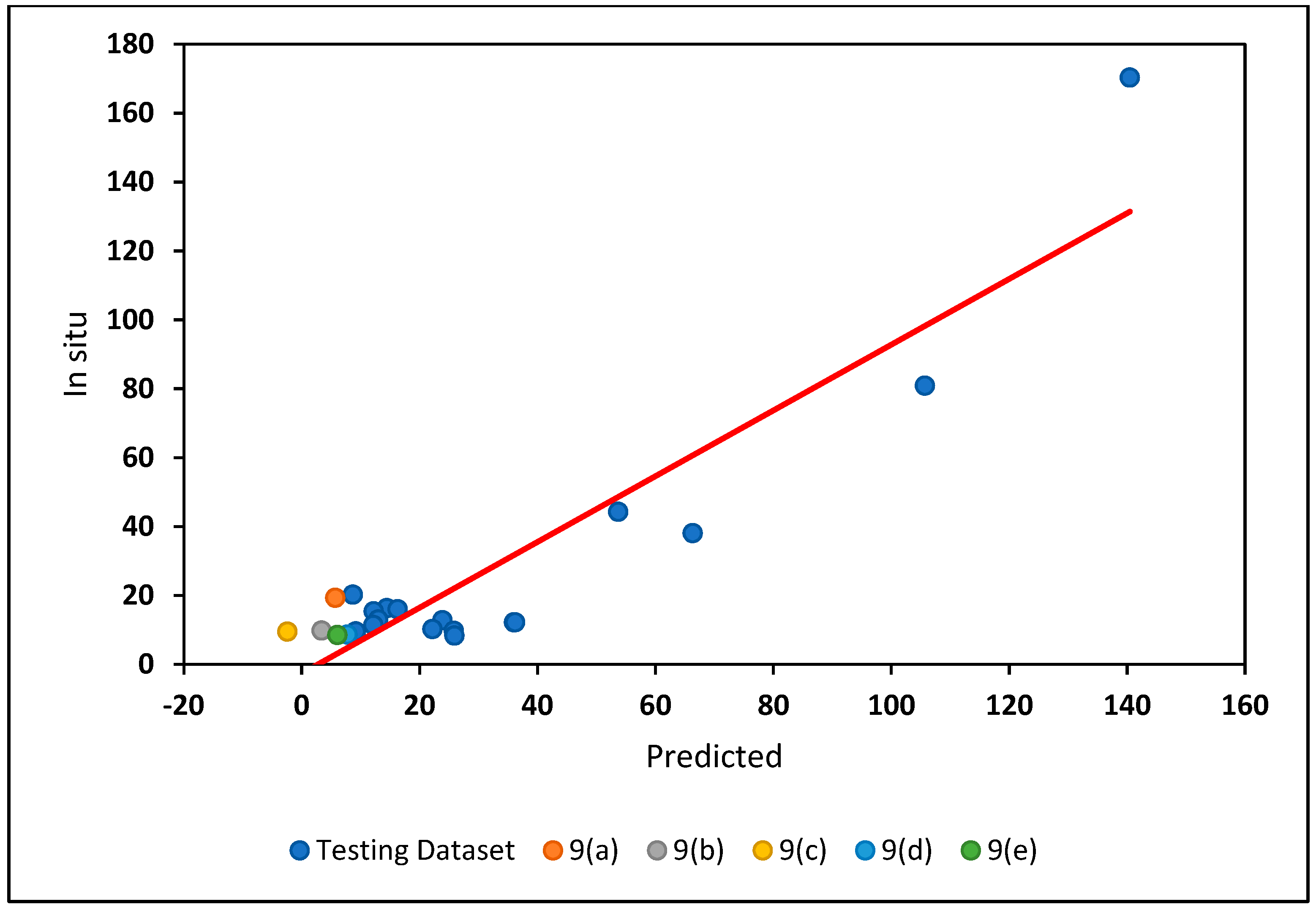
Figure 8 shows a scatterplot of in situ measurements vs. predicted values for the phycocyanin MPH model based on the concurrent testing dataset (CSLAP data for 2019 and 2020).
The indices that led to the best model fit of Chl-a and phycocyanin concentrations with the Cloud Score+ approach used the linear equations shown in Table 7. These models were analyzed to evaluate the prediction accuracy of field observations known to have concentrations above 8 µg/L using Sentinel-2 data filtered by the Cloud Score+ method.
The analysis of prediction accuracy focused on this model. Table 8 presents the contingency tables for the testing datasets, categorizing the field and predicted data as high (>24 μg/L), moderate (8–24 μg/L), or low (<8 μg/L), noting as above that the model training excluded in situ points below 8 μg/L. The results shown in Table 8 demonstrate that in the concurrent model, 56% and 69% of the predicted Chl-a values are correctly categorized as moderate and high, respectively, and 50% and 100% of the predicted phycocyanin values are correctly categorized as moderate and high, respectively. Using a one-day time window prediction model, the accuracies of the moderate and high levels of Chl-a concentrations were 71% and 73%, respectively, while the accuracies of the moderate and high levels of phycocyanin concentrations were 54% and 95%, respectively.
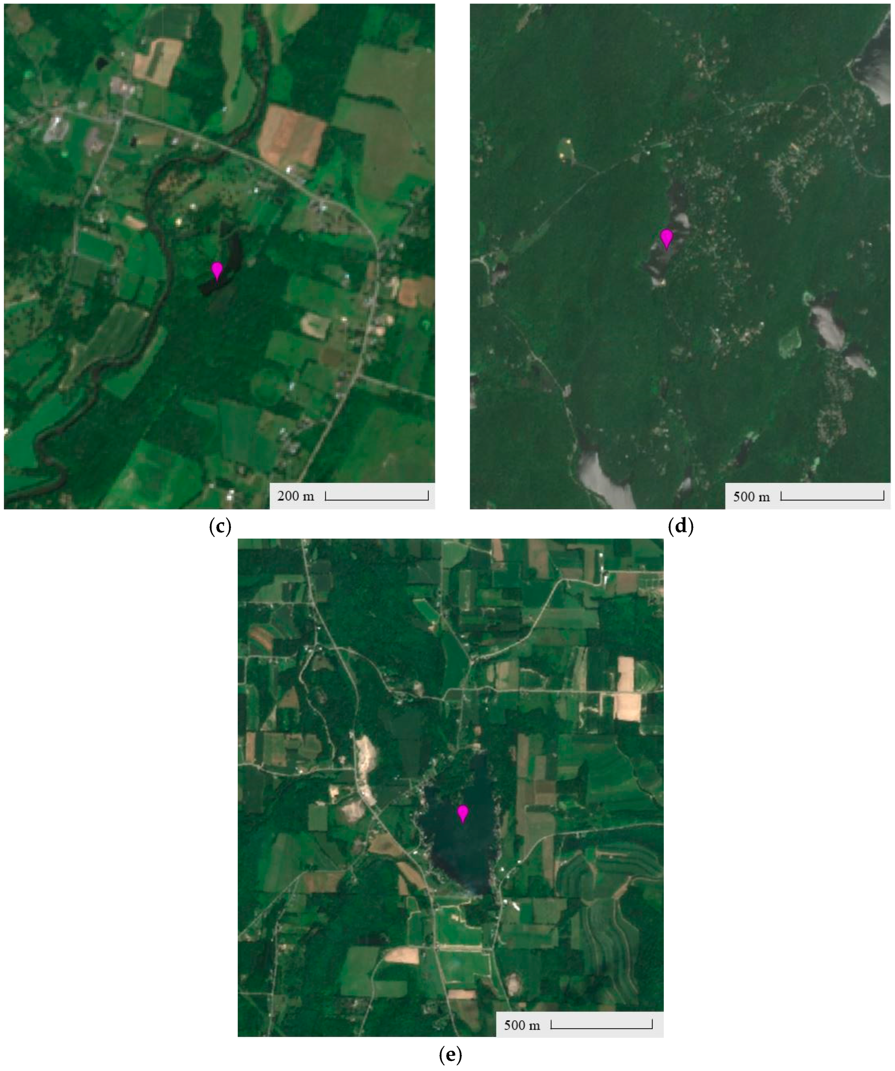
Figure 9 shows Sentinel-2 images corresponding to the five points in the concurrent testing data that were erroneously labeled as having low phycocyanin concentrations: one point with phycocyanin concentration of 19.3 μg/L (Figure 9a; area 4.066 km2) and four with field values near the 8 μg/L threshold (8.5–9.8 μg/L). The lakes shown in Figure 9b (area 0.673 km2) and Figure 9d (area 0.031 km2) illustrate scenarios where the errors are likely still due to cloud contamination or sun-glint. Figure 9c (area 0.189 km2) and Figure 9e (area 0.673 km2) depicted small lakes located in vegetation-covered areas, potentially with a mixed pixel response contributing to errors in those points. The reason for the error in Figure 9a is unclear: no cloud coverage was observed, and the lake is larger than the others.

5. Discussion

The primary objective of this study was to develop a model for estimating and monitoring Chl-a and phycocyanin concentrations across NYS lakes. After encountering early challenges related to the inaccuracy in estimating parameters with low concentrations, we implemented a threshold based on the trophic index utilized by NYSDEC for eutrophic lakes [60], restricting the model to in situ Chl-a and phycocyanin data above 8 μg/L. While studies commonly model Chl-a (e.g., [8,9,51,69,70]), our training analysis demonstrated a stronger correlation between satellite data and phycocyanin concentrations, and we found the phycocyanin model fit also improved when in situ data below 8 μg/L were excluded, likely because below 8 µg/L there is insufficient pigment in the water to give a clear spectral response. Other studies have also found it advantageous to apply thresholds on field data when modeling water quality. Soomets et al. [21] classified inland and coastal waters in the boreal region into five optical water types (OWTs)—clear, moderate, turbid, very turbid, and brown—and identified the best model for each class separately. Maciel et al. [71] employed two different thresholds on field data based on recommendations for cyanobacteria-dominant recreational water. They used 10 μg/L and 24 μg/L as the thresholds for low-risk and alert levels in recreational waters, respectively. They did not report statistics, but rather divided the initial dataset in different ways to visually determine the best estimation models for each subset. Zhao et al. [70] utilized OWTs to classify lakes into 13 classes and applied different retrieval models for each class. In this study, we considered data points above and below the established threshold; however, there was no specific trend for field points below 8 μg/L, hence we directed our focus towards field points above 8 μg/L.
We used Chl-a and phycocyanin concentrations above the 8 μg/L threshold as we tested a variety of model inputs. Initially, we examined two- and three-band ratios utilizing red and red-edge bands before applying four indices—CI [65], MCI [66], MPH [67], and SABI [68]—that were developed for lower spatial resolution instruments like MODIS and MERIS. Researchers have found that there are advantages in using the spectral strengths of these indices while utilizing the higher spatial resolution of Sentinel-2’s MSI sensor. For example, Maciel et al. [72] applied CI to estimate Chl-a levels in an estuary with highly variable turbidity using Sentinel-2 data, and Zhao et al. [70] employed MCI to assess Chl-a concentration using Sentinel-2 data. However, to the best of our knowledge, MPH application with Sentinel-2 data has not been reported in the literature. Matthews et al. [67] introduced the MPH algorithm for Chl-a estimation using a baseline subtraction technique to determine the switchable dominant peak’s height across the red and NIR bands of the MERIS. This peak is mainly attributed to sun-induced chlorophyll fluorescence and particulate backscatter and corresponds to the MERIS bands at 681, 709, or 753 nm. Matthews et al. [67] considered three different scenarios for HAB-affected waters: (1) low-medium biomass (Chl-a < 30 μg/L), where Chl-a concentrations are highly correlated with the red peak at 681 nm; (2) high biomass (Chl-a > 30 μg/L), where the red peak shifts to a longer wavelength and there is a strong correlation between Chl-a and the peak at 709 nm; and (3) extremely high biomass (Chl-a > 500 μg/L), where the red peak shifts to 750 nm. The CSLAP field data placed NYS lakes in the first two scenarios. However, as there is no Sentinel-2 band at 681 nm, we centered the MPH index at MSI band 5 (705 nm), capturing the second peak, with the baseline between band 4 (665 nm) and band 8A (865 nm). Moving to centering at the slightly higher wavelength may explain why the models relating in situ observations to the MPH values had better fit when values below 8 μg/L were excluded. These results are comparable to Matthews et al. [67], who applied the MERIS-based MPH model in waterbodies across different ranges of eutrophication levels (0.5 μg/L < Chl-a < 30 μg/L: R2 = 0.71, RMSE = 3.5 μg/L, n=36; Chl-a > 30 μg/L: R2 = 0.58 and RMSE = 46.6 μg/L). Unfortunately, while MERIS has excellent spectral characteristics, the spatial resolution (300 m at nadir) is unsuitable for small- and medium-sized lakes.
Despite the relatively high temporal resolution of the two-satellite Sentinel-2 constellation, the timing of in situ sampling did not always align with the overpass time of image acquisition, leading to a low number of concurrent ground and image points. We considered the application of one- and two-day time windows rather than only using concurrent in situ and remotely sensed data to help mitigate any data insufficiencies for model calibration and validation. While our results were poor when we expanded to the two-day window, we do not have sufficient evidence to recommend concurrent vs. a one-day time window, given the contradictory improvements in R2 versus the worsening in MBE. This may be due to the sensitivity of the MBE to outliers in the data introduced when considering a one-day delay. Kayastha et al. [69] applied different time windows for Chl-a modeling in ten reservoirs in Oklahoma, USA. They found models using a five-day time window had strong correlations between field and Sentinel-2 data. This was quite different from our findings that indicate that while a one-day time window may be applied, a two-day time window did not appear appropriate. Kayastha et al. [69] noted that their conclusions in terms of temporal matching may only be appropriate for man-made reservoirs and the difference here may relate to greater surface water movement in lakes exposed to winds vs. reservoirs in deeper, wind-protected valleys. Grendaitė and Petkevičius [73] also tested different time windows in applying Sentinel-2 data to estimating Chl-a in Baltic lakes and had strong model-fit when there was no more than a three-day time difference between in situ and satellite data. Their study used 1346 sample points, 44% of which had light to moderate algal blooms. Our study had a much smaller number of sample points and the increase in available data by expanding the time window may have led to better training of the one-day model, but the rapidly changing conditions may have limited further temporal expansion. These findings underscore the importance of dataset size in model performance and highlight the potential benefits of expanding the dataset when feasible, either through expanding the temporal match, but also through more intentionally aligning field-sampling schedules with the overpass time of Sentinel-2 imagery.
The results presented in Table 4 highlighted that when using imagery filtered using the QA60 bitmask approach, a portion of the testing prediction values were erroneously categorized as having low values, despite the corresponding in situ values being above 8 μg/L. Further examination of the corresponding Sentinel-2 images for the erroneous points identified cloud contamination as the key contributor to these errors. In response to the cloud-related challenges, we explored the potential of an alternate cloud masking approach, Cloud Score+ developed by Pasquarella et al. [58], to mitigate cloud contamination and enhance the accuracy of phycocyanin estimation. The selection of the optimal threshold is important in the Cloud Score+ cloud masking approach. Pasquarella et al. [58] initially proposed a threshold ranging between 50% and 65%. Cook et al. [74] filtered Sentinel-2 images with more than 80% cloud coverage and 10% snow coverage, and subsequently applied the Cloud Score+ algorithm using a 60% threshold. In a recent study, Gong et al. [53] compared a new cloud mitigation approach with four other methods, including Cloud Score+. Their proposed approach surpassed all other methods tested and may be worth exploring for future studies, though it increases complexity by using time-series data. Gong et al. [53] noted that while Cloud Score+ demonstrated improvement over existing techniques in masking unusable data like clouds and cloud shadows, it still necessitated manual adjustments to establish the optimal threshold and struggled to define the boundaries between clouds, thin clouds, and cloud shadows.
We tested various thresholds and found using our optimal Cloud Score+ threshold (50%) resulted in significant improvements in model fit compared to employing the QA60 bitmask approach. However, while model fit improved with the Cloud Score+ approach to cloud mitigation, our analysis (Table 8) still demonstrated prediction values in the testing datasets that were categorized as low, despite the corresponding in situ values exceeding 8 μg/L. In examining the corresponding Sentinel-2 L2A images we found cloudy points that led to erroneous predictions. The persistence of cloudy pixels even after applying the Cloud Score+ approach underscores the need for further examination of its application to inland waterbodies. Other errors may be attributed to the small size of the lakes and confusion through pixels mixing water with surrounding land cover. Additional exploration is needed to identify the exact source of error in cloud mitigation, which will be a key focus of our future work.
Previous studies (e.g., [75,76,77]), have highlighted the limitations of empirical models calibrated for specific locations and dates, emphasizing their lack of generalizability across different geographical areas and timeframes. In this study, we address these challenges by evaluating a diverse range of lakes within a broad spatial study area. Using GEE as a cloud computing platform, we developed a methodology for processing data at a large spatial scale. Our approach aimed to overcome the limitations of traditional approaches to training empirical models in specific waterbodies by using a large in situ dataset from a range of heterogeneous lakes. A recent study conducted by Zhao et al. [70] focused on estimating Chl-a on a broad scale by considering approximately 3000 of the largest global lakes (>50 km2). While their model demonstrated satisfactory performance modeling Chl-a concentration from Sentinel-2 data (R2 value of 0.74), the emphasis on large-sized lakes in their field data leaves the question of whether this is suitable for addressing the prevalence of high levels of algal blooms in many small- and mid-sized lakes worldwide unanswered. One of the significant findings of their study was the impact of meteorological factors and lake characteristics on Chl-a concentrations, which they incorporated using machine learning algorithms. This current study shows that our approach using an in situ dataset from a wide geographic and limnologic distribution of lakes can be successfully regressed against a Sentinel-2 dataset to achieve phycocyanin concentration estimates that are sufficiently accurate to be useful for practical purposes. Since the linear regression model is limited in terms of understanding interactions between different lake factors, in future studies, we will explore the potential benefits of applying alternative algorithms (e.g., machine learning approaches) that are capable of simultaneously incorporating multiple lake characteristics. This would enhance our understanding of the interactions between various lake factors, with the expectation that this could lead to more accurate model estimations.

6. Conclusions

This research marks an initial exploration into whether Sentinel-2-based empirical models can be employed as a tool to support the monitoring and assessing of water quality in small- and mid-size lakes (below ~200 km2) across New York State. By utilizing the Sentinel-2 L2A (surface reflectance) image collection in GEE and employing linear regression methods, we estimated the concentration of Chl-a and phycocyanin, which serve as key indicators of algal blooms. This approach can enable the identification of lakes with average values above a threshold of concern (e.g., the boundary between mesotrophic and eutrophic lakes at 8 µg/L, or HAB alert levels at 12, 24, 25, 30 µg/L or any other national level [78]) and holds promise for facilitating targeted field assessments, thereby supporting proactive measures for mitigating potential environmental impacts. In testing different in situ measurements, we found better model fit when field points were limited to observations above 8 μg/L. Of the variety of Sentinel-2 indices used as input to our linear regression models to correlate field-based observations with the Sentinel-2 L2A image collection in GEE, we had the greatest success with the MPH index when used with phycocyanin observations.
We explored two approaches for temporally matching in situ and satellite data points. Expanding the temporal window had the advantage of increasing the amount of data available for training the models. Model fit decreased substantially with the two-day window, but this was less problematic for the one-day time window. MBE increased for all models using data from the one-day time window vs. an exact temporal match, but R2 was often not negatively impacted. In fact, using the one-day window improved the R2 and RMSE for the MPH model in comparison to concurrent data, which is likely associated with the larger data volume available for training. Understanding the importance of temporally matching field and satellite data is critical to providing guidance, for example to CSLAP volunteers, about intentionally aligning field sampling schedules with satellite overpass dates.
To explore different approaches to mitigating the impact of clouds in Sentinel-2 images, we tested cloud masking using the ESA QA60 bitmask and the Cloud Score+ approaches. Our best model for estimating phycocyanin from Sentinel-2 images filtered by the QA60 bitmask cloud detection used the MPH index with an R2 of 0.63 for concurrent data and 0.71 for a one-day time window when tested on data not used in model calibration. Using Cloud Score+ cloud detection on the corresponding model resulted in an R2 of 0.84 for the concurrent data. These models had strong predictive power when tested on lakes that were known to have high phycocyanin concentrations, with very few false negatives, but only using field observations above 8 μg/L did not enable assessment of lakes with low phycocyanin levels; hence, the potential for false positives was not known. While erring on the side of minimizing false negatives seems appropriate, refining the model to also mitigate false positives will better focus resources. We used the randomly sampled testing dataset to validate the MPH linear regression model by determining the prediction and confidence intervals. This analysis is important to understand the confidence in the model output.
The results of this study provide a method for estimating Chl-a and phycocyanin concentrations to monitor small- and mid-sized heterogeneous lakes across a broad spatial area, to detect those at high risk of algal blooms. Such remote sensing-based methods are critical to maximize the efficiency of limited resources for field-based evaluation. While the model fit is weaker for Chl-a, an important component of the method presented is considering statistical measures to describe the model application and estimate uncertainty in model predictions. The confidence intervals recommended in this study ensure the image-derived output has a place in management decisions. Future studies will focus on applying alternative algorithms, such as machine learning approaches, to explore the effect of various lake characteristics on the performance of estimation models and expanding in situ data to enhance model training and achieve more accurate estimation models.

Author Contributions

Conceptualization, S.A.N., L.M. and L.J.Q.; methodology, S.A.N., L.J.Q. and L.M.; software, S.A.N.; validation, S.A.N.; formal analysis, S.A.N.; resources, L.M. and L.J.Q.; data curation, S.A.N.; writing—original draft preparation, S.A.N.; writing—review and editing, L.M., L.J.Q.; project administration, L.J.Q.; funding acquisition, L.M. and L.J.Q. All authors have read and agreed to the published version of the manuscript.

Funding

This study was primarily funded by NYSDEC with additional support from the U.S. Geological Survey under Grant/Cooperative Agreement No. G18AP00077 and G23AP00683.

Data Availability Statement

Harmonized Sentinel-2 L2A images and Cloud Score+ S2 Harmonized V1 data used in this study are available at Google Earth Engine (https://earthengine.google.com, accessed on 19 September 2024).

Acknowledgments

We would like to thank the Citizens Statewide Lake Assessment Program (CSLAP) citizen scientists for collecting and providing the in situ data used in this study. We thank the European Space Agency (ESA) for providing Sentinel-2 data.

Conflicts of Interest

The authors declare no conflict of interest.

References

  1. Ho, J.C.; Michalak, A.M.; Pahlevan, N. Widespread global increase in intense lake phytoplankton blooms since the 1980s. Nature 2019, 574, 667–670. [Google Scholar] [CrossRef]
  2. Otten, T.G.; Paerl, H.W. Health effects of toxic cyanobacteria in U.S. drinking and recreational waters: Our current understanding and proposed direction. Curr. Environ. Health Rep. 2015, 2, 75–84. [Google Scholar] [CrossRef] [PubMed]
  3. Michalak, A.M.; Anderson, E.J.; Beletsky, D.; Boland, S.; Bosch, N.S.; Bridgeman, T.B.; Chaffin, J.D.; Cho, K.; Confesor, R.; Daloğlu, I.; et al. Record-setting algal bloom in Lake Erie caused by agricultural and meteorological trends consistent with expected future conditions. Proc. Natl. Acad. Sci. USA 2013, 110, 6448–6452. [Google Scholar] [CrossRef] [PubMed]
  4. Gorney, R.M.; June, S.G.; Stainbrook, K.M.; Smith, A.J. Detections of cyanobacteria harmful algal blooms (cyanoHABs) in New York State, United States (2012–2020). Lake Reserv. Manag. 2023, 39, 21–36. [Google Scholar] [CrossRef]
  5. Moses, W.J.; Gitelson, A.A.; Berdnikov, S.; Povazhny, V. Estimation of chlorophyll-a concentration in case II waters using MODIS and MERIS data—Successes and challenges. Environ. Res. Lett. 2009, 4, 045005. [Google Scholar] [CrossRef]
  6. Zhang, Y.; Ma, R.; Duan, H.; Loiselle, S.; Xu, J. A spectral decomposition algorithm for estimating chlorophyll-a concentrations in Lake Taihu, China. Remote Sens. 2014, 6, 5090–5106. [Google Scholar] [CrossRef]
  7. Kutser, T.; Paavel, B.; Verpoorter, C.; Ligi, M.; Soomets, T.; Toming, K.; Casal, G. Remote sensing of black lakes and using 810 nm reflectance peak for retrieving water quality parameters of optically complex waters. Remote Sens. 2016, 8, 497. [Google Scholar] [CrossRef]
  8. Xu, M.; Liu, H.; Beck, R.; Lekki, J.; Yang, B.; Shu, S.; Liu, Y.; Benko, T.; Anderson, R.; Tokars, R.; et al. Regionally and locally adaptive models for retrieving chlorophyll-a concentration in inland waters from remotely sensed multispectral and hyperspectral imagery. IEEE Trans. Geosci. Remote Sens. 2019, 57, 4758–4774. [Google Scholar] [CrossRef]
  9. Ansper, A.; Alikas, K. Retrieval of chlorophyll a from Sentinel-2 MSI data for the European Union Water framework directive reporting purposes. Remote Sens. 2019, 11, 64. [Google Scholar] [CrossRef]
  10. Yentsch, C.S. The influence of phytoplankton pigments on the colour of seawater. Deep Sea Res. 1960, 7, 1–9. [Google Scholar] [CrossRef]
  11. Clark, G.L.; Ewing, G.C.; Lorenzen, C.J. Spectra of backscattered light from the sea obtained from aircraft as a measure of chlorophyll concentration. Science 1970, 167, 1119–1121. [Google Scholar] [CrossRef] [PubMed]
  12. Hovis, W.A. The Nimbus-7 Coastal Zone Color Scanner (CZCS) Program. In Oceanography from Space; Gower, J.F.R., Ed.; Springer: Boston, MA, USA, 1981; Volume 13. [Google Scholar] [CrossRef]
  13. Clark, D.W. Phytoplankton pigment algorithms for the Nimbus-7 CZCS. In Oceanography from Space; Gower, J.F.R., Ed.; Plenum: New York, NY, USA, 1981; pp. 227–237In. [Google Scholar] [CrossRef]
  14. O’Reilly, J.E.; Maritorena, S.; Mitchell, G.; Siegel, D.A.; Carder, K.L.; Garver, S.A.; Kahru, M.; McClain, C. Ocean color chlorophyll algorithms for SeaWiFS. J. Geophys. Res. 1998, 103, 24937–24953. [Google Scholar] [CrossRef]
  15. Esaias, W.E.; Abbot, M.R.; Barton, I.J.; Brown, O.B.; Campbell, J.W.; Carder, K.L.; Clark, D.K.; Evans, R.H.; Hoge, F.E.; Gordon, H.R.; et al. An overview of MODIS capabilities for ocean science observations. IEEE Trans. Geosci. Remote Sens. 1998, 36, 1250–1265. [Google Scholar] [CrossRef]
  16. Gons, H.J.; Rijkeboer, M.; Ruddick, K.G. A chlorophyll-retrieval algorithm for satellite imagery (Medium Resolution Imaging Spectrometer) of inland and coastal waters. J. Plankton Res. 2002, 24, 947–951. [Google Scholar] [CrossRef]
  17. New York State Department of Environmental Conservation. Priority Waterbody List—Lakes 2024, Shapefile. Available online: https://data.gis.ny.gov/datasets/nysdec::priority-waterbody-list-lakes/explore (accessed on 1 August 2024).
  18. European Space Agency (ESA). Sentinel-2, The Operational Copernicus Optical High Resolution Land Mission; European Space Agency: Paris, France, 2013; Available online: http://esamultimedia.esa.int/docs/S2-Data_Sheet.pdf (accessed on 30 September 2019).
  19. Batur, E.; Maktav, D. Assessment of surface water quality by using satellite images fusion based on PCA method in the Lake Gala, Turkey. IEEE Trans. Geosci. Remote Sens. 2019, 57, 2983–2989. [Google Scholar] [CrossRef]
  20. Bresciani, M.; Cazzaniga, I.; Austoni, M.; Sforzi, T.; Buzzi, F.; Morabito, G.; Giardino, C. Mapping phytoplankton blooms in deep subalpine lakes from Sentinel-2A and Landsat-8. Hydrobiologia 2018, 824, 197–214. [Google Scholar] [CrossRef]
  21. Soomets, T.; Uudeberg, K.; Jakovels, D.; Brauns, A.; Zagars, M.; Kutser, T. Validation and comparison of water quality products in Baltic Lakes using Sentinel-2 MSI and Sentinel-3 OLCI data. Sensors 2020, 20, 742. [Google Scholar] [CrossRef]
  22. Ha, N.T.T.; Thao, N.T.P.K.; Katsuaki, N.; Mai, T.N. Selecting the Best Band Ratio to Estimate Chlorophyll-a Concentration in a Tropical Freshwater Lake Using Sentinel-2A Images from a Case Study of Lake Ba Be (Northern Vietnam). ISPRS Int. J. Geo-Inf. 2017, 6, 2220–9964. [Google Scholar] [CrossRef]
  23. Beck, R.; Xu, M.; Zhan, S.; Johansen, R.; Liu, H.; Tong, S.; Yang, B.; Shu, S.; Wu, Q.; Wang, S.; et al. Comparison of satellite reflectance algorithms for estimating turbidity and cyanobacterial concentrations in productive freshwaters using hyperspectral aircraft imagery and dense coincident surface observations. J. Great Lakes Res. 2019, 45, 413–433. [Google Scholar] [CrossRef]
  24. Chen, J.; Zhu, W.; Tian, Y.Q.; Yu, Q.; Zheng, Y.; Huang, L. Remote estimation of colored dissolved organic matter and chlorophyll-a in Lake Huron using Sentinel-2 measurements. J. Appl. Remote Sens. 2017, 11, 036007. [Google Scholar] [CrossRef]
  25. Ogashawara, I.; Kiel, C.; Jechow, A.; Kohnert, K.; Ruhtz, T.; Grossart, H.-P.; Hölker, F.; Nejstgaard, J.C.; Berger, S.A.; Wollrab, S. The use of Sentinel-2 for chlorophyll-a spatial dynamics assessment: A comparative study on different lakes in Northern Germany. Remote Sens. 2021, 13, 1542. [Google Scholar] [CrossRef]
  26. Mandanici, E.; Bitelli, G. Preliminary comparison of Sentinel-2 and Landsat 8 imagery for a combined use. Remote Sens. 2016, 8, 1014. [Google Scholar] [CrossRef]
  27. Bresciani, M.; Pinardi, M.; Free, G.; Luciani, G.; Ghebrehiwot, S.; Laanen, M.; Peters, S.; Della Bella, V.; Padula, R.; Giardino, C. The use of multisource optical sensors to study phytoplankton spatio-temporal variation in a shallow turbid lake. Water 2020, 12, 284. [Google Scholar] [CrossRef]
  28. Wang, M.; Yao, Y.; Shen, Q.; Gao, H.; Li, J.; Zhang, F.; Wu, Q. Time-series analysis of surface-water quality in Xiong’an new area, 2016–2019. J. Indian Soc. Remote Sens. 2021, 49, 857–872. [Google Scholar] [CrossRef]
  29. Cazzaniga, I.; Bresciani, M.; Colombo, R.; Della Bella, V.; Padula, R.; Giardino, C. A comparison of Sentinel-3-OLCI and Sentinel-2-MSI-derived Chlorophyll-a maps for two large Italian lakes. Remote Sens. Lett. 2019, 10, 978–987. [Google Scholar] [CrossRef]
  30. Giardino, C.; Candiani, G.; Bresciani, M.; Lee, Z.; Gagliano, S.; Pepe, M. BOMBER: A tool for estimating water quality and bottom properties from remote sensing images. Comput. Geosci. 2012, 45, 313–318. [Google Scholar] [CrossRef]
  31. Niroumand-Jadidi, M.; Bovolo, F.; Bruzzone, L. Water quality retrieval from PRISMA hyperspectral images: First experience in a turbid lake and comparison with Sentinel-2. Remote Sens. 2020, 12, 3984. [Google Scholar] [CrossRef]
  32. Pereira-Sandoval, M.; Ruescas, A.; Urrego, P.; Ruiz-Verdú, A.; Delegido, J.; Tenjo, C.; Soria-Perpinyà, X.; Vicente, E.; Soria, J.; Moreno, J. Evaluation of atmospheric correction algorithms over Spanish inland waters for Sentinel-2 multi spectral imagery data. Remote Sens. 2019, 11, 1469. [Google Scholar] [CrossRef]
  33. International Ocean-Colour Coordinating Group (IOCCG). Remote Sensing of Ocean Colour in Coastal, and Other Optically Complex, Waters; Sathyendranath, S., Ed.; Reports of the International Ocean-Colour Coordinating Group, No. 3; IOCCG: Dartmouth, MA, Canada, 2000. [Google Scholar] [CrossRef]
  34. Matthews, M.W. A current review of empirical procedures of remote sensing in Inland and near-coastal transitional waters. Int. J. Remote Sens. 2011, 32, 6855–6899. [Google Scholar] [CrossRef]
  35. Morel, A.; Prieur, L. Analysis of variations in ocean color. Limnol. Oceanogr. 1977, 22, 709–722. [Google Scholar] [CrossRef]
  36. Fell, F.; Fischer, E.; Schaale, M.; Schroder, T. Retrieval of chlorophyll concentration from MERIS measurements in the spectral range of the sun-induced chlorophyll fluorescence. Proc. SPIE 2003, 4892, 116–123. [Google Scholar] [CrossRef]
  37. Matthews, M.W.; Bernard, S.; Winter, K. Remote sensing of cyanobacteria-dominant algal blooms and water quality parameters in Zeekoevlei, a small hypertrophic lake, using MERIS. Remote Sens. Environ. 2010, 114, 2070–2087. [Google Scholar] [CrossRef]
  38. Lins, R.C.; Martinez, J.M.; Marques, D.D.; Cirilo, J.A.; Fragoso, C.R. Assessment of chlorophyll-a remote sensing algorithms in a productive tropical estuarine-lagoon system. Remote Sens. 2017, 9, 516. [Google Scholar] [CrossRef]
  39. Gitelson, A.A. The peak near 700 nm on radiance spectra of algae and water: Relationships of its magnitude and position with chlorophyll. Int. J. Remote Sens. 1992, 13, 3367–3373. [Google Scholar] [CrossRef]
  40. Gitelson, A.A.; Gritz, Y.; Merzlyak, M.N. Relationships between leaf chlorophyll content and spectral reflectance and algorithms for non-destructive chlorophyll assessment in higher plant leaves. J. Plant Physiol. 2003, 160, 271–282. [Google Scholar] [CrossRef]
  41. Le, C.; Li, Y.; Zha, Y.; Sun, D.; Huang, C.; Lu, H. A four-band semi-analytical model for estimating chlorophyll-a in highly turbid lakes: The case of Taihu Lake, China. Remote Sens. Environ. 2009, 113, 1175–1182. [Google Scholar] [CrossRef]
  42. Dekker, A.G. Detection of the Optical Water Quality Parameters for Eutrophic Waters by High Resolution Remote Sensing. Ph.D. Thesis, Free University, Amsterdam, The Netherlands, 1993. Available online: https://research.vu.nl/ws/portalfiles/portal/62846616/complete+dissertation.pdf (accessed on 23 August 2024).
  43. Schalles, J.F.; Yacobi, Y.Z. Remote detection and seasonal patterns of phycocyanin, carotenoid and chlorophyll pigments in eutrophic waters. Ergeb. Limnol. 2000, 55, 153–168. [Google Scholar]
  44. Simis, S.; Peters, S.; Gons, H. Remote sensing of the cyanobacterial pigment phycocyanin in turbid inland water. Limnol. Oceanogr. 2005, 50, 237–245. [Google Scholar] [CrossRef]
  45. Mishra, S.; Mishra, D.R.; Schluchter, W.M. A novel algorithm for predicting phycocyanin concentrations in cyanobacteria: A proximal hyperspectral remote sensing approach. Remote Sens. 2009, 1, 758–775. [Google Scholar] [CrossRef]
  46. Mishra, S.; Mishra, D.R. A novel remote sensing algorithm to quantify phycocyanin in cyanobacterial algal blooms. Environ. Res. Lett. 2014, 9, 114003. [Google Scholar] [CrossRef]
  47. Yan, Y.; Zhongjue, B.; Jingan, S. Phycocyanin concentration retrieval in inland waters: A comparative review of the remote sensing techniques and algorithms. J. Great Lakes Res. 2018, 44, 748–755. [Google Scholar] [CrossRef]
  48. Woźniak, M.; Bradtke, K.M.; Darecki, M.; Krężel, A. Empirical Model for Phycocyanin Concentration Estimation as an Indicator of Cyanobacterial Bloom in the Optically Complex Coastal Waters of the Baltic Sea. Remote Sens. 2016, 8, 212. [Google Scholar] [CrossRef]
  49. Sòria-Perpinyà, X.; Vicente, E.; Urrego, P.; Pereira-Sandoval, M.; Tenjo, C.; Ruíz-Verdú, A.; Delegido, J.; Soria, J.M.; Peña, R.; Moreno, J. Validation of Water Quality Monitoring Algorithms for Sentinel-2 and Sentinel-3 in Mediterranean Inland Waters with In Situ Reflectance Data. Water 2021, 13, 686. [Google Scholar] [CrossRef]
  50. Li, S.; Song, K.; Wang, S.; Liu, G.; Wen, Z.; Shang, Y.; Lyu, L.; Chen, F.; Xu, S.; Tao, H.; et al. Quantification of chlorophyll-a in typical lakes across China using Sentinel-2 MSI imagery with machine learning algorithm. Sci. Total Environ. 2021, 778, 146271. [Google Scholar] [CrossRef] [PubMed]
  51. Aptoula, E.; Ariman, S. Chlorophyll-a Retrieval from Sentinel-2 Images using convolutional neural network regression. IEEE Geosci. Remote Sens. Lett. 2021, 19, 6002605. [Google Scholar] [CrossRef]
  52. Yildiz, B.; Bilbao, J.I.; Sproul, A.B. A review and analysis of regression and machine learning models on commercial building electricity load forecasting. Renew. Sustain. Energy Rev. 2017, 73, 1104–1122. [Google Scholar] [CrossRef]
  53. Gong, C.; Yin, R.; Long, T.; Jiao, W.; He, G.; Wang, G. Spatial–Temporal Approach and Dataset for Enhancing Cloud Detection in Sentinel-2 Imagery: A Case Study in China. Remote Sens. 2024, 16, 973. [Google Scholar] [CrossRef]
  54. Main-Knorn, M.; Pflug, B.; Louis, J.; Debaecker, V.; Müller-Wilm, U.; Gascon, F. Sen2Cor for Sentinel-2. In Image and Signal Processing for Remote Sensing XXIII; SPIE: Bellingham, DC, USA, 2017; Volume 10427, pp. 37–48. [Google Scholar] [CrossRef]
  55. Coluzzi, R.; Imbrenda, V.; Lanfredi, M.; Simoniello, T. A first assessment of the Sentinel-2 Level 1-C cloud mask product to support informed surface analyses. Remote Sens. Environ. 2018, 217, 426–443. [Google Scholar] [CrossRef]
  56. Qiu, S.; Zhu, Z.; He, B. Fmask 4.0: Improved cloud and cloud shadow detection in Landsats 4–8 and Sentinel-2 imagery. Remote Sens. Environ. 2019, 231, 111205. [Google Scholar] [CrossRef]
  57. Zhang, H.; Huang, Q.; Zhai, H.; Zhang, L. Multi-temporal cloud detection based on robust PCA for optical remote sensing imagery. Comput. Electron. Agric. 2021, 188, 106342. [Google Scholar] [CrossRef]
  58. Pasquarella, V.J.; Brown, C.F.; Czerwinski, W.; Rucklidge, W.J. Comprehensive quality assessment of optical satellite imagery using weakly supervised video learning. In Proceedings of the IEEE/CVF Conference on Computer Vision and Pattern Recognition, Vancouver, BC, Canada, 17–24 June 2023; pp. 2124–2134. [Google Scholar]
  59. Prestigiacomo, A.R.; June, S.G.; Gorney, R.M.; Smith, A.J.; Clinkhammer, A.C. An evaluation of a spectral fluorometer for monitoring chlorophyll a in New York State Lakes. Lake Reserv. Manag. 2022, 38, 318–333. [Google Scholar] [CrossRef]
  60. Carlson, R.E. A trophic state index for lakes. Limnol. Oceanogr. 1977, 22, 361–369. [Google Scholar] [CrossRef]
  61. NYSDEC Standard Operating Procedure: Collection of Lake Water Quality Samples; Albany: New York, USA, 2021; p. 39. Available online: https://extapps.dec.ny.gov/docs/water_pdf/soplakesampling721.pdf (accessed on 1 August 2024).
  62. Heskes, T. Practical confidence and prediction intervals. In Advances in Neural Information Processing Systems; MIT Press: Cambridge, MA, USA, 1996; Volume 9. [Google Scholar]
  63. Zimba, P.V.; Gitelson, A. Remote estimation of chlorophyll concentration in hyper-eutrophic aquatic systems: Model tuning and accuracy optimization. Aquaculture 2006, 256, 272–286. [Google Scholar] [CrossRef]
  64. Mishra, S.; Mishra, D.R. Normalized difference chlorophyll index: A novel model for remote estimation of chlorophyll—A concentration in turbid productive waters. Remote Sens. Environ. 2012, 117, 394–406. [Google Scholar] [CrossRef]
  65. Wynne, T.T.; Stumpf, R.P.; Tomlinson, M.C.; Warner, R.A.; Tester, P.A.; Dyble, J.; Fahnenstiel, G.L. Relating spectral shape to cyanobacterial Blooms in the Laurentian Great Lakes. Int. J. Remote Sens. 2008, 29, 3665–3672. [Google Scholar] [CrossRef]
  66. Gower, J.; King, S.; Borstad, G.; Brown, L. Detection of intense plankton blooms using the 709 nm band of the MERIS imaging spectrometer. Int. J. Remote Sens. 2005, 26, 2005–2012. [Google Scholar] [CrossRef]
  67. Matthews, M.W.; Bernard, S.; Robertson, L. An algorithm for detecting trophic status (chlorophyll-a), cyanobacterial-dominance, surface scums and floating vegetation in inland and coastal waters. Remote Sens. Environ 2012, 124, 637–652. [Google Scholar] [CrossRef]
  68. Alawadi, F. Detection of Surface Algal Blooms Using the Newly Developed Algorithm Surface Algal Bloom Index (SABI); SPIE: Bellingham, DC, USA, 2010; Volume 7825, pp. 782506-1–782506-14. [Google Scholar] [CrossRef]
  69. Kayastha, P.; Dzialowski, A.R.; Stoodley, S.H.; Wagner, K.L.; Mansaray, A.S. Effect of Time Window on Satellite and Ground-Based Data for Estimating Chlorophyll-a in Reservoirs. Remote Sens. 2022, 14, 846. [Google Scholar] [CrossRef]
  70. Zhao, D.; Huang, J.; Li, Z.; Yu, G.; Shen, H. Dynamic monitoring and analysis of chlorophyll-a concentrations in global lakes using Sentinel-2 images in Google Earth Engine. Sci. Total Environ. 2024, 912, 169152. [Google Scholar] [CrossRef]
  71. Maciel, F.P.; Haakonsson, S.; Ponce de León, L.; Bonilla, S.; Pedocchi, F. Satellite monitoring of chlorophyll-a threshold levels during an exceptional cyanobacterial bloom (2018–2019) in the Río de la Plata. Ribagua 2023, 10, 62–78. [Google Scholar] [CrossRef]
  72. Maciel, F.P.; Haakonsson, S.; Ponce de León, L.; Bonilla, S.; Pedocchi, F. Challenges for chlorophyll-a remote sensing in a highly variable turbidity estuary, an implementation with sentinel-2. Geocarto Int. 2023, 38. [Google Scholar] [CrossRef]
  73. Grendaitė, D.; Petkevičius, L. Identification of Algal Blooms in Lakes in the Baltic States Using Sentinel-2 Data and Artificial Neural Networks. IEEE Access 2024, 12, 27973–27988. [Google Scholar] [CrossRef]
  74. Cook, M.; Chapman, T.; Hart, S.; Paudel, A.; Balch, J. Mapping quaking aspen (Populus tremuloides Michx.) using seasonal Sentinel-1 and Sentinel-2 composite imagery across the Southern Rockies, USA. Remote Sens. 2024, 16, 1619. [Google Scholar] [CrossRef]
  75. Odermatt, D.; Gitelson, A.; Brando, V.E.; Schaepman, M. Review of constituent retrieval in optically deep and complex waters from satellite imagery. Remote Sens. Environ. 2012, 118, 116–126. [Google Scholar] [CrossRef]
  76. Topp, S.N.; Pavelsky, T.M.; Jensen, D.; Simard, M.; Ross, M.R.V. Research trends in the use of remote sensing for inland water quality science: Moving towards multidisciplinary applications. Water 2020, 12, 169. [Google Scholar] [CrossRef]
  77. Xu, M.; Liu, H.; Beck, R.; Lekki, J.; Yang, B.; Liu, Y.; Shu, S.; Wang, S.; Tokars, R.; Anderson, R.; et al. Implementation strategy and spatiotemporal extensibility of multipredictor ensemble model for water quality parameter retrieval with multispectral remote sensing data. IEEE Trans. Geosci. Remote Sens. 2021, 60, 4200616. [Google Scholar] [CrossRef]
  78. Chorus, I.; Testai, E. Assessing Exposure and short-term interventions: Recreational and occupational activities. In Toxic Cyanobacteria in Water: A Guide to Their Public Health Consequences, Monitoring and Management, 2nd ed.; Chorus, I., Welker, M., Eds.; CRC Press: Boca Raton, FL, USA; World Health Organization: Geneva, Switzerland, 2021. [Google Scholar] [CrossRef]
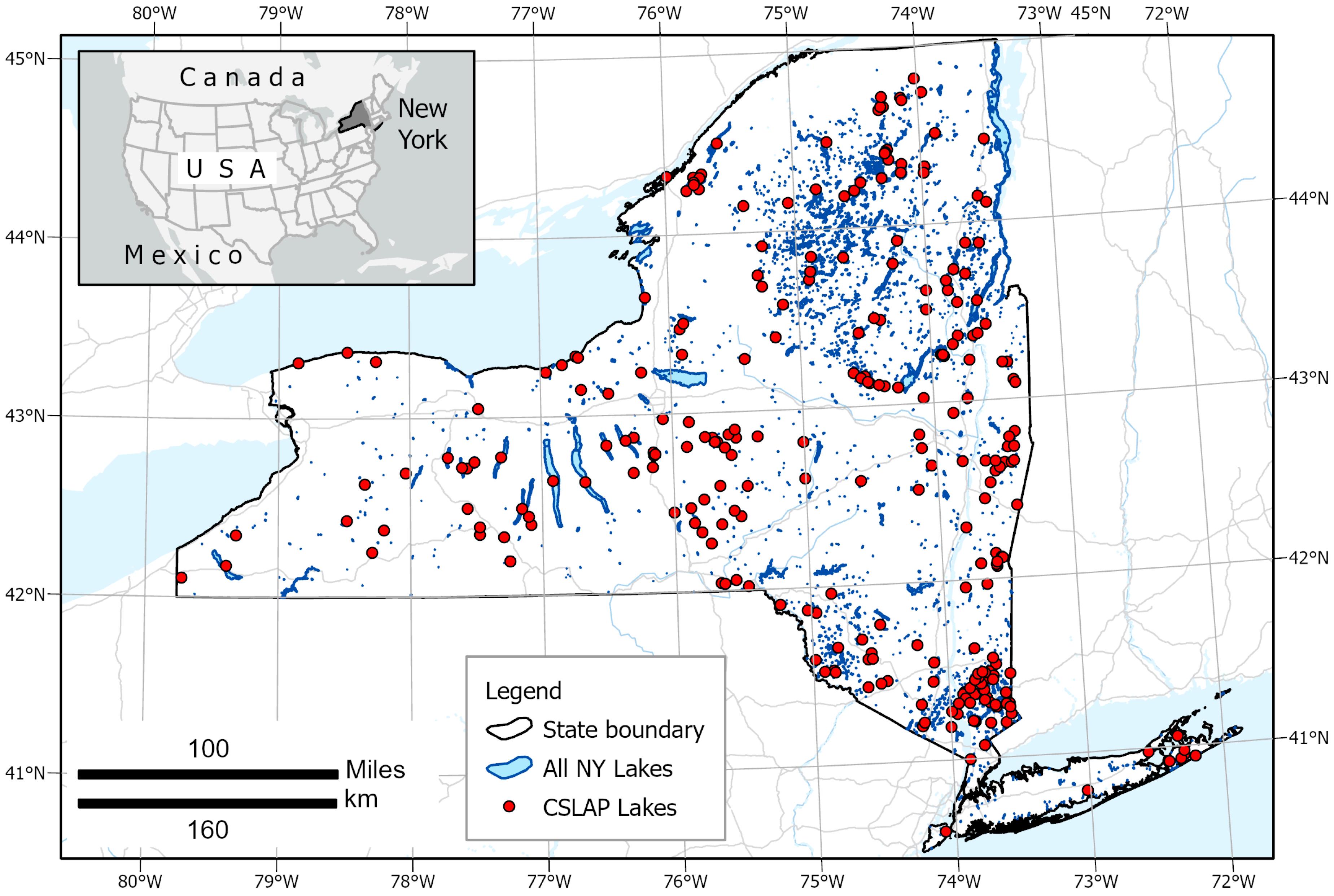
Figure 1. Study area: the red points indicate New York State lakes where in situ data were collected through the CSLAP program. Inset: New York State location in the USA.
Remotesensing 16 03504 g001
Figure 2. Flowchart of the various steps in the development of a retrieval model.
Remotesensing 16 03504 g002
Figure 3. Example of scatterplots between Chl-a and Sentinel-2 based 2BDA (RE1: band 5 and R: band 4) index with temporally matched in situ data and satellite data for (a) all in situ data, (b) in situ data above 8 μg/L.
Remotesensing 16 03504 g003
Figure 4. Scatterplot between in situ Chl-a above 8 μg/L and Sentinel-2-based 2BDA (RE1: band 5 and R: band 4) index with concurrent in situ and satellite data (blue points and line), one-day time window (orange points and line), and two-day time window (green points and line).
Remotesensing 16 03504 g004
Figure 5. Scatterplot between in situ phycocyanin concentration above 8 μg/L and Sentinel-2-based index.
Remotesensing 16 03504 g005
Figure 6. The prediction and confidence intervals (95%) for the MPH model based on (a) concurrent data model and (b) a one-day time window model. The X-axis shows the computed values from the satellite image (the spectral index) while the Y-axis shows the phycocyanin concentrations for the corresponding predicted values (blue line), the confidence and prediction interval limits (gray and green lines, respectively), and the in situ values, corresponding to the test data points (orange points). For example, an in situ point (highlighted with a red circle) corresponds to an MPH value of 0.033, which connects to an estimated phycocyanin value of 89.78 μg/L (red cross).
Remotesensing 16 03504 g006
Figure 7. Scatterplots between phycocyanin and Sentinel-2 index for training data based on applying Cloud Score+ (50% clear threshold) with total matched Sentinel-2 data and (a) all in situ data, (b) in situ data above 8 μg/L.
Remotesensing 16 03504 g007aRemotesensing 16 03504 g007b
Figure 8. Scatterplot between the predicted values and in situ measurements of phycocyanin concentration for the MPH model based on a concurrent testing dataset (2019 and 2020 CSLAP data) and Cloud Score+ processing. The five individually labeled points correspond to those in Figure 9 where the predictions of low phycocyanin concentrations did not match the moderate field phycocyanin concentrations (8–24 μg/L).
Remotesensing 16 03504 g008
Figure 9. Sentinel-2 images of five sample locations showing field samples (magenta marker) where points in the testing dataset predicted low phycocyanin concentrations despite high field concentrations (above 8 μg/L). Image source: https://www.sentinel-hub.com/explore/eobrowser/ (accessed on 24 April 2024).
Remotesensing 16 03504 g009aRemotesensing 16 03504 g009b
Table 1. Different indices derived from Sentinel-2 imagery for retrieval models.
IndexLabelEquation 1 Citation
Two-band Ratio2BDA R ( 705 ) R ( 665 ) [38]
Three-band Ratio3BDA 1 R ( 665 ) 1 R ( 705 ) × R ( 740 ) [63]
Normalized difference chlorophyll indexNDCI R ( 705 ) R ( 665 ) R ( 705 ) + R ( 665 ) [64]
Cyanobacteria indexCI [ ( R 665 R 560 ) 665 560 705 560 × ( R 705 R 560 ) ] [65]
Maximum chlorophyll indexMCI [ R 705 R 665 ] 705 665 740 665 × [ R 740 R 665 ] [66]
Maximum peak height MPH [ R 705 R 665 ] 705 665 865 665 × [ R 865 R 665 ] [67]
Surface algal bloom indexSABI ( R ( 865 ) R ( 665 ) ) ( R ( 490 ) + R ( 560 ) ) [68]
1 R(λ) is Sentinel-2 reflectance at wavelength λ: band 2 (490 nm), band 3 (560 nm), band 4 (665 nm), band 5 (705 nm), band 6 (740 nm), band 8A (865 nm).
Table 2. Comparison of R2, RMSE and MBE values for different phycocyanin (above 8 μg/L), models based on a concurrent (n = 27) and one-day window (n = 60) for the testing dataset (2019 and 2020). This is contrasted to the best Chl-a model (2BDA) for concurrent (n = 81) and one-day (n = 179) identified during the preliminary phase.
Chl-aPhycocyanin Index
Time WindowMetric2BDA2BDA3BDANDCICIMCIMPHSABI
Concurrent R20.430.420.130.400.450.300.630.002
RMSE2132.439.832.931.636.227.042.6
MBE0.66−0.27−1.430.42−1.02−1.510.34−1.96
One-day time windowR20.290.31−0.010.350.480.430.71−0.04
RMSE24.631.938.630.927.8292239.2
MBE−3.05−4.91−6.09−5.71−6.12−4.59−4.45−7.85
Table 3. Summary of linear models used for Chl-a and phycocyanin estimation (Using Sentinel-2 data filtered by QA60 bitmask).
ParameterTime WindowPrediction Model (µg/L)
Chl-aConcurrent43.78 × 2BDA − 25.860
Chl-aOne-day33.75 × 2BDA − 15.078
PhycocyaninConcurrent2486.33 × MPH + 7.146
PhycocyaninOne-day2191.88 × MPH + 6.891
Table 4. Accuracy assessment of estimation model based on CSLAP testing data, ESA QA60 bitmask cloud detection, with a division between points with low (<8 μg/L), moderate (8–24 μg/L), and high (>24 μg/L) concentration levels.
Chl-a PredictionPhycocyanin Prediction
Concurrent
n = 81
One-Day Time Window
n = 179
Concurrent
n = 27
One-Day Time Window
n = 60
FieldLowModerateHighLowModerateHighLowModerateHighLowModerateHigh
Moderate035151772611452294
High01120022530161024
Table 5. Comparison of R2 for MPH models based on different thresholds for Cloud Score+ (CSLAP phycocyanin 2019—concurrent data).
Cloud Score+ Threshold
30405060
All data0.62 (n = 359)0.67 (n = 321)0.68 (n = 263)0.62 (n = 196)
>8 μg/L0.81 (n = 42)0.86 (n = 40)0.87 (n = 32)0.80 (n = 27)
Table 6. R2, RMSE, and MBE for models of Chl-a and phycocyanin above 8 µg/l based on concurrent and one-day testing datasets (2019 and 2020).
Chl-a-2BDAPhycocyanin-MPH
Time WindownR2RMSEMBEnR2RMSEMBE
Concurrent 650.46622.5−1.96220.83914.9−3.87
One-day 1440.23124−1.2480.62318.3−1.91
Table 7. Summary of linear models used for Chl-a and phycocyanin estimation (using Sentinel-2 data filtered by Cloud Score+).
ParameterTime WindowPrediction Model (µg/L)
Chl-aConcurrent47.48 × 2BDA − 28.794
Chl-aOne-day37.36 × 2BDA − 17.712
PhycocyaninConcurrent3101.5 × MPH + 2.992
PhycocyaninOne-day3047.6 × MPH + 0.626
Table 8. Accuracy assessment of Chl-a and phycocyanin estimation models based on CSLAP testing data and Sentinel-2 data filtered by Cloud Score+, with a division between points with low (<8 μg/L), moderate (8–24 μg/L), and high (>24 μg/L) concentration levels.
Chl-a PredictionPhycocyanin Prediction
Concurrent
n = 65
One-Day Time Window
n = 144
Concurrent
n = 22
One-Day Time Window
n = 48
FieldLowModerateHighLowModerateHighLowModerateHighLowModerateHigh
Moderate02217166265948155
High0818014370040119
Disclaimer/Publisher’s Note: The statements, opinions and data contained in all publications are solely those of the individual author(s) and contributor(s) and not of MDPI and/or the editor(s). MDPI and/or the editor(s) disclaim responsibility for any injury to people or property resulting from any ideas, methods, instructions or products referred to in the content.