Snow Cover Extraction from Landsat 8 OLI Based on Deep Learning with Cross-Scale Edge-Aware and Attention Mechanism

Abstract

Snow cover distribution is of great significance for climate change and water resource management. Current deep learning-based methods for extracting snow cover from remote sensing images face challenges such as insufficient local detail awareness and inadequate utilization of global semantic information. In this study, a snow cover extraction algorithm integrating cross-scale edge perception and an attention mechanism on the U-net model architecture is proposed. The cross-scale edge perception module replaces the original jump connection of U-net, enhances the low-level image features by introducing edge detection on the shallow feature scale, and enhances the detail perception via branch separation and fusion features on the deep feature scale. Meanwhile, parallel channel and spatial attention mechanisms are introduced in the model encoding stage to adaptively enhance the model’s attention to key features and improve the efficiency of utilizing global semantic information. The method was evaluated on the publicly available CSWV_S6 optical remote sensing dataset, and the accuracy of 98.14% indicates that the method has significant advantages over existing methods. Snow extraction from Landsat 8 OLI images of the upper reaches of the Irtysh River was achieved with satisfactory accuracy rates of 95.57% (using two, three, and four bands) and 96.65% (using two, three, four, and six bands), indicating its strong potential for automated snow cover extraction over larger areas.

1. Introduction

Snow cover, as a crucial component of the cryosphere, is highly sensitive to climatic conditions and serves as a significant indicator of climate change [1,2]. It regulates the surface energy balance through the albedo effect. As snow cover diminishes, increased solar radiation absorption leads to localized warming, thereby accelerating the process of climate warming. Additionally, the retreat of snow cover may trigger the melting of permafrost, releasing substantial amounts of greenhouse gases and further advancing global climate change. In mountainous basins, snow cover is a vital water source, significantly influencing river runoff and freshwater supply [3]. Snowmelt serves as a crucial replenishment for many rivers, especially in arid or semi-arid regions, where the melting of snow delivers meltwater downstream, extending the water supply throughout spring and summer, which is essential for agricultural irrigation, urban water supply, and hydropower generation. However, as the climate warms and transitions from snow to rain in colder regions, the timing of snowmelt shifts earlier, reducing solid water storage in winter, and snowmelt and water flows move earlier in the season. This change can lead to increased risk of flooding in spring and exacerbate water scarcity in summer [4]. Therefore, understanding the distribution, storage, and melting of snow in mountainous regions with complex topography is crucial for effective water resource management, maintaining surface energy balance, and addressing regional climate change impacts [5,6,7].

Currently, snow cover analysis primarily depends on remote sensing data [8]. The evolution of snow cover monitoring algorithms has progressed from traditional visual interpretation to machine learning and deep learning [6,9,10]. Meanwhile, combining multiple data sources has led to significant progress in remote sensing data, particularly in temporal and spatial resolution [11]. However, when using optical remote sensing images for snow cover monitoring, the accuracy of snow cover identification tends to decrease as cloud coverage increases in some areas [12]. In addition, terrain has a significant impact on the distribution and accumulation of snow cover [13]. Mountains, canyons, and valleys can lead to shadow occlusion in remote sensing images [14]. The intermingling of different land cover types (e.g., snow cover, vegetation, rocks, forests) can lead to a complex blend of reflected signals [15]. Therefore, traditional thresholding methods and machine learning methods cannot fully extract useful information, making snow extraction still challenging [16], with various deep learning algorithms being increasingly applied.

In the realm of remote sensing for snow cover, mainstream deep learning algorithms primarily deploy architectures such as U-net [17] and DeepLabV3+ [18], often in conjunction with Transformer [19] architectures to boost performance. For instance, Wang et al. [20] assessed the U-net model’s performance in mapping snow cover using various Sentinel-2 image bands and discovered that bands B2, B4, B11, and B9 preserved almost all pertinent information for the clouds, snow, and background. They highlighted the challenges in differentiating snow from clouds, noting that resolving these complexities necessitates sophisticated models and superior data quality. Xing et al. [21] introduced a Partial Convolution U-Net (PU-Net) that leverages spatial and temporal data to reconstruct obscured NDSI values in MODIS snow products. The reconstructed pixels displayed Mean Absolute Errors ranging from 4.22% to 18.81% and Coefficients of Determination between 0.76 and 0.94 across various NDSI regions and coverage scenarios, underscoring the U-net model’s capability in snow detection via remote sensing. Nevertheless, Yin et al. [22], through comparative analyses involving threshold segmentation, U-net, Deeplabv3+, CDUnet, and their novel Unet3+ methods in cloud–snow discrimination trials, demonstrated that while U-Net and its enhancements surpass traditional approaches in accuracy, they still suffer from notable deficiencies such as inadequate long-range dependency and restricted receptive fields.

Simultaneously, facing challenges such as the multiscale features of snow in high-resolution remote sensing images, the similarity between clouds and snow, and occlusions caused by mountains and cloud shadows, Guo et al. [23] noted the scarcity and labor-intensive nature of obtaining pixel-level annotations for snow mapping in HSRRS images. They pre-emptively applied transfer learning techniques with the DeepLabv3+ network, achieving a snow extraction accuracy of 91.5% MIoU on a limited dataset, surpassing the 81.0% accuracy of a comparable FCN model. Kan et al. [24] introduced an edge enhancement module in the DSRSS-Net model, optimizing feature affinity loss and edge loss, which resulted in enhanced detailed structural information and improved edge segmentation for cloud–snow segmentation tasks. Relative to MOD10A1, the DSRSS-Net model’s snow classification accuracy and overall precision increased by 4.45% and 5.1%, respectively. Wang et al. [25] incorporated a Conditional Random Field (CRF) model into the DeepLabV3+ framework to overcome its limitations in distinguishing clouds and snow in GF-1 WFV imagery due to the absence of a short-wave infrared band sensor, noting a significant reduction in boundary blurring, slice traces, and isolated misclassifications. However, the DeepLabV3+ network’s complex structure contributes to its high computational demand. Additionally, Ding et al. [26] proposed the MAINet method, combining CNN and Transformer architectures in the final downsampling stage to minimize detail loss and clarify deep semantic features by reducing redundancy. Similarly, Ma et al. [27] used a dual-stream structure to merge information from Transformer and CNN branches, enhancing the model’s ability to differentiate between snow and clouds with similar spectral features during snow cover mapping using Sentinel-2 imagery, though further exploration of the model’s performance in practical applications is needed.

In summary, although different deep learning algorithms have been used for snow cover extraction, there is still great potential for improvement in terms of encoder–decoder structure and image structure information utilization, etc. Therefore, this study proposes a snow cover extraction method based on cross-scale edge-aware fusion and a channel-space attention mechanism in parallel with U-net. Section 2 offers a detailed overview of the two types of datasets used for experimental evaluation, as well as the specific methodologies employed in the models’ construction and the experimental environments and parameter configurations for each model. Section 3 displays the experimental results of the models across various datasets from multiple angles, as well as the ablation study outcomes of the CEFCSAU-net model. Section 4 visualizes and deeply analyzes the features extracted from the CSA and CEF modules, examines the limitations of the models discussed in this paper in applying multi-source remote sensing data, and outlines future research strategies and directions. Finally, Section 5 summarizes the application prospects and principal findings of the experimental results of the models discussed in this paper.

2. Materials and Methods

2.1. Experimental Dataset

The datasets evaluated in this study include the publicly available CSWV_S6 dataset and Landsat8 OLI dataset, respectively.

2.1.1. CSWV_S6 Dataset

The CSWV dataset [28] is a freely and publicly available dataset constructed by Zhang et al., based on synthesizing WorldView2’s red, green, and blue bands. The dataset was taken in the Cordillera Mountains of North America, and the distribution of clouds and snow was obtained based on the interpretation of WorldView2 images from June 2014 to July 2016. This study utilizes the CSWV_S6 data with a spatial resolution of 0.5 m (Figure 1), available at https://github.com/zhanggb1997/CSDNet-CSWV (accessed on 14 September 2024). The area depicted in the image comprises forests, grasslands, lakes, and bare ground, among others. In the dataset, clouds and snow were labeled, but only the snow labels were used in this study to classify features into snow and non-snow categories.

2.1.2. Landsat 8 OLI Dataset

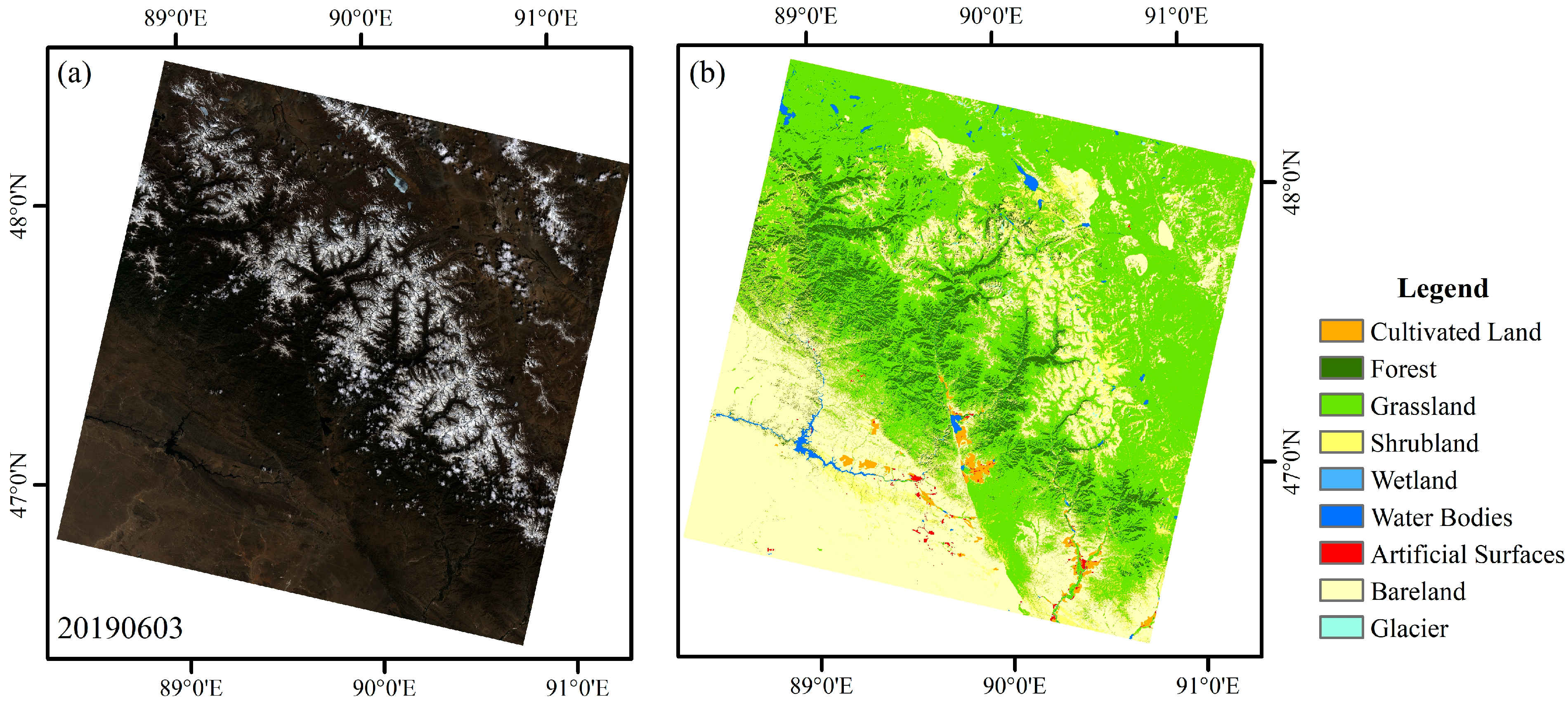
Landsat 8 OLI imagery offers a spatial resolution of 30 m, with the OLI sensor comprising nine bands, including three visible, infrared, and short-wave infrared bands, among others. To minimize cloud interference during snow extraction, we selected six Landsat images with cloud coverage of less than 30% from dates “20180413”, “20180515”, “20190315”, “20190603”, “20200317”, and “20200402”. Figure 2 presents an overview of the study area, with complete data available at https://zenodo.org/records/12635483 (accessed on 14 September 2024). In the methodological experimentation phase, bands 2 (blue), 3 (green), and 4 (red) were selected to construct the dataset for comparative analysis against the public dataset (CSWV_S6). For labeling, bands 3 (green), 5 (NIR), and 6 (SWIR 1) were utilized. Additionally, recognizing the significance of the short-wave infrared band for snow detection, the study incorporated SWIR 1 (band 6) as an input feature in the discussion phase experiments. This was done to compare the efficacy of solely using bands 2, 3, and 5 and to delve deeper into the benefits of multispectral data fusion for improving the performance of remote sensing image processing algorithms.

2.2. Data Processing

First, radiometric calibration and atmospheric correction were performed on Landsat 8 OLI image data. Snow cover was then extracted using the SNOMAP algorithm by calculating the Normalized Difference Snow Index (NDSI) with the short-wave infrared and green bands of the Landsat images [29]. In experiments, pixels were extracted as snow cover if they had an NDSI of 0.4 or higher, and the near-infrared reflectance threshold was increased to 0.11 or higher to reduce the misclassification of water bodies. Additionally, pixels that were either not identified or misidentified by the SNOMAP algorithm were corrected through visual interpretation to accurately determine the snow cover extent within the study area as label data.

Then, due to the limitations in computational resources and model architecture when processing large-scale data, large-size remote sensing images were divided into multiple fixed-size chunks [30]. Therefore, the study utilized the sliding window method to segment the six-image views of CSWV_S6 data, Landsat 8 OLI data, and the corresponding labeled data to create an input dataset that meets the model’s required size. Here, a fixed-size sliding window of 512 × 512 pixels was established, and the sliding window moved along the horizontal and vertical directions on each remote sensing image, advancing a fixed step each time. In this manner, the entire remote sensing image was gradually covered. The CSWV_S6 image data comprised 1114 windows of 512 × 512 size, while the Landsat 8 OLI image data included 1260 windows of the same size, with corresponding labeling data for each.

The homemade experimental data underwent a secondary screening, with datasets containing 10% to 90% snow pixels selected to focus the study on snow-covered scenes. Ultimately, from the 1260 original window datasets of Landsat data, 413 that met the criteria were selected. For the 1114 raw window datasets of CSWV_S6 data, to minimize screening interference and emphasize generalization capabilities, snow-free datasets were excluded, resulting in 688 valid datasets being selected. This approach not only ensures the relevance of the data to the study’s objectives but also enhances the robustness of the findings by covering a wide range of snow conditions.

Following the data preprocessing outlined above, the labels and individual band data were stored in single-channel .tif format, with dimensions of (512, 512, 1). To boost data processing efficiency, streamline the preprocessing workflow, and enhance compatibility with deep learning frameworks, the data in .tif format were converted to .npy format. Additionally, all image data were normalized, scaling pixel values to the range [0,1]. The converted label data retained its shape (512, 512, 1), while the Landsat 8 OLI data were stored in the following multi-channel formats: (512, 512, 3) and (512, 512, 4). Similarly, the CSWV_S6 data were converted into a (512, 512, 3) .npy format. This conversion step ensured the data were efficiently processed and readily usable in subsequent deep learning models.

Finally, the valid data were divided into training, validation, and test sets in the ratio of 7:2:1. Additionally, for deep learning model training, sample size is typically a critical consideration. To ensure that the deep learning model could learn a sufficient number of features and patterns, this experiment applied horizontal and vertical flips to the data inputs with a 50% probability during each cycle of the training and validation phases. This technique enhanced the robustness of the model by augmenting the variability of training examples without requiring additional raw data.

2.3. Deep Learning Models

2.3.1. Model Architecture

We propose a cross-scale edge-aware fusion and channel spatial attention mechanism parallelization-based snow cover extraction method on the U-net model architecture (Cross-Scale Edge-Aware Fusion and Channel Spatial Attention Mechanism Parallelization, CEFCSAU-net) (Figure 3). First, an enhanced parallel Channel Spatial Attention Mechanism (CSA) is employed during the encoding stage of model feature extraction to adaptively enhance the model’s attention to key features and improve the efficiency of global semantic information utilization [31]. Second, the proposed Cross-Scale Edge-Aware Fusion (CEF) module replaces the original skip connections in U-net, enhancing low-level image features through multiple edge detection at shallow scales and improving detail perception through the separation and fusion of features at deeper scales [32]. Additionally, Batch Normalization (BN) is applied after each convolutional stage to accelerate training and stabilize the gradients [33].

Additionally, the model’s output is provided as “logits”, which facilitate the calculation of the loss function. These logits represent raw, unbounded predictive values, produced directly by the final layer of the model without applying an activation function. They reflect the model’s confidence in each pixel belonging to a specific category. In binary classification tasks, each pixel’s final classification is determined by applying a zero threshold to these logits. Specifically, if the value of logits exceeds zero, the pixel is classified as the target class (snow); otherwise, it is classified as the background or other categories (non-snow). This approach enables the model to classify effectively based on the sign and magnitude of the logits, eliminating the need for additional nonlinear transformations. Ultimately, following this post-processing, the output data from the test set are stored in PNG format with dimensions of (512, 512, 1).

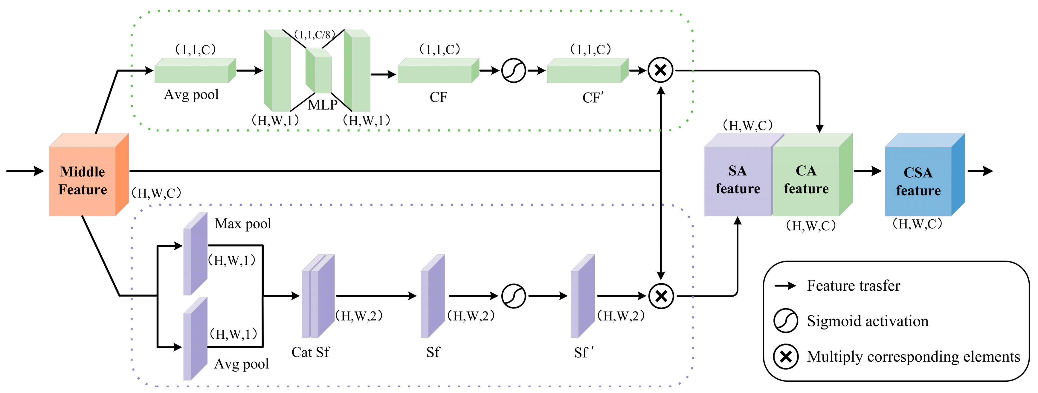
2.3.2. Channel Spatial Attention Mechanism Parallel Module (CSA)

The parallel channel space attention mechanism modules (Figure 4) are introduced during the encoding phase of model feature extraction, which adaptively enhance the model’s attention to key features and improve the efficiency of utilizing global semantic information.

The channel attention mechanism [34] in the upper branch of the CAS module primarily concentrates on the weights assigned to different channels in the input feature map, aiding the model in better learning the correlations among features and enhancing the model’s representational capacity.

The spatial attention mechanism in the lower branch primarily concentrates on the weights assigned to different locations in the input feature map, thereby honing the model’s focus on crucial spatial locations and enhancing its capacity to perceive spatial structures [35]. This combined approach enhances the model’s capacity to process input features, thereby boosting its performance and generalization capabilities. The calculation formula is as follows:

$$\mathrm{C}{\mathrm{A}}_{\mathrm{f}}=\mathrm{X}\otimes \mathrm{Softmax}\left(\mathrm{MLP}\left(\mathrm{AvgPool}\left(\mathrm{X}\right)\right)\right)$$

(1)

$$\mathrm{Sf}=\mathrm{Con}{\mathrm{v}}_{1\times 1}\left(\mathrm{Concat}\left(\mathrm{MaxPool}\left(\mathrm{X}\right),\mathrm{AvgPool}\left(\mathrm{X}\right)\right)\right)$$

(2)

$$\mathrm{S}{\mathrm{A}}_{\mathrm{f}}=\mathrm{X}\otimes \mathrm{Softmax}\left(\mathrm{Con}{\mathrm{v}}_{1\times 1}\left(\mathrm{Sf}\right)\right)$$

(3)

$$\mathrm{CS}{\mathrm{A}}_{\mathrm{f}}=\mathrm{Con}{\mathrm{v}}_{1\times 1}\left(\mathrm{Concat}\left(\mathrm{C}{\mathrm{A}}_{\mathrm{f}},\mathrm{S}{\mathrm{A}}_{\mathrm{f}}\right)\right)$$

(4)

2.3.3. Cross-Scale Edge-Aware Fusion Module (CEF)

The cross-scale edge-aware fusion module (Figure 5) replaces the traditional skip connections in the U-net model. The aim is to enhance low-level image features by introducing multiple edge detection on shallow feature scales and to improve detail perception through branch separation and fusion of features on deep feature scales.

In the CEF module, image feature information is initially captured on shallow feature scales using Sobelx, Sobely, and Laplacian operations [36]. Among them, Sobelx and Sobely operations detect horizontal and vertical edges, while the Laplacian operation enhances high-frequency details [24]. These operations are processed in parallel and combined to enhance the model’s sensitivity to image edges and textures, as well as to improve feature differentiation. The computation and output equations are as follows:

$$\mathrm{X}\mathrm{’}=\mathrm{Con}{\mathrm{v}}_{1\times 1}\left(\mathrm{X}\right)$$

(5)

$$\mathrm{SS}{\mathrm{L}}_{\mathrm{f}}=\mathrm{Conv}\left({\mathrm{X}}^{\prime },\mathrm{kerne}{\mathrm{l}}_{\mathrm{x}}\right)+\mathrm{Conv}\left({\mathrm{X}}^{\prime },\mathrm{kerne}{\mathrm{l}}_{\mathrm{y}}\right)+\mathrm{Conv}\left({\mathrm{X}}^{\prime },\mathrm{kerne}{\mathrm{l}}_{\mathrm{L}}\right)$$

(6)

$$\mathrm{kerne}{\mathrm{l}}_{\mathrm{x}}=\left[\begin{array}{ccc}-1& 0& 1\\ -2& 0& 2\\ -1& 0& 1\end{array}\right],\mathrm{kerne}{\mathrm{l}}_{\mathrm{y}}=\left[\begin{array}{ccc}-1& -2& -1\\ 0& 0& 0\\ 1& 2& 1\end{array}\right],\mathrm{kerne}{\mathrm{l}}_{\mathrm{L}}=\left[\begin{array}{ccc}0& 1& 0\\ 1& -4& 1\\ 0& 1& 0\end{array}\right]$$

(7)

where Conv denotes the convolution operation, kernel_x, kernel_y, and kernel_L denote the convolution kernels for Sobelx, Sobely, and Laplacian operations, respectively, and SSL_f is the new feature map after their summation. The new feature map is then used to generate the edge-sensing features through a series of operations: the edge-sensing feature (Es_f).

$$\mathrm{DF}=\mathrm{Upsample}\left(\mathrm{RELU}\left(\mathrm{BN}\left(\mathrm{Con}{\mathrm{v}}_{1\times 1}\left({\mathrm{Y}}_{\mathrm{f}}\right)\right)\right)\right)$$

(8)

$$\mathrm{C}{\mathrm{s}}_{\mathrm{f}}=\mathrm{Con}{\mathrm{v}}_{3\times 3}\left(\mathrm{X}\right)+\mathrm{RELU}\left(\mathrm{BN}\left(\mathrm{Con}{\mathrm{v}}_{1\times 1}\left(\mathrm{X}+\mathrm{DF}\right)\right)\right)$$

(9)

$${\mathrm{D}}_{\mathrm{f}}=\mathrm{X}-\mathrm{DF}$$

(10)

$$\mathrm{Ou}{\mathrm{t}}_{\mathrm{f}}=\mathrm{E}{\mathrm{s}}_{\mathrm{f}}+\mathrm{C}{\mathrm{s}}_{\mathrm{f}}+{\mathrm{D}}_{\mathrm{f}}$$

(11)

2.4. Snow Extraction

2.4.1. Experimental Configuration

Before conducting experiments with the research model described in this paper, establishing the appropriate experimental environment is essential. Currently, the software environment for the model in this paper is configured with the “Windows 11, version 22H2” operating system, “Python 3.8” version, and the “PyTorch 1.7.1+cu110” deep learning framework. The hardware environment features a “CPU: 12th Gen Intel Core i7-12700K” and a “GPU: NVIDIA GeForce RTX 3090”.

During the model’s construction and training phases, it was trained on a GPU device, with the number of training cycles (epochs) uniformly set at 50, batch size at 8, and worker threads in the data loader also at 8. In each training cycle, BCEWithLogitsLoss [37] was used as the loss function, with its formula provided in Equations (12) and (13).

$$\mathsf{\sigma }\left({\mathrm{x}}_{\mathrm{i}}\right)=\mathrm{Sigmoid}\left(\mathrm{x}\right)={\displaystyle \frac{1}{1+{\mathrm{e}}^{-{\mathrm{x}}_{\mathrm{i}}}}}$$

(12)

$$\mathrm{BCE}{\mathrm{W}}_{\mathrm{Loos}}=-{\displaystyle \frac{1}{\mathrm{N}}}{\sum }_{\mathrm{i}=1}^{\mathrm{N}}\left[{\mathrm{y}}_{\mathrm{i}}\cdot \log \left(\mathsf{\sigma }\left({\mathrm{x}}_{\mathrm{i}}\right)\right)+\left(1-{\mathrm{y}}_{\mathrm{i}}\right)\cdot \log \left(1-\mathsf{\sigma }\left({\mathrm{x}}_{\mathrm{i}}\right)\right)\right]$$

(13)

where N is the number of samples; y_i is the true label of sample i, which takes the value of 0 or 1; x_i is the prediction result of sample i; and the log function is the natural logarithm.

In addition, the experiment employs the Adam optimizer for parameter updates, with an initial learning rate (α) of 0.0001, a first-order momentum decay rate (β₁) of 0.5, and a second-order momentum decay rate (β₂) of 0.99, facilitating faster convergence and enhanced performance of the model.

To compare the performance of different models under uniform experimental conditions, enhancing comparability and consistency, this paper standardized the hyperparameter settings of the FCN8s [38], SegNet [39], U-net [17], and DeepLabV3+ [18] models. Specifically, FCN8s based on the VGG16 architecture employ a fully convolutional network (FCN) that integrates features from various levels via skip connections. SegNet features a classic encoder–decoder architecture, with the encoder identical to VGG16 and the decoder progressively upsampling to restore spatial resolution. U-net is known for its symmetrical U-shaped structure, which utilizes skip connections to directly transfer features from the encoder to the decoder. DeepLabV3+ employs ResNet50 as its backbone network, expanding the receptive field by incorporating atrous convolution and an ASPP module, capturing multi-scale features.

2.4.2. Assessment of Indicators

To objectively evaluate the prediction accuracy of the model at the image pixel level and its ability to recognize snow categories, four metrics were selected to evaluate the model’s performance in this study: Pixel Accuracy (PA), Recall (R), F1 Score (F1), and Mean Intersection over Union (MIoU) [28]. The formulas for these metrics are as follows:

$$\mathrm{P}\mathrm{A}={\displaystyle \frac{\mathrm{T}\mathrm{P}+\mathrm{T}\mathrm{N}}{\mathrm{T}\mathrm{P}+\mathrm{T}\mathrm{N}+\mathrm{F}\mathrm{P}+\mathrm{F}\mathrm{N}}}$$

(14)

$$\mathrm{P}={\displaystyle \frac{\mathrm{TP}}{\mathrm{TP}+\mathrm{FP}}}$$

(15)

$$\mathrm{R}={\displaystyle \frac{\mathrm{T}\mathrm{P}}{\mathrm{T}\mathrm{P}+\mathrm{F}\mathrm{N}}}$$

(16)

$$\mathrm{F}1=2\cdot {\displaystyle \frac{\mathrm{P}\mathrm{*}\mathrm{R}}{\mathrm{P}+\mathrm{R}}}$$

(17)

$$\mathrm{I}\mathrm{o}{\mathrm{U}}_{\mathrm{i}}={\displaystyle \frac{\mathrm{T}{\mathrm{P}}_{\mathrm{i}}}{\mathrm{T}{\mathrm{P}}_{\mathrm{i}}+\mathrm{F}{\mathrm{P}}_{\mathrm{i}}+\mathrm{F}{\mathrm{N}}_{\mathrm{i}}}}$$

(18)

$$\mathrm{M}\mathrm{I}\mathrm{o}\mathrm{U}={\displaystyle \frac{1}{\mathrm{N}}}{\sum }_{\mathrm{i}=1}^{\mathrm{N}}\mathrm{Io}{\mathrm{U}}_{\mathrm{i}}$$

(19)

where PA is the ratio of the number of pixels correctly categorized at all pixel levels to the total number of pixels, TP denotes true cases, TN denotes true-negative cases, FP denotes false-positive cases, and FN denotes false-negative cases. IoU_i denotes the intersection and concatenation ratio of the ith category, and N denotes the total number of categories.

3. Experimental Results

3.1. Experimental Results for CSWV_S6 Data

Table 1. Comparison of mean values of different segmentation models on CSWV_S6 test set data.

Model	PA (%)	R (%)	F1 (%)	mIoU (%)
FCN8s	96.31	71.86	69.96	75.69
SegNet	94.99	79.42	76.9	78.56
U-net	96.34	72.29	74.54	79.03
DeepLab V3+	97.51	82.38	81.40	83.77
CEFCSAU-net	98.14	87.87	85.62	86.28

Note: The bold text in the table represents the maximum value of the indicator in that column.

presents the average results for all evaluation metrics in the test set. It is evident that the models differ in terms of pixel accuracy (PA), recall (R), F1 score, and mean intersection over union (mIoU). The CEFCSAU-net model outperforms other models across all indices, particularly in pixel accuracy, achieving 98.14% and demonstrating high segmentation accuracy and consistency on CSWV_S6 data.

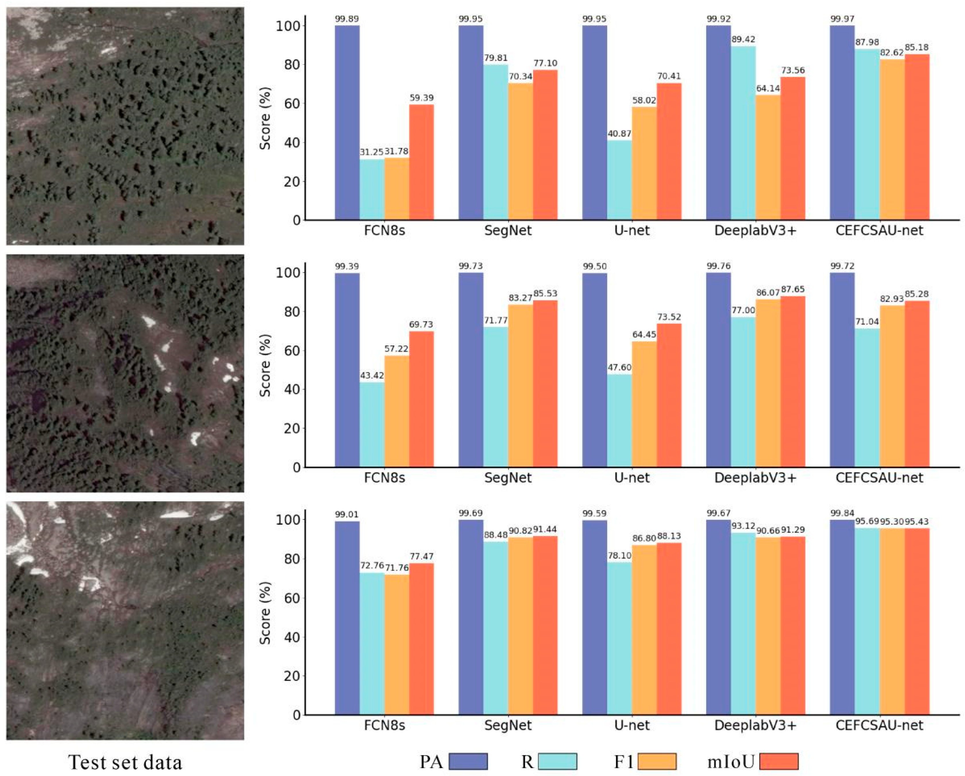
Simultaneously, three images from the CSWV_S6 test set, featuring snow cover ranging from 10% to 90%, were selected (Figure 6). The results indicate that among the FCN8s, SegNet, U-net, DeepLabV3+, and CEFCSAU-net models, the CEFCSAU-net exhibits the fewest segmentation errors.

3.2. Experimental Results on Landsat8 OLI Data

Table 2. Comparison of mean values of evaluation metrics on different segmentation models for Landsat test set data.

Model	PA (%)	R (%)	F1 (%)	mIoU (%)
FCN8s	85.65	80.95	83.62	68.24
SegNet	92.36	91.99	92.42	82.09
U-net	91.89	93.68	91.89	81.26
DeepLab V3+	92.68	92.91	92.39	81.79
CEFCSAU-net	95.67	96.68	95.74	88.68

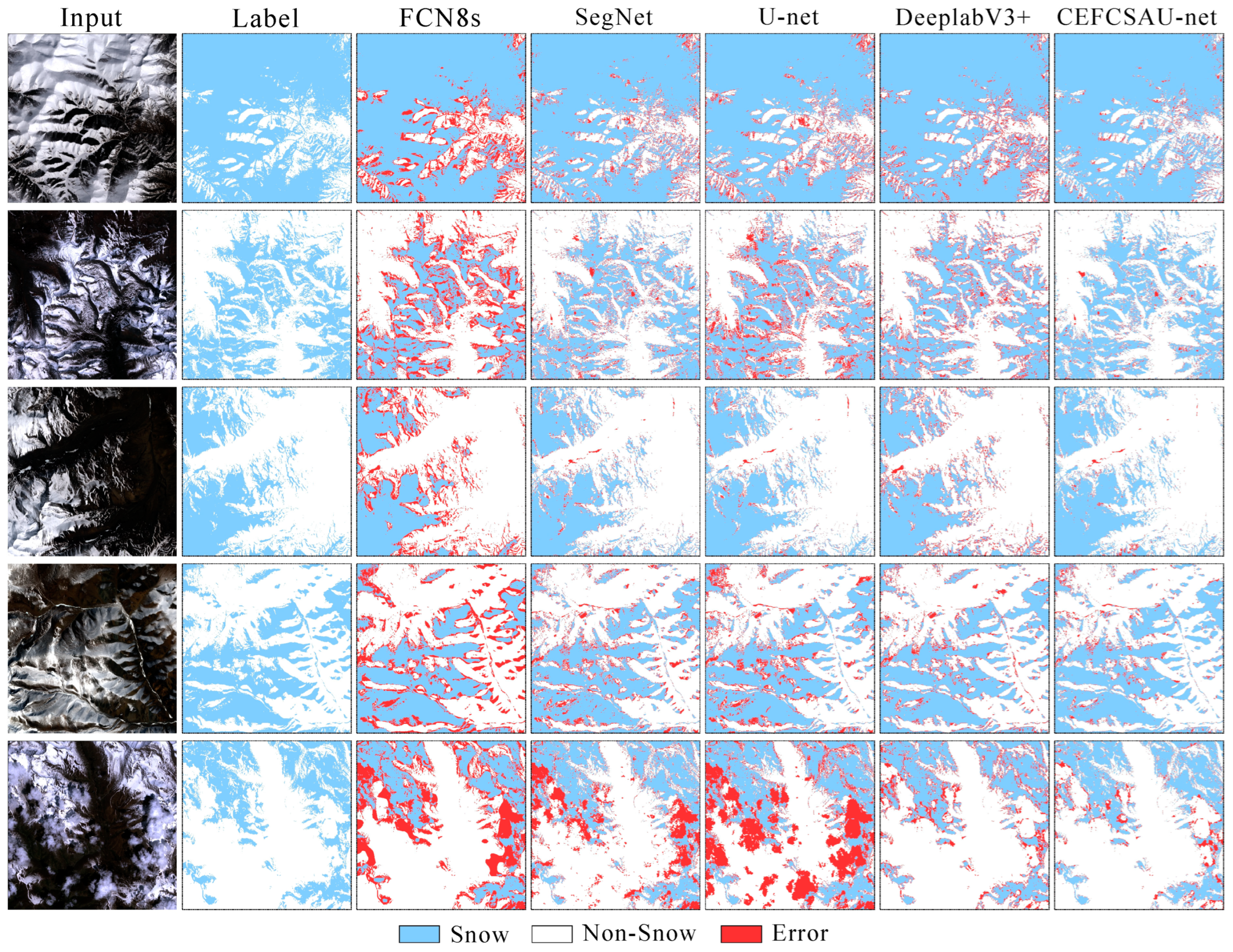
Note: The bold text in the table represents the maximum value of the indicator in that column.

displays the performance of each model on the snow cover extraction task, based on experiments with various segmentation models on the self-created Landsat 8 OLI dataset. The experimental results reveal that the CEFCSAU-net model achieves the highest scores across all metrics, underscoring its superior performance in snow extraction. Combining some of the test samples (Figure 7) shows that the overall performance results of each model align with those of the CSWV_S6 data.

Furthermore, in scenes with high cloud content, like those in the fifth row, the FCN8s, SegNet, and U-net models frequently misclassify significant amounts of clouds as snow. In contrast, the DeepLabV3+ and CEFCSAU-net models effectively identify clouds as non-snow features. The CEFCSAU-net model, however, retains a keen perception of snow edges, reflecting its high accuracy and robustness in snow extraction. This analysis illustrates the relative strengths and weaknesses of the different models under varied environmental conditions.

3.3. Model Comparison and Analysis

Several studies have carried out snow cover monitoring with pixel-level convolutional neural network algorithms [23,40,41], finding that their powerful feature learning capabilities, adaptability to complex textures, and processing of temporal information lead to more accurate, automated, and efficient monitoring and analysis of snow cover [42]. In conjunction with Section 3.1 and Section 3.2, we compare and analyze several models selected in the experiment.

The experimental findings are as follows: the FCN8s model, featuring a full convolutional network structure, fails to fully utilize edge detail information, resulting in poor edge effects and a high number of erroneous detections. It also performs poorly across various evaluation metrics. The SegNet and U-net models, which utilize an encoder–decoder structure, improve the retention of edge detail information. However, they still lack spatial information, resulting in fewer edge detail misdetections compared to the FCN8s model, but with more widespread misdetection areas.

Meanwhile, the DeepLabV3+ model, which contains pyramid pooling and atrous convolution structures, achieves multi-scale feature extraction and integration. This, combined with fusion with low-level feature maps, restores the spatial details of the segmentation results and performs more stably across all evaluation metrics.

Finally, compared to the other four models, the CEFCSAU-net model introduces the CSA module, which adaptively enhances the model’s focus on key features and improves the utilization of global semantic information. Additionally, the original skip-connected CFE module of U-net is replaced to enhance cloud–snow differentiation and edge perception through multiple edge detection and branch separation and fusion features, ultimately achieving the best performance results.

3.4. Indicator Fluctuations Due to Data Discrepancies

From the experimental results of the previous CEFCSAU-net model on CSWV_S6 data and Landsat8 OLI data, the indicators of PA, R, F1, and mIoU are higher than other models. Furthermore, the results of the ablation experiments confirm that the incremental integration of the CSA and CEF modules into the U-net model effectively enhances its performance. Meanwhile, by comparing the boxplots of various indicators of different models on the two sets of data in Figure 8, it can be found that the indicator scores of the CEFCSAU-net model for the whole test set of data are stable, compact, and uniformly distributed compared with the other four models. This further confirms the significant role of the improvement measures discussed in this paper in enhancing model performance.

However, as depicted in Figure 8, the fluctuation range for the R, F1, and mIoU metrics in Figure 8a is substantially greater than for the PA metrics, with more outliers observed for each model than in Figure 8b. Analysis of each model’s results in the test set revealed that the metric fluctuations stemmed from data variations, notably because the CSWV_S6 dataset excluded no-snow data during processing, leading to a higher presence of data with a lower percentage of snow image elements. The scores of the evaluation metrics for each model on three CSWV_S6 test set examples are displayed in Figure 9, illustrating how this type of data induces minor errors in recognizing snow image elements, thereby causing significant fluctuations in the scores of the R, F1, and mIoU metrics.

Nevertheless, the performance of CEFCSAU-net in Figure 9 is still satisfactory. It shows that the study’s data processing of CSWV_S6 did not lead to the emergence of the category imbalance problem, but rather verified the reliability of the CEFCSAU-net model.

3.5. Differences in the Extraction of Cloud–Snow Confusion Scenarios

As is well known, distinguishing between snow, clouds, and cloud shadows is a crucial step in remote sensing processing [23]. Yao et al. [43] introduced the CD-AttDLV3+ network, which employs channel attention and demonstrates outstanding performance in distinguishing clouds from bright surfaces and detecting translucent thin clouds, providing valuable insights. 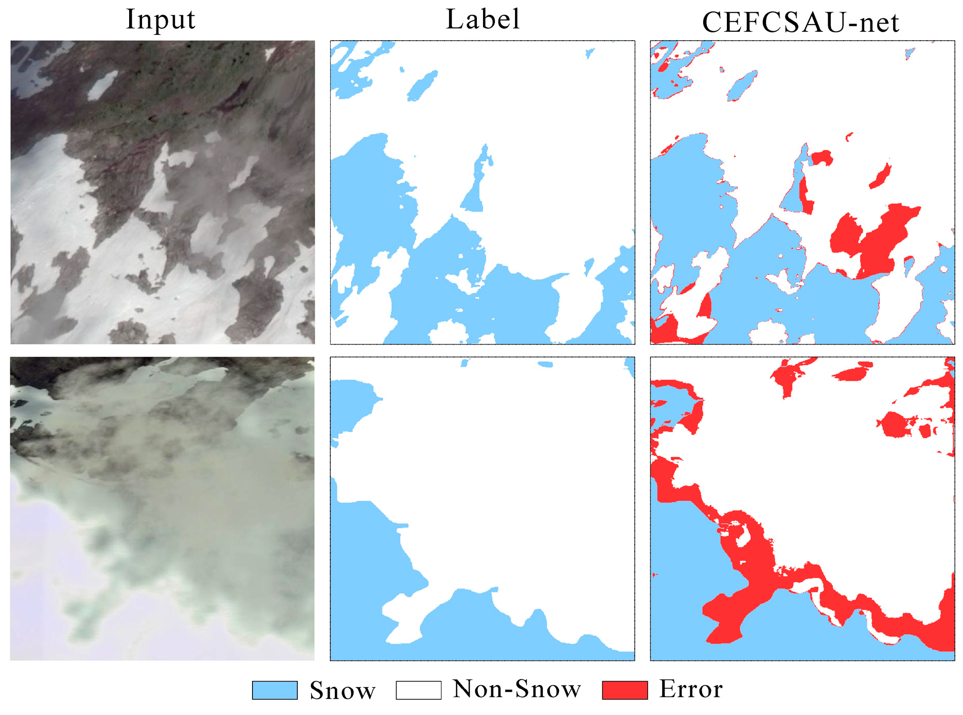In Section 3.1 and Section 3.2, Figure 6 and Figure 7 illustrate that the CEFCSAU-net model has fewer error detection regions than the other models, both on the edges and in the details. However, the CEFCSAU-net model, while generally stable, shows an increased red error detection region in scenes with high cloud coverage, as seen in the fifth row of Figure 7. Analysis of the input image reveals that this error region primarily originates from the overlap of clouds and snow.

In addition, while the CDnet proposed by Yang et al. introduces edge refinement operations, it encounters pixel omission issues in thin cloud extraction [44]. Figure 10 shows that the CEFCSAU-net model demonstrates capabilities in detecting snow under thin clouds and effectively distinguishing large areas of thick clouds, though it sometimes struggles with the boundaries of thick clouds. This indicates that even the high-performing CEFCSAU-net model experiences increased false detections in areas with cloud–snow confusion.

3.6. Ablation Experiments

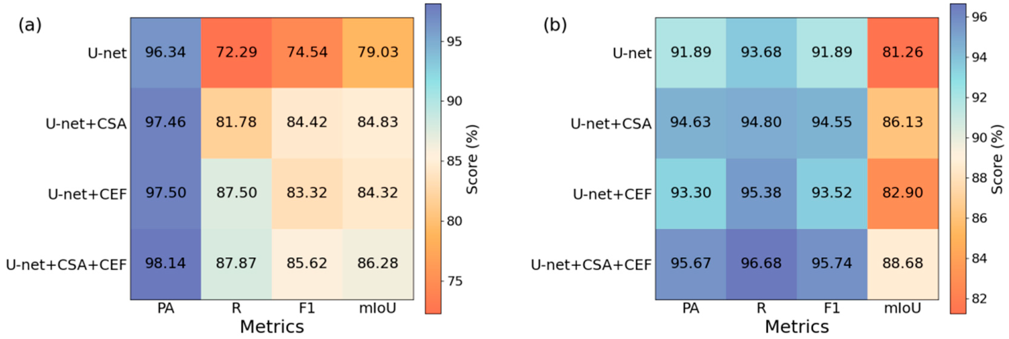
In deep learning modeling research, ablation experiments quantify the importance of specific components, hierarchies, parameters, or input features of a model by gradually modifying or removing them on model functionality, performance, or robustness [45]. In this experiment, ablation experiments were conducted for both the CSA module and the CEF module on both the CSWV_S6 dataset and the Landsat 8 OLI dataset in order to observe and compare the performance under different model configurations, and the experimental correlation results are shown in Figure 11 below.

From the perspective of model design principles and architecture, the parallel channel and spatial attention mechanisms focus on the correlations among different channels and the spatial connections among various locations in the input feature map, respectively, in order to improve the model’s representation ability and perception of spatial structure, as well as to improve the model’s processing of the input features and thus the accuracy of classification. The experimental results show that the introduction of the CSA module on the CSWV_S6 dataset improves the PA, R, F1, and mIoU by 1.12%, 9.49%, 9.88%, and 5.8%, respectively. On the Landsat 8 OLI dataset, these metrics improved by 2.74%, 1.12%, 2.66%, and 4.87%, respectively, demonstrating the CSA module’s effectiveness.

Additionally, low-level image features are enhanced by introducing multiple edge detections on the shallow feature scale, as well as the cross-scale CEF module, which obtains detailed features through feature fusion and separation after upsampling on the deep feature scale. Following its introduction, the CEF module also improved various evaluation metrics on the CSWV dataset: PA by 1.16%, R by 15.21%, F1 by 8.78%, and mIoU by 5.29% compared to the U-net model. On the Landsat 8 OLI dataset, improvements were PA by 1.41%, R by 1.7%, F1 by 1.63%, and mIoU by 1.64%, indicating the CEF module’s effectiveness.

Finally, the CEFCSAU-net model, which achieved optimal results and significant enhancements across all metrics, demonstrates that when both the CSA and CEF modules are introduced, the features enhanced by the CSA module are further enhanced by the cross-scale CEF module. This synergy results in improved outcomes with reduced information loss in differential features.

4. Discussion

4.1. Contribution Analysis of CSA and CEF Modules

To gain a deep understanding of the roles and contributions of the CSA and CEF modules in the feature extraction process, this paper visualized the intermediate features extracted by these modules as heatmaps to facilitate an intuitive observation of the important information captured by these modules during data processing [46].

CSA Module Contribution Analysis: The CSA module enhances key feature expressions by focusing on both the channel and spatial dimensions of the feature maps. Considering the number of channels in the intermediate feature maps, this study visualized only the first eight channels of the feature maps before and after the first application of the CSA module (total number of channels: 64). In Figure 12b, it is evident that half of the channel feature maps were not effectively distinguished, while the other half showed only subtle differences. However, in Figure 12c, each channel’s feature map is effectively distinguished, and significant differences are observed between the channels. These results demonstrate how the CSA module’s channel attention mechanism enhances and suppresses various channels and how its spatial attention mechanism discriminates the information across feature maps. This selective attention allows the model to utilize key features more accurately in subsequent layers, thereby enhancing overall performance.

CEF Module Contribution Analysis: The CEF module captures edge features and enhances detail perception by extracting cross-scale features. In experiments, with Figure 12a as input and by manipulating the presence of the CSA and CEF modules, the value of the CEF module is assessed. In Figure 13, it is evident that the feature maps b1–b4 for snow and non-snow edges are significantly enhanced compared to a1–a4, demonstrating the model’s sustained sensitivity to spatial features with scale changes. This illustrates the CEF module’s strong structural capability in spatially enabling the model to more effectively capture the geometric shapes and contours of key features in the input data.

Combined Contribution Analysis and Limitations of CSA and CEF Modules: As observed, feature maps c1 and c2 in Figure 13 offer superior performance in detailing edges and spatial attributes compared to a1, a2, b1, and b2, providing the model with a more comprehensive capability for feature expression. However, feature maps at stages c3 and c4 show less spatial detail in the upper right areas than a3, a4, b3, and b4. This may be attributed to the feature maps being represented as channel averages, which do not effectively showcase the distinct contributions of each channel in a collaborative state. Additionally, the abundance of channels in the network’s deeper stages and the successive normalizations may reduce feature value distinctions, diminishing module performance.

In conclusion, the CSA and CEF modules play an indispensable role in the feature extraction process. For a more detailed analysis of the value and role of different modules within the model, considering the mechanics of remote sensing imagery and integrating multispectral data for further targeted, quantitative analysis and exploration are necessary.

4.2. Limitation and Prospects

The snow cover extraction method described in this paper, based on cross-scale edge perception and attention mechanisms, is implemented on the U-net model architecture. This approach addresses the issues of inadequate local detail perception and insufficient global semantic information utilization in existing methods by incorporating the CSA and CEF modules. Furthermore, it demonstrates potential in detecting snow under thin clouds. However, due to the limitations inherent in optical remote sensing images, the current CEFCSAU-net model still faces challenges with cloud–snow confusion scenarios, revealing some limitations and shortcomings.

Additionally, in traditional snow detection methods, the SWIR band of the NDSI plays a crucial role [47]. Consequently, this study specifically incorporated the SWIR band in analyzing Landsat data to assess its impact on the performance of deep learning models. The experimental results are shown in

Table 3. Comparison of the mean values of different segmentation model evaluation metrics on the test set after the introduction of SWIR 1 band to Landsat data.

Model	PA (%)	R (%)	F1 (%)	mIoU (%)
FCN8s	84.96	86.48	83.86	65.22
SegNet	94.12	91.43	93.98	85.68
U-net	91.63	91.91	91.87	81.11
DeepLab V3+	92.18	94.64	92.08	80.38
CEFCSAU-net	96.65	97.97	96.75	90.71

Note: The bold text in the table represents the maximum value of the indicator in that column.

. Comparison with Table 2 reveals that the overall performance of the SegNet and CEFCSAU-net models has improved, particularly the CEFCSAU-net model, which exhibited exceptional performance. However, some metrics of other models demonstrated a decline in performance, possibly due to the minimal differences in snow across visible light bands (such as blue, green, red), which led to certain limitations in model performance due to information redundancy. These results indicate that the CEFCSAU-net model exhibits consistent performance; however, further research is needed to explore how multispectral data fusion could potentially enhance remote sensing image processing algorithms.

In the future, experimental validation using larger and richer and more diverse datasets will be considered to improve the generalization ability and robustness of the model, as well as to explore the generalization ability of the model across datasets, verify the performance of the model on different datasets, etc. Additionally, there is interest in developing interpolated cloud-increasing, wetting, and drying strategies to derive robust SAR training data, leveraging the cloud-penetrating capabilities of synthetic aperture radar (SAR) and the concept of interpolating de-clouded data using multi-temporal phase data from optical sensors [48]. Among them, the cloud-increasing strategy is based on the consideration that although SAR has the ability to penetrate the cloud layer, the cloud layer may introduce some errors or interference in the radiation process. When SAR penetrates clouds, it may capture cloud reflection or scattering signals, potentially interfering with the extraction and decoding of the surface signals. The humidification and drying strategies then serve as replacement strategies for image elements with ambiguous snow states. The labeling of SAR data also involves using contemporaneous optical images.

The envisioned approach aims to construct a deep learning dataset based on SAR data; however, it must be acknowledged that dataset construction will involve data from various satellites on different scales, given current technological limitations. Therefore, further model design and construction should consider cross-scale considerations and potentially involve innovations in multi-task loss function design [24].

5. Conclusions

This paper tackles the challenges of insufficient local detail perception and inadequate global semantic information utilization in existing deep learning methods for remote sensing image snow cover extraction by proposing a pixel-level semantic segmentation network based on the U-net architecture CEFCSAU-net. By integrating parallel channel and spatial attention (CSA) mechanisms and a cross-scale edge-aware feature fusion (CEF) module, this model significantly enhances its ability to capture edges, spatial details, and contextual information. This provides a more accurate and robust tool for snow cover detection, which is crucial in studies of climate change and hydrological processes. Additionally, the robust adaptability exhibited by the CEFCSAU-net model indicates its broad applicability not only in snow detection but also in remote sensing tasks like land cover classification, urban mapping, and disaster response monitoring.

Experimental results demonstrate that the CSA module of CEFCSAU-net can effectively focus on the correlations among different channels and the spatial connections within the input feature maps, while the CEF module offers superior capabilities for edge detail extraction. Across multiple evaluation metrics on the Landsat 8 OLI and the CSWV_S6 public optical remote sensing datasets, CEFCSAU-net outperforms existing methods. Specifically, the accuracy on the CSWV_S6 dataset is 98.14%, and on the Landsat 8 OLI images, it achieves 95.57% (using bands 2, 3, and 4) and 96.65% (using bands 2, 3, 4, and 6). These results underline that the introduction of the SWIR band not only enhances model performance but also offers a promising avenue for further exploration into multispectral data fusion.