Abstract
This study utilizes six years of hourly meteorological data from seven observation stations in the Beibu Gulf—Qinzhou (QZ), Fangcheng (FC), Beihai (BH), Fangchenggang (FCG), Dongxing (DX), Weizhou Island (WZ), and Hepu (HP)—over the period from 2016 to 2021. It examines the diurnal variations of sea fog occurrence and compares the performance of three machine learning (ML) models—Random Forest (RF), Extreme Gradient Boosting (XGBoost), and Categorical Boosting (CatBoost)—in predicting visibility associated with sea fog in the Beibu Gulf. The results show that sea fog occurs more frequently during the nighttime than during the daytime, primarily due to day-night differences in air temperature, specific humidity, wind speed, and wind direction. To predict visibility associated with sea fog, these variables, along with temperature-dew point differences (), pressure (p), month, day, hour, and wind components, were used as feature variables in the three ML models. Although all the models performed satisfactorily in predicting visibility, XGBoost demonstrated the best performance among them, with its predicted visibility values closely matching the observed low visibility in the Beibu Gulf. However, the performance of these models varies by station, suggesting that additional feature variables, such as geographical or topographical variables, may be needed for training the models and improving their accuracy.
1. Introduction
Sea fog is characterized by visible water droplets suspended in the air in coastal and open sea areas [1]. It typically exhibits a visibility of less than 1 km [2]. Sea fog has been widely recognized as a significant natural hazard in coastal communities across China, as it can cause substantial economic losses (e.g., [3,4,5]). Approximately 65% of catastrophic accidents in coastal waters are caused by low visibility, and specifically, 31% of these accidents occur due to foggy conditions [3]. Currently, sea fog forecasting still relies on empirical values based on fog predictions on coastal land or on numerical forecast products [6]. This makes predicting visibility less reliable. Therefore, enhancing our understanding of sea fog occurrences through observation and finding a reliable method to predict visibility caused by sea fog is crucial to effectively managing maritime activities and reducing maritime risks.
This study focuses on visibility associated with sea fog in the Beibu Gulf, a region known for its high frequency of sea fog occurrences [7]. The Advanced Geostationary Radiation Imager, onboard the FENGYUN-4A satellite, has shown that along the coast of China, sea fog first occurs in the Beibu Gulf and then extends north and northeast on a seasonal scale [8]. This finding is consistent with [9], they also found that the sea fog extends from the Beibu Gulf to the western Guangdong province. Understanding the occurrence of sea fog in the Beibu Gulf can not only help manage regional maritime activities but also enhance our understanding of the spatiotemporal variations in visibility caused by sea fog. By comparing these occurrences with fog observed over land, we can deepen our understanding of land-sea circulation and variations in coastal climate.
However, existing studies on sea fog in the Beibu Gulf are insufficient due to limited observations [10]. Although many attempts have been made to investigate sea fog, applying these methods to sea fog in the Beibu Gulf may present some issues and uncertainties. Given its extensive coverage and fine time resolution, satellite remote sensing can be used to observe sea fog. In particular, nadir-view satellite imagery recognizes sea fog by examining the differences in brightness temperatures between the middle infrared and thermal infrared bands, serving effectively as a proxy for detecting sea fog occurrence [11,12,13,14]. This is because sea fog and clouds exhibit a distinct difference in the brightness temperature in infrared images [15]. For example, the brightness temperature difference between the and channels, if below , indicated sea fog at the corresponding locations [16]. However, satellites primarily capture the occurrence of sea fog. Additional information may be insufficient for analyzing the characteristics of spatio-temporal variation in sea fog, especially with respect to relative humidity (RH) and horizontal visibility, which are two crucial properties of sea fog.
Numerical weather prediction (NWP) models have proven to be a feasible approach to reconstruct the spatio-temporal variations in sea fog occurrence as seen from satellites. For example, Fu et al. [17] applied the regional Atmospheric Modeling System and successfully reproduced the main characteristics of the sea fog event observed by satellite imagery from the Geostationary Operational Environmental Satellite-9 (GOES) and the Moderate Resolution Imaging Spectroradiometer (MODIS) near the coastal city of Qingdao on the Shandong Peninsula of China on 1 August 2003. In addition, Huang et al. [9] utilized the Global and Regional Assimilation and Prediction System (GRAPES) to simulate the liquid water content in the atmosphere over the South China Sea and empirically convert it to visibility, thus identifying sea fog. Their results coincide well with both meteorological observation stations and the nadir-view imagery of sea fog from the Himawari-8 satellite. However, simulations depend on the parameterization schemes used by the models, which describe how observations are assimilated [18]. The limited observations in the Beibu Gulf cannot provide accurately assimilated parameters, adversely affecting the accuracy of the parameterization schemes in the models. In addition, GRAPES did not resolve the onset and dissipation times of some sea fog cases [9], and this limitation has also been observed in studies employing the Weather Research and Forecasting model for fog simulation, as reported in Román-Cascón et al. [19]. Román-Cascón et al. [19] noted that the NMP model exhibits limitations in simulating the onset, dissipation, and vertical structure of fog. This is because the horizontal resolution of the models is a key factor in determining accurate fog predictions [20]. Furthermore, the physical processes that determine the spatiotemporal variation in fog occurrence are not well represented in most models, presenting a challenge in accurately modeling fog occurrence (e.g., [2,21]). Furthermore, NWP requires substantial computational capacity to make predictions and is sensitive to the initial setting of atmospheric conditions. Therefore, visibility associated with sea fog occurrence, modeled by NWP, may not be as accurate as expected. Lastly, it is time-consuming and cannot provide timely information for managing maritime activity.
Given this context, the analysis of in-situ or ground-based observations is essential for a comprehensive understanding of sea fog occurrence in the Beibu Gulf and for the feasible prediction of visibility. However, efforts to carry out this analysis have been very limited in existing research on sea fog in the Beibu Gulf. Zheng et al. [6] investigated the characteristics of sea fog in the Beibu Gulf using 2-year observational data sources from bout float and land-based automated water stations from 2016 to 2017, yielding some preliminary results. Their results show the frequency of sea fog occurrence in the Beibu Gulf peaks in March, with the maximum frequency between 03:00 and 05:00 local time (LT) each day; these fog events usually last less than three hours. However, observational data from buoy floats may be subject to swell or wave interference over oceans and might not reliably capture the occurrence of sea fog at specific locations.
Considering the uncertainties discussed above, we first analyzed the sea fog occurrence in the Beibu Gulf and then employed machine learning (ML) models to predict visibility that is subject to sea fog occurrence in this region. ML models are particularly suitable for areas with limited observational data, such as the Beibu Gulf. Furthermore, ML algorithms present a significant advantage over traditional NWP methods by requiring less computational time. Thus, an accurate and timely solution to managing marine activities becomes feasible.
ML models have demonstrated potential in predicting low-visibility extremes related to fog (e.g., [22,23,24,25,26,27,28]). For example, Kim et al. [23] and Kim et al. [28] employed ML algorithms, utilizing observational data to estimate visibility in the Seoul area of South Korea. These estimations exhibited a higher correlation than those from previous studies, with the Extreme Gradient Boosting (XGBoost [29]) demonstrating robustness and suitability for visibility predictions. This is consistent with Kim et al. [30]. They compared three ML models—Random Forest (RF [31]), XGBoost, and Light Gradient Boosting—for making visibility predictions. Among these, XGBoost exhibited the highest accuracy. These findings demonstrate that ML models are capable of establishing reliable visibility predictions.
This study highlights two significant aspects: (1) It addresses the context that limited observations of sea fog occurrence in the Beibu Gulf result in the inadequate analysis of sea fog occurrence in the region. This study utilizes six years of hourly observations to identify the connection between the occurrence of sea fog and atmospheric conditions in this area; (2) It represents the first study to employ ML models to predict visibility related to sea fog in the Beibu Gulf.
This work is organized as follows: Section 2 first presents the meteorological data observed in the Beibu Gulf and the corresponding locations of the observation stations. In addition, definitions of fog and non-fog times and conditions are provided. This section introduces the ML models applied in this work and explains how meteorological data are utilized for visibility predictions. Finally, Section 3 presents the analysis of diurnal variations in visibility and background atmospheric conditions and evaluates the performance of ML models in visibility prediction.
2. Materials and Methods
This section introduces the terms and methods used in this study. Section 2.1 presents the observational data collected at seven stations in the Beibu Gulf. Section 2.2 explains the terms used to distinguish between fog and non-fog periods. Section 2.3 describes the ML models employed in this work, including their initial settings, and introduces metrics to evaluate their performance.
2.1. Datasets
Hourly observational meteorological data, collected over a six-year period from 1 January 2016 to 31 December 2021, were gathered from seven automated weather observation stations (AWS) situated in Qinzhou (QZ), Fangcheng (FC), Fangchenggang (FCG), Dongxing (DX), Beihai (BH), Weizhou Island (WZ), and Hepu (HP) (refer to Figure 1 for geographical locations). These AWS automatically recorded in-time atmospheric conditions, including air temperature (, ), and dew point (, ), pressure (p, ), relative humidity (RH, %), 20 average wind direction (d20, °) and wind speed (s20, m s−1), rainfall (R, ), and visibility (vis, ) (refer to Table 1). These observational data were used to analyze the diurnal variations in the occurrence of sea fog in the Beibu Gulf and to train ML models for visibility predictions once their diurnal and seasonal signals were removed.
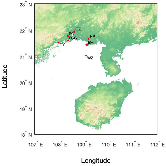
Figure 1.
Location map of the meteorological observation stations in the Beibu Gulf.

Table 1.
Station Locations and Observed Variables.
2.2. Terminology
We adhere to the definitions of ‘fog hour’ and ‘fog day’ as outlined by the China Meteorological Administration (CMA) [32] to identify sea fog occurrence from observations. A ‘fog hour’ is defined as any hour during which the visibility at a given station is less than or equal to 1 and RH is greater than or equal to 90%, under which conditions fog is considered to exist. Liu et al. [33] also adopted this definition. It is important to note that fog hours are specifically associated with fog levels ranging from heavy to very dense (see Table 2). Furthermore, a ‘fog day’ is defined as any day during which a ‘fog hour’ is detected at a station, from 00:00 LT to 23:00 LT, thereby classifying the entire day as a ‘fog day’. Times that do not meet this criterion are labeled as non-fog hours or non-fog days.

Table 2.
Fog weather and associated visibility levels.
The fog and corresponding visibility levels are presented in Table 2. For visibility below 10 , the terminology for fog at different visibility levels follows the definition provided by CMA [32]. Visibility greater than 10 but less than 30 is treated as non-fog conditions in this study (with 30 excluded), indicating that no fog is detected. The upper limit is due to the maximum visibility that the instrument can measure, which is 30 . If visibility exceeds 30 at any given time, it will still be recorded as 30 . Non-fog conditions also require that RH be less than 90% to differ from a fog condition. Furthermore, it should be noted that all instances where rainfall was detected have been removed from the dataset, as precipitation can also affect visibility [18]. This classification ensures that our target is focused on fog occurrence, distinguishing between high visibility in a non-fog condition and low visibility due to fog occurrence rather than precipitation. By training with these filtered instances, the model can better understand the difference between fog and non-fog conditions, thereby providing more accurate predictions of low visibility due to fog.
2.3. Machine Learning (ML) Models
We used three ML models—Random Forest (RF [31]), Extreme Gradient Boosting (XGBoost [29]), and Categorical Boosting (CatBoost [34])—to investigate the visibility of sea fog in the Beibu Gulf. Those models are widely recognized for their effectiveness in predicting fog occurrence and low-visibility conditions [28,30,35,36,37].
We first used regression models to predict visibility. The evaluation of the performance of these models is based on a visibility of less than 10 . The performance of the general models is assessed using Mean Squared Error (MSE), root mean square error (RMSE), mean absolute error (MAE), and the determination coefficient () between predicted visibility and observed visibility on a station-by-station basis. MSE quantifies the average of the squared differences between the predicted visibility and observed visibility, with a lower MSE signifying greater prediction accuracy. When predicting visibility, RMSE provides a more interpretable measure of the magnitude of the prediction error. MAE represents the average of the absolute differences between predicted visibility and observed visibility, indicating the typical prediction error. The determination coefficient () assesses how well the model fits the relationship between observed visibility and predicted visibility. A better fit is typically indicated by a value close to 1. The evaluation parameters align with the methodologies described in Kim et al. [30,38]; the only difference is we adopt MSE rather than bias.
For each model, the training set used sea fog samples collected between 00:00 LT on 1 January 2016, and 23:00 LT on 31 December 2020, comprising 144,716 data points. This dataset includes 41,968 instances of Light Fog, 603 instances of Dense Fog, 591 instances of Severe Dense Fog, 289 instances of Extreme Dense Fog, and 101,265 instances of non-fog conditions, while the testing set used sea fog samples from 00:00 LT on 1 January 2021, to 23:00 LT on 31 December 2021 (25,686 data points). This separation of time ensures that the training and testing sets do not include the same fog events. This separation process has been applied across all models for visibility prediction in the Beibu Gulf. Consequently, models trained using data from 2016 to 2020 are referred to as general models in this work. These general models are then applied to the testing set from 2021, where their performance on visibility is evaluated. It should be noted that all the hyperparameters in the three models have been tuned using GridSearch cross-validation to find the optimal parameters. However, given the current computational resources available to our team, increasing the number of hyperparameters in the testing became infeasible. Therefore, we only tuned max depth, iterations or number of estimators, and learning rate, while keeping other hyperparameters as default, within the limits of our computational capacity.
Table 3 presents the target variable and the features to be used in the ML models. The target variable is visibility, which is influenced by fog occurrence. The features include air temperature (), specific humidity (q), wind speed, wind direction, relative humidity (RH), dew point () and the temperature−dew point difference (). To account for diurnal and seasonal patterns, the month, day, and hour were also included as feature variables. Additionally, considering the coastal region experiences land-sea breezes, wind direction can affect local moisture by carrying water vapor from either the ocean or the land. Therefore, the wind direction and the wind speed will be decomposed into west-east (x-component) and north-south (y-component) components and then applied to ML models.

Table 3.
Target and feature variables for ML models.
Then, the light, heavy, dense, and severe dense fog categories were labeled as ‘0’, ‘1’, ‘2’, and ‘3’, respectively. Predicted visibility outside the ranges specified in Table 2 and under non-fog conditions were labeled as ‘−1’. These labels were used to classify and evaluate the models in terms of accuracy, precision, recall, and F1 score. These metrics evaluate the model’s performance by calculating the number of correctly predicted samples compared to the actual values, which were also adopted in Kim et al. [23] and Wu et al. [39]. Additionally, for better evaluation, predicted visibility values labeled as ‘−1’ are excluded. The formulas for accuracy, precision, recall, and F1 score are given by:
In visibility prediction, True Positive (TP) is the number of predicted samples where sea fog is actually detected, which causes reduced visibility, and the ML models correctly predicted the observed samples. True Negative (TN) is the number of predicted samples where there is no sea fog detected, and the ML models also predicted no sea fog. False Positive (FP) is the number of predicted samples in which there is actually no sea fog, but the ML models incorrectly predicted the presence of sea fog. False Negative (FN) is the number of predicted samples where there is actually sea fog, but it is incorrectly predicted as there is no sea fog.
2.3.1. Random Forest (RF)
RF [31] is a widely used ML algorithm used for both classification and regression tasks [38]. Its ability to efficiently process large datasets makes it particularly useful for visibility predictions [27,28,40,41]. The RF algorithm constructs multiple decision trees and incorporates randomly selected variables at each node to develop regression trees. Each tree within the RF model generates a prediction when predicting target variables. The algorithm then aggregates these individual predictions through either voting (for classification) or averaging (for regression), thereby producing the final predicted values of the target variables. Table 4 presents the parameters for the RF model used for visibility predictions, including the maximum depth and the number of trees, without specifying them for each station. However, using a maximum depth of 9, as adopted in Kim et al. [23], the RF model failed to predict the low visibility samples in our work. By increasing the maximum depth to 20, the RF model successfully made visibility predictions, showing similar results to other models. However, this high maximum depth may lead to overfitting in the RF model, which will be discussed later.

Table 4.
Parameters for Random Forest (RF) model.
2.3.2. Extreme Gradient Boosting (XGBoost)
Similarly to RF, XGBoost [29] is also a decision tree-based machine learning algorithm capable of performing both classification and regression tasks. Based on gradient boosting, XGBoost constructs trees sequentially, with each tree aiming to correct the errors of the previous one. This sequential approach allows for the efficient use of fewer, more optimized trees. Additionally, XGBoost includes built-in features for handling missing values, which enhance its prediction accuracy [42]. This capability is particularly useful for analyzing observational data in regions with limited observations. XGBoost has been widely used to predict visibility [36,37,43]. Table 5 presents the parameters for the XGBoost model used for visibility predictions.

Table 5.
Parameters for the XGBoost model.
2.3.3. Categorical Boosting (CatBoost)
CatBoost [34] is also a gradient enhancement designed for gradient boosting in decision trees [44]. It includes features to prevent overfitting, ensuring robust and reliable performance across various applications, as demonstrated in previous works. For example, Ding et al. [45] applied CatBoost to regenerate satellite aerosol optical depth (AOD) data and estimate gridded PM2.5 from station measurements with AOD and other measurements. Furthermore, Zhang et al. [35] used CatBoost to investigate surface visibility, and Guo et al. [46] used the CatBoost algorithm to accurately predict indoor PM2.5 concentration levels. All of their work demonstrates that CatBoost can accurately predict target variables more effectively than other ML models. Table 6 presents the parameters for the CatBoost model.

Table 6.
Parameters for CatBoost model.
3. Results
Section 3.1 presents the diurnal variations in the frequency of sea fog occurrence and the corresponding atmospheric conditions in the Beibu Gulf. It examines the atmospheric factors influencing the visibility, which are subsequently integrated into ML models. Section 3.2 presents the results of applying the ML models to predict visibility and compares predicted visibility with observed visibility in the Beibu Gulf. Section 3.3 presents the performance evaluation of general models applied to visibility predictions at each observation station.
3.1. Diurnal Variations of Sea Fog
Different atmospheric processes can contribute to the formation of sea fog in the Beibu Gulf. Sea fog occurrence exhibits diurnal variations in the Beibu Gulf. Figure 2 shows the occurrence frequency of sea fog at various LTs. The calculation is based on dividing the total fog hours at each LT by the total occurrences of that specific LT over six years, with data from DX, FC, QZ, and WZ. It is evident that the frequency of the occurrence of sea fog is typically high in the early morning and low in the afternoon, demonstrating a clear diurnal cycle. These diurnal patterns are closely aligned with the findings of Zheng et al. [6], which identify that between 03:00 and 05:00 LT, the highest frequency of sea fog occurrence is observed in the Beibu Gulf. The discussion of these peaks will continue in the following section. Let us focus on sea fog with a visibility range of less than 1 km. As shown in Figure 2, the highest frequency of sea fog occurrence in the Beibu Gulf typically occurs between 04:00 LT and 08:00 LT on a diurnal scale. In particular, QZ, DX and WZ are the three primary locations that exhibit significant diurnal variations in the frequency of sea fog (see Figure 2a,e,f). Particularly between 04:00 LT and 08:00 LT, these stations demonstrate significantly higher occurrence frequencies compared to the other four observation stations. Among these, QZ exhibits the most pronounced variations (see Figure 2a). The high frequency of sea fog observed at these stations can be attributed to their location in areas with a substantial land mass coverage (see Figure 1). Consequently, the surface temperature at these stations would experience more significant changes than at other locations due to the low heat capacity. The air temperature near the surface is significantly affected by changes in surface temperature. Heat and radiation from the surface influence whether the air above reaches the dew point, thus causing the condensation of water vapor and fog occurrence. In contrast, the locations of the stations near or on the ocean typically exhibit the opposite effect. The air near the surface would receive less influence from the surface as the surface temperature would not change significantly due to the large heat capacity of the water.
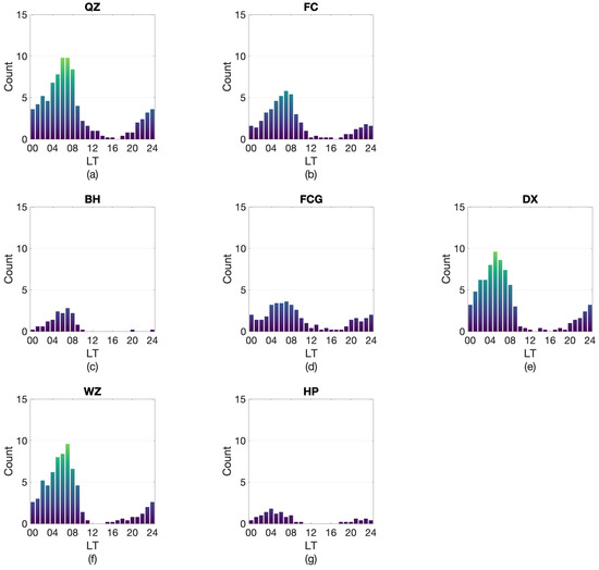
Figure 2.
Six-year average frequency of sea fog occurrence per hour for observation stations: (a) QZ, (b) FC, (c) FCG, (d) DX, (e) BH, (f) WZ, and (g) HP.
Furthermore, when it comes to the fog categories listed in Table 2, their hourly probability histograms are similar across different observation stations (see Figure 3). These histograms almost reach the maximum probability of sea fog occurrence during nighttime and early morning (up to 08:00 LT), while the probability is minimized during the afternoon (see Figure 3a–d. The denser the fog, the higher the likelihood of its occurrence during nighttime, and it is less likely to occur during the daytime, especially in the afternoon (see Figure 3d). A feasible explanation is that the boundary layer and lower atmosphere become more stable after sunset. This stability arises from reduced thermal and radiative effects from the surface, as well as cooling due to longwave radiation emission. As a result, the temperature gradient decreases, leading to a stable temperature stratification in the lower atmosphere. A cooler and more stable atmosphere promotes fog formation. Cooler temperatures enable the air to reach the dew point, thereby increasing RH and saturating water vapor. Stability in the atmosphere means that water vapor is not effectively transported upward, leading to a higher concentration of water vapor near the surface. This excess water vapor will condense when the temperature drops to the dew point. This situation is almost reversed in the afternoon atmosphere, when the boundary layer and lower atmosphere receive substantial thermal and radiative energy from the surface, heating up. The higher temperature increases the capacity of the atmosphere to hold water vapor, causing suspended liquid droplets to undergo evaporation. A warmer surface also triggers convection by heating up the lower atmosphere, which can push water vapor upward and prevent fog formation. Thus, the probability of sea fog occurrence is minimized.
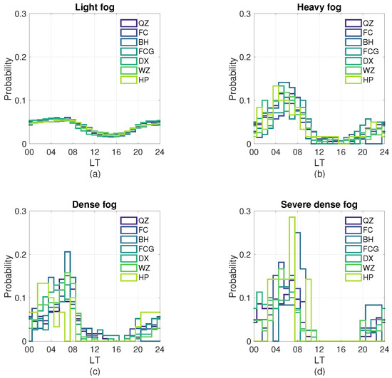
Figure 3.
Hourly probability histograms of different fog categories at Beibu Gulf observation stations in terms of (a) Light Fog, (b) Heavy fog, (c) Dense fog, and (d) Severe dense fog.
The occurrence of sea fog in the Beibu Gulf can be caused by a decrease in air temperature to the dew point. This leads to the saturation of water vapor and subsequent condensation. Figure 4 compares the diurnal variation of atmospheric temperature on days with fog and without fog. Generally, the lower temperature of the day always coincides with a higher frequency of sea fog occurrence, and vice versa (see Figure 2 and Figure 4). The atmospheric temperature on fog days is lower than on non-fog days at all observation stations. In addition, all the stations exhibit lower moisture levels on fog days compared to non-fog days (see Figure 5). This reduction can be attributed to the lower temperatures during fog days, as shown in Figure 4a. The decrease in temperature reaches the dew point, saturating the air, thereby facilitating the condensation of water vapor, which depletes atmospheric moisture. Consequently, the lower moisture levels on fog days are evident in Figure 5a.
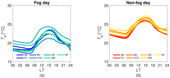
Figure 4.
Six-year average diurnal variation in air temperature on (a) fog and (b) non-fog days at observation stations in the Beibu Gulf.
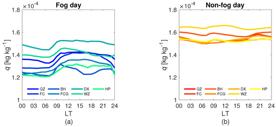
Figure 5.
Six-year average diurnal variation in specific humidity on (a) fog and (b) non-fog days at observation stations in the Beibu Gulf.
The intensity of the wind should be another factor that regulates the occurrence of sea fog in the Beibu Gulf. The lower wind speeds of the day also coincided with a higher frequency of sea fog occurrence, and vice versa (see Figure 6 and Figure 7). Figure 6 and Figure 7 compare the diurnal variations of horizontal wind speed and wind direction on foggy and non-fog days in the Beibu Gulf. It is evident that wind speeds during fog days are lower than those on non-fog days. This is attributed to the fact that low wind speeds in the lower atmosphere weaken convection and the horizontal movement of air, thereby preventing the efficient dispersion of water vapor, which subsequently accumulates water vapor and facilitates fog formation. Additionally, these low wind speeds stabilize the lower atmosphere and reduce turbulence in this region, further aiding in the maintenance of fog. This is evident in HP, which is characterized by lower wind speeds compared to the other six stations. Here, the reduced wind speed allows water vapor to accumulate more easily than at other observation stations. The excess water vapor then condenses to form fog, releasing latent heat that warms the atmosphere. This is in line with Figure 4a and Figure 5a. While other stations have higher wind speeds than HP, fog formation at these stations should not be explained solely by excess water vapor. Considering the lower temperatures compared to non-fog days (see Figure 4a), these stations should be more regularly influenced by decreases in temperature, either through the radiative cooling of moist air or the frontal lifting of warmer air.
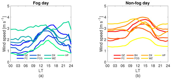
Figure 6.
Six-year average diurnal variation in wind speeds on (a) fog and (b) non-fog days at observation stations in the Beibu Gulf.
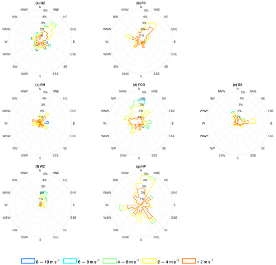
Figure 7.
Wind direction frequency for different wind speeds during fog hours at observation stations in the Beibu Gulf.
Furthermore, in addition to the fog hours when the wind is calm and has a low speed, the wind direction should also be of concern. Figure 7 shows that when visibility is below 1 , the Beibu Gulf is predominantly influenced by north and northeast winds, with a typical wind direction between 0° and 45°. Considering the locations of each station, the north and northeast winds could be associated with the land breeze, which typically forms during the nighttime due to a decrease in surface and air temperature along the coast. This cooler air then advects toward the sea, mixing with the air over the ocean, which can further decrease the temperature and increase the atmospheric RH over the sea area. This process can lead to the condensation of water vapor, fog formation, and subsequently, a decrease in visibility. This low visibility and low temperature can be identified in Figure 3 and Figure 4, where the lowest values consistently occur during nighttime. This suggests that, apart from wind speed, wind direction should also be considered as a factor in determining sea fog occurrence and, consequently, visibility.
Therefore, the differences in atmospheric conditions between fog and non-fog days suggest that the frequency of sea fog occurrence in the Beibu Gulf depends on location and is highly influenced by changes in atmospheric temperature, specific humidity, wind speed, and wind direction. These factors eventually contribute to changes in RH of the lower atmosphere, thus facilitating the condensation of water vapor and, consequently, fog formation. These variables, along with the month, day, and hour, will be used as feature variables in the RF, XGBoost, and CatBoost models to predict visibility. It is important to note that the wind at 0° and 360° indicates the same wind direction, which is from the north. Therefore, wind, as one of the feature variables that can affect the occurrence of sea fog, will be decomposed into west-east (x-component) and north-south (y-component) components. This decomposition will be applied to wind speed, as presented in Table 3, and subsequently used in the ML models.
3.2. Model Analysis: General Predications
The outputs of all ML models are visualized using scatter density plots, comparing predicted visibility against observed visibility (Figure 8a for RF, Figure 8b for XGBoost and Figure 8c for CatBoost). The color gradient represents the density of points in a given area of the prediction-observation plots using Gaussian kernel density estimation. Figure 8 shows that the three models—RF, XGBoost, and CatBoost—present different visibility predictions across the Beibu Gulf. The scatter points are concentrated within the predicted range of 4 to 8 for RF, 2 to 10 for XGBoost, and 3 to 8 for CatBoost.

Figure 8.
Performance comparison of predictive visibility and observed visibility of general (a) RF, (b) XGBoost, and (c) CatBoost models.
These general ML models were trained using atmospheric variables corresponding to visibility ranges from 0 to 30 . Therefore, the performance metrics are for the entire visibility range rather than just those below 10 . The metrics evaluating performance are presented in Table 7. All three general models show good performance but with varying values. The RF model exhibited an MSE of km2, an RMSE of , an MAE of , and an of 0.88. The RF model also showed an accuracy of 0.98, a precision of 0.96, a recall of 0.98, and an F1 score of 0.97. In contrast, XGBoost demonstrated a higher MSE of km2, an RMSE of , and an MAE of , with an of 0.72, indicating a slightly lower accuracy than RF for the prediction of visibility. However, XGBoost still performed well, with an accuracy of 0.98, a precision of 0.98, a recall of 0.98, and an F1 score of 0.98. Finally, CatBoost demonstrated competitive performance with an MSE of km2, an RMSE of , and an MAE of . Its value was 0.84, slightly lower than that of RF but higher than that of XGBoost. CatBoost achieved an accuracy of 0.98, a precision of 0.95, a recall of 0.98, and an F1 score of 0.97.

Table 7.
Performance metrics for different models.
The performance of RF, particularly its accuracy and other classification metrics, indicates strong predictive capabilities. Although XGBoost has a slightly lower compared to the other models and performs slightly lower in some metrics, it still demonstrates competitive results.
RF accurately predicted the observed visibility below 10 km, closely aligned with the line y = x. However, within the low visibility range (<4 km), RF appears to slightly overestimate (see Figure 8a). XGBoost and CatBoost show similar visibility predictions (see Figure 8b,c), with a similar distribution of those scatter points. In addition, RF and CatBoost do not perform well in predicting low visibility, (see Figure 8a,c). This limitation has also been identified in Kim et al. [38]. We assume that this is due to the extremely limited number of dense and severe dense fog samples, as the sample size can significantly impact model performance [47]. As a result, the RF and the other models cannot satisfactorily capture the feature of low-visibility samples due to dense or severe-dense fog. This eventually leads to unsatisfactory performance in predicting low visibility. Long-term observation of low visibility due to dense and severe-dense fog occurrence is required. In contrast, XGBoost effectively captures most low visibility ranges. Although XGBoost shows a smaller , it aligns well with observations within the lower visibility range of less than 4 km (see Figure 8b).
It is important to note that the values for the training set are close to those of the testing set, whether it is for RF, XGBoost, or CatBoost. This suggests that overfitting during model training is weak or almost nonexistent. Particularly for RF and CatBoost, the difference in between the training set and the testing set is very small (0.92 for training and 0.88 for testing in RF; 0.86 for training and 0.84 for testing in CatBoost), indicating that these models can generalize well to unseen data and provide satisfactory performance. In contrast, for XGBoost, the for the training set is 0.70, while it is 0.72 for the testing set, suggesting that overfitting is almost absent. However, given the relatively low , additional feature variables may be needed for future training to improve performance.
3.3. Model Analysis: Station-Based Predictions
Applying the general models to each observation station to predict visibility in 2021, the performance of the visibility prediction varied across the stations. For RF, the best performance can be observed in FC (Figure 9b), BH (Figure 9c), FCG (Figure 9d), DX (Figure 9e) and HP (Figure 9g), with the scatter points more concentrated and closer to the line y = x. This pattern is similar to the results from the general XGBoost and CatBoost models for the same stations, but the distribution of scatter points is less pronounced compared to RF (see Figure 10b for FC using XGBoost, and Figure 11b for FC using CatBoost; see Figure 10c for BH using XGBoost, and Figure 11c for BH using CatBoost; see Figure 10d for FCG using XGBoost, and Figure 11d for FCG using CatBoost; see Figure 10e for DX using XGBoost, and Figure 11e for DX using CatBoost; see Figure 10g for HP using XGBoost, and Figure 11g for HP using CatBoost).
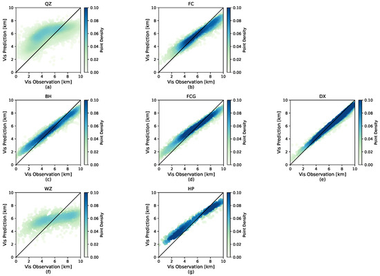
Figure 9.
Performance of General RF models: predicted visibility vs. observed visibility for (a) QZ, (b) FC, (c) FCG, (d) DX, (e) BH, (f) WZ, and (g) HP.
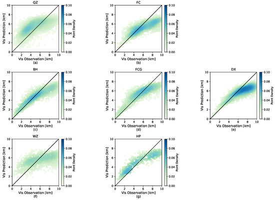
Figure 10.
Performance of the general XGBoost model: predicted visibility vs. observed visibility for (a) QZ, (b) FC, (c) FCG, (d) DX, (e) BH, (f) WZ, and (g) HP.
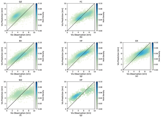
Figure 11.
Performance of CatBoost models: predicted visibility vs. observed visibility for (a) QZ, (b) FC, (c) FCG, (d) DX, (e) BH, (f) WZ, and (g) HP.
For the remaining stations, the situation becomes slightly different. The concentration is less significant as observed at the QZ and WZ stations. The weaker concentration among these stations—QZ and WZ—suggests that the performance of the general models at these locations is not as robust as at FC, BH, FCG, DX, and HP (see Figure 9b for FC using RF, Figure 10b for FC using XGBoost, and Figure 11b for FC using CatBoost; see Figure 9c for BH using RF, Figure 10c for BH using XGBoost, and Figure 11c for BH using CatBoost; see Figure 9d for FCG using RF, Figure 10d for FCG using XGBoost, and Figure 11d for FCG using CatBoost; see Figure 9e for DX using RF, Figure 10e for DX using XGBoost, and Figure 11e for DX using CatBoost; see Figure 9g for HP using RF, Figure 10g for HP using XGBoost, and Figure 11g for HP using CatBoost). Given that QZ is an inland station and WZ is located far from land (see Figure 1), while the majority of the training data comes from coastal regions, the model performs better at stations like FC, BH, FCG, DX, and HP. To enhance the model performance in the future, it would be beneficial to include location-specific information, particularly geographical or topographical variables, in the future training process.
Table 8 shows the performance metrics for RF models in predicting visibility at various observation stations within the Beibu Gulf. The QZ station has an MSE of km2, an RMSE of , an MAE of , and an of 0.70, indicating relatively robust model performance. The FC station shows an MSE of km2, an RMSE of , an MAE of , and an of 0.92, reflecting a strong predictive capacity. Similarly, the BH station demonstrates solid performance with an MSE of km2, an RMSE of , an MAE of , and an of 0.90. The FCG station exhibits an MSE of km2, an RMSE of , an MAE of , and an of 0.93, indicating strong model performance. The DX station, with an MSE of km2, an RMSE of , an MAE of , and an of 0.96, shows the best performance among all stations. In contrast, the WZ station has an MSE of km2, an RMSE of , an MAE of , and an of 0.66, reflecting moderate performance. Lastly, the HP station reveals an MSE of km2, an RMSE of , an MAE of , and an of 0.86, indicating strong model performance.

Table 8.
Performance metrics of the general RF model at seven observation stations.
Overall, both the XGBoost and CatBoost models demonstrate effective predictive capabilities for visibility due to fog in the Beibu Gulf, particularly at coastal stations such as FC, BH, FCG, and DX, where their performance is strong, similar to the RF model. However, the metrics indicate that their performance is somewhat lower than that of the RF model. The models also perform more moderately at the inland station QZ and at the WZ station, which is located on an island far from the mainland. These variations in model performance across different locations suggest that while both XGBoost and CatBoost are generally effective, their accuracy may also be influenced by the geographic or topographical characteristics of the observation stations.
Table 9 presents the performance metrics for the XGBoost models in predicting visibility at observation stations in the Beibu Gulf. At the QZ station, the model exhibits relatively good performance, with an MSE of km2, an RMSE of , an MAE of , and an of 0.73. The FC station shows even stronger performance, with an MSE of km2, an RMSE of , an MAE of , and an of 0.75. Similarly, the BH station performs satisfactorily, with an MSE of km2, an RMSE of , an MAE of , and an of 0.68. The FCG station also demonstrates good performance, with an MSE of km2, an RMSE of , an MAE of , and an of 0.71. Notably, the DX station achieves strong results, with an MSE of km2, an RMSE of , an MAE of , and an of 0.76. On the other hand, the WZ station reflects more moderate performance, with an MSE of km2, an RMSE of , an MAE of , and an of 0.63. Lastly, the HP station, with an MSE of km2, an RMSE of , an MAE of , and an of 0.57, also demonstrates moderate accuracy.

Table 9.
Performance metrics of the general XGBoost model at seven observation stations.
Table 10 presents the performance metrics for the CatBoost models in predicting visibility at observation stations in the Beibu Gulf. At the QZ station, the model exhibits moderate performance, with an MSE of km2, an RMSE of , an MAE of , and an of 0.68. The FC station shows stronger performance, with an MSE of km2, an RMSE of , an MAE of , and an of 0.87. Similarly, the BH station performs well, with an MSE of km2, an RMSE of , an MAE of , and an of 0.86. The FCG station also demonstrates satisfactory performance, with an MSE of km2, an RMSE of , an MAE of , and an of 0.86. Notably, the DX station achieves the strongest results, with an MSE of km2, an RMSE of , an MAE of , and an of 0.92. On the other hand, the WZ station reflects more moderate performance, with an MSE of km2, an RMSE of , an MAE of , and an of 0.65. Lastly, the HP station, with an MSE of km2, an RMSE of , an MAE of , and an of 0.80, also demonstrates good model performance.

Table 10.
Performance metrics of the general CatBoost model at seven observation stations.
4. Discussion
These general ML models were trained using atmospheric variables corresponding to visibility ranges from 0 to 30 . Therefore, the performance metrics reflect the entire visibility range rather than just those below 10 . The metrics evaluating the performance of these general models are presented in Table 7. All three models demonstrate distinct performance levels, with values ranging from 0.72 to 0.88. The RF model demonstrated strong performance, with an MSE of km2, an RMSE of , an MAE of , and an of 0.88. The RF model’s high classification metrics, including an accuracy of 0.98, a precision of 0.96, a recall of 0.98, and an F1 score of 0.97, underscore its predictive capabilities. However, the model’s complexity, particularly its depth, raises concerns about potential overfitting, as it may capture noise rather than generalize well to new data.
In contrast, the XGBoost model showed a higher MSE of km2, an RMSE of , and an MAE of , with an of 0.72. While XGBoost’s and error metrics suggest it is less accurate than RF, it maintains robust classification capabilities, with an accuracy, precision, recall, and F1 score all at 0.98. XGBoost effectively balances model complexity with predictive power, handling a variety of data patterns.
CatBoost also performed competitively, with an MSE of km2, an RMSE of , and an MAE of . Its of 0.84 indicates a balance between RF and XGBoost in terms of accuracy and complexity. CatBoost’s classification metrics, with an accuracy of 0.98, a precision of 0.95, a recall of 0.98, and an F1 score of 0.97, reflect its strong performance and reduced risk of overfitting compared to RF.
Our study primarily evaluates model performance for visibility below 10 . However, the number of data points with visibility below 10 is lower than those with visibility between 10 and 30 . Since the models were trained on the full visibility range but evaluated primarily on visibility below 10 , this imbalance may lead to an overestimation of visibility in the lower range. Nevertheless, including visibility data up to 30 aligns with our goal of providing accurate predictions for low visibility due to fog, capturing the transition from non-fog to fog conditions. This outcome is a necessary consequence of our approach.
Furthermore, the RMSE values observed in the models, such as for XGBoost or other similar values, while indicative of strong performance, can still be significant when predicting fog occurrence, particularly concerning the management of maritime safety and activities. To potentially reduce these errors, future efforts could focus on incorporating more localized and high-resolution data, such as real-time observations from ground-based sensors, and enhancing model inputs by considering additional meteorological variables (e.g., vertical temperature profiles, surface thermal energy transfer, wind shear, and topography). However, these variables are not available in the current dataset, so there is still room for improvement, though it cannot be addressed at this moment. Further observations and efforts will be needed.
The performance of these models, particularly RF and CatBoost, is less effective in predicting low visibility (see Figure 8a for RF and Figure 8c for CatBoost). This limitation, also noted by Kim et al. [38], is likely due to the limited number of dense and severe fog samples available for training. Consequently, these models struggle to capture the characteristics of low-visibility conditions, leading to less satisfactory predictions. However, XGBoost has demonstrated a better capability to predict lower visibility associated with sea fog occurrence in the Beibu Gulf, which can be attributed to its ability to handle diverse data patterns more effectively and its balance between complexity and accuracy.
Since the models were not trained with geographical or topographical variables, this may explain discrepancies in visibility prediction performance. For instance, QZ is a more inland location compared to other stations, while WZ is situated far from land. These geographical differences, as observed on the map, likely influence model performance. Given the limitations of our current dataset, future work should incorporate geographical or topographical variables into model training to improve prediction accuracy, thereby addressing these discrepancies more robustly.
5. Conclusions
Sea fog occurs frequently during the nighttime in the Beibu Gulf, which can be attributed to lower temperatures and decreased wind speeds during the night. These conditions increase the relative humidity of the atmosphere, facilitating the condensation of water vapor and thus fog formation. During the daytime, rising air temperatures increase the saturation vapor pressure, leading to the evaporation of suspended liquid droplets and, consequently, the dissipation of fog. As a result, the frequency of sea fog occurrence is minimized during the daytime.
The observed atmospheric conditions, along with the specific month, day, and hour variables, were utilized as features for predicting visibility due to fog occurrence using machine learning (ML) models. This study employed three typical ML models—Random Forest (RF), Extreme Gradient Boosting (XGBoost), and Categorical Boosting (CatBoost)—to predict the visibility of sea fog in the Beibu Gulf. The results suggest that ML models can effectively predict visibility in this region. The models were trained using five years of observational data (2016 to 2020) from seven observation stations in the Beibu Gulf—Qinzhou (QZ), Fangcheng (FC), Beihai (BH), Fangchenggang (FCG), Dongxing (DX), Weizhou Island (WZ), and Hepu (HP)—and tested using observational data from 2021. The results indicate that XGBoost has demonstrated a better capability to predict the lower visibility associated with sea fog occurrence in the Beibu Gulf, outperforming RF and CatBoost in predicting low-visibility events. Future studies focusing on regional or local low-visibility events due to fog occurrence could consider utilizing ML models, especially XGBoost.
However, although all the ML models applied in this work show satisfactory performance in predicting the visibility caused by the occurrence of sea fog, the observed limitations related to geographical and topographical differences must be carefully considered. In this work, QZ is a station located inland, whereas WZ is situated over the ocean and far from land. Their distinct geographical locations and topographical characteristics may affect the models’ performance when using data collected from these two sites. The models cannot accurately predict visibility at these two stations, showing relatively weak performance compared to the other five stations. Therefore, incorporating geographical and topographical variables into model training should help improve the accuracy of visibility predictions related to sea fog.
Author Contributions
Conceptualization, Q.H. and J.L.; methodology, J.L.; software, Q.H.; validation, Q.H. and J.L.; formal analysis, Q.H.; investigation, P.Z. and X.G.; resources, P.Z. and X.G.; data curation, P.Z. and X.G.; writing—original draft preparation, Q.H.; writing—review and editing, Q.H. and J.L.; visualization, Q.H.; supervision, P.Z., X.G. and J.L.; project administration, P.Z.; funding acquisition, P.Z. and X.G. All authors have read and agreed to the published version of the manuscript.
Funding
This research was funded by Guangxi Transportation (Railway) Intelligent Integrated Service Technology—Technical Research on Meteorological Risk Warning Model for Guangxi Railway System (grant number 2022ZL07), the Guangxi Key Research and Development Program (grant number AB20159013), and the National Natural Science Foundation of China (grant number 41675136).
Data Availability Statement
The data used in this study are not publicly available due to privacy. However, they may be available from the corresponding author upon reasonable request and with permission from the relevant authorities.
Acknowledgments
The authors gratefully acknowledge Hao Chen from the Department of Statistics, University of Auckland, for providing technical support in using machine learning models.
Conflicts of Interest
The authors Peng Zeng and Xiaowei Guo were employed by the company Guangxi Meteorological Disaster Prevention Center; they have no conflicts of interest. The remaining authors declare that the research was conducted in the absence of any commercial or financial relationships that could be construed as a potential conflict of interest.
Abbreviations
The following abbreviations are used in this manuscript:
| QZ | Qinzhou |
| FC | Fangcheng |
| BH | Beihai |
| FCG | Fangchenggang |
| DX | Dongxing |
| WZ | Weizhou Island |
| HP | Hepu |
| RH | Relative Humidity |
| Air Temperature | |
| Dew point Temperature | |
| q | Specific Humidity |
| vis | Visibility |
| LT | Local Time |
| AWS | Automated Weather Stations |
| MSE | Mean Squared Error |
| MAE | Mean Absolute Error |
| RMSE | Root Mean Squared Error |
| TP | True Positive |
| TN | True Negative |
| FP | False Positive |
| FN | False Negative |
| RF | Random Forest |
| XGBoost | Extreme Gradient Boosting |
| CatBoost | Categorical Boosting |
| CMA | China Meteorological Administration |
| ML | Machine Learning |
| NWP | Numerical Weather Prediction |
| GRAPES | Global and Regional Assimilation and Prediction System |
| AOD | Aerosol Optical Depth |
References
- Koračín, D.; Dorman, C.E.; Lewis, J.M.; Hudson, J.G.; Wilcox, E.M.; Torregrosa, A. Marine fog: A review. Atmos. Res. 2014, 143, 142–175. [Google Scholar] [CrossRef]
- Gultepe, I.; Milbrandt, J.A.; Zhou, B. Marine fog: A review on microphysics and visibility prediction. In Marine Fog: Challenges and Advancements in Observations, Modeling, and Forecasting; Springer: Cham, Switzerland, 2017; pp. 345–394. [Google Scholar]
- Liu, K.; Yu, Q.; Yuan, Z.; Yang, Z.; Shu, Y. A systematic analysis for maritime accidents causation in Chinese coastal waters using machine learning approaches. Ocean Coast. Manag. 2021, 213, 105859. [Google Scholar] [CrossRef]
- Zhang, Z.; Zhang, X.; Xu, Z.; Yao, H.; Li, G.; Liu, X. Emergency countermeasures against marine disasters in Qingdao City on the basis of scenario analysis. Nat. Hazards 2015, 75, 233–255. [Google Scholar] [CrossRef]
- Yuan, X.; Tipparat, P.; Zhang, Z.; Jing, X.; Ming, J. Fishery and Aquaculture Insurance in China; FAO Fisheries and Aquaculture Circular; FAO: Rome, Italy, 2017; p. C1139. [Google Scholar]
- Zheng, F.; Luo, X.; Zhong, L.; Wei, J. Preliminary analysis of sea fog characteristics over Beibu Gulf area. J. Appl. Oceanogr. 2021, 40, 324–331. [Google Scholar]
- Qu, F.; Liu, S.; Yi, Y.; Huang, J. The observation and analysis of a sea fog event in South China. J. Trop. Meteorol. 2008, 24, 490–496. [Google Scholar]
- Kong, X.; Jiang, Z.; Ma, M.; Chen, N.; Chen, J.; Shen, X.; Bai, C. The spatiotemporal distribution of sea fog in offshore of China based on FY-4A satellite data. J. Phys. Conf. Ser. 2023, 2486, 012015. [Google Scholar] [CrossRef]
- Huang, H.; Huang, B.; Yi, L.; Liu, C.; Tu, J.; Wen, G.; Mao, W. Evaluation of the global and regional assimilation and prediction system for predicting sea fog over the South China Sea. Adv. Atmos. Sci. 2019, 36, 623–642. [Google Scholar] [CrossRef]
- Han, L.; Long, J.; Xu, F.; Xu, J. Decadal shift in sea fog frequency over the northern South China Sea in spring: Interdecadal variation and impact of the Pacific Decadal Oscillation. Atmos. Res. 2022, 265, 105905. [Google Scholar] [CrossRef]
- Ellrod, G.P. Advances in the detection and analysis of fog at night using GOES multispectral infrared imagery. Weather Forecast. 1995, 10, 606–619. [Google Scholar] [CrossRef]
- Gao, S.; Wu, W.; Zhu, L.; Fu, G. Detection of nighttime sea fog/stratus over the Huang-hai Sea using MTSAT-1R IR data. Acta Oceanol. Sin. 2009, 28, 23–35. [Google Scholar]
- Wu, X.; Li, S. Automatic sea fog detection over Chinese adjacent oceans using Terra/MODIS data. Int. J. Remote Sens. 2014, 35, 7430–7457. [Google Scholar] [CrossRef]
- Ahn, M.-H.; Sohn, E.-H.; Hwang, B.-J. A new algorithm for sea fog/stratus detection using GMS-5 IR data. Adv. Atmos. Sci. 2003, 20, 899–913. [Google Scholar] [CrossRef]
- Xiao, Y.-F.; Zhang, J.; Qin, P. An algorithm for daytime sea fog detection over the Greenland Sea based on MODIS and CALIOP data. J. Coast. Res. 2019, 90, 95–103. [Google Scholar] [CrossRef]
- Heo, K.-Y.; Park, S.; Ha, K.-J.; Shim, J.-S. Algorithm for sea fog monitoring with the use of information technologies. Meteorol. Appl. 2014, 21, 350–359. [Google Scholar] [CrossRef]
- Fu, G.; Li, P.; Crompton, J.G.; Guo, J.; Gao, S.; Zhang, S. An observational and modeling study of a sea fog event over the Yellow Sea on 1 August 2003. Meteorol. Atmos. Phys. 2010, 107, 149–159. [Google Scholar] [CrossRef]
- Gultepe, I.; Milbrandt, J.A. Probabilistic parameterizations of visibility using observations of rain precipitation rate, relative humidity, and visibility. J. Appl. Meteorol. Climatol. 2010, 49, 36–46. [Google Scholar] [CrossRef]
- Román-Cascón, C.; Steeneveld, G.J.; Yagüe, C.; Sastre, M.; Arrillaga, J.A.; Maqueda, G. Forecasting radiation fog at climatologically contrasting stations: Evaluation of statistical methods and WRF. Q. J. R. Meteorol. Soc. 2016, 142, 1048–1063. [Google Scholar] [CrossRef]
- da Rocha, R.P.; Gonçalves, F.L.T.; Segalin, B. Fog events and local atmospheric features simulated by regional climate model for the metropolitan area of São Paulo, Brazil. Atmos. Res. 2015, 151, 176–188. [Google Scholar] [CrossRef]
- Román-Cascón, C.; Yagüe, C.; Steeneveld, G.-J.; Morales, G.; Arrillaga, J.A.; Sastre, M.; Maqueda, G. Radiation and cloud-base lowering fog events: Observational analysis and evaluation of WRF and HARMONIE. Atmos. Res. 2019, 229, 190–207. [Google Scholar] [CrossRef]
- Han, J.H.; Kim, K.J.; Joo, H.S.; Han, Y.H.; Kim, Y.T.; Kwon, S.J. Sea fog dissipation prediction in Incheon Port and Haeundae Beach using machine learning and deep learning. Sensors 2021, 21, 5232. [Google Scholar] [CrossRef]
- Kim, J.; Kim, S.H.; Seo, H.W.; Wang, Y.V.; Lee, Y.G. Meteorological characteristics of fog events in Korean smart cities and machine learning based visibility estimation. Atmos. Res. 2022, 275, 106239. [Google Scholar] [CrossRef]
- Guo, X.; Wan, J.; Liu, S.; Xu, M.; Sheng, H.; Yasir, M. A scse-linknet deep learning model for daytime sea fog detection. Remote Sens. 2021, 13, 5163. [Google Scholar] [CrossRef]
- Wang, Y.; Qiu, Z.; Zhao, D.; Ali, M.A.; Hu, C.; Zhang, Y.; Liao, K. Automatic detection of daytime sea fog based on supervised classification techniques for fy-3d satellite. Remote Sens. 2023, 15, 2283. [Google Scholar] [CrossRef]
- Cornejo-Bueno, S.; Casillas-Pérez, D.; Cornejo-Bueno, L.; Chidean, M.I.; Caamaño, A.J.; Cerro-Prada, E.; Casanova-Mateo, C.; Salcedo-Sanz, S. Statistical analysis and machine learning prediction of fog-caused low-visibility events at A-8 motor-road in Spain. Atmosphere 2021, 12, 679. [Google Scholar] [CrossRef]
- Dewi, R.; Harsa, H. Fog prediction using artificial intelligence: A case study in Wamena Airport. J. Phys. Conf. Ser. 2020, 1528, 012021. [Google Scholar] [CrossRef]
- Kim, B.-Y.; Cha, J.W.; Chang, K.-H.; Lee, C. Visibility prediction over South Korea based on random forest. Atmosphere 2021, 12, 552. [Google Scholar] [CrossRef]
- Chen, T.; Guestrin, C. XGBoost: A Scalable Tree Boosting System. In Proceedings of the ACM SIGKDD International Conference on Knowledge Discovery and Data Mining, San Francisco, CA, USA, 13–17 August 2016; pp. 785–794. [Google Scholar] [CrossRef]
- Kim, B.-Y.; Belorid, M.; Cha, J.W. Short-term visibility prediction using tree-based machine learning algorithms and numerical weather prediction data. Weather Forecast. 2022, 37, 2263–2274. [Google Scholar] [CrossRef]
- Breiman, L. Random Forests. Mach. Learn. 2001, 45, 5–32. [Google Scholar] [CrossRef]
- China Meteorological Administration. Surface Meteorological Observation Standards; China Meteorological Press: Beijing, China, 2003. [Google Scholar]
- Liu, W.; Han, Y.; Li, J.; Tian, X.; Liu, Y. Factors affecting relative humidity and its relationship with the long-term variation of fog-haze events in the Yangtze River Delta. Atmos. Environ. 2018, 193, 242–250. [Google Scholar] [CrossRef]
- Friedman, J.H. Greedy Function Approximation: A Gradient Boosting Machine. Ann. Stat. 2001, 29, 1189–1232. [Google Scholar] [CrossRef]
- Zhang, X.; Gui, K.; Zeng, Z.; Fei, Y.; Li, L.; Zheng, Y.; Peng, Y.; Liu, Y.; Shang, N.; Zhao, H.; et al. Mapping the seamless hourly surface visibility in China: A real-time retrieval framework using a machine-learning-based stacked ensemble model. Npj Clim. Atmos. Sci. 2024, 7, 68. [Google Scholar] [CrossRef]
- Zhen, M.; Yi, M.; Luo, T.; Wang, F.; Yang, K.; Ma, X.; Cui, S.; Li, X. Application of a Fusion Model Based on Machine Learning in Visibility Prediction. Remote Sens. 2023, 15, 1450. [Google Scholar] [CrossRef]
- Yu, Z.; Qu, Y.; Wang, Y.; Ma, J.; Cao, Y. Application of machine-learning-based fusion model in visibility forecast: A case study of Shanghai, China. Remote Sens. 2021, 13, 2096. [Google Scholar] [CrossRef]
- Kim, B.-Y.; Cha, J.W.; Chang, K.-H.; Lee, C. Estimation of the visibility in Seoul, South Korea, based on particulate matter and weather data, using machine-learning algorithm. Aerosol Air Qual. Res. 2022, 22, 220125. [Google Scholar] [CrossRef]
- Wu, Z.; Wu, F.; Chai, J.; Zhan, C.; Yu, Z. Prediction of daily precipitation based on deep learning and broad learning techniques. In Proceedings of the 2019 IEEE 14th International Conference on Intelligent Systems and Knowledge Engineering (ISKE), Dalian, China, 14–16 November 2019; pp. 513–519. [Google Scholar]
- Peláez-Rodríguez, C.; Pérez-Aracil, J.; Casanova-Mateo, C.; Salcedo-Sanz, S. Efficient prediction of fog-related low-visibility events with Machine Learning and evolutionary algorithms. Atmos. Res. 2023, 295, 106991. [Google Scholar] [CrossRef]
- Alhathloul, S.H.; Mishra, A.K.; Khan, A.A. Low visibility event prediction using random forest and K-nearest neighbor methods. Theor. Appl. Climatol. 2024, 155, 1289–1300. [Google Scholar] [CrossRef]
- Aydin, Z.E.; Ozturk, Z.K. Performance analysis of XGBoost classifier with missing data. Manch. J. Artif. Intell. Appl. Sci. (MJAIAS) 2021, 2, 2021. [Google Scholar]
- Peng, X.; Xie, T.-T.; Tang, M.-X.; Cheng, Y.; Peng, Y.; Wei, F.-H.; Cao, L.-M.; Yu, K.; Du, K.; He, L.-Y.; et al. Critical role of secondary organic aerosol in urban atmospheric visibility improvement identified by machine learning. Environ. Sci. Technol. Lett. 2023, 10, 976–982. [Google Scholar] [CrossRef]
- Dorogush, A.V.; Ershov, V.; Gulin, A. CatBoost: Gradient boosting with categorical features support. arXiv 2018, arXiv:1810.11363. [Google Scholar]
- Ding, Y.; Chen, Z.; Lu, W.; Wang, X. A CatBoost approach with wavelet decomposition to improve satellite-derived high-resolution PM2.5 estimates in Beijing-Tianjin-Hebei. Atmos. Environ. 2021, 249, 118212. [Google Scholar] [CrossRef]
- Guo, Z.; Wang, X.; Ge, L. Classification prediction model of indoor PM2. 5 concentration using CatBoost algorithm. Front. Built Environ. 2023, 9, 1207193. [Google Scholar] [CrossRef]
- Schütz, M.; Schütz, A.; Bendix, J.; Thies, B. Improving Classification-based Nowcasting of Radiation Fog with Machine Learning based on Filtered and Preprocessed Temporal Data. Q. J. R. Meteorol. Soc. 2024, 150, 577–596. [Google Scholar] [CrossRef]
Disclaimer/Publisher’s Note: The statements, opinions and data contained in all publications are solely those of the individual author(s) and contributor(s) and not of MDPI and/or the editor(s). MDPI and/or the editor(s) disclaim responsibility for any injury to people or property resulting from any ideas, methods, instructions or products referred to in the content. |
© 2024 by the authors. Licensee MDPI, Basel, Switzerland. This article is an open access article distributed under the terms and conditions of the Creative Commons Attribution (CC BY) license (https://creativecommons.org/licenses/by/4.0/).