Abstract
By utilizing top-of-atmosphere radiation (TOAR) data from China’s new generation of geostationary satellites (FY-4A and FY-4B) along with interpretable machine learning models, near-surface particulate matter concentrations in China were estimated, achieving hourly temporal resolution, 4 km spatial resolution, and 100% spatial coverage. First, the cloudless TOAR data were matched and modeled with the solar radiation products from the ERA5 dataset to construct and estimate a fully covered TOAR dataset under assumed clear-sky conditions, which increased coverage from 20–30% to 100%. Subsequently, this dataset was applied to estimate particulate matter. The analysis demonstrated that the fully covered TOAR dataset (R2 = 0.83) performed better than the original cloudless dataset (R2 = 0.76). Additionally, using feature importance scores and SHAP values, the impact of meteorological factors and air mass trajectories on the increase in PM10 and PM2.5 during dust events were investigated. The analysis of haze events indicated that the main meteorological factors driving changes in particulate matter included air pressure, temperature, and boundary layer height. The particulate matter concentration products obtained using fully covered TOAR data exhibit high coverage and high spatiotemporal resolution. Combined with data-driven interpretable machine learning, they can effectively reveal the influencing factors of particulate matter in China.
1. Introduction
PM10 and PM2.5, which are atmospheric particulate matter with aerodynamic diameters less than 10 μm and 2.5 μm, respectively, are significant atmospheric pollutants that have garnered widespread attention [1,2,3]. China has led to increased particulate matter pollution, posing significant threats to public health and safety [4]. Numerous studies have indicated that prolonged exposure to particulate matter pollution can lead to cardiovascular and respiratory diseases, ultimately resulting in premature death [5,6,7,8]. Moreover, increasingly severe wildfires have contributed to significant particulate matter pollution [9]. Thus, investigating the causes, progression, and distribution characteristics of particulate matter pollution is crucial for mitigating its adverse effects [10,11]. With the implementation of stricter air quality management policies, there is an urgent need for detailed distribution data on particulate matter. Accurately obtaining particulate matter concentrations with broader spatial coverage and higher spatiotemporal resolution is essential for addressing scientific issues and developing effective environmental policies [12,13].
Aerosol optical depth (AOD) derived from satellites exhibits a strong correlation with particulate matter and can be utilized to estimate particulate matter concentrations [14,15]. Previous studies have successfully utilized AOD products from polar-orbiting satellite sensors, such as MODIS, VIIRS, MISR, and CALIPSO, to obtain near-surface particulate matter concentration products [16,17,18,19,20,21]. However, polar-orbiting satellite data products have lower temporal resolution, which hampers continuous observations of particulate matter concentrations and limits their application in air pollution research. To achieve high spatiotemporal resolution in particulate matter data, geostationary satellite data products, with temporal resolutions of up to 10–15 min, have been employed for estimating particulate matter concentrations. Examples include the Geostationary Ocean Color Imager (GOCI) on the Communication, Ocean, and Meteorological Satellite (COMS) and the Geostationary Environment Monitoring Spectrometer (GEMS) from South Korea; the Advanced Himawari Imager (AHI) on Japan’s Himawari-8 geostationary satellite; the Advanced Baseline Imager (ABI) on the United States’ GOES-16 geostationary satellite; and TEMPO instrument operated by the United States [22,23,24,25,26,27]. However, the observation range of these sensors is inadequate for covering the entirety of China. It was not until 11 December 2016 that China launched the new-generation geostationary meteorological satellite FY-4A, resolving the issue of inadequate coverage by geostationary satellite observations in China. This satellite provided the data foundation for obtaining particulate matter concentration products covering the entire territory of China [28].
Although AOD products provide broader coverage, their spatial applicability is often restricted due to interference from clouds or bright surfaces [29,30]. Consequently, some researchers have proposed using satellite top-of-atmosphere reflectance (TOAR) data directly for particulate matter estimation, which has shown promising results. For example, Liu, et al. [31] and Wang, et al. [32] utilized TOAR data from the Himawari-8 satellite and machine learning models to estimate PM2.5 concentrations in China, achieving R2 values exceeding 0.8. Additionally, Chen, et al. [33] and Song, et al. [34] employed multi-channel TOAR products from the AGRI instrument onboard FY-4A to obtain PM10 and PM2.5 concentration data across China, achieving R2 values around 0.85. Hu, et al. [35] compared the performance of Himawari-8 and FY-4A in estimating PM2.5 in China, finding that FY-4A satellite is better suited for particulate matter concentration estimation in the region. On 3 June 2021, China launched its second-generation geostationary meteorological satellite FY-4B, which is positioned at 133°E and forms a dual-satellite observation system with FY-4A, located at 104.7°E [36]. Given the excellent performance of FY-4A in particulate matter estimation [33,34], FY-4B is also anticipated to perform well in this task.
Utilizing satellite TOAR data for estimating particulate matter concentrations enables monitoring at higher spatiotemporal resolutions. However, these data are still affected by clouds, leading to spatial coverage that often fails to meet requirements, particularly for hourly data, which may contain significant missing values [30]. This presents challenges in obtaining fully covered particulate matter concentration products. Thus, effective methods are required to fill in missing data from satellite observations. Previous studies have used techniques such as linear regression, kriging interpolation, and machine learning to interpolate AOD data, achieving complete coverage of particulate matter products [37,38,39]. Nonetheless, these methods often result in lower temporal resolution for particulate matter concentration products, limiting continuous monitoring capabilities.
This study proposes using machine learning models to directly fill in missing TOAR data, thereby generating a fully covered TOAR dataset under assumed clear-sky conditions. Subsequently, this dataset, combined with meteorological factors, is used to estimate particulate matter concentrations, effectively enhancing the temporal resolution and spatial coverage of the particulate matter data. This research integrates site-observed PM10 and PM2.5 data, TOAR data, meteorological factors, and geographic information, using machine learning models to achieve high spatiotemporal resolution and complete coverage of particulate matter data across China. Additionally, this study employs the SHAP (Shapley Additive Explanations) method to investigate the influence of all input factors on particulate matter during pollution events. The application of estimated fully covered, high spatiotemporal resolution particulate matter data reveals spatiotemporal variations in particulate matter distribution on a local scale in China.
2. Materials and Methods
2.1. FY-4A and FY-4B TOAR Data
FY-4A, which was successfully launched on 11 December 2016, is China’s new-generation geostationary meteorological satellite, positioned at 104.7°E. It is equipped with an Advanced Geostationary Radiation Imager (AGRI), which has 14 spectral channels. The spatial resolution of full-disk observations range from 0.5 to 4 km, with a temporal resolution of up to 15 min [40,41]. FY-4B, which was successfully launched on 3 June 2021, is positioned at 133°E. Compared to FY-4A, FY-4B’s AGRI instrument features 15 spectral channels with spatial and temporal resolutions of 0.5–4 km and 15 min, respectively [42,43]. Table 1 presents the spectral channel characteristics of both FY-4A and FY-4B.

Table 1.
Advanced Geosynchronous Radiation Imager (AGRI) instrument on FY-4A and FY-4B.
Based on the observation characteristics of various spectral channels and the bands used for AOD inversion [44,45], this study selected values from four specific channels for model inputs: 0.45–0.49 μm (TOAR-1), 0.55–0.75 μm (TOAR-2), 0.75–0.90 μm (TOAR-3), and 2.1–2.35 μm (TOAR-6). The FY-4A and FY-4B L1 TOAR data, with a spatial resolution of 4km, were obtained from the National Satellite Meteorological Center (NSMC) satellite data server (http://satellite.nsmc.org.cn/PortalSite/Data/Satellite.aspx, accessed on 1 May 2023). Cloud removal was performed on TOAR data using NSMC’s Fengyun satellite cloud product (CLM) to create the cloudless TOAR dataset. The study period covers the period from 1 June 2022 to 31 May 2023.
2.2. Particle Observation Data, Meteorological Factors, and Geographic Information
This study uses ground-level PM10 and PM2.5 data as labels for the model. As shown in Figure 1, this study encompasses the entire territory of China, including approximately 2000 air quality monitoring stations, which are densely distributed in eastern China but less so in the western and northeastern regions. Data from these sites were collected from 08:00 to 18:00 Beijing time. Particle concentration data can be obtained from the China National Environmental Monitoring Center website: http://www.cnemc.cn (accessed on 1 May 2023). A quality control process was applied to exclude samples with particle concentrations below 1 μg/m3 or above 1000 μg/m3.
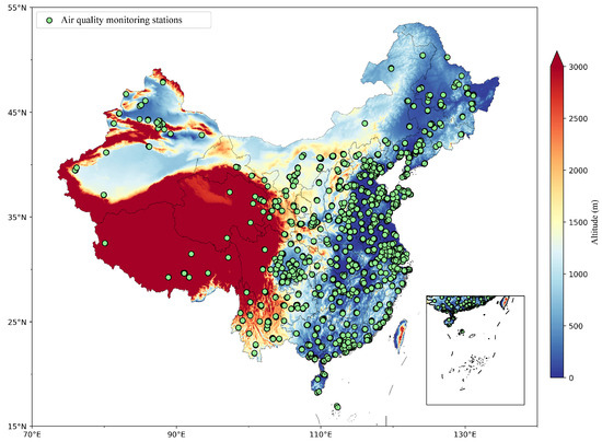
Figure 1.
Study area. The region covered in this study includes the entire territory of China. The green dots represent air quality monitoring stations.
Meteorological factors and geographic information influence the formation and accumulation of pollutants, making these variables essential for constructing particle estimation models. Meteorological factors were obtained from ERA5 data provided by the European Centre for Medium-Range Weather Forecasts (https://cds.climate.copernicus.eu/cdsapp#!/dataset/, accessed on 1 May 2023), which has a temporal resolution of hourly data and a spatial resolution of 0.25° × 0.25° [46]. This study incorporates factors, including boundary layer height (BLH, m), 2 m air temperature (TM, K), relative humidity (RH, %), wind speed (WS, m/s), wind direction (WD), surface solar radiation (SOR, W/m2), and surface pressure (SP, Pa), all of which are known to affect particle concentration [47,48,49].
This study uses the high and low vegetation indices (LH, LL) from ERA5 data to capture spatiotemporal variations in surface vegetation, with a spatial resolution of 0.25° × 0.25°. Elevation data (HEIGHT) were included in the model, sourced from the Gridded Global Topography dataset provided by the National Oceanic and Atmospheric Administration (NOAA) at a resolution of 1 km (https://www.ngdc.noaa.gov/mgg/topo, accessed on 1 May 2023). Considering regional land type differences, this research includes land cover type data (LUCC) obtained from satellite remote sensing of Terra and Aqua at a resolution of 0.05° × 0.05° (https://lpdaac.usgs.gov/products/mcd12c1v006/, accessed on 1 May 2023). Additionally, population density and total population data were included into the model, adjusted from the 2015 United Nations GPWv4 census-based dataset provided by NASA’s Socioeconomic Data and Applications Center (SEDAC) (http://sedac.ciesin.columbia.edu/data/collection/gpw-v4/documentation, accessed on 1 May 2023), which adjusts for relative spatial distribution across the country.
2.3. Data-Matching Method
The resolution of the meteorological data, elevation, land use types, and population density data was adjusted to 4 km using bilinear interpolation. To match the site data with grid data, a 0.04° × 0.04° grid covering China (70°E–140°E, 15°N–55°N) was established based on the spatial resolution of FY-4A. For station data, if a site fell within a specific grid, the observations from that site were used as the PM10 and PM2.5 values for that grid point. If a grid contained two or more sites, the average PM10 and PM2.5 values from those sites were assigned to that grid point. Finally, all data were matched with the 0.04° × 0.04° data grid of the FY-4A satellite.
2.4. Machine Learning Model
This study employed an ensemble learning method known as Extra Trees (ET) [50], which is composed of multiple decision trees. ET utilizes all samples for training and randomly selects features from those samples. The key characteristics of ET include the following:
(1) Random Features: In a sample set D where each sample has M attributes, m attributes are randomly selected, with m ≪ M.
(2) Splitting Randomness: When splitting each node in a decision tree, one attribute is randomly chosen as the basis for the split.
After selecting samples and features, decision trees are constructed using the best splitting attributes. This process is repeated to create multiple optimal decision trees within the ET model. The final output is obtained by averaging the results from all the decision trees. Additionally, the ET model provides feature importance scores, enhancing the interpretability of the results. ET models have been widely applied in various studies for data estimation purposes [51,52]. For a detailed description of the ET model structure, refer to the related literature [21]. Three other machine learning models were also used to validate the performance of the particle concentration estimation model: the random forest model (RF), the gradient boosting regression tree (GBDT), and the Bagging regression model.
2.4.1. TOAR Filling Method Model
To improve the coverage of the TOAR data, this study first processed the TOAR data from FY-4A and FY-4B by separately removing clouds. The resulting cloudless TOAR data were then matched with meteorological and geographical information. Using this matched dataset and the ET model, a TOAR data filling model under assumed clear-sky conditions was developed. This model allows the estimation of the radiation reaching the satellite instruments from the Earth’s surface under clear-sky conditions at any time. This approach increases the spatial coverage of the TOAR data from 36% (FY-4A) and 29% (FY-4B) to 100%. The expression of the TOAR ET estimation model is shown in Equation (1):
The variables in the ET model, denoted as , represent the position of the grid, time and various TOAR data . The independent variables include radiation products from the ERA5 dataset, such as clear-sky direct solar radiation at the surface, forecast albedo, mean surface direct short-wave radiation flux under clear-sky conditions, mean surface net short-wave radiation flux under clear-sky conditions, mean top downward short-wave radiation flux, mean top net short-wave radiation flux under clear-sky conditions, TOA incident solar radiation, and top net thermal radiation under clear-sky conditions. Additionally, meteorological factors such as boundary layer height (BLH), relative humidity (RH), 2 m air temperature (TM), and surface pressure (SP) are also included.
2.4.2. TOAR-Particulate Matter Estimation Model
This study developed ET models for estimating particulate matter concentrations using two types of TOAR datasets: cloud-removed TOAR data and TOAR data filled under assumed clear-sky conditions. Meteorological and geographical data used for each TOAR dataset were consistent, with matched station data serving as labels for the models. The formula for the TOAR-particulate matter ET estimation model is shown in Equation (2):
Here,represents the ET model, denotes the grid location, represents time, and indexes various TOAR datasets. The dependent variables are PM10 and PM2.5, and the independent variables include TOAR, boundary layer height (BLH), relative humidity (RH), 2 m air temperature (TM), and surface pressure (SP).
2.4.3. Model Validation Metrics
In this study, ten-fold cross-validation was employed to assess model performance [53]: all samples were randomly divided into ten subsets, with nine subsets used for training the ET model and the remaining subset used for training. This process was repeated ten times. The performance metrics used to describe the model include the coefficient of determination (R2), root-mean-square error (RMSE), and mean absolute error (MAE). The formula for each evaluation metric is as follows:
In the TOAR filling model, represents the error between model estimates and the mean of TOAR satellite observations . represents the total error between TOAR satellite observations and their mean. In the TOAR-particulate matter estimation model, represents the error between model estimates and the mean of particulate matter observations . at stations represents the total error between particulate matter station observations and their mean.
2.5. HYSPLIT Model
The HYSPLIT model, jointly developed over the past 20 years by the NOAA Air Resources Laboratory, is a specialized tool used for computing and analyzing the transport and dispersion trajectories of atmospheric pollutants [54]. HYSPLIT is widely used for the calculation and analysis atmospheric pollutant trajectories [55,56,57]. It can compute air mass trajectories and simulate complex dispersion and deposition processes. Backward trajectory analysis helps determine the origin of air masses (i.e., source tracing), while forward trajectory analysis projects their future paths, making it valuable for trajectory forecasting.
2.6. Meteorological Normalization Method
Meteorology and emissions significantly impact particulate matter concentrations. Meteorological normalization of particulate matter concentrations involves calculating the concentration for a specific time by averaging 1000 predictions from the ET model, while resampling meteorological variables from a specific period (December 2022 to March 2023). In this process, all meteorological variables are replaced with variables from any time within the specified period. As a result, particulate matter concentrations after meteorological normalization are interpreted as reflecting the environmental emission levels at that specific time [58,59].
2.7. SHAP Analysis Method
Due to the “black box” nature of most machine learning models, their results often lack reliable interpretability in terms of physical understanding [60]. However, with the development of feature attribution techniques, researchers now have tools to explore feature importance. One such method, based on game theory, is SHAP (Shapley Additive Explanations), which quantifies the global and local impacts of input features on model predictions, can provide the feature importance of each sample, and enables the detailed interpretation of a single sample [61]. But SHAP is computationally complex, and a list of high-impact values does not guarantee that it represents the best combination of inputs. Currently, it has been widely used in many fields [62,63,64], including in atmospheric science [65,66,67,68]. By employing the SHAP method, it is possible to enhance the physical interpretation of the contributors or driving factors of air pollution [69].
3. Model Performance
3.1. Performance of the TOAR Filling Method Using the ET Model
Due to the impact of cloud cover, obtaining fully covered TOAR data at all times was impractical. Therefore, we utilized cloud-free TOAR data, along with meteorological factors and geographic information, to build estimation models using ET. We then calculated fully covered TOAR data and replaced this with the cloudless TOAR data. The resulting TOAR data can be considered fully covered under assumed clear-sky conditions. Figure 2 illustrates the model’s performance in estimating TOAR under assumed clear-sky conditions. The results show that the R2 values for the estimated TOAR data from FY-4A and FY-4B satellites are above 0.85, with TOAR-3 exceeding 0.9. The RMSE for each TOAR channel data is generally around 0.02. Spatial validation of the TOAR data imputation model shows consistency with sample validation (Figure S1), indicating high temporal resolution at the hourly level. Next, we verified whether assumed clear-sky TOAR data could be applied to particulate matter estimation studies.
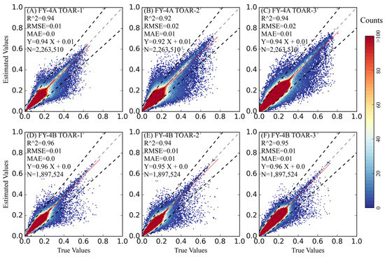
Figure 2.
Performance of the TOAR data estimation model. The dark dotted line represents the error line, the light dotted line represents the 1:1 line, and the solid red line represents the linear regression fitting line.
3.2. Performance Comparison of Original TOAR and Estimated TOAR in Constructing Particulate Matter Estimation ET Models
The presence of clouds in the Earth’s atmosphere often compromises satellite remote sensing of the Earth’s surface, making it challenging to obtain ground-based observational data [70,71]. Here, this study first examined the performance of PM10 and PM2.5 estimation models constructed under cloud removal conditions using TOAR data from FY-4A and FY-4B satellites. The models built with cloudless TOAR data from FY-4A and FY-4B present moderate performance, as illustrated in Figure S2, with R2 values of 0.76, 0.78, 0.8, and 0.81 and RMSE values of 13.86 μg/m3, 13.86 μg/m3, 6.66 μg/m3, and 6.74 μg/m3, respectively. Then, this study matched the estimated TOAR data under assumed clear-sky conditions, along with meteorological data and geographic information, to site observation data using the ET model. The performance of the model when estimating particulate matter concentrations using assumed clear-sky TOAR data is shown in Figure 3. Additionally, the performance comparison of the other three machine learning models (RF, GBDT, and Bagging) with the ET model is listed in Table S1. Considering the calculation cost and model performance, the ET model was selected to estimate the particulate matter concentration. The model exhibits significantly improved performance in estimating particulate matter (R2 improved by 0.02 to 0.06), especially for PM10 (FY-4A’s PM10 and PM2.5 models with R2 values of 0.82 and 0.82 and RMSE values of 31.95 μg/m3 and 13.29 μg/m3, respectively; FY-4B’s PM10 and PM2.5 models with R2 values of 0.83 and 0.83 and RMSE values of 31.43 μg/m3 and 13.03 μg/m3, respectively).
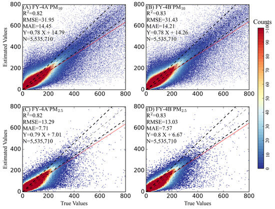
Figure 3.
Full coverage TOAR: particulate matter estimation model based on sample cross-validation results. The dark dotted line represents the error line, the light dotted line represents the 1:1 line, and the solid red line represents the linear regression fitting line.
Regarding spatial performance, the ET model demonstrates good spatial prediction capabilities. Based on site validation results (Figure 4), the PM10 and PM2.5 models for FY-4A indicate R2 values of 0.76 and 0.78, with RMSE values of 37.03 μg/m3 and 14.75 μg/m3, respectively. Similarly, for FY-4B, the PM10 and PM2.5 models exhibit R2 values of 0.78 and 0.79, with RMSE values of 36.16 μg/m3 and 14.4 μg/m3, respectively. Compared to sample-based validation, the precision changes minimally in spatial validation, indicating that the ET model can effectively estimate hourly PM10 and PM2.5 concentrations. Additionally, the estimation results suggest that FY-4A and FY-4B data perform similarly in estimating particulate matter products, although FY-4B illustrates slightly better estimation performance than FY-4A (especially in spatial validation). In order to facilitate the comparison of model performance of the two datasets, R2, RMSE, and MAE are shown in Table S2.
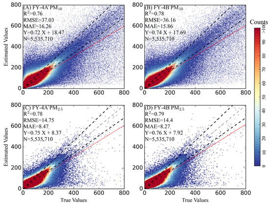
Figure 4.
Full coverage TOAR: particulate matter estimation model based on spatial validation results. The dark dotted line represents the error line, the light dotted line represents the 1:1 line, and the solid red line represents the linear regression fitting line.
3.3. Spatial Distribution of Particulate Matter Estimation Results
Particulate matter data estimated from 08:00 to 18:00 each day were averaged to create annual average particulate matter products, as shown in Figure 5. The 0.04° × 0.04° resolution PM10 and PM2.5 products estimated from FY-4A and FY-4B satellites exhibit spatial patterns that closely resemble those of corresponding site observation products. The average concentrations of PM10 and PM2.5 are approximately 59.1 ± 17.6 μg/m3 and 27.17 ± 6.1 μg/m3, respectively, with similar values estimated from both FY-4A and FY-4B.
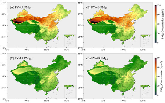
Figure 5.
The annual average distribution of the particulate matter estimation results.
The most severe PM10 pollution occurs in the Taklimakan Desert [72,73], where many areas experience high PM10 concentrations (>80 μg/m3). Elevated PM10 pollution levels are also observed in eastern Inner Mongolia, the North China Plain, and the Fenwei Plain, largely due to dense human activities as well as specific terrain and meteorological conditions [74,75]. In contrast, high annual average PM2.5 concentrations are found in the Fenwei Plain, North China Plain, and Sichuan Basin (especially in some point-like distributions in urban areas with high pollution levels) [76]. Overall, lower particulate matter concentrations are observed in the Qinghai–Tibet Plateau and the Pearl River Delta.
During the study period, more than 30% of China’s regions experienced high annual average particulate matter pollution levels that exceeded national air quality standards (PM2.5 > 35 μg/m3, PM10 > 75 μg/m3) [77,78]. Figure S3 displays the seasonal average spatial distribution of PM10 and PM2.5 based on estimated daily data from 08:00 to 18:00. The average PM10 concentrations are 32.1 ± 12.2 μg/m3, 43.9 ± 12.3 μg/m3, 66.4 ± 15.5 μg/m3, and 94.0 ± 38.4 μg/m3 in summer, autumn, winter, and spring, respectively. The average PM2.5 concentrations are 14.0 ± 3.4 μg/m3, 21.9 ± 5.7 μg/m3, 40.7 ± 12.9 μg/m3, and 32.0 ± 7.5 μg/m3 in the same respective seasons. The spatial distribution of PM10 and PM2.5 demonstrates significant seasonal variations, with higher values observed in spring and winter (corresponding to periods of dust and haze in China) [79], while lower pollution levels are observed in summer and autumn.
4. Interpretable Machine Learning Analysis of Particulate Matter Pollution Events
4.1. Influence of Meteorological Factors on Dust Transport Processes
From 19 to 23 March 2023, China experienced a severe dust storm event [80]. This event was the most intense and widespread dust storm since 2023, affecting 20 provinces and covering an area exceeding 4.85 million square kilometers, achieving the level of severe-dust-storm intensity. As shown in Figure 6, starting on the 21st, the dust gradually spread into Inner Mongolia, the North China Plain, the Guanzhong Plain, and the Shandong Peninsula and continued spreading until the storm began to weaken on the 24th. During the dust storm, PM10 concentrations surged to over 240 μg/m3, whereas PM2.5 concentrations remained relatively stable. Although dust particles are well-known as the primary factor in dust storms, the impact of various meteorological variables in the development and progression of such events remains a crucial area of investigation [81].
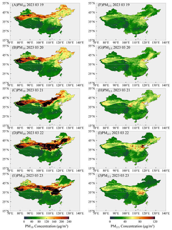
Figure 6.
Spatial distribution of PM10 and PM2.5 concentrations during the development of the dust storm event. (Left) Distribution of PM10 concentrations. (Right) Distribution of PM2.5 concentrations.
First, the meteorologically normalized values of PM10 and PM2.5 for March 2023 were calculated. The difference between the PM10 and PM2.5 concentrations during the dust storm period and these normalized values yielded the increments (ΔPM10 and ΔPM2.5). Subsequently, five locations affected by the dust storm were randomly selected (see Figure S5), and four backward trajectories were modeled for each location using the HYSPLIT model. The positions (latitude and longitude), heights, pressures, temperatures (TM), surface pressures (SP), wind speeds (WS), relative humidities (RH), boundary layer heights (BLH), surface solar radiation (SOR), land use and land cover (LUCC), altitude (HEIGHT), and population density (RK) along each trajectory were compared with ΔPM10 and ΔPM2.5 (changes in PM10 and PM2.5).
The modeling results, shown in Figure 7, yielded R2 values of 0.69 and 0.65, indicating that the model effectively describes the relationship between meteorological elements along trajectory paths and variations in ΔPM10 and ΔPM2.5 during the dust storm. To further understand the relationship between meteorological elements along trajectory paths and variations in ΔPM10 and ΔPM2.5, feature importance was assessed from the ET model’s built-in interpreter. The results (Table 2) highlight two key findings: First, the dust storm was driven from northwest to southeast by the Mongolian cyclone, marking latitude and longitude, which represent crucial trajectory positions. Second, significant fluctuations in surface pressure and wind speed accompanied the movement of the Mongolian cyclone, exerting considerable influence on dust transport. Among the remaining variables, land use and land cover had minimal impact, suggesting that the dust storm primarily involved upper-level dust transport, with surface characteristics playing a lesser role.
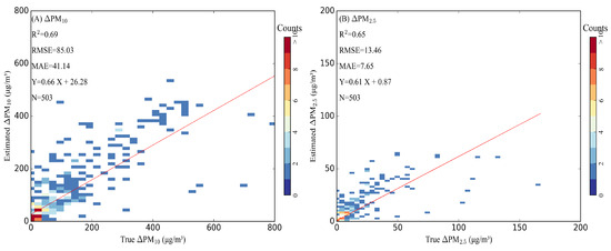
Figure 7.
Interpretation of the dust transport model for ΔPM10 and ΔPM2.5.The solid red line represents the linear regression fitting line.

Table 2.
Feature importance of the dust transport model.
However, it is important to note that feature importance reflects only the relative importance of each input variable in model construction rather than the direct physical contribution of influencing factors to ΔPM10 and ΔPM2.5. While feature importance analysis provides initial insights into which features significantly affect model predictions, an additional analysis is required to determine the specific impact of each feature on ΔPM10 and ΔPM2.5.
To understand the model’s decision-making mechanism, a SHAP analysis of the ΔPM10 model was conducted, which revealed the contributions of various variables to the increase in PM10 concentrations during dust transport. According to the data shown in Figure 8, higher latitude values are associated with lower particulate matter concentrations (red areas for latitude and negative SHAP values), while lower latitude values are associated with higher particulate matter concentrations. Higher temperatures correspond to higher particulate matter concentrations (red areas for temperature and positive SHAP values), whereas lower temperatures are associated with SHAP values in the ranging from −50 to 0. Additionally, relative humidity also ranks high in influence, aligning with findings from previous studies [82]. Simultaneously, higher atmospheric pressure at the altitude of the air mass correlates with more pronounced increases in PM10 concentrations, indicating the significant influence of high-altitude dust descent on surface PM10 levels [83]. Atmospheric pressure and wind speed play crucial roles under the influence of the Mongolian cyclone: higher atmospheric pressure typically leads to increased PM10 concentrations, while wind speed affects dust storms in two ways: by intensifying their severity during onset and potentially dispersing dust particles, thereby reducing PM10 levels [80,84]. Furthermore, surface solar radiation intensity (SOR) significantly impacts PM10 concentrations by increasing the reflection of solar radiation from the ground, which closely correlates with PM10 concentration increases [85]. In contrast, PM2.5 is more influenced by relative humidity and temperature.
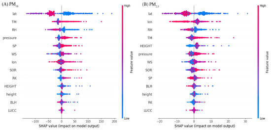
Figure 8.
SHAP importance scores of variables impacting ΔPM10 and ΔPM2.5 during dust storm processes. The variables shown in the figure include the following: lat: latitude, lon: longitude, height: air mass height, pressures: the air pressure at the height of the air mass, TM: temperatures, SP: surface pressures, WS: wind speeds, RH: relative humidities, BLH: boundary layer heights, SOR: surface solar radiation, LUCC: land use and land cover, HEIGHT: altitude, and RK: population density.
4.2. Influence of Meteorological Factors in Haze Weather Event
During the haze weather event in northern China from 7 to 10 December 2022, regions such as the Fenwei Plain, Henan, Shandong, southern Hebei, northern Anhui, and northwest Jiangsu experienced a significant increase in PM2.5 concentrations. A comparison between normalized meteorological particle concentrations and actual particle concentrations, as shown in Figure 9 and Figure S6, revealed significant increases in PM2.5 levels during this period. A further SHAP analysis provided insights into the effects of various meteorological variables on particle concentrations during these haze events.
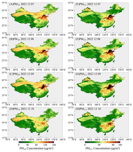
Figure 9.
Distribution of PM2.5 and PM10 concentrations during the development of the haze event. Left: Distribution of PM10 concentrations. Right: Distribution of PM2.5 concentrations.
Similarly, by subtracting normalized meteorological particle concentrations from those observed during haze events, ΔPM10 and ΔPM2.5 were derived. The SHAP values calculated for each variable from December 7th to 10th further elucidate these influences. As shown in Figure 10, haze processes have a greater impact on PM2.5 than on PM10, as indicated by the total SHAP values for each. On 7 December, during the pollution formation period, the primary influencing factors were temperature (TM), pressure (SP), and boundary layer height (BLH). Here, the higher SHAP values for temperature and pressure suggest that lower temperatures and higher pressures contribute to pollutant accumulation, while boundary layer height affects pollutant dispersion and dilution significantly. During the pollution outbreak period from 8 to 9 December, pressure (SP), temperature (TM), and relative humidity (RH) emerged as the main influencing factors. The persistent high SHAP values for pressure and temperature indicate their continued role in pollutant concentration. Additionally, the influence of relative humidity indicates that increased humidity may cause hygroscopic growth of particles, thereby increasing PM2.5 concentrations. On 10 December, during the pollution dissipation period, while pressure (SP) and relative humidity (RH) remaining as major influencing factors, wind speed (WS) showed a significant increase in influence. This suggests that wind speed plays a crucial role in pollutant dispersion during the pollution dissipation period. Additionally, solar radiation (SOR), which reflects the reduction in radiation received at the ground due to particles, and altitude (HEIGHT), which affects pollutant dispersion, also contributed to the model’s outcomes. Overall, meteorological factors exhibit complex and multifaceted effects on particulate matter concentrations. Although the primary influencing factors vary over time, pressure, temperature, and boundary layer height consistently emerge as major factors.
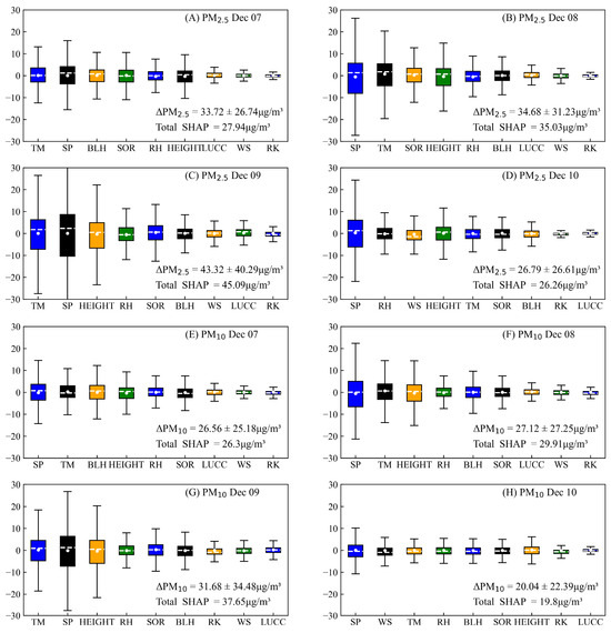
Figure 10.
SHAP importance scores of various variables affecting ΔPM10 and ΔPM2.5 during haze weather.
5. Conclusions
Using satellite data to obtain ground-level pollutant distribution information is a key focus of current research. The FY-4A and FY-4B geostationary meteorological satellites represent China’s new generation of geostationary observation satellite systems. Previous studies have shown that FY-4A’s TOAR data can accurately retrieve particulate matter concentrations across China. However, earlier estimations of near-surface particulate matter concentrations have faced challenges due to cloud interference, resulting in low data coverage and an inability to continuously monitor pollutant variations. In this study, we employed the TOAR data filling method to generate fully covered, high-spatiotemporal-resolution PM10 and PM2.5 data products. This approach increased data coverage from 36% (FY-4A) and 29% (FY-4B) to 100%. Our findings indicate that the model performance in estimating particulate matter concentrations under assumed clear-sky conditions using TOAR data outperformed that of models using cloud-removed TOAR data, achieving R-squared values above 0.8 when comparing the TOAR data under clear-sky conditions to the original TOAR data. We also compared the performance of FY-4A and FY-4B TOAR data in estimating particulate matter estimation. Both satellites’ data can effectively estimate particulate matter concentrations, exhibiting similar performance in their respective ET models. Combining station observation data with TOAR data assumed under clear-sky conditions significantly improved the model’s ability to estimate particulate matter concentrations, particularly raising the R-squared value for PM10 to 0.83. Spatial verification results also indicate that the estimation model can effectively reflect spatiotemporal variations in particulate matter concentrations. Annual average concentration products for PM10 and PM2.5 indicate that the Taklimakan Desert, eastern Inner Mongolia, the North China Plain, and the Fenwei Plain are high-pollution areas for PM10, while the Fenwei Plain, North China Plain, and Sichuan Basin are high-pollution areas for PM2.5. This study provides a scientific basis for monitoring and controlling particulate matter pollution, emphasizing the crucial role of meteorological factors in particulate matter concentration changes. In the future, more accurate particulate matter concentration information for China can be obtained based on dual-satellite observations.
The estimated hourly particulate matter concentration provides valuable insights into pollutant development and specific distribution scenarios. Through studies of strong spring sandstorms in northern China in 2023 and haze weather processes in December 2022, meteorological factors’ significant role in particulate matter concentration changes is revealed. During sandstorm events, PM10 concentrations significantly rise above 240 μg/m3, severely affecting air quality, transportation, and public health. The HYSPLIT model and SHAP analysis indicate that the characteristics of air mass location, air mass height, air pressure, and wind speed have great influence on PM10 concentration changes. High pressure and low temperatures lead to dust particle accumulation, while wind speed may exacerbate or alleviate the impact of sandstorms. In hazy weather, pressure, temperature, and boundary layer height are major influencing factors. Low temperatures and high pressure lead to pollutant accumulation, while a low boundary layer height restricts pollutant dispersion. Additionally, increased relative humidity causes particle hygroscopic growth. Wind speed also significantly affects particle concentration during pollution dissipation periods. SHAP analysis reveals significant spatiotemporal differences in meteorological factors’ impact on particle concentration changes, thereby providing a scientific basis for pollution control measures.
Overall, the TOAR-particulate matter model constructed using the TOAR filling method excels in temporal resolution, spatial resolution, and model accuracy compared to previous related studies. This research demonstrates that China’s high spatiotemporal resolution fully covered particulate matter dataset will play a role in future atmospheric pollution studies at medium or small scales.
Supplementary Materials
The following supporting information can be downloaded at https://www.mdpi.com/article/10.3390/rs16183363/s1. Tables S1 and S2; Figures S1–S6.
Author Contributions
Z.S.: software, methodology, data curation, and writing—original draft. B.C.: conceptualization, methodology, and writing—review and editing. L.Z. and Q.Y.: writing—original draft. Y.R. and R.C.: software. All authors have read and agreed to the published version of the manuscript.
Funding
This work was supported by the Fundamental Research Funds for the Central Universities (grant number lzujbky-2023-ey10), the Gansu Provincial Science and Technology Plan (grant number 23JRRA1038), and the National Natural Science Foundation of China (grant number 41775021).
Data Availability Statement
The PM2.5 and PM10 data were obtained from https://www.aqistudy.cn/historydata/ (accessed on 1 May 2023). The FY-4A and FY-4B data were provided by the National Satellite Meteorological Center of China; these can be downloaded from http://satellite.nsmc.org.cn/PortalSite/Data/Satellite.aspx (accessed on 1 May 2023). The ERA-5 data are available from https://cds.climate.copernicus.eu/cdsapp#!/dataset/reanalysis-era5-land?tab=overview (accessed on 1 May 2023).
Acknowledgments
The authors would like to thank the China National Environmental Monitoring Center, National Satellite Meteorological Center of China, European Centre for Medium-Range Weather Forecasts, and NASA for their datasets.
Conflicts of Interest
The authors declare no conflicts of interest.
References
- WHO. Particulate matter (PM2.5 and PM10), ozone, nitrogen dioxide, sulfur dioxide and carbon monoxide. In WHO Global Air Quality Guidelines; World Health Organization: Geneva, Switzerland, 2021. [Google Scholar]
- Zhang, Q.; Zheng, Y.; Tong, D.; Shao, M.; Wang, S.; Zhang, Y.; Xu, X.; Wang, J.; He, H.; Liu, W.; et al. Drivers of improved PM2.5 air quality in China from 2013 to 2017. Proc. Natl. Acad. Sci. USA 2019, 116, 24463–24469. [Google Scholar] [CrossRef] [PubMed]
- Yang, Y.; Zeng, L.; Wang, H.; Wang, P.; Liao, H. Dust pollution in China affected by different spatial and temporal types of El Niño. Atmos. Chem. Phys. 2022, 22, 14489–14502. [Google Scholar] [CrossRef]
- Yang, Y.; Liao, H.; Lou, S. Increase in winter haze over eastern China in recent decades: Roles of variations in meteorological parameters and anthropogenic emissions. J. Geophys. Res. Atmos. 2016, 121, 13050–13065. [Google Scholar] [CrossRef]
- Crouse, D.L.; Peters, P.A.; Donkelaar, A.v.; Goldberg, M.S.; Villeneuve, P.J.; Brion, O.; Khan, S.; Atari, D.O.; Jerrett, M.; Pope, C.A.; et al. Risk of Nonaccidental and Cardiovascular Mortality in Relation to Long-term Exposure to Low Concentrations of Fine Particulate Matter: A Canadian National-Level Cohort Study. Environ. Health Perspect. 2012, 120, 708–714. [Google Scholar] [CrossRef] [PubMed]
- Xing, Y.-F.; Xu, Y.-H.; Shi, M.-H.; Lian, Y.-X. The impact of PM2.5 on the human respiratory system. J. Thorac. Dis. 2016, 8, E69–E74. [Google Scholar]
- Zhang, Q.; Jiang, X.; Tong, D.; Davis, S.J.; Zhao, H.; Geng, G.; Feng, T.; Zheng, B.; Lu, Z.; Streets, D.G.; et al. Transboundary health impacts of transported global air pollution and international trade. Nature 2017, 543, 705–709. [Google Scholar] [CrossRef] [PubMed]
- Pope III, C.A.; Burnett, R.T.; Thun, M.J.; Calle, E.E.; Krewski, D.; Ito, K.; Thurston, G.D. Lung Cancer, Cardiopulmonary Mortality, and Long-term Exposure to Fine Particulate Air Pollution. JAMA 2002, 287, 1132–1141. [Google Scholar] [CrossRef] [PubMed]
- Pu, W.; Cui, J.; Wu, D.; Shi, T.; Chen, Y.; Xing, Y.; Zhou, Y.; Wang, X. Unprecedented snow darkening and melting in New Zealand due to 2019–2020 Australian wildfires. Fundam. Res. 2021, 1, 224–231. [Google Scholar] [CrossRef]
- Yang, Y.; Zhou, Y.; Li, K.; Wang, H.; Ren, L.; Zeng, L.; Li, H.; Wang, P.; Li, B.; Liao, H. Atmospheric Circulation Patterns Conducive to Severe Haze in Eastern China Have Shifted Under Climate Change. Geophys. Res. Lett. 2021, 48, e2021GL095011. [Google Scholar] [CrossRef]
- Yang, Y.; Ren, L.; Li, H.; Wang, H.; Wang, P.; Chen, L.; Yue, X.; Liao, H. Fast Climate Responses to Aerosol Emission Reductions During the COVID-19 Pandemic. Geophys. Res. Lett. 2020, 47, e2020GL089788. [Google Scholar] [CrossRef]
- Wei, J.; Huang, W.; Li, Z.; Xue, W.; Peng, Y.; Sun, L.; Cribb, M. Estimating 1-km-resolution PM2.5 concentrations across China using the space-time random forest approach. Remote Sens. Environ. 2019, 231, 111221. [Google Scholar] [CrossRef]
- Li, Y.; Wang, W.; Han, Y.; Liu, W.; Wang, R.; Zhang, R.; Zhao, Z.; Sheng, L.; Zhou, Y. Impact of COVID-19 emission reduction on dust aerosols and marine chlorophyll-a concentration. Sci. Total Environ. 2024, 918, 170493. [Google Scholar] [CrossRef] [PubMed]
- Guo, J.; Xia, F.; Zhang, Y.; Liu, H.; Li, J.; Lou, M.; He, J.; Yan, Y.; Wang, F.; Min, M.; et al. Impact of diurnal variability and meteorological factors on the PM2.5—AOD relationship: Implications for PM2.5 remote sensing. Environ. Pollut. 2017, 221, 94–104. [Google Scholar] [CrossRef] [PubMed]
- Chen, S.; Tong, B.; Russell, L.M.; Wei, J.; Guo, J.; Mao, F.; Liu, D.; Huang, Z.; Xie, Y.; Qi, B.; et al. Lidar-based daytime boundary layer height variation and impact on the regional satellite-based PM2.5 estimate. Remote Sens. Environ. 2022, 281, 113224. [Google Scholar] [CrossRef]
- Ma, X.; Wang, J.; Yu, F.; Jia, H.; Hu, Y. Can MODIS AOD be employed to derive PM2.5 in Beijing-Tianjin-Hebei over China? Atmos. Res. 2016, 181, 250–256. [Google Scholar] [CrossRef]
- Yao, F.; Si, M.; Li, W.; Wu, J. A multidimensional comparison between MODIS and VIIRS AOD in estimating ground-level PM2.5 concentrations over a heavily polluted region in China. Sci. Total Environ. 2018, 618, 819–828. [Google Scholar] [CrossRef]
- You, W.; Zang, Z.; Pan, X.; Zhang, L.; Chen, D. Estimating PM2.5 in Xi’an, China using aerosol optical depth: A comparison between the MODIS and MISR retrieval models. Sci. Total Environ. 2015, 505, 1156–1165. [Google Scholar] [CrossRef]
- Ye, H.; Pan, X.; You, W.; Zhu, X.; Zang, Z.; Wang, D.; Zhang, X.; Hu, Y.; Jin, S. Impact of CALIPSO profile data assimilation on 3-D aerosol improvement in a size-resolved aerosol model. Atmos. Res. 2021, 264, 105877. [Google Scholar] [CrossRef]
- Zhang, Y.; Li, Z.; Bai, K.; Wei, Y.; Xie, Y.; Zhang, Y.; Ou, Y.; Cohen, J.; Zhang, Y.; Peng, Z.; et al. Satellite remote sensing of atmospheric particulate matter mass concentration: Advances, challenges, and perspectives. Fundam. Res. 2021, 1, 240–258. [Google Scholar] [CrossRef]
- Chen, B.; Song, Z.; Pan, F.; Huang, Y. Obtaining vertical distribution of PM2.5 from CALIOP data and machine learning algorithms. Sci. Total Environ. 2022, 805, 150338. [Google Scholar] [CrossRef]
- Vu, B.N.; Bi, J.; Wang, W.; Huff, A.; Kondragunta, S.; Liu, Y. Application of geostationary satellite and high-resolution meteorology data in estimating hourly PM2.5 levels during the Camp Fire episode in California. Remote Sens. Environ. 2022, 271, 112890. [Google Scholar] [CrossRef] [PubMed]
- Pang, J.; Liu, Z.; Wang, X.; Bresch, J.; Ban, J.; Chen, D.; Kim, J. Assimilating AOD retrievals from GOCI and VIIRS to forecast surface PM2.5 episodes over Eastern China. Atmos. Environ. 2018, 179, 288–304. [Google Scholar] [CrossRef]
- Song, Z.; Chen, B.; Huang, J. Combining Himawari-8 AOD and deep forest model to obtain city-level distribution of PM2.5 in China. Environ. Pollut. 2022, 297, 118826. [Google Scholar] [CrossRef]
- Chen, B.; Song, Z.; Shi, B.; Li, M. An interpretable deep forest model for estimating hourly PM10 concentration in China using Himawari-8 data. Atmos. Environ. 2022, 268, 118827. [Google Scholar] [CrossRef]
- Tang, B.; Stanier, C.O.; Carmichael, G.R.; Gao, M. Ozone, nitrogen dioxide, and PM2.5 estimation from observation-model machine learning fusion over S. Korea: Influence of observation density, chemical transport model resolution, and geostationary remotely sensed AOD. Atmos. Environ. 2024, 331, 120603. [Google Scholar] [CrossRef]
- Thongsame, W.; Henze, D.K.; Kumar, R.; Barth, M.; Pfister, G. Evaluation of WRF-Chem PM2.5 simulations in Thailand with different anthropogenic and biomass-burning emissions. Atmos. Environ. X 2024, 23, 100282. [Google Scholar] [CrossRef]
- Yang, C.; Guan, L.; Sun, X. Comparison of FY-4A/AGRI SST with Himawari-8/AHI and In Situ SST. Remote Sens. 2023, 15, 4139. [Google Scholar] [CrossRef]
- Wang, W.; Mao, F.; Pan, Z.; Gong, W.; Yoshida, M.; Zou, B.; Ma, H. Evaluating Aerosol Optical Depth From Himawari-8 With Sun Photometer Network. J. Geophys. Res. Atmos. 2019, 124, 5516–5538. [Google Scholar] [CrossRef]
- Yin, J.; Mao, F.; Zang, L.; Chen, J.; Lu, X.; Hong, J. Retrieving PM2.5 with high spatio-temporal coverage by TOA reflectance of Himawari-8. Atmos. Pollut. Res. 2021, 12, 14–20. [Google Scholar] [CrossRef]
- Liu, J.; Weng, F.; Li, Z. Satellite-based PM2.5 estimation directly from reflectance at the top of the atmosphere using a machine learning algorithm. Atmos. Environ. 2019, 208, 113–122. [Google Scholar] [CrossRef]
- Wang, B.; Yuan, Q.; Yang, Q.; Zhu, L.; Li, T.; Zhang, L. Estimate hourly PM2.5 concentrations from Himawari-8 TOA reflectance directly using geo-intelligent long short-term memory network. Environ. Pollut. 2021, 271, 116327. [Google Scholar] [CrossRef] [PubMed]
- Chen, B.; Song, Z.; Huang, J.; Zhang, P.; Hu, X.; Zhang, X.; Guan, X.; Ge, J.; Zhou, X. Estimation of Atmospheric PM10 Concentration in China Using an Interpretable Deep Learning Model and Top-of-the-Atmosphere Reflectance Data From China’s New Generation Geostationary Meteorological Satellite, FY-4A. J. Geophys. Res. Atmos. 2022, 127, e2021JD036393. [Google Scholar] [CrossRef]
- Song, Z.; Chen, B.; Zhang, P.; Guan, X.; Wang, X.; Ge, J.; Hu, X.; Zhang, X.; Wang, Y. High temporal and spatial resolution PM2.5 dataset acquisition and pollution assessment based on FY-4A TOAR data and deep forest model in China. Atmos. Res. 2022, 274, 106199. [Google Scholar] [CrossRef]
- Hu, Y.; Zeng, C.; Li, T.; Shen, H. Performance comparison of Fengyun-4A and Himawari-8 in PM2.5 estimation in China. Atmos. Environ. 2022, 271, 118898. [Google Scholar] [CrossRef]
- Wang, S.; Lu, F.; Feng, Y. An Investigation of the Fengyun-4A/B GIIRS Performance on Temperature and Humidity Retrievals. Atmosphere 2022, 13, 1830. [Google Scholar] [CrossRef]
- Handschuh, J.; Erbertseder, T.; Baier, F. On the added value of satellite AOD for the investigation of ground-level PM2.5 variability. Atmos. Environ. 2024, 331, 120601. [Google Scholar] [CrossRef]
- Bagheri, H. A machine learning-based framework for high resolution mapping of PM2.5 in Tehran, Iran, using MAIAC AOD data. Adv. Space Res. 2022, 69, 3333–3349. [Google Scholar] [CrossRef]
- Pu, Q.; Yoo, E.-H. A gap-filling hybrid approach for hourly PM2.5 prediction at high spatial resolution from multi-sourced AOD data. Environ. Pollut. 2022, 315, 120419. [Google Scholar] [CrossRef]
- Yang, J.; Zhang, Z.; Wei, C.; Lu, F.; Guo, Q. Introducing the New Generation of Chinese Geostationary Weather Satellites, Fengyun-4. Bull. Am. Meteorol. Soc. 2017, 98, 1637–1658. [Google Scholar] [CrossRef]
- Zhang, Y.; Li, Z.; Li, J. A Preliminary Layer Perceptible Water Vapor Retrieval Algorithm for Fengyun-4 Advanced Geosynchronous Radiation Imager. In Proceedings of the IGARSS 2019—2019 IEEE International Geoscience and Remote Sensing Symposium, Yokohama, Japan, 28 July–2 August 2019; pp. 7564–7566. [Google Scholar]
- Cheng, Y.; Dai, T.; Goto, D.; Chen, L.; Si, Y.; Murakami, H.; Yoshida, M.; Zhang, P.; Cao, J.; Nakajima, T.; et al. Improved hourly estimate of aerosol optical thickness over Asian land by fusing geostationary satellites Fengyun-4B and Himawari-9. Sci. Total Environ. 2024, 923, 171541. [Google Scholar] [CrossRef]
- Gao, Y.; Wang, X.; Mao, D. Performance of FY-4B GIIRS temperature products under cloudy skies and their enhancement of surface precipitation type forecasting. Atmos. Res. 2024, 302, 107305. [Google Scholar] [CrossRef]
- Kikuchi, M.; Murakami, H.; Suzuki, K.; Nagao, T.M.; Higurashi, A. Improved Hourly Estimates of Aerosol Optical Thickness Using Spatiotemporal Variability Derived From Himawari-8 Geostationary Satellite. IEEE Trans. Geosci. Remote Sens. 2018, 56, 3442–3455. [Google Scholar] [CrossRef]
- Min, M.; Wu, C.; Li, C.; Liu, H.; Xu, N.; Wu, X.; Chen, L.; Wang, F.; Sun, F.; Qin, D.; et al. Developing the science product algorithm testbed for Chinese next-generation geostationary meteorological satellites: Fengyun-4 series. J. Meteorol. Res. 2017, 31, 708–719. [Google Scholar] [CrossRef]
- Hersbach, H.; Bell, B.; Berrisford, P.; Hirahara, S.; Horányi, A.; Muñoz-Sabater, J.; Nicolas, J.; Peubey, C.; Radu, R.; Schepers, D.; et al. The ERA5 global reanalysis. Q. J. R. Meteorol. Soc. 2020, 146, 1999–2049. [Google Scholar] [CrossRef]
- Miao, Y.; Che, H.; Zhang, X.; Liu, S. Relationship between summertime concurring PM2.5 and O3 pollution and boundary layer height differs between Beijing and Shanghai, China. Environ. Pollut. 2021, 268, 115775. [Google Scholar] [CrossRef]
- Tsao, T.-M.; Hwang, J.-S.; Chen, C.-Y.; Lin, S.-T.; Tsai, M.-J.; Su, T.-C. Urban climate and cardiovascular health: Focused on seasonal variation of urban temperature, relative humidity, and PM2.5 air pollution. Ecotoxicol. Environ. Saf. 2023, 263, 115358. [Google Scholar] [CrossRef]
- Jeong, Y.-C.; Yeh, S.-W.; Jeong, J.I.; Park, R.J.; Wang, Y. Existence of typical winter atmospheric circulation patterns leading to high PM2.5 concentration days in East Asia. Environ. Pollut. 2024, 348, 123829. [Google Scholar] [CrossRef]
- Geurts, P.; Ernst, D.; Wehenkel, L. Extremely randomized trees. Mach. Learn. 2006, 63, 3–42. [Google Scholar] [CrossRef]
- Zhang, Q.; Shi, R.; Singh, V.P.; Xu, C.-Y.; Yu, H.; Fan, K.; Wu, Z. Droughts across China: Drought factors, prediction and impacts. Sci. Total Environ. 2022, 803, 150018. [Google Scholar] [CrossRef]
- Ahmad, M.W.; Reynolds, J.; Rezgui, Y. Predictive modelling for solar thermal energy systems: A comparison of support vector regression, random forest, extra trees and regression trees. J. Clean. Prod. 2018, 203, 810–821. [Google Scholar] [CrossRef]
- Chen, B.; Chen, R.; Zhao, L.; Ren, Y.; Zhang, L.; Zhao, Y.; Lian, X.; Yan, W.; Gao, S. High-resolution short-term prediction of the COVID-19 epidemic based on spatial-temporal model modified by historical meteorological data. Fundam. Res. 2024, 4, 527–539. [Google Scholar] [CrossRef] [PubMed]
- Draxler, R.R.; Hess, G. An overview of the HYSPLIT_4 modelling system for trajectories. Aust. Meteorol. Mag. 1998, 47, 295–308. [Google Scholar]
- Gammoudi, N.; Kovács, J.; Gresina, F.; Varga, G. Combined use of HYSPLIT model and MODIS aerosols optical depth to study the spatiotemporal circulation patterns of Saharan dust events over Central Europe. Aeolian Res. 2024, 67–69, 100899. [Google Scholar] [CrossRef]
- Su, L.; Yuan, Z.; Fung, J.C.H.; Lau, A.K.H. A comparison of HYSPLIT backward trajectories generated from two GDAS datasets. Sci. Total Environ. 2015, 506–507, 527–537. [Google Scholar] [CrossRef] [PubMed]
- Iraji, F.; Memarian, M.H.; Joghataei, M.; Ghafarian Malamiri, H.R. Determining the source of dust storms with use of coupling WRF and HYSPLIT models: A case study of Yazd province in central desert of Iran. Dyn. Atmos. Ocean. 2021, 93, 101197. [Google Scholar] [CrossRef]
- Song, C.; Liu, B.; Cheng, K.; Cole, M.A.; Dai, Q.; Elliott, R.J.R.; Shi, Z. Attribution of Air Quality Benefits to Clean Winter Heating Policies in China: Combining Machine Learning with Causal Inference. Environ. Sci. Technol. 2023, 57, 17707–17717. [Google Scholar] [CrossRef]
- Grange, S.K.; Carslaw, D.C. Using meteorological normalisation to detect interventions in air quality time series. Sci. Total Environ. 2019, 653, 578–588. [Google Scholar] [CrossRef]
- Grange, S.K.; Carslaw, D.C.; Lewis, A.C.; Boleti, E.; Hueglin, C. Random forest meteorological normalisation models for Swiss PM10 trend analysis. Atmos. Chem. Phys. 2018, 18, 6223–6239. [Google Scholar] [CrossRef]
- Lundberg, S.M.; Lee, S.-I. A Unified Approach to Interpreting Model Predictions. In Proceedings of the Neural Information Processing Systems; Curran Associates Inc.: Red Hook, NY, USA, 2017; pp. 4768–4777. [Google Scholar]
- Yang, C.; Guan, X.; Xu, Q.; Xing, W.; Chen, X.; Chen, J.; Jia, P. How can SHAP (SHapley Additive exPlanations) interpretations improve deep learning based urban cellular automata model? Comput. Environ. Urban Syst. 2024, 111, 102133. [Google Scholar] [CrossRef]
- Antonini, A.S.; Tanzola, J.; Asiain, L.; Ferracutti, G.R.; Castro, S.M.; Bjerg, E.A.; Ganuza, M.L. Machine Learning model interpretability using SHAP values: Application to Igneous Rock Classification task. Appl. Comput. Geosci. 2024, 23, 100178. [Google Scholar] [CrossRef]
- Aldrees, A.; Khan, M.; Taha, A.T.B.; Ali, M. Evaluation of water quality indexes with novel machine learning and SHapley Additive ExPlanation (SHAP) approaches. J. Water Process Eng. 2024, 58, 104789. [Google Scholar] [CrossRef]
- Tao, C.; Zhu, T.; Fu, D.; Yan, B.; Li, H. Toward better atmospheric polycyclic aromatic hydrocarbons pollution control in the Northern Hemisphere: Process analysis based on interpretable deep learning models. J. Clean. Prod. 2024, 457, 142442. [Google Scholar] [CrossRef]
- Chen, W.; Xu, X.; Liu, W. Combined PMF modelling and machine learning to identify sources and meteorological influencers of volatile organic compound pollution in an industrial city in eastern China. Atmos. Environ. 2024, 334, 120714. [Google Scholar] [CrossRef]
- Yin, H.; Sun, Y.; You, Y.; Notholt, J.; Palm, M.; Wang, W.; Shan, C.; Liu, C. Using machine learning approach to reproduce the measured feature and understand the model-to-measurement discrepancy of atmospheric formaldehyde. Sci. Total Environ. 2022, 851, 158271. [Google Scholar] [CrossRef] [PubMed]
- Peng, Z.; Zhang, B.; Wang, D.; Niu, X.; Sun, J.; Xu, H.; Cao, J.; Shen, Z. Application of machine learning in atmospheric pollution research: A state-of-art review. Sci. Total Environ. 2024, 910, 168588. [Google Scholar] [CrossRef]
- Liu, X.; Wang, L.; Huang, J.; Wang, Y.; Li, C.; Ding, L.; Lian, X.; Shi, J. Revealing the Covariation of Atmospheric O2 and Pollutants in an Industrial Metropolis by Explainable Machine Learning. Environ. Sci. Technol. Lett. 2023, 10, 851–858. [Google Scholar] [CrossRef]
- Yang, P.; Meyer, K. Satellites and Satellite Remote Sensing|Remote Sensing: Cloud Properties. In Reference Module in Earth Systems and Environmental Sciences; Elsevier: Amsterdam, The Netherlands, 2024. [Google Scholar]
- Chi, Y.; Zhao, C.; Yang, Y.; Zhao, X.; Yang, J. Global characteristics of cloud macro-physical properties from active satellite remote sensing. Atmos. Res. 2024, 302, 107316. [Google Scholar] [CrossRef]
- Wang, J.; Gui, H.; An, L.; Hua, C.; Zhang, T.; Zhang, B. Modeling for the source apportionments of PM10 during sand and dust storms over East Asia in 2020. Atmos. Environ. 2021, 267, 118768. [Google Scholar] [CrossRef]
- Guan, Q.; Luo, H.; Pan, N.; Zhao, R.; Yang, L.; Yang, Y.; Tian, J. Contribution of dust in northern China to PM10 concentrations over the Hexi corridor. Sci. Total Environ. 2019, 660, 947–958. [Google Scholar] [CrossRef]
- Wang, Y.; Yuan, Q.; Li, T.; Tan, S.; Zhang, L. Full-coverage spatiotemporal mapping of ambient PM2.5 and PM10 over China from Sentinel-5P and assimilated datasets: Considering the precursors and chemical compositions. Sci. Total Environ. 2021, 793, 148535. [Google Scholar] [CrossRef]
- Zhu, Y.-d.; Fan, L.; Wang, J.; Yang, W.-j.; Li, L.; Zhang, Y.-j.; Yang, Y.-y.; Li, X.; Yan, X.; Yao, X.-y.; et al. Spatiotemporal variation in residential PM2.5 and PM10 concentrations in China: National on-site survey. Environ. Res. 2021, 202, 111731. [Google Scholar] [CrossRef] [PubMed]
- Ding, Y.; Li, S.; Xing, J.; Li, X.; Ma, X.; Song, G.; Teng, M.; Yang, J.; Dong, J.; Meng, S. Retrieving hourly seamless PM2.5 concentration across China with physically informed spatiotemporal connection. Remote Sens. Environ. 2024, 301, 113901. [Google Scholar] [CrossRef]
- Wang, X.; Jiang, L.; Guo, Z.; Xie, X.; Li, L.; Gong, K.; Hu, J. Influence of meteorological reanalysis field on air quality modeling in the Yangtze River Delta, China. Atmos. Environ. 2024, 318, 120231. [Google Scholar] [CrossRef]
- Ge, W.; Li, J.; Liu, J.; Xu, C.; Wu, H.; Zhou, Y.; Ren, Y.; Wang, X.; Zheng, L.; Zhou, J.; et al. Impacts of coal use phase-out in China on the atmospheric environment: Emissions, surface concentrations and exceedance of air quality standards. Atmos. Environ. 2023, 315, 120163. [Google Scholar] [CrossRef]
- Ali, M.A.; Bilal, M.; Wang, Y.; Nichol, J.E.; Mhawish, A.; Qiu, Z.; de Leeuw, G.; Zhang, Y.; Zhan, Y.; Liao, K.; et al. Accuracy assessment of CAMS and MERRA-2 reanalysis PM2.5 and PM10 concentrations over China. Atmos. Environ. 2022, 288, 119297. [Google Scholar] [CrossRef]
- Filonchyk, M.; Peterson, M.P.; Zhang, L.; Yan, H. An analysis of air pollution associated with the 2023 sand and dust storms over China: Aerosol properties and PM10 variability. Geosci. Front. 2024, 15, 101762. [Google Scholar] [CrossRef]
- Li, Y.; Wang, W. Long-Range Transport of a Dust Event and Impact on Marine Chlorophyll-a Concentration in April 2023. Remote Sens. 2024, 16, 1883. [Google Scholar] [CrossRef]
- Liu, L.; Wang, Z.; Che, H.; Wang, D.; Gui, K.; Liu, B.; Ma, K.; Zhang, X. Climate factors influencing springtime dust activities over Northern East Asia in 2021 and 2023. Atmos. Res. 2024, 303, 107342. [Google Scholar] [CrossRef]
- Barnaba, F.; Alvan Romero, N.; Bolignano, A.; Basart, S.; Renzi, M.; Stafoggia, M. Multiannual assessment of the desert dust impact on air quality in Italy combining PM10 data with physics-based and geostatistical models. Environ. Int. 2022, 163, 107204. [Google Scholar] [CrossRef]
- Zhang, L.; Xin, J.; Yin, Y.; Liu, R.; Tian, Y.; Lin, Z.; Zhou, X.; Ren, Y.; Zhang, X.; Ma, Y.; et al. Study of boundary layer parameterization simulation uncertainties of sand-dust storm windfield using high-resolution three-dimensional Doppler wind lidar data. Atmos. Res. 2024, 306, 107456. [Google Scholar] [CrossRef]
- Chen, Y.; An, J.; Qu, Y.; Xie, F.; Ma, S. Dust radiation effect on the weather and dust transport over the Taklimakan Desert, China. Atmos. Res. 2023, 284, 106600. [Google Scholar] [CrossRef]
Disclaimer/Publisher’s Note: The statements, opinions and data contained in all publications are solely those of the individual author(s) and contributor(s) and not of MDPI and/or the editor(s). MDPI and/or the editor(s) disclaim responsibility for any injury to people or property resulting from any ideas, methods, instructions or products referred to in the content. |
© 2024 by the authors. Licensee MDPI, Basel, Switzerland. This article is an open access article distributed under the terms and conditions of the Creative Commons Attribution (CC BY) license (https://creativecommons.org/licenses/by/4.0/).