Abstract
Hail poses a significant meteorological hazard in China, leading to substantial economic and agricultural damage. To enhance the detection of hail and mitigate these impacts, this study presents an ensemble machine learning model (BPNN+Dtree) that combines a backpropagation neural network (BPNN) and a decision tree (Dtree). Using FY-4A satellite and ERA5 reanalysis data, the model is trained on geostationary satellite infrared data and environmental parameters, offering comprehensive, all-day, and large-area hail monitoring over China. The ReliefF method is employed to select 13 key features from 29 physical quantities, emphasizing cloud-top and thermodynamic properties over dynamic ones as input features for the model to enhance its hail differentiation capability. The BPNN+Dtree ensemble model harnesses the strengths of both algorithms, improving the probability of detection (POD) to 0.69 while maintaining a reasonable false alarm ratio (FAR) on the test set. Moreover, the model’s spatial distribution of hail probability more closely matches the observational data, outperforming the individual BPNN and Dtree models. Furthermore, it demonstrates improved regional applicability over overshooting top (OT)-based methods in the China region. The identified high-frequency hail areas correspond to the north-south movement of the monsoon rain belt and are consistent with the northeast-southwest belt distribution observed using microwave-based methods.
1. Introduction
Hail, which comprises balls or chunks of ice, descends from vigorously developing cumulonimbus clouds (hailstorms) and reaches the ground with significant momentum, often accompanied by strong winds. Despite its localized impact and short-lived nature, hail has the potential to inflict substantial damage in the context of agriculture, industry, telecommunications, and transportation, thereby posing a significant threat to both lives and property. China, which is heavily influenced by a monsoon climate, is among the regions globally that are frequently affected by hail. The frequency of hail events escalates with the arrival of the summer monsoon in spring, reaching its peak in early summer [1]. In the past, with grain production being low, hail had the potential to result in extensive crop failures, leading to famine and highlighting hail as a particularly devastating weather phenomenon [2]. While advances in meteorological and agricultural technologies have made famines due to hail highly improbable, hail still causes CNY billions in economic losses annually in China [3,4,5,6,7,8,9,10,11,12] (see Section 2.1.3 for details). Furthermore, new challenges have arisen, including hail-induced damage to sophisticated scientific equipment. For instance, the Five-hundred-meter Aperture Spherical radio Telescope (FAST)—a project in China–that was under construction for 22 years—embodies the world’s most advanced scientific and technological capabilities. Despite its massive size, it is particularly vulnerable to hail damage. Given that it has over 4000 mirror panels, damage to even a single panel could result in significant losses to scientific research and the economy. Hence, the prevention of hail disasters is of paramount importance. Precise monitoring of hail is an initial and crucial step in disaster prevention and mitigation strategies.
Hailstorms are mesoscale weather systems, characterized by spatial scales of less than several hundred kilometers and durations of a few hours or less. Traditional meteorological observation networks frequently overlook weather systems at this scale, necessitating reliance on remote sensing methods for hail monitoring [13]. Radars provide an unmediated method of hail monitoring through the direct detection of precipitation particles. As such, radar-based hail detection technology was developed early. Witt et al. [14] introduced the Severe Hail Index (SHI) and the Maximum Estimated Size of Hail (MESH), which are calculated through the weighted integration of radar reflectivity data above the melting level, exceeding 40 dBZ. Following the deployment of the WSR-88D radar network, this methodology has been adopted by meteorological stations across China. Wang et al. [15] have introduced an innovative method for early-stage hailstorm identification, utilizing time series analysis on two comprehensive features derived from the transformation of ten radar data geometric properties. However, due to the limited coverage of a single radar, a network of radars is required for extensive monitoring. Variability between radar systems can often result in inconsistent findings. Furthermore, the effectiveness of radar in identifying hail is diminished in mountainous areas such as Guizhou, where the terrain influences radar echoes through blocking or reflection. Additionally, installing and maintaining radar systems in high-altitude plateau regions, such as the Qinghai–Tibet Plateau, poses unique challenges. In conclusion, while radar methods are valuable for hail monitoring, relying solely on them presents challenges, which are particularly evident in the context of effective large-area hail monitoring, as well as in global hail distribution and climatological statistical analysis.
Satellites provide extensive and continuous top-down observations, covering vast areas unimpeded by the underlying surface, enabling the creation of a consistent, long-term, and uniform large-scale hail observation dataset. The technology for detecting hail with the Global Precipitation Measurement (GPM) satellite’s microwave imager has reached a relatively mature stage. This technology is based on the principle that large ice hydrometeors—such as graupel or hail—lifted by strong updrafts exhibit extremely low brightness temperatures [16,17]. Ni et al. [18] proposed a 37 GHz polarization-corrected brightness temperature (PCT) threshold below 230 K, which provides the optimal Heidke Skill Score (HSS) for hail identification, as validated against ground reports. Mroz et al. [19] identified a 261 K PCT threshold at 18.7 GHz as having the greatest potential for hail detection within the GPM Microwave Imager’s channels, yielding a Critical Success Index (CSI) of 26%. Cecil and Blankenship [20] did not define a specific 37 GHz PCT threshold, but explored how the correlation between 37 GHz PCT and hail reports could be used to estimate the frequency of global hailstorms. Bang and Cecil [21] have developed a hail detection method that integrates probabilities from the minimum 19 GHz PCT and the normalized depression of 37 GHz PCT, utilizing the square root of their product to reconcile inconsistencies when one metric suggests a substantially higher likelihood of hail than the other. Throughout this text, the terms Ni17, Mroz17, CB12, and BC19 refer to the passive microwave retrieval algorithms detailed in the works of Ni et al. [18], Mroz et al. [19], Cecil and Blankenship [20], and Bang and Cecil [21], respectively. While the GPM microwave imager provides advanced hail climate statistics, encompassing global distribution and weather background analysis, its application in hail weather warnings is constrained by the low temporal resolution of its polar orbit, which permits only two daily passes over any specific location.
The new generation of geostationary satellites, boasting enhanced spatial resolution and spectral capabilities, are adept at monitoring rapid and localized severe weather events, such as hail. However, as their infrared channels cannot penetrate clouds, they depend on indirect detection methods using cloud-top brightness temperatures, which are more complex and less developed than direct radar and passive microwave techniques. Punge et al. [22] have employed the detection of overshooting tops (OTs) from geostationary satellite imagery to gauge hail potential, a method pioneered by Bedka et al. [23] and Bedka [24]. Acknowledging the link between OTs and diverse severe weather phenomena, such as heavy rainfall, damaging winds, and tornadoes [25,26,27], Punge et al. [28] refined this method through incorporating CAPE, 0–6 km bulk wind shear, and freezing level height as filters to eliminate OTs that are unsuitable for hail development in dynamic thermal conditions. Despite these enhancements, the OT-based method is still more effective in equatorial regions and shows considerable geographical variability. Going forward, we refer to the OT-based method and its associated filtering technique as OT and OTfilter, respectively, following the nomenclature established by Punge et al. [22,28]. Merino et al. [29] introduced a daytime hail detection tool that utilizes MSG satellite data, employing a logistic regression algorithm to generate both a convection mask and a hail mask. However, the model’s simplicity and linearity lead to a risk of underfitting, especially given the complexities of indirect hail detection. Melcón et al. [30] concentrated exclusively on satellite data, which omits the environmental context which is essential for a comprehensive understanding of hail events. Moreover, despite both studies leveraging visible channels to improve hail detection accuracy, their methods did not achieve an all-day hail detection capability. To maximize the potential of geostationary meteorological satellites in monitoring hail weather, this study aims to develop an advanced, all-day, and large-area hail monitoring model. This model will utilize geostationary satellite infrared channel data, integrated with environmental physical parameters, with a focus on the central and eastern regions of China as the study area.
Hail monitoring, as a research problem, fundamentally presents itself as a binary classification challenge, focused on ascertaining the presence or absence of hail. Machine learning techniques have demonstrated remarkable effectiveness in addressing classification challenges in earth sciences, encompassing methods such as decision trees, random forests, support vector machines (SVMs), K-nearest neighbors (KNN), and neural networks, as illustrated by various studies [31,32,33,34,35,36,37]. Sehad and Ameur [38] have introduced a high-accuracy daily rainfall estimation technique that utilizes a multilayer perceptron (MLP) and a multiclass SVM approach. Yang et al. [39] have employed the KNN algorithm to classify convective and stratiform precipitation from ground-based Doppler radar data, showcasing its high precision and effectiveness across diverse precipitation scenarios. Su et al. [40] have applied a suite of machine learning techniques, including logistic regression, random forest, decision trees, and extra trees, to develop a classifier for the rapid intensification of tropical cyclones that outperformed existing forecasting methods. Kim et al. [41] have developed a marine fog detection algorithm that integrates Geostationary Ocean Color Imager (GOCI) observations with Himawari-8 data and employs a decision tree approach, effectively differentiating fog from clouds and offering a high-resolution fog product to enhance marine traffic management. Machine learning offers an innovative and potent tool for enhancing the accuracy of hail predictions. Yao et al. [42] have successfully developed an accurate hail forecasting model for the Shandong Peninsula, leveraging radar data and the random forest algorithm. However, there is still an unmet need for a satellite-based model for hail identification that can be effectively applied across broader regions of China.
This study integrates a backpropagation (BP) neural network with a decision tree model into an ensemble machine learning model for hail detection, thus enhancing the predictive accuracy [40,43]. The premise of ensemble learning is that although individual weak classifiers might struggle with accuracy independently, their combined insights can offset their weaknesses, thereby enhancing the overall accuracy. This approach is especially valuable for hail prediction, given the infrequency of events and the intricate physical dynamics, which makes it challenging for any single model to fully capture the subtleties [44]. The BP neural network is recognized for its ability to model intricate nonlinear relationships. In this study, a shallow (two-layer) neural network is utilized due to the limited amount of hail data, which can help to mitigate overfitting. Decision tree models are known for their good interpretability; they can automatically select the most informative features for node splitting and are well suited for small datasets. Even with a modest amount of data, they can construct effective models. Through merging these models, the ensemble model leverages the complementary strengths of each, thus boosting the probability of detection (POD) while maintaining a balanced false alarm ratio (FAR). Furthermore, statistical distribution analysis of hail occurrences in China indicates that the decision tree model is more attuned to northern hail events, whereas the BP neural network exhibits greater sensitivity to those in the south. This insight highlights the value of an ensemble learning approach, which is capable of adjusting to regional disparities and delivering a more robust and precise detection framework.
This study aims to introduce a sophisticated, all-day, and large-area hail detection model for China, which employs ensemble learning to integrate a BP neural network and decision tree with geostationary meteorological satellite infrared data. The remainder of this paper is organized as follows: the second section provides an overview of the satellite, reanalysis, and hail data used in this study, as well as the methodology for developing the hail detection model; the third section elaborates on the results of convective cloud identification, feature selection, and model validation, along with the statistical analyses conducted to assess the geographical distribution of hail; the fourth section provides a comprehensive discussion of results, as well as directions for follow-up research; and the final section offers a summary.
2. Data and Methods
2.1. Data
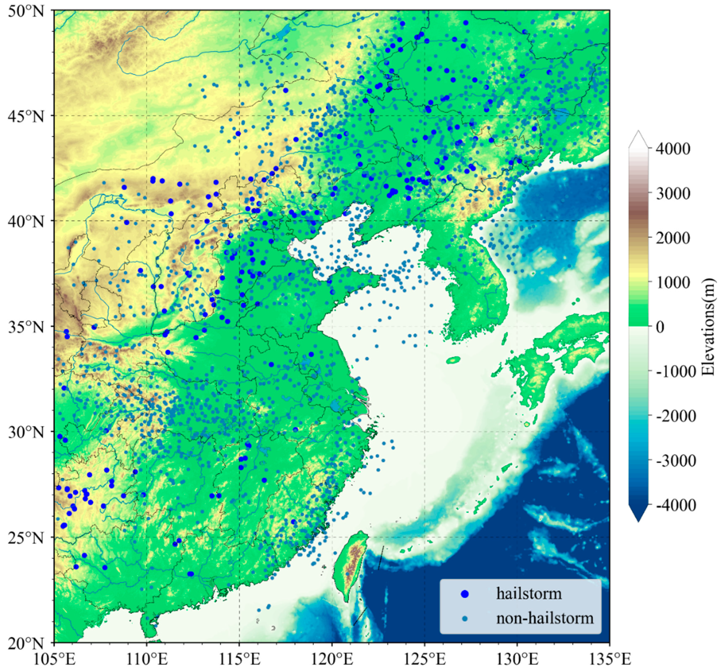
The geographical scope of the study, illustrated in Figure 1, extends from 20° to 50°N in latitude and 105° to 135°E in longitude. Three types of data were leveraged: satellite, reanalysis, and hail. Data from March to August 2018 were used to develop and validate the machine learning models due to the availability of reliable hail event records that are precise to the minute during this period. In contrast, data from March to August 2019 to 2023 were used for the statistical analysis of the spatial distribution of hail and comparative analysis as, during this period, only hail event records precise to the hour were available.

Figure 1.
Study area and sample distribution. Dark blue circles indicate hailstorm samples, while light blue circles denote non-hailstorm samples.
2.1.1. Satellite Data
- (a)
- FY-4A
The FY-4A satellite, positioned at 104.7°E longitude above the equator since 25 May 2017, was officially commissioned for use on 25 September 2017. The FY-4A satellite’s onboard Advanced Geostationary Radiation Imager (AGRI) is equipped with a total of 14 channels. It provides a spatial resolution ranging from 0.5 to 1 km in the visible/near-infrared band, and from 2 to 4 km in the infrared band. The full disk scan requires 15 min, whereas the scan for the China region takes approximately 5 min. For the development of an all-day hail detection model, this study exclusively uses the brightness temperature data from the six infrared bands at wavelengths of 6.25, 7.1, 8.5, 10.7, 12.0, and 13.5 µm.
- (b)
- GPM PF database
The Global Precipitation Measurement (GPM) [45] Mission Core Observatory satellite was launched on 27 February 2014. The satellite is equipped with instruments including the GPM Microwave Imager (GMI), a passive multi-channel conical-scanning microwave radiometer, and the Dual-frequency Precipitation Radar (DPR), which functions at 13.6 GHz (Ka band) and 35.5 GHz (Ku band). These instruments enable the global measurement of precipitation, ranging from light to heavy. Precipitation Features (PFs), as defined by Nesbitt et al. [46], consist of contiguous pixels meeting specific criteria derived from the swath data of the DPR or GMI. For example, this study uses a PF database known as ‘ku40dbzf’ [47,48,49], characterized by areas with Ku band reflectivity exceeding 40 dBZ within the column, which is within the normal swath of Ku. The parameters MIN19PCT and MIN37PCT are employed to define hail PFs, adhering to the methodologies outlined by Ni17, Mroz17, and CB12.
- (c)
- GPM Hail Climatology Data Products
The Passive Microwave Hail Climatology Data Products, as detailed by Cecil and Bang [50], offer gridded (2° × 2°) annual estimates of severe hailstorm frequency. These estimates are based on data from the GPM GMI. The hail probability for each feature is determined using the 37 GHz and 19 GHz PCT retrievals with the BC19 method. A feature is defined as a contiguous area exceeding the size of one GPM GMI pixel, with an 89-GHz PCT value below 200 K. Furthermore, features undergo a screening process to exclude surface artifacts and deep convection, as described by Bang and Cecil [16]. Subsequently, features with an estimated hailstorm probability of at least 20% are tallied within each 2-degree grid box.
2.1.2. Reanalysis Data
The fifth generation of ECMWF reanalysis, ERA5, integrates model data with observations via data assimilation for comprehensive global climate and weather analysis. The data have been re-gridded to a regular latitude–longitude grid with a 0.25-degree resolution. ERA5 provides hourly estimates across a wide range of variables, including atmospheric, oceanic, wave, and land-surface parameters. At varying pressure levels, seven key quantities are used to calculate environmental parameters: geopotential (m2 s−2), potential vorticity (K m2 kg−1 s−1), relative humidity (%), specific humidity (kg−1 kg−1), temperature (K), U-component of wind (m s−1), and V-component of wind (m s−1). These quantities are crucial for assessing parameters such as the Convective Available Potential Energy (CAPE), the height of 0 °C isotherm, 0–3 km vertical wind shear (VWS0–3), Storm-relative helicity (SRH), and the Lapse-rate tropopause (LRT), among others. Additionally, the single-level quantity of skin temperature is used to detect snow- and ice-covered surfaces, as discussed by Zhou et al. [51]. These surfaces can result in significantly low PCT values in the data retrievals, according to Ni17, Mroz17, and CB12 methodologies.
2.1.3. Hail Data
- (a)
- Hail Event Records
Hail events are routinely recorded at weather stations within China’s national surface meteorological observational network. Standard hail event records include latitude, longitude, date, exact time of occurrence (down to the hour and minute), and the maximum hailstone diameter. These records are measured or estimated by professionally trained meteorological observers in accordance with observational guidelines, ensuring that they are both detailed and reliable. Data from March to August 2018 were specifically used for training, validation, and testing of the machine learning models.
- (b)
- 1-h Hail Event Records
The other type of hail data used in this study consists of hourly hail event records, which include the latitude, longitude, date, and hour of hail occurrence. These hail event records are automatically captured by instruments and lack precise observation times (i.e., to the minute) and records of the maximum hailstone diameter. 1-h hail event records from March to August from 2019 to 2023 were utilized for the statistical analysis of the spatial distribution of hail occurrences, serving as a benchmark for comparing the various hail detection methods.
- (c)
- Direct Economic Losses
We also retrieved some data from the Yearbook of Meteorological Disasters in China to illustrate the direct economic losses caused by hail and other severe convective weather each year from 2012 to 2021, as shown in Table 1 [3,4,5,6,7,8,9,10,11,12].

Table 1.
Direct economic losses caused by hail, tornadoes, and other severe convective weather from 2012 to 2021.
2.2. Methods
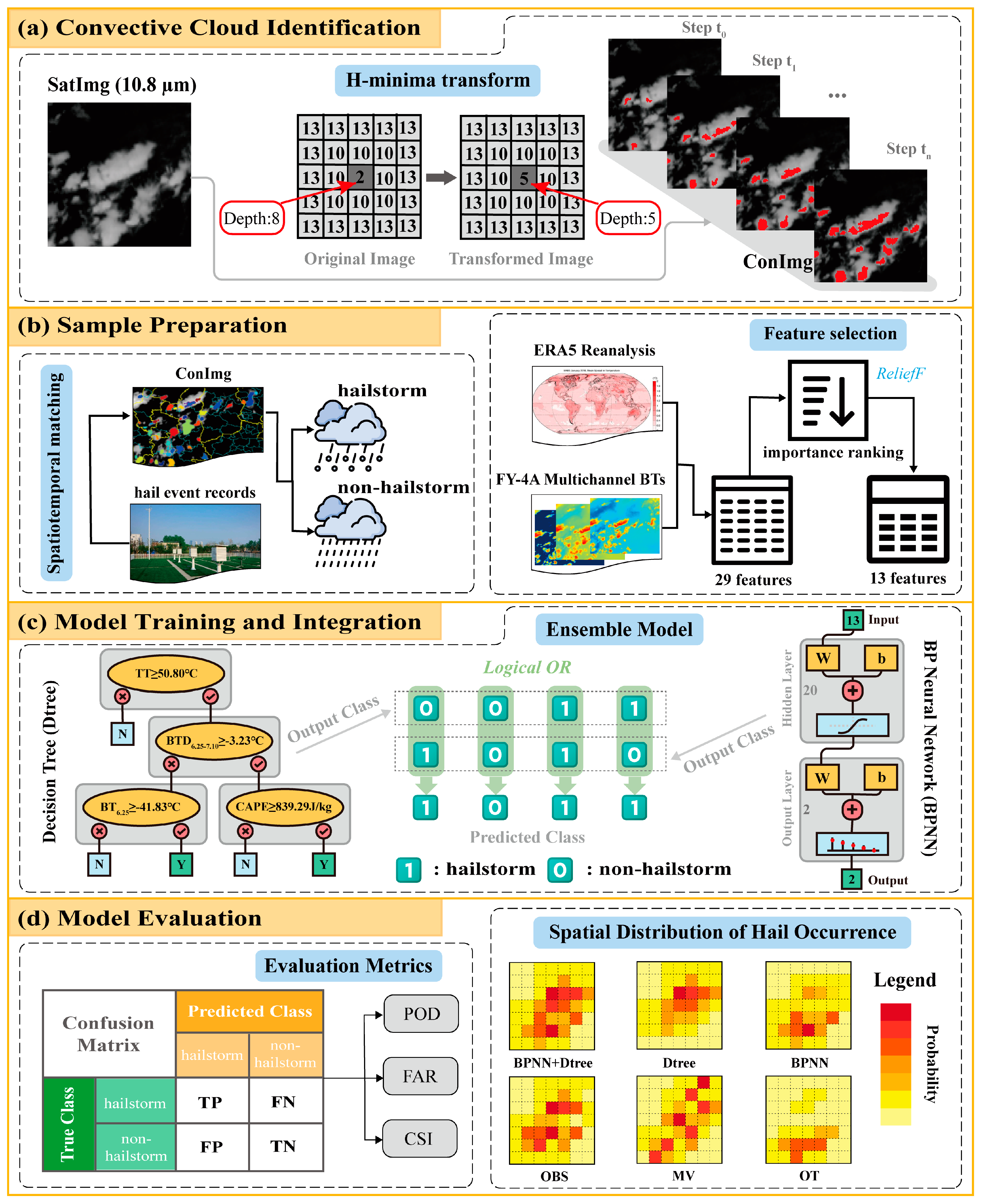
To detect hailstorms from satellite images, the initial step involves identifying convective clouds. Subsequently, an ensemble classifier—which is an ‘OR’ model combining a BP neural network and a decision tree—is constructed to determine whether the convective cloud is a hailstorm or not. The entire process is shown in Figure 2.

Figure 2.
Technical roadmap for developing an ensemble machine learning model for hailstorm identification.
- (a)
- Convective Cloud Identification
On satellite images, convective cloud (CC) areas frequently merge with other cloud regions, making it essential to isolate CCs before analyzing their physical properties. This study employs an iterative H-minima transform algorithm, as referenced in the work of Liu et al. (2014) [52], for this purpose. The algorithm includes five steps per iteration after assigning initial values, as shown in Figure 3a: (1) H-Minima Transform Execution—Conduct an H-minima transform on the satellite image (SatImg). For any connected region with a minimum brightness temperature , if the BT at any point within satisfies , where is the H-minima transform threshold (varying from to with an increase in ), then adjust to . Otherwise, retain the original . This process generates an image, which we denote as HImg. (2) Regional Minima Identification—On HImg, pinpoint regional minima and assign them a value of 1, while setting all other pixels to 0, creating a binary image denoted as BImg. (3) Connected Region Division—Segment the connected regions in BImg into distinct CC areas. (4) CC Image Update—For the convective cloud image (ConImg), if the threshold is less than (the merging threshold for CCs), set the value of ConImg for each CC (CCi) to 1. For greater than or equal to , calculate the intersection count between CCi and previously identified CCs. If the intersection count is less than 2, set the value of ConImg at CCi to 1. (5) Iteration Exit Criteria—Decide whether to conclude the iteration process. If exceeds , terminate the iteration to obtain the final ConImg, where each CCi denotes a recognized convective cloud. Figure 3b demonstrates several CC identification scenarios: CCA continues to expand outward with each iteration; CCB consists of two small CCs that merge into a single CC before ; and CCC and CCD, due to the two CCs not merging before , remain as two separate CCs in the end. The smaller the value of , the smaller the initial CC, leading to the identification of more CCs; conversely, the larger the value of , the larger the initial CC (merging more small CCs), resulting in fewer CCs identified in the end. The smaller the value of , the smaller the final CC obtained; the larger the value of , the larger the final CC, but it will no longer grow if the peripheral expansion intersects with other CCs. The value of determines the speed at which the CC expands outward, while determines whether it is permissible to merge two or more CCs identified in the previous iteration step into one cloud mass identified at this iteration. Merging is only allowed when . In this study, the values of , , , and were set as 1.0, 24, 0.1, and 2.0, respectively.
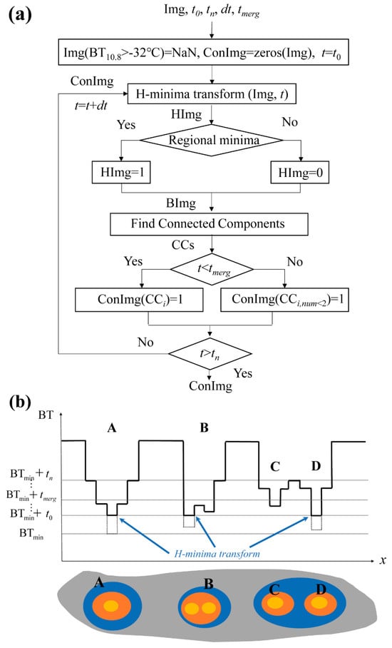
Figure 3.
(a) Flowchart of the iterative H-minima transform method for identifying convective clouds. (b) Schematic of the process for identifying convective clouds with the iterative H-minima transform method.
- (b)
- Sample Preparation
To correlate identified convective clouds (CCs) with hail observation records from meteorological stations between March and August 2018, we employed a spatial and temporal matching process. The matching criteria were as follows: the time difference with the hail observation must not exceed 5 min, there should be intersecting pixels within a 5 × 5 pixel window surrounding the station, and the CC with the shortest average distance to the station is designated as a hailstorm. Given that hail events are rare, in order to minimize the inclusion of non-hailstorm samples and concentrate on those with high similarity, non-hailstorm samples were selected from CCs at the same moment. However, these samples had to adhere to the criterion of having no hail observation records within a 100-pixel range around them within an hour. Through this matching process, we obtained a dataset comprising 221 hailstorm and 2271 non-hailstorm samples, as illustrated in Figure 1.
For each hailstorm and non-hailstorm sample, we calculated 29 physical quantities that are commonly referenced in the literature, as listed in Table 2. These quantities include cloud-top brightness temperature (BT), differences between brightness temperatures (BTD), and environmental thermodynamic and dynamic parameters. Detailed information about these quantities, their references, and their physical significance can be found in the work of Wu et al. [53]. To calculate the 29 physical quantities of hailstorms (non-hailstorms), the values at each pixel within the hailstorm (non-hailstorm) boundary were first estimated. The cloud-top BT/BTD for each pixel can be directly calculated from the satellite infrared channel observations, while the environmental thermodynamic and dynamic parameters for each pixel are derived from the corresponding ERA5 grid data at the pixel’s location. The final physical quantities are the average values across all pixels within a given bounded region.

Table 2.
Physical quantities calculated for each hailstorm (non-hailstorm) sample.
We utilized the ReliefF algorithm—as introduced by Kononenko et al. [54] and further developed by Robnik-Šikonja and Kononenko [55]—to rank the significance of these 29 physical quantities in distinguishing between hailstorm and non-hailstorm samples. The ReliefF algorithm allocates weights to features based on their capacity to differentiate samples that are in close proximity to one another within their respective classes. A higher weight indicates that the feature is more effective in distinguishing between the two categories. The ranking outcomes are presented in Figure 4, which reveals six distinct breakpoints in the weight distribution chart. For this study, we chose the breakpoint at the fourth division as the cutoff point. Consequently, we selected the top 13 features, as indicated by their ranking, to serve as input features for our machine learning model.
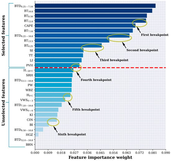
Figure 4.
Bar chart of feature importance ranking using the ReliefF method. Six distinct breakpoints are indicated by yellow ellipses. The red dashed line drawn at the fourth breakpoint serves as the cutoff point for this study; features with importance scores above this line (amounting to 13 features) were chosen as inputs for the model, whereas those with lower scores were excluded.
- (c)
- Model Training and Integration
The hailstorm and non-hailstorm samples were divided into three distinct groups: a training set, a validation set, and a test set, with respective proportions of 60%, 10%, and 30%. The training set served as the foundation for computing gradients and updating the weights and biases of the BP neural network (BPNN) model, following the principles outlined by Glorot and Bengio [56]. For the decision tree (Dtree) model, this dataset was instrumental in splitting tree nodes, continuing until the tree reaches its maximum depth or the number of samples in a node falls below a predefined threshold, as described by Loh [57]. The validation set plays a crucial role in identifying the optimal hyperparameters for the models and in curbing overfitting. In the case of the BPNN model, early stopping was implemented as a technique to prevent overfitting. For the Dtree model, the practice of pruning was applied with the same intent. During the model training for hyperparameter selection, grid search was primarily utilized. The selected hyperparameters included the Maximal Number of decision Splits (MaxNumSplits) and Minimum size of leaf node observations (MinLeafSize) for the Dtree model and Hidden Layer sizes (HLayersize) for the BPNN model. Furthermore, given the imbalance in the sample sizes between hailstorm and non-hailstorm samples, and recognizing the serious consequences of misclassifying a hailstorm as a non-hailstorm, we introduced the hyperparameter of Prior Probability (PP) for each class during Dtree model training. This adjustment in class weights reduces the model’s bias towards the majority class of non-hailstorms and enhances the detection rate of the minority class of hailstorms. Additionally, when training the BPNN model, a hyperparameter of Error Weights (EW) for each class was incorporated. This assigns a higher weight to the error of misidentifying a hailstorm as a non-hailstorm and a lower weight to the reverse misidentification, thus aligning the model’s outputs with the severity of different misclassification scenarios. The search range and values of the hyperparameters are presented in Table 3. The test set was reserved for the evaluation of model performance, as detailed in step (d).

Table 3.
The hyperparameters of the Dtree and BPNN models.
The architecture of the trained Dtree and BPNN models are depicted in Figure 2c. The Dtree model was structured with a single root node (), one internal node in the first layer (), two internal nodes in the second layer ( and ), and five leaf nodes, which use Yes (Y) or No (N) to indicate whether the final decision is a hailstorm. The BPNN model was designed with a two-layer fully connected architecture, which includes one hidden layer comprising twenty neurons and one output layer with two neurons. The hyperbolic tangent function was used as the activation function of the hidden layer, and the model adopted the cross-entropy loss function.
To bolster the identification of hail hazards, which can be challenging for machine learning models due to their minority class status, an ensemble approach using the logical ‘OR’ operation to combine the BPNN and Dtree models is proposed, denoted as BPNN+Dtree. Specifically, for any given CC sample, if either the Dtree or the BPNN model predicts it as a hailstorm (assigned a value of 1), the sample is classified as a hailstorm. On the other hand, the sample is classified as a non-hailstorm (assigned a value of 0) only if both models concur on this classification, as depicted in Figure 2c. As the integration is performed on the classification results (not the output probabilities) of the two models, there are only two methods: ‘OR’ and ‘And’. When the ‘And’ method is used, a sample is considered a hailstorm only if both models identify it as such. However, hailstorms, on one hand, are not easily detected by machine learning models due to their nature as rare occurrences. On the other hand, hail is hazardous weather, and the risk of failing to predict a hailstorm is much greater than that of issuing a false alarm. Therefore, the aim is to identify as many hailstorms as possible. Therefore, based on these two considerations, this study employed the ‘OR’ method for integration.
- (d)
- Model Evaluation
The model evaluation focused on two main aspects, as shown in Figure 2d. The first aspect involved calculating key evaluation metrics, including POD, FAR, and CSI, all of which were derived from the confusion matrix of the test set. The respective calculation formulas are as follows:
Here, TP (True Positive) denotes the number of samples correctly identified as the hail class, FP (False Positive) is the number of samples incorrectly classified as the hail class when they do not belong to it, FN (False Negative) is the number of hail samples that were incorrectly classified as non-hail, and TN (True Negative) is the number of non-hail samples correctly identified.
The evaluation also included a statistical comparison of the spatial distribution characteristics of hail occurrences, organized into three comparative groups: (1) A comparative analysis of different machine learning models, including the BPNN, Dtree, and BPNN+Dtree models; (2) the ensemble model BPNN+Dtree was compared with the OT and OTfilter hail identification methods; and (3) the ensemble model BPNN+Dtree was also compared with various microwave-based hail identification methods—namely, Ni17, CB12, Mroz17, and BC19. Each hail identification method identifies different objects: machine learning models classify CCs, OT-based methods analyze cloud pixels, and microwave-based methods detect PFs. Additionally, the temporal scope of the statistical analysis varies. The statistical period for machine learning models and OT-based methods spans from 2019 to 2023, while microwave-based methods cover a longer period from 2014 to 2023. This extended period for microwave-based methods is necessary due to the polar orbit of the GPM satellite, which restricts the visibility of spatial distribution characteristics when observed over shorter durations. To standardize the comparison, the hail occurrences were tallied within each 2° × 2° grid cell. Specifically, for the machine learning models, the number of hailstorm center points falling within each grid cell was counted; for the OT-based method, the number of hail cloud pixels falling within each grid cell was calculated; and, for microwave-based methods, the number of hail PFs center points falling within each grid cell was accumulated. These counts were then normalized through dividing them by the total number of hail occurrences, thereby converting the raw counts into probabilities for further analysis.
3. Results
3.1. Results of Convective Cloud Identification
Figure 5a–h depict the results of the iterative H-minima transform method for identification of CCs on the FY-4A 10.8-µm infrared image at 06:38 UTC on 11 August 2018. As the process unfolds, it can be observed that the area of the identified CCs progressively expands with each iteration, as shown in Figure 5a–h. The final identification result is presented in Figure 5h, where different colors represent distinct CCs. At this stage, the area of each CC either ceases to grow or, if it continues to expand, it merges with other CCs. This highlights the dynamic nature of the identification process and the method’s effectiveness in delineating CCs.
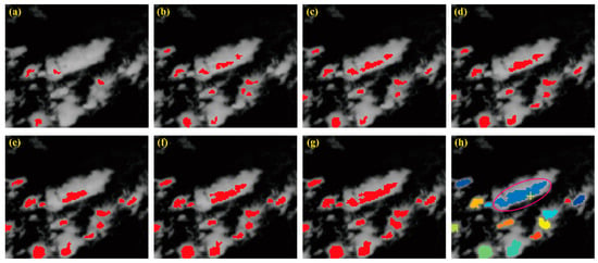
Figure 5.
The results of the identification of convective clouds using the iterative H-minima transform method on the FY-4A 10.8-μm infrared channel image, recorded at 06:38 UTC on 11 August 2018. (a–h) illustrate the outputs at various time steps throughout the process. In (h), the identified convective clouds are differentiated by color, with yellow plus signs indicating the positions of observed hail, and magenta ellipses outlining the corresponding hailstorms.
3.2. Statistical Results of Selected and Unselected Features
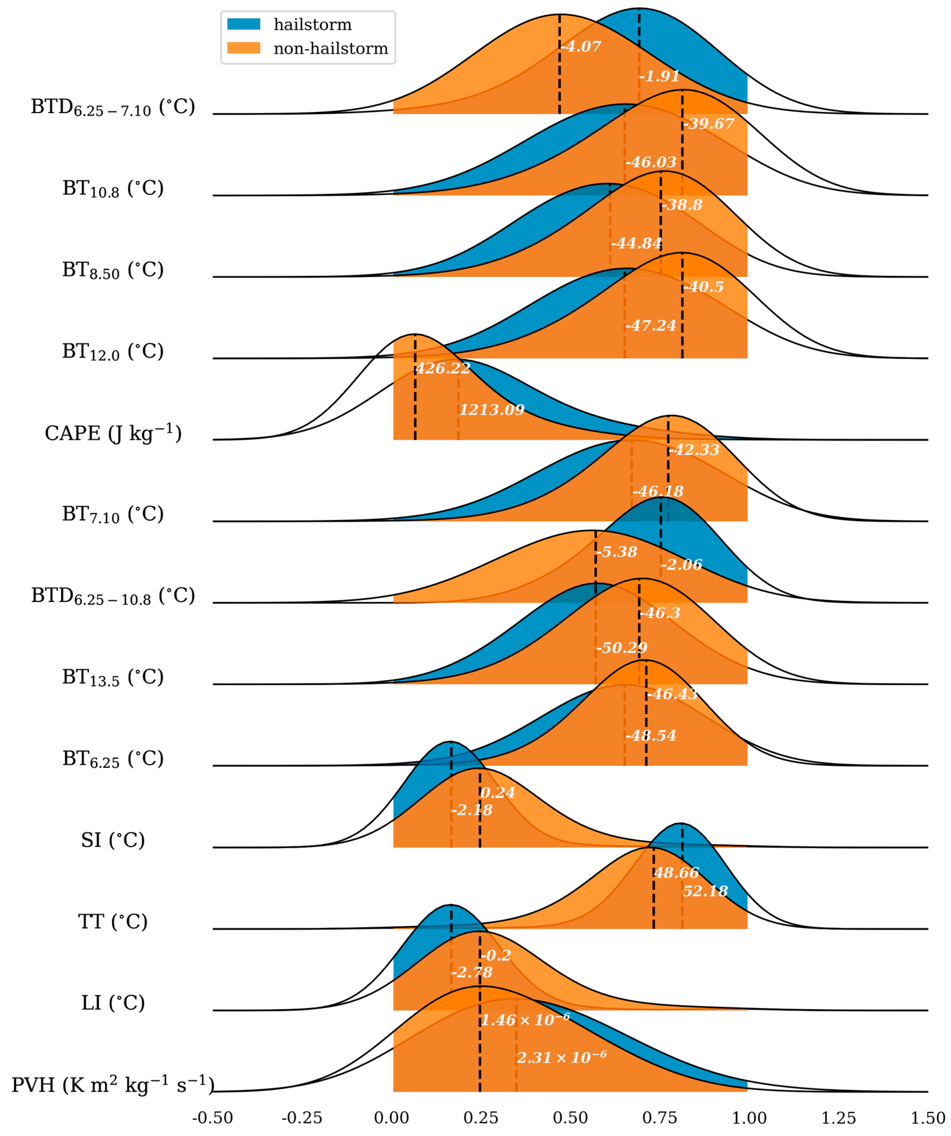
To validate the feature selection, joy plots for both selected and unselected features were created, as shown in Figure 6 and Figure 7. The blue and orange curves in these figures represent the Gaussian kernel density estimation for the hailstorm and non-hailstorm classes, respectively. Figure 6 demonstrates a clear distinction between the joy plots of hailstorms and non-hailstorms, characterized by distant peaks and distinctly different curve shapes. In contrast, Figure 7 reveals a significant overlap in the joy plots for both classes, with centers and curve shapes showing various degrees of overlap.

Figure 6.
Joy plot of selected features. The curve filled with blue color represents the Gaussian kernel density estimation for hailstorm samples, while the orange curve represents the same for non-hailstorm samples. The horizontal axis represents the normalized value of each feature’s physical quantity. The black dashed line marks the feature value where the probability density is at its maximum. The white numbers correspond to the actual physical values.
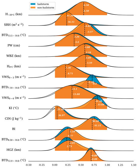
Figure 7.
Joy plot for unselected features. Similar to Figure 6, this plot presents the Gaussian kernel density estimation curves for hailstorm and non-hailstorm samples, but for features that were not selected.
The results suggest that the selected features offer a more discernible differentiation between hailstorms and non-hailstorms than the unselected features, making them more rational for use. The selected features mainly encompass physical quantities that reflect cloud-top characteristics, such as height, thickness, and water vapor distribution (e.g., BTD6.25–7.10, BT6.25), as well as thermodynamic conditions (e.g., CAPE, TT). Dynamic factors such as VWS0–3 and SRH were not selected. This selection deviates from previous criteria for hail intensity classification, which prioritized physical quantities related to cloud-top height, dynamic properties, and melting level height, including vertical wind shear, a factor known for its strong correlation with large hail events [53].
3.3. Confusion Matrix Evaluation Results
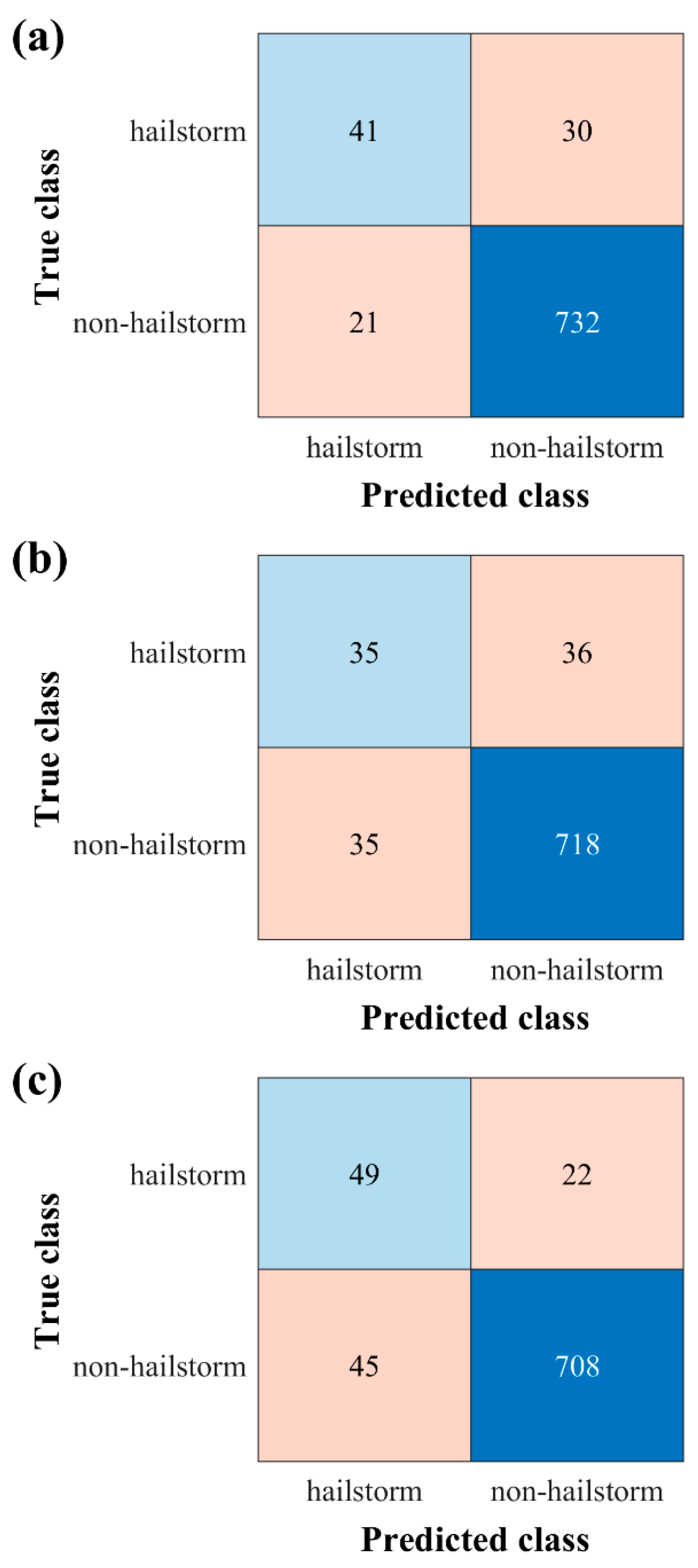
To assess the model’s predictive performance, confusion matrices for the BPNN, Dtree, and BPNN+Dtree models were constructed for the test set, as shown in Figure 8. The evaluation metrics POD, FAR, and CSI were computed and presented in Table 4. From Figure 8, it can be seen that through addressing the sample imbalance issue, the detection rate of hailstorms (minority class) with the three models improved, rather than obtaining a high overall accuracy rate () by tendentiously identifying all samples as non-hailstorms (majority class). Table 4 illustrates that the BPNN model consistently outperformed the Dtree model across all evaluated metrics: POD, FAR, and CSI. Notably, the ensemble model BPNN+Dtree had significantly improved POD (reaching 0.69), compared to the individual models. Meanwhile, its FAR value was between those of the BPNN and Dtree models. This indicates that the BPNN+Dtree model achieved a balance that effectively increases the POD for hailstorms without causing a substantial increase in the FAR.
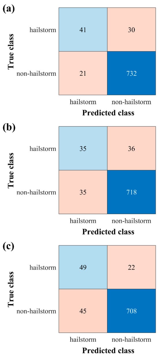
Figure 8.
Confusion matrices for various models on the test set. (a) BPNN; (b) Dtree; (c) BPNN+Dtree.

Table 4.
Performance metrics (POD, FAR, and CSI) of different classification machine learning models on the test set.
3.4. Statistical Results of Hail Occurrence Probability Spatial Distribution
3.4.1. Dtree vs. BPNN vs. BPNN+Dtree vs. OBS
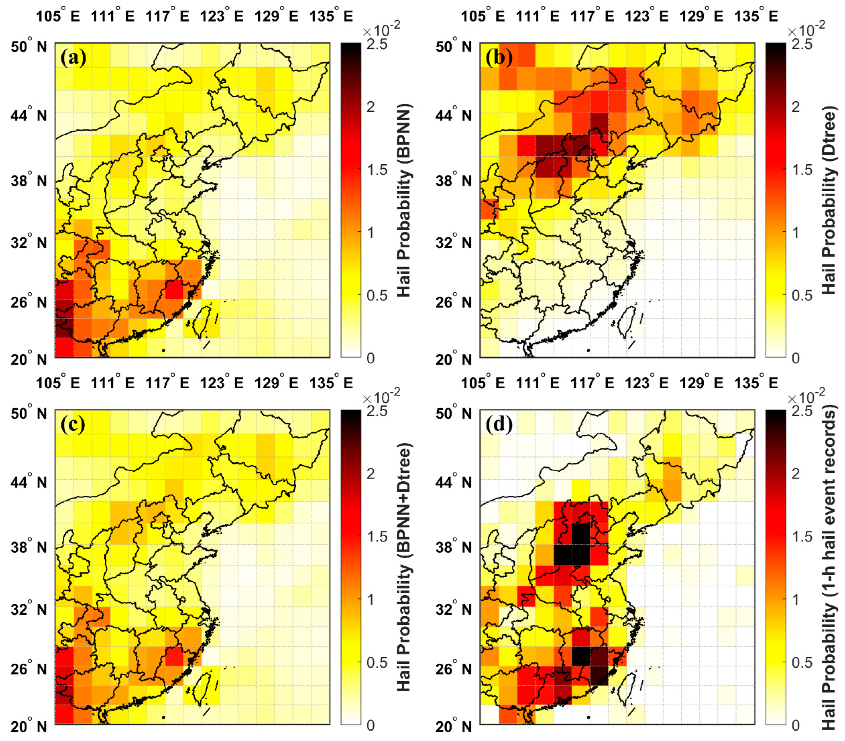
Figure 9a–c presents the spatial distribution of hail occurrence probability calculated based on hailstorms identified from 2019 to 2023 with the three distinct machine learning models. Specifically, Figure 9a illustrates the results for the BPNN model, Figure 9b shows those for the Dtree model, and Figure 9c shows those for the BPNN+Dtree ensemble model. For reference, Figure 9d depicts the spatial distribution derived from 1-h hail event records within the same period.
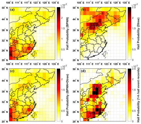
Figure 9.
Spatial distribution of hail occurrence probability calculated using various machine learning models: (a) The BPNN model; (b) the Dtree model; (c) the BPNN+Dtree ensemble model; and (d) 1-h hail event records.
The BPNN model (Figure 9a) presented a closer match to the observational data (Figure 9d) in terms of spatial distribution characteristics than the Dtree model (Figure 9b). Both the BPNN and observational calculations identified three high-frequency hail regions: the southeast coastal area, North China, and Northeast China. However, the BPNN model was more effective in identifying hail in the southern regions while performing relatively poorly for northern hail. In contrast, the Dtree model was more sensitive to hail in the northern regions. The BPNN+Dtree ensemble model (Figure 9c) capitalizes on the strengths of both, enhancing the detection capability for hail across the entire region and providing a more accurate spatial distribution of hail probability that closely mirrors the observations. However, as the number of hailstorms identified by the Dtree model was much smaller than that identified by the BPNN model, the BPNN+Dtree ensemble model still had a relatively low probability in the north. Additionally, the machine learning models analyzed hailstorms using satellite infrared images, while the observational data were reliant upon on-site observations. This discrepancy explains the broader spatial distribution range evident in Figure 9a–c, compared to the more focused distribution in Figure 9d.
3.4.2. BPNN+Dtree vs. OT vs. OTfilter vs. OBS
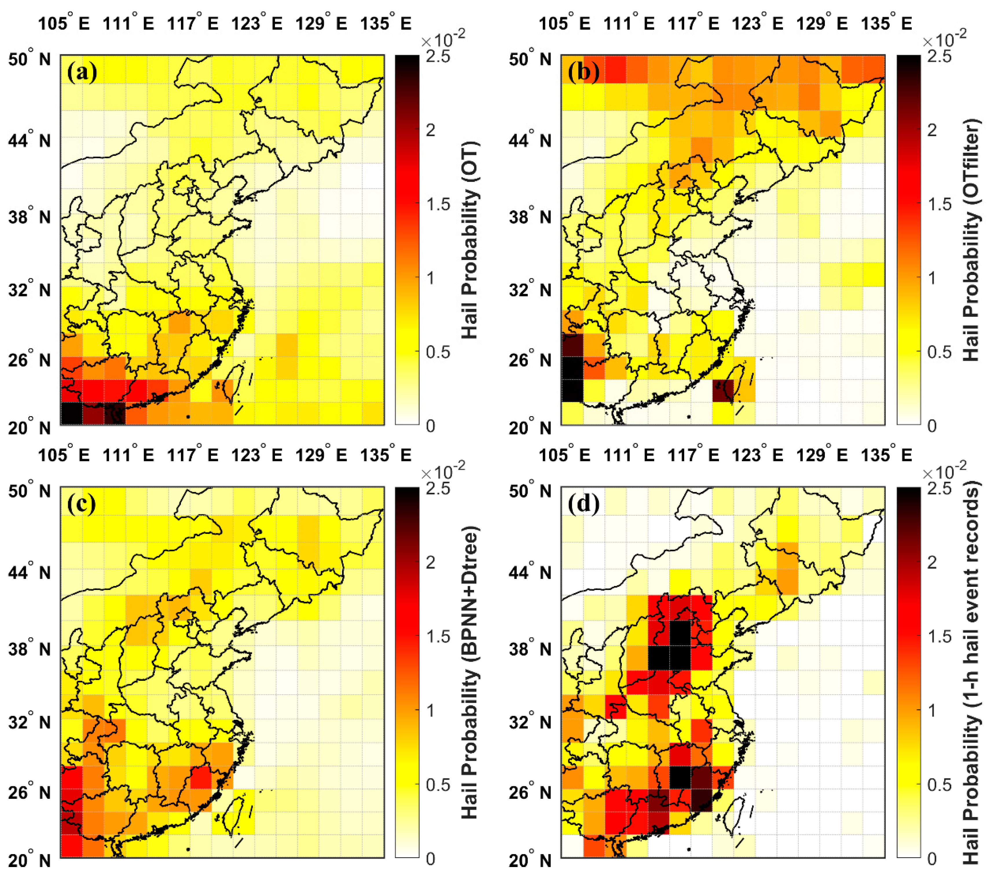
The spatial distribution of hail occurrence probability calculated based on hail cloud pixels identified by the OT method was predominantly concentrated in the tropical region, as shown in Figure 10a. However, when environmental filtering factors were taken into account, the identification results obtained with the OTfilter method were skewed towards the overly northern region. This suggests that the applicability of both the OT and OTfilter methods is relatively limited in the China region. In contrast, the result of the BPNN+Dtree ensemble model presented in Figure 10c, showed a significantly higher degree of congruence with the 1-h hail event records depicted in Figure 10d. The above comparative results indicate that the BPNN+Dtree model has stronger applicability over China.

Figure 10.
Comparison of the spatial distribution of hail occurrence probability obtained with the BPNN+Dtree ensemble model and OT-based hail identification methods: (a) Calculated based on hail cloud pixels identified by the OT method; (b) calculated based on hail cloud pixels identified by the OTfilter method; (c) calculated using the BPNN+Dtree ensemble model-identified hailstorms; (d) calculated based on 1-h hail event records.
3.4.3. BPNN+Dtree vs. Ni17 vs. Mroz17 vs. CB12 vs. BC19 vs. OBS
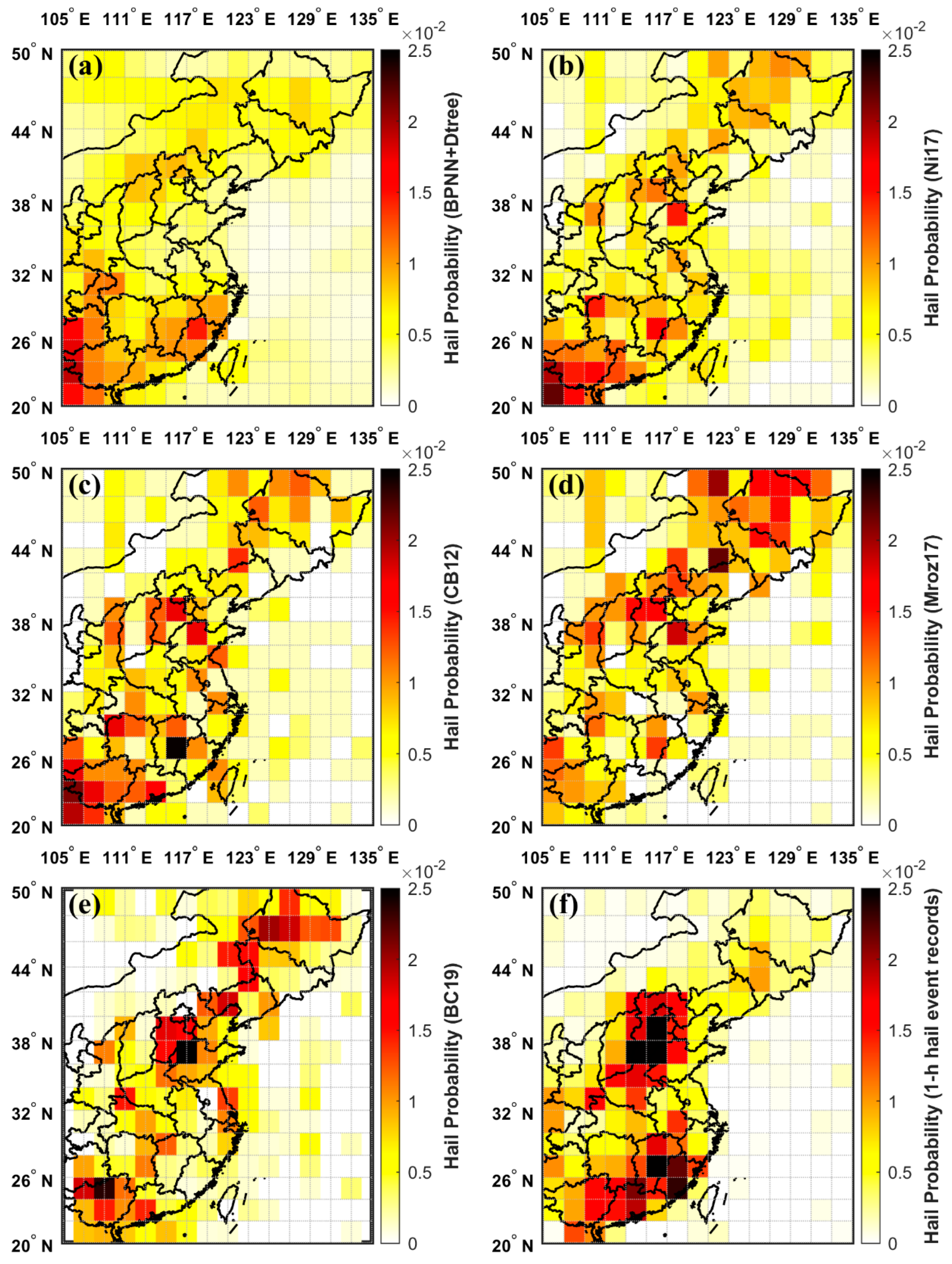
Figure 11b–e depict the spatial distributions of hail occurrence probability as determined using the microwave-based methods Ni17, Mroz17, and CB12, as well as the reference method BC19. No high-frequency centers were evident, but a clear belt of hail occurrences stretches from the northeast to the southwest, aligning with the boundary of the subtropical high. The distribution pattern of the BPNN+Dtree ensemble model, as shown in Figure 11a, closely aligns with those of the Ni17 and BC19 methods. The model’s three high-frequency areas are located on this belt, sequentially forming from south to north. This formation is due to the northward shift of the monsoon rain belt, which follows the northward movement of the subtropical high. It can be seen that the hail distribution characteristics delineated by the BPNN+Dtree ensemble model are in accordance with the actual climatic patterns.
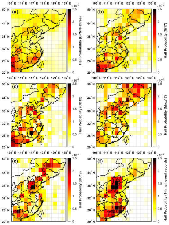
Figure 11.
Comparison of the spatial distribution of hail occurrence probability obtained with the BPNN+Dtree ensemble model and microwave-based hail identification methods: (a) Calculated using the BPNN+Dtree ensemble model-identified hailstorms; (b) calculated using the Ni17 method-identified hail PFs; (c) Calculated using the CB12 method-identified hail PFs; (d) calculated using the Mroz17 method-identified hail PFs; (e) calculated based on the published BC19 annual average data; and (f) calculated based on 1-h hail event records.
4. Discussion
This study utilizes FY4A satellite data and ensemble learning models to identify hailstorms in China, thus improving the accuracy of real-time monitoring and early warning systems for hail disasters.
The study began by employing the H-minima transform method to identify CCs, which are then correlated with the hail event records from March to August 2018. This process resulted in the collection of 221 hailstorm samples and 2271 non-hailstorm samples. For each sample, 29 features were calculated, encompassing cloud-top BT (BTD), thermodynamic, and dynamic features. The ReliefF method was then applied to filter these features, leading to the selection of 13 input features that can effectively distinguish between hailstorms and non-hailstorms. A comparative joy plot analysis of the selected versus unselected features revealed that the Gaussian kernel density curves of the selected features showed a greater degree of separation between the two sample types, indicating their superior discriminative power. From a physical perspective, the preferred quantities for classifying hailstorms are those that reflect cloud-top characteristics such as height, thickness, and water vapor distribution (e.g., BTD6.25–7.10 and BT6.25), as well as thermodynamic conditions such as CAPE and TT. In contrast, for the estimation of hail intensity, the focus is on cloud-top height and dynamic features, such as wind shear, which is a strong indicator of large hail events [53].
Next, Dtree and BPNN models were trained for the classification of hailstorms and non-hailstorms, using prior probability and error weight hyperparameters to improve the detection rate of the hailstorm class (minor class) and using pruning and early stopping techniques to mitigate overfitting. Given the higher risk associated with failing to report hail events compared to the risk of false alarms, the outputs of the Dtree and BPNN models were integrated using a logical ‘OR’ operation; therefore, the ensemble model—termed BPNN+Dtree—predicts a hailstorm if either model outputs a positive result. The BPNN+Dtree model achieved a POD value of 0.69 on the test set, which is significantly higher than those of the BPNN model (0.58) and the Dtree model (0.49), with an FAR balanced between those of the two models.
To evaluate the long-term identification effectiveness of the BPNN+Dtree model, a statistical analysis of hailstorms identified by the BPNN+Dtree ensemble model from 2019 to 2023 was conducted. The spatial distribution of hail occurrence probability was compared with the results obtained with other methods, including individual Dtree and BPNN models, OT-based identification methods, and microwave-based identification methods. The analysis revealed that the Dtree model is more likely to identify northern hailstorms, while the BPNN model is more likely to identify southern hailstorms. As such, the integration of these two models into the BPNN+Dtree model improved its identification capability across the whole of China. The three high-incidence areas of hail identified—namely, the southeast coastal region, North China, and Northeast China—were in close agreement with observational data. In contrast, the OT-based hail identification method calculated hail high-frequency areas that significantly deviated from the observed patterns tending to concentrate in tropical regions or the northern areas, making it less suitable for hail detection in China. The spatial distribution of hail occurrence probability calculated using the microwave-based methods presented no obvious high-frequency centers. Instead, a northeast–southwest belt distribution was observed, which aligns with the direction of the subtropical high’s edge. The hail high-frequency areas calculated with the BPNN+Dtree ensemble model were also located on this belt, forming in sequence from south to north corresponding to the northward shift of the monsoon rain belt following the northward movement of the subtropical high.
Although the above results indicate that this study has established a relatively effective hailstorm detection model based on satellite data using ensemble machine learning methods, there are still aspects that can be further improved. First, the number of hailstorm samples should be increased. Typically, for machine learning models, the more and richer the training samples, the better the generalization performance of the model. Due to the lack of precise, minute-level reliable hail event records after 2018, the current work only used data from 2018 for training, which is insufficient for establishing a model with strong generalization capabilities. In the future, we plan to combine disaster records, radar observations, and other multi-source data to manually create more reliable hailstorm samples. This will be used for training more sophisticated models, thus improving the accuracy of hail identification. Second, although the ensemble method improved upon the predictive performance of the individual models, to a certain extent, the final results still presented a certain gap with respect to the observations, especially in the identification of hail in the northern regions, which requires further improvement. Based on increasing the training data, leading to improvement of the detection performance of individual models, the ensemble model can be expected to also perform better. Third, the logical ‘OR’ operation was used for model ensembling, which is suitable for models where the output is categorical (such as the Dtree model). In the future, if the output consists of probabilities for each class, alternative ensemble strategies such as averaging the probabilities, applying a voting mechanism, or selecting the maximum value could be explored, which is a more mathematical approach. Additionally, the number of models in the ensemble can be increased beyond the two considered here. When selecting models for integration, it is important to consider not only the accuracy but also the unique advantages of different models, such as their performance in different spatial areas or periods. This can mitigate the shortcomings of the integrated model and enhance its overall capabilities.
5. Conclusions
In summary, the proposed ensemble model BPNN+Dtree not only increased the hailstorm detection rate but also improved the overall detection accuracy using data from across China through combining the strengths of both models. For other types of hazardous weather besides hail, the risk of missed reports often exceeds that of false alarms, especially in the context of unbalanced samples where such weather events are rare. An integrated learning model can improve the detection rate while ensuring that the false alarm rate does not increase significantly.
Hailstorms, as a mesoscale weather phenomenon, are always considered to be unpredictable. To date, most automatic recognition methods for hailstorms have been developed based on radar echoes, while few take satellite observations into account. The ensemble machine learning model established in this study provides a method for hailstorm detection using satellite data, enabling large-scale automatic monitoring of hail, which contributes to improving the accuracy, timeliness, and refinement level of hail nowcasting and forecasting.
Author Contributions
Conceptualization, Q.W., Y.-X.S., Y.-G.Z., F.W. and C.-Y.W.; Methodology, Q.W. and Y.-X.S.; Validation, Q.W.; Formal analysis, Q.W.; Investigation, Q.W.; Resources, Q.W., Y.-X.S., Y.-G.Z. and F.W.; Data curation, Q.W., Y.-X.S. and Y.-G.Z.; Writing—original draft, Q.W.; Writing—review & editing, Q.W., Y.-X.S., Y.-G.Z. and C.-Y.W.; Visualization, Q.W.; Funding acquisition, Q.W., Y.-X.S. and F.W. All authors have read and agreed to the published version of the manuscript.
Funding
This research was funded by the National Natural Science Foundation of China (grant number 42375140 and 41965001) and the Key Project of the Science and Technology Commission of Shanghai Municipality (grant number 22DZ1100803).
Data Availability Statement
The FY-4A AGRI L1 data were obtained from the National Satellite Meteorological Center (NSMC) of the China Meteorological Administration (CMA), accessible at http://satellite.nsmc.org.cn/PortalSite/Default.aspx (accessed between the years 2018 and 2023). The GPM Precipitation Feature (PF) data were sourced from the Texas A&M University at Corpus Christi (TAMU-CC) precipitation feature database, available at http://atmos.tamucc.edu/trmm/data/ (accessed on 13 May 2024). The GPM Hail Climatology Data Products were retrieved from the NASA Earth Science Data Systems (ESDS) Program, found at https://search.earthdata.nasa.gov/search/granules?p=C2196515446-GHRC_DAAC&pg[0][v]=f&pg[0][gsk]=-start_date&q=hail&tl=1722849455!3!! (accessed on 25 April 2024). The ERA5 reanalysis data were downloaded from the Climate Data Store (CDS), which can be accessed at https://cds.climate.copernicus.eu/cdsapp#!/home (accessed between the years 2020 and 2023). Hail event records were collected from the National Meteorological Information Center (NMIC) of CMA. Additionally, the elevation data were obtained from Natural Earth, available at https://www.naturalearthdata.com/downloads/10m-natural-earth-1/10m-natural-earth-1-with-shaded-relief-and-water/ (accessed on 9 December 2020).
Acknowledgments
We express our gratitude to all these organizations for their outstanding work in data collection and production.
Conflicts of Interest
The authors declare no conflict of interest.
References
- Hand, W.H.; Cappelluti, G. A global hail climatology using the UK Met Office convection diagnosis procedure (CDP) and model analyses. Meteorol. Appl. 2011, 18, 446–458. [Google Scholar] [CrossRef]
- Zhang, X.; Sun, J.; Zheng, Y.; Zhang, Y.; Ma, R.; Yang, X.; Zhou, K.; Han, X. Progress in Severe Convective Weather Forecasting in China since the 1950s. J. Meteorol. Res. 2020, 34, 699–719. [Google Scholar] [CrossRef]
- Chinese Meteorological Administration. Yearbook of Meteorological Disasters in China; China Meteorological Press: Beijing, China, 2013. (In Chinese) [Google Scholar]
- Chinese Meteorological Administration. Yearbook of Meteorological Disasters in China; China Meteorological Press: Beijing, China, 2014. (In Chinese) [Google Scholar]
- Chinese Meteorological Administration. Yearbook of Meteorological Disasters in China; China Meteorological Press: Beijing, China, 2015. (In Chinese) [Google Scholar]
- Chinese Meteorological Administration. Yearbook of Meteorological Disasters in China; China Meteorological Press: Beijing, China, 2016. (In Chinese) [Google Scholar]
- Chinese Meteorological Administration. Yearbook of Meteorological Disasters in China; China Meteorological Press: Beijing, China, 2017. (In Chinese) [Google Scholar]
- Chinese Meteorological Administration. Yearbook of Meteorological Disasters in China; China Meteorological Press: Beijing, China, 2018. (In Chinese) [Google Scholar]
- Chinese Meteorological Administration. Yearbook of Meteorological Disasters in China; China Meteorological Press: Beijing, China, 2019. (In Chinese) [Google Scholar]
- Chinese Meteorological Administration. Yearbook of Meteorological Disasters in China; China Meteorological Press: Beijing, China, 2020. (In Chinese) [Google Scholar]
- Chinese Meteorological Administration. Yearbook of Meteorological Disasters in China; China Meteorological Press: Beijing, China, 2021. (In Chinese) [Google Scholar]
- Chinese Meteorological Administration. Yearbook of Meteorological Disasters in China; China Meteorological Press: Beijing, China, 2022. (In Chinese) [Google Scholar]
- Punge, H.J.; Kunz, M. Hail observations and hailstorm characteristics in Europe: A review. Atmos. Res. 2016, 176, 159–184. [Google Scholar] [CrossRef]
- Witt, A.; Eilts, M.D.; Stumpf, G.J.; Johnson, J.T.; Mitchell, E.D.; Thomas, K.W. An enhanced hail detection algorithm for the WSR-88D. Weather Forecast. 1998, 13, 286–303. [Google Scholar] [CrossRef]
- Wang, P.; Shi, J.; Hou, J.; Hu, Y. The Identification of Hail Storms in the Early Stage Using Time Series Analysis. J. Geophys. Res.-Atmos. 2018, 123, 929–947. [Google Scholar] [CrossRef]
- Bang, S.D.; Cecil, D.J. Testing Passive Microwave-Based Hail Retrievals Using GPM DPR Ku-Band Radar. J. Appl. Meteorol. Climatol. 2021, 60, 255–271. [Google Scholar] [CrossRef]
- Cecil, D.J. Passive Microwave Brightness Temperatures as Proxies for Hailstorms. J. Appl. Meteorol. Climatol. 2009, 48, 1281–1286. [Google Scholar] [CrossRef]
- Ni, X.; Liu, C.; Cecil, D.J.; Zhang, Q. On the Detection of Hail Using Satellite Passive Microwave Radiometers and Precipitation Radar. J. Appl. Meteorol. Climatol. 2017, 56, 2693–2709. [Google Scholar] [CrossRef]
- Mroz, K.; Battaglia, A.; Lang, T.J.; Cecil, D.J.; Tanelli, S.; Tridon, F. Hail-Detection Algorithm for the GPM Core Observatory Satellite Sensors. J. Appl. Meteorol. Climatol. 2017, 56, 1939–1957. [Google Scholar] [CrossRef]
- Cecil, D.J.; Blankenship, C.B. Toward a Global Climatology of Severe Hailstorms as Estimated by Satellite Passive Microwave Imagers. J. Clim. 2012, 25, 687–703. [Google Scholar] [CrossRef]
- Bang, S.D.; Cecil, D.J. Constructing a Multifrequency Passive Microwave Hail Retrieval and Climatology in the GPM Domain. J. Appl. Meteorol. Climatol. 2019, 58, 1889–1904. [Google Scholar] [CrossRef]
- Punge, H.J.; Bedka, K.M.; Kunz, M.; Werner, A. A new physically based stochastic event catalog for hail in Europe. Nat. Hazards 2014, 73, 1625–1645. [Google Scholar] [CrossRef]
- Bedka, K.; Brunner, J.; Dworak, R.; Feltz, W.; Otkin, J.; Greenwald, T. Objective Satellite-Based Detection of Overshooting Tops Using Infrared Window Channel Brightness Temperature Gradients. J. Appl. Meteorol. Climatol. 2010, 49, 181–202. [Google Scholar] [CrossRef]
- Bedka, K.M. Overshooting cloud top detections using MSG SEVIRI Infrared brightness temperatures and their relationship to severe weather over Europe. Atmos. Res. 2011, 99, 175–189. [Google Scholar] [CrossRef]
- Adler, R.F.; Markus, M.J.; Fenn, D.D. Detection of severe midwest thunderstorms using geosynchronous satellite data. Mon. Weather Rev. 1985, 113, 769–781. [Google Scholar] [CrossRef]
- Dworak, R.; Bedka, K.; Brunner, J.; Feltz, W. Comparison between GOES-12 Overshooting-Top Detections, WSR-88D Radar Reflectivity, and Severe Storm Reports. Weather Forecast. 2012, 27, 684–699. [Google Scholar] [CrossRef]
- Marion, G.; Trapp, R.J.; Nesbitt, S.W. Using overshooting top area to discriminate potential for large, intense tornadoes. Geophys. Res. Lett. 2019, 46, 12520–12526. [Google Scholar] [CrossRef]
- Punge, H.J.; Bedka, K.M.; Kunz, M.; Reinbold, A. Hail frequency estimation across Europe based on a combination of overshooting top detections and the ERA-INTERIM reanalysis. Atmos. Res. 2017, 198, 34–43. [Google Scholar] [CrossRef]
- Merino, A.; Lopez, L.; Sanchez, J.L.; Garcia-Ortega, E.; Cattani, E.; Levizzani, V. Daytime identification of summer hailstorm cells from MSG data. Nat. Hazards Earth Syst. Sci. 2014, 14, 1017–1033. [Google Scholar] [CrossRef]
- Melcón, P.; Merino, A.; Luis Sanchez, J.; Lopez, L.; Hermida, L. Satellite remote sensing of hailstorms in France. Atmos. Res. 2016, 182, 221–231. [Google Scholar] [CrossRef]
- Bergen, K.J.; Johnson, P.A.; de Hoop, M.V.; Beroza, G.C. Machine learning for data-driven discovery in solid Earth geoscience. Science 2019, 363, eaau0323. [Google Scholar] [CrossRef] [PubMed]
- Bonavita, M.; Arcucci, R.; Carrassi, A.; Dueben, P.; Geer, A.J.; Le Saux, B.; Longepe, N.; Mathieu, P.-P.; Raynaud, L. Machine Learning for Earth System Observation and Prediction. Bull. Am. Meteorol. Soc. 2021, 102, E710–E716. [Google Scholar] [CrossRef]
- Dramsch, J.S. 70 years of machine learning in geoscience in review. Adv. Geophys. 2020, 61, 1–55. [Google Scholar] [CrossRef]
- Fleming, S.W.; Watson, J.R.; Ellenson, A.; Cannon, A.J.; Vesselinov, V.C. Machine learning in Earth and environmental science requires education and research policy reforms. Nat. Geosci. 2021, 14, 878–880. [Google Scholar] [CrossRef]
- Im, J.; Park, H.; Takeuchi, W. Advances in Remote Sensing-Based Disaster Monitoring and Assessment. Remote Sens. 2019, 11, 2181. [Google Scholar] [CrossRef]
- Karpatne, A.; Ebert-Uphoff, I.; Ravela, S.; Babaie, H.A.; Kumar, V. Machine Learning for the Geosciences: Challenges and Opportunities. Ieee Trans. Knowl. Data Eng. 2019, 31, 1544–1554. [Google Scholar] [CrossRef]
- Reichstein, M.; Camps-Valls, G.; Stevens, B.; Jung, M.; Denzler, J.; Carvalhais, N.; Prabhat, F. Deep learning and process understanding for data-driven Earth system science. Nature 2019, 566, 195–204. [Google Scholar] [CrossRef] [PubMed]
- Sehad, M.; Ameur, S. A multilayer perceptron and multiclass support vector machine based high accuracy technique for daily rainfall estimation from MSG SEVIRI data. Adv. Space Res. 2020, 65, 1250–1262. [Google Scholar] [CrossRef]
- Yang, Z.; Liu, P.; Yang, Y. Convective/Stratiform Precipitation Classification Using Ground-Based Doppler Radar Data Based on the K-Nearest Neighbor Algorithm. Remote Sens. 2019, 11, 2277. [Google Scholar] [CrossRef]
- Su, H.; Wu, L.; Jiang, J.H.; Pai, R.; Liu, A.; Zhai, A.J.; Tavallali, P.; DeMaria, M. Applying Satellite Observations of Tropical Cyclone Internal Structures to Rapid Intensification Forecast with Machine Learning. Geophys. Res. Lett. 2020, 47, e2020GL089102. [Google Scholar] [CrossRef]
- Kim, D.; Park, M.-S.; Park, Y.-J.; Kim, W. Geostationary Ocean Color Imager (GOCI) Marine Fog Detection in Combination with Himawari-8 Based on the Decision Tree. Remote Sens. 2020, 12, 149. [Google Scholar] [CrossRef]
- Yao, H.; Li, X.; Pang, H.; Sheng, L.; Wang, W. Application of random forest algorithm in hail forecasting over the Shandong Peninsula. Atmos. Res. 2020, 244, 105093. [Google Scholar] [CrossRef]
- Dotse, S.-Q.; Larbi, I.; Limantol, A.M.; De Silva, L.C. A review of the application of hybrid machine learning models to improve rainfall prediction. Model. Earth Syst. Environ. 2024, 10, 19–44. [Google Scholar] [CrossRef]
- Allen, J.T.; Giammanco, I.M.; Kumjian, M.R.; Punge, H.J.; Zhang, Q.; Groenemeijer, P.; Kunz, M.; Ortega, K. Understanding Hail in the Earth System. Rev. Geophys. 2020, 58, e2019RG000665. [Google Scholar] [CrossRef]
- Hou, A.Y.; Kakar, R.K.; Neeck, S.; Azarbarzin, A.A.; Kummerow, C.D.; Kojima, M.; Oki, R.; Nakamura, K.; Iguchi, T. The global precipitation measurement mission. Bull. Am. Meteorol. Soc. 2014, 95, 701–722. [Google Scholar] [CrossRef]
- Nesbitt, S.W.; Zipser, E.J.; Cecil, D.J. A census of precipitation features in the tropics using TRMM: Radar, ice scattering, and lightning observations. J. Clim. 2000, 13, 4087–4106. [Google Scholar] [CrossRef]
- Liu, C.; Zipser, E.J. The global distribution of largest, deepest, and most intense precipitation systems. Geophys. Res. Lett. 2015, 42, 3591–3595. [Google Scholar] [CrossRef]
- Liu, C.; Zipser, E.J.; Cecil, D.J.; Nesbitt, S.W.; Sherwood, S. A Cloud and Precipitation Feature Database from Nine Years of TRMM Observations. J. Appl. Meteorol. Climatol. 2008, 47, 2712–2728. [Google Scholar] [CrossRef]
- Liu, N.; Liu, C. Global distribution of deep convection reaching tropopause in 1year GPM observations. J. Geophys. Res.-Atmos. 2016, 121, 3824–3842. [Google Scholar] [CrossRef]
- Cecil, D.J.; Bang, S.D. Passive Microwave Hail Climatology Data Products. 2022. Available online: https://doi.org/10.5067/MODEL/DATA101 (accessed on 25 April 2024).
- Zhou, Z.; Zhang, Q.; Allen, J.T.; Ni, X.; Ng, C.-P. How Many Types of Severe Hailstorm Environments Are There Globally? Geophys. Res. Lett. 2021, 48, e2021GL095485. [Google Scholar] [CrossRef]
- Liu, J.; Ma, C.; Liu, C.; Qin, D.; Gu, X. An extended maxima transform-based region growing algorithm for convective cell detection on satellite images. Remote Sens. Lett. 2014, 5, 971–980. [Google Scholar] [CrossRef]
- Wu, Q.; Shou, Y.-X.; Ma, L.-M.; Lu, Q.; Wang, R. Estimation of Maximum Hail Diameters from FY-4A Satellite Data with a Machine Learning Method. Remote Sens. 2022, 14, 73. [Google Scholar] [CrossRef]
- Kononenko, I.; Simec, E.; RobnikSikonja, M. Overcoming the myopia of inductive learning algorithms with RELIEFF. Appl. Intell. 1997, 7, 39–55. [Google Scholar] [CrossRef]
- Robnik-Sikonja, M.; Kononenko, I. Theoretical and empirical analysis of ReliefF and RReliefF. Mach. Learn. 2003, 53, 23–69. [Google Scholar] [CrossRef]
- Glorot, X.; Bengio, Y. Understanding the difficulty of training deep feedforward neural networks. In Proceedings of the Thirteenth International Conference on Artificial Intelligence and Statistics, Sardinia, Italy, 13–15 May 2010; pp. 249–256. [Google Scholar]
- Loh, W.Y. Classification and regression trees. Wiley Interdiscip. Rev. Data Min. Knowl. Discov. 2011, 1, 14–23. [Google Scholar] [CrossRef]
Disclaimer/Publisher’s Note: The statements, opinions and data contained in all publications are solely those of the individual author(s) and contributor(s) and not of MDPI and/or the editor(s). MDPI and/or the editor(s) disclaim responsibility for any injury to people or property resulting from any ideas, methods, instructions or products referred to in the content. |
© 2024 by the authors. Licensee MDPI, Basel, Switzerland. This article is an open access article distributed under the terms and conditions of the Creative Commons Attribution (CC BY) license (https://creativecommons.org/licenses/by/4.0/).

