Article

Aboveground Biomass Mapping in SemiArid Forests by Integrating Airborne LiDAR with Sentinel-1 and Sentinel-2 Time-Series Data

1
College of Geodesy and Geomatics, Shandong University of Science and Technology, 579 Qianwangang Road, Qingdao 266590, China
2
Key Laboratory of Ocean Geomatics, Ministry of Natural Resources, 579 Qianwangang Road, Qingdao 266590, China
*
Author to whom correspondence should be addressed.
Remote Sens. 2024, 16(17), 3241; https://doi.org/10.3390/rs16173241
Submission received: 17 July 2024 / Revised: 28 August 2024 / Accepted: 30 August 2024 / Published: 1 September 2024
(This article belongs to the Section Forest Remote Sensing)

Abstract

:
Aboveground biomass (AGB) is a vital indicator for studying carbon sinks in forest ecosystems. Semiarid forests harbor substantial carbon storage but received little attention due to the high spatial–temporal heterogeneity that complicates the modeling of AGB in this environment. This study assessed the performance of different data sources (annual monthly time-series radar was Sentinel-1 [S1]; annual monthly time series optical was Sentinel-2 [S2]; and single-temporal airborne light detection and ranging [LiDAR]) and seven prediction approaches to map AGB in the semiarid forests on the border between Gansu and Qinghai Provinces in China. Five experiments were conducted using different data configurations from synthetic aperture radar backscatter, multispectral reflectance, LiDAR point cloud, and their derivatives (polarimetric combination indices, texture information, vegetation indices, biophysical features, and tree height- and canopy-related indices). The results showed that S2 acquired better prediction (coefficient of determination [R2]: 0.62–0.75; root mean square error [RMSE]: 30.08–38.83 Mg/ha) than S1 (R2: 0.24–0.45; RMSE: 47.36–56.51 Mg/ha). However, their integration further improved the results (R2: 0.65–0.78; RMSE: 28.68–35.92 Mg/ha). The addition of single-temporal LiDAR highlighted its structural importance in semiarid forests. The best mapping accuracy was achieved by XGBoost, with the metrics from the S2 and S1 time series and the LiDAR-based canopy height information being combined (R2: 0.87; RMSE: 21.63 Mg/ha; relative RMSE: 14.45%). Images obtained during the dry season were effective for AGB prediction. Tree-based models generally outperformed other models in semiarid forests. Sequential variable importance analysis indicated that the most important S1 metric to estimate AGB was the polarimetric combination indices sum, and the S2 metrics were associated with red-edge spectral regions. Meanwhile, the most important LiDAR metrics were related to height percentiles. Our methodology advocates for an economical, extensive, and precise AGB retrieval tailored for semiarid forests.

1. Introduction

Forest aboveground biomass (AGB) is a vital constituent of land ecosystems, and obtaining an accurate estimation is essential for bolstering policies aimed at conserving ecological balance and mitigating climate change [1]. The United Nations Sustainable Development Goals (SDGs) strive to decrease carbon emissions resulting from negative changes in the forest through sustainable forest AGB management and carbon-stock monitoring [2]. Therefore, tracking AGB for the evaluation of the dynamics and their disturbance patterns is crucial for achieving regional sustainable development.
Remote sensing is used as a powerful Earth observation technology because of its benefits of being multisource, in real time, dynamic, macroscopic, and noninvasive to forests in large-scale estimation research of AGB and carbon stock [3]. Currently, the inversion research is predominantly concentrated in tropical/subtropical rainforest regions, with semiarid forests remaining neglected [4,5,6]. Approximately 20% of the Earth’s land is covered by semiarid forests, which sustain the world’s population and contribute significantly to global primary productivity [7]. With their intricate ecological roles, semiarid forests uphold hydrological equilibrium, minimize the hazards of land degradation, and stand as invaluable repositories of genetic diversity because of their diverse species [8]. Nevertheless, semiarid forest environments are vulnerable to the influences of climate variation and human activities [9]. Protection efforts have been relatively weak, and deforestation rates in this region have consistently surpassed those in tropical forests, thereby leading to substantial carbon emissions [10,11]. Owing to the absence of accurate carbon stock in semiarid forests, the emission scale remains uncertain. Therefore, an up-to-date and robust semiarid forest biomass map is urgently needed for carbon-emission monitoring and the formulation of environmental conservation strategies.
Mapping AGB in semiarid forests across large regions using remote sensing faces challenges because of their stand complexity and spatial–temporal heterogeneity [12]. First, semiarid forests comprise varying proportions of herbaceous vegetation and woody vegetation, ranging from open grasslands to woodlands and closed-canopy forests [13]. Second, the vitality of semiarid forests undergoes marked fluctuations because of conspicuous dry seasons and remarkable interannual climate variability [14]. Finally, logging, natural wildfires, and other disruptive factors have a significant impact on dry areas, further complicating the complexity of forest stands [5]. In summary, the aforementioned factors have contributed to substantial information gaps in the AGB and carbon storage of semiarid forests on a broad scale.
The integration of remote-sensing data from various sensors opens up new possibilities for addressing challenges. The commonly used data types include those obtained using light detection and ranging (LiDAR) [15,16], multispectral imaging (MSI) [17,18], and synthetic aperture radar (SAR) [19,20]. Among these sensors, LiDAR is a well-established device for capturing intricate forest structures because of its capability to acquire three-dimensional details from canopies. Its susceptibility to signal saturation is lower than that of passive optical sensors. Despite its benefits, the limited spectral range of this platform restricts its ability to detect biomass changes accurately [3]. In contrast to LiDAR, MSI sensors, which collect data in multiple spectral bands, can estimate biochemical content [21], tree species [22], land-cover classes [23], biophysical properties (e.g., fractional vegetation cover) [24], and biomass [17]. The time series of optical data can effectively capture the annual fluctuations and phenology of semiarid forests [25]. However, MSI devices have restricted capability to perceive vertical structure among dense foliage because of the majority of the reflectance from the upper canopy. Acquiring optical data in semiarid forest areas during the rainy period is challenging because of cloud coverage, and forests with high biomass often exhibit saturation phenomena [26]. The deficiency can be partially offset by SAR data to some extent. SAR sensors can detect scattering vegetation elements with sensitivity to their density and size [27]. Moreover, they are not unaffected by cloud cover and atmospheric aerosols. Hence, acquiring dense time-series data is easily achievable. Different sensors possess unique strengths and shortcomings. Thus, combining the complementary information from multiple sensors can optimize the precision of AGB mapping.
The Copernicus program provides unrestricted access to optical (Sentinel-2 [S2]) and SAR (Sentinel-1 [S1]) data for terrestrial monitoring [28]. S2 has a higher spatiotemporal resolution than other optical satellites, e.g., Landsat and MODIS. Its short 5-day revisit cycle indicates that many images are available [29]. S2 offers 13 multispectral bands, including red-edge images. It is designed to have more spectral windows for the red-edge bands than Landsat-8, which is beneficial for monitoring vegetation [30,31]. The SAR sensors with the C-band from S1 are highly sensitive to the vertical structure of vegetation canopies and are unaffected by cloud cover and weather conditions. Previous studies have shown that using time series C-band SAR data can enhance its sensitivity to AGB. This approach is particularly beneficial in semiarid regions, where the optical data are often inaccessible. LiDAR can observe the vertical canopy structure, as confirmed by several studies using different platforms, such as airborne laser scanning (ALS) [32], terrestrial laser scanning (TLS) [33], and satellite LiDAR [34]. Unlike satellite LiDAR, ALS and TLS can deliver highly detailed information about canopies with superior ranging accuracy at high mobility and low cost. In the present study, we used airborne LiDAR–derived metrics for AGB modeling. Many studies have evaluated two types of data sources used for AGB modeling, namely integrated or individual. In [35], the digital elevation model (DEM), S1, and S2 were integrated to estimate the biomass in Yichun, Northeast China, using the random forest (RF) model with a coefficient of determination (R2) of 0.74 and a root mean square error (RMSE) of 24.21 Mg/ha. Moreover, this study highlighted the impact of biophysical parameters (e.g., FVC and FAPAR) and red-edge-related indices to improve estimation accuracy. An upscaling method was proposed by [36] to estimate mangrove AGB in Northeast Hainan Island, China, using S2 and UAV-LiDAR data with the RF algorithm. However, few studies have assessed the utility of combining SAR and optical and LiDAR metrics for estimating AGB across semiarid forest areas in recent years.
Many challenges, including addressing metric redundancy, dealing with high data dimensionality, and selecting the most appropriate prediction model, emerge from the combination of several data sources. Some parametric techniques, such as the linear regression model, are frequently employed to estimate AGB using satellite data because of their comprehensibility and simplicity [37]. However, nonparametric methods are more adaptable than these statistical models because they are not affected by multicollinearity and are not limited by large sample sizes [38]. In addition, they are highly adaptable in handling high data dimensionality and detecting complex nonlinear relationships. Ref. [3] proposed that nonparametric methods, particularly when used with multisource data, may yield highly precise AGB values. Ref. [39] employed S1 and S2 data, along with their derivatives, to estimate AGB in the northeastern region of China. The researchers compared nonparametric methods (support vector machines [SVRs], RF, and artificial neural networks [ANNs]) with parametric geographically weighted regression (GWR) for AGB mapping. Both data are suitable for estimating AGB, particularly the textural feature of S1 and the biophysical variables of S2. SVR outperforms the other methods. Ref. [40] conducted a similar study to validate the findings further. However, RF outperforms GWR, ANN, and SVR. Therefore, comparing predictive models is necessary.
The present study seeks to investigate high-accuracy, cost-effective, and large-scale methods to improve AGB mapping in the semiarid forest by conducting a comparative assessment of distinct data sources (yearly and monthly time-series SAR, yearly and monthly time-series optical, single-temporal LiDAR, and their integration) and algorithms (RF, SGB, XGBoost, GPR, CNN, MLP, and LASSO). With this intention, we computed a wide range of metrics to optimize the relevant information about forest biomass obtained from every data source. In this study, a systematic approach was applied to test various data combinations and validate the acquired AGB map using an extensive, multi-temporal forest inventory dataset from the entire region. As far as we know, no research has explored whether using annual time-series SAR and optical data in conjunction with single-temporal LiDAR can increase the accuracy in predicting AGB in the central part of Gansu Province and the northeastern part of Qinghai Province, China, which are characterized by semiarid forests. In particular, our objectives are to (1) assess the potential of time-series S1 radar, S2 optical, and single-temporal LiDAR to map AGB in our study area; (2) determine the best prediction model and data-source combination for mapping AGB; (3) find out the ideal image acquisition period to model AGB; and (4) identify the more AGB-related metrics from numerous attributes and confirm the contribution of derivatives for mapping AGB.

2. Materials

2.1. Study Area

Figure 1 depicts the study area, which is located between latitude 36°38′15″ to 36°50′50″N and longitude 102°31′19″ to 102°47′24″E. It encompasses the central part of Gansu Province and the northeastern part of Qinghai Province, covering an area of approximately 530 km2. Moreover, the study area is situated at the intersection of the Loess Plateau and the Qinghai–Tibet Plateau. Its climate transitions from a semiarid continental climate to a temperate continental climate from west to east, with an annual average temperature ranging from 5.2 °C to 11.3 °C. The region receives abundant sunshine, with concentrated rainfall from June to September averaging 319.2–531.9 mm annually. The main vegetation types in the study area include forests, grasslands, shrublands, and cultivated land. The forested landscapes are primarily coniferous and broadleaf mixed forests dominated by Picea crassifolia, Juniperus przewalskii, Populus davidiana, and Betula albosinensis, whereas the predominant shrubs include Caragana jubata, Potentilla fruticosa, and Rhododendron simsii Planch.

2.2. Field Data

Fieldwork was conducted in the growing season from September to October between 2019 and 2021, with AGB measurements conducted from 804 sample plots throughout the entire study area. These plots are distributed across four main vegetation cover types, including agroforestry, grassland (including shrubs), woodland (including grassland and shrubs), and forests. The plots were chosen based on subjective sampling evaluations, with plots measuring 100 m2 (10 m × 10 m). We considered only shrubs and trees with a diameter-at-breast height (DBH) of 3 cm or greater to estimate AGB because they contain the bulk of AGB. The shrubs and trees with a DBH of 3 cm or greater are vigorous enough to keep their top alive. The inventory data included the field measurements of the tree height (H) with integrated tree species identification, along with DBH. The plots were square, and the UTM coordinates at the center of each plot were documented with a hand-held GPS Garmin MAP 60CS (accuracy ± 3 m). The tree height of each tree was determined using a laser hypsometer from the base to the highest point, whereas DBH was determined using a tape by measuring at a height of 1.2 m or above. For trees with branches below 1.2 m, DBH was determined by measuring the diameter of all the branches and calculating the square root of the sum of squares of the individual branches [41]. Furthermore, DBH measurements were only obtained for shrubs and trees with a minimum diameter of 3 cm to predict AGB [42].
Typically, the method of estimating the AGB of specific trees involves the use of species-specific allometric equations that require the tree H and DBH as inputs. However, no such equations are accessible for this study area. Therefore, the methodology proposed by [43] was utilized to determine the biomass at the plot level. In this method, the biomass for each plot was calculated by employing a regression relationship that connects the total AGB (TAGB) and the total volume (TV) (Equation (1)). The volume of every tree within the plot was computed using a volume table according to H and DBH. Then, it was aggregated with the single tree volumes to determine the plot sizes.
TAGB =   a   ×   TV + b
In the equation, the constants a and b are known values from [43], with their specific values determined by the vegetation type of the plot. The AGB of the plot was eventually calculated in units of megagrams per hectare (Mg/ha) [44]. The range of AGB within the plot varied widely from 16.32 Mg/ha to 186.50 Mg/ha. The average value was 104.16 Mg/ha, with a standard deviation of 40.84 Mg/ha.

2.3. Remote-Sensing Data Acquisition and Preprocessing

2.3.1. UAV-LiDAR Data

The UAV-LiDAR data were collected in June 2019 using a lightweight and low-cost fixed-wing aircraft, PartenaviaP68, featuring a 15° maximum scan angle and flying at an altitude of 850 m above the ground. The data were collected using continuous scanning, with a laser pulse repetition frequency of 70 kHz and a mean point density of 1.5 pulses/m2, covering the entire study area. The LiDAR device with two-return range detection was employed to record up to two echoes for each laser pulse.
Preprocessing the LiDAR data involves removing outliers, classifying ground/nonground points, and computing normalized height. The raw point cloud was preprocessed by the Terrascan software (v4.006-Terrasolid, Helsinki, Finland) [45]. First, the noisy points lacking sufficient neighbors and surpassing the median value of nearby point elevations were eliminated. Afterward, the point-cloud data were classified into two groups, namely ground and nonground returns [46]. Then, the individual interpolation of the ground and first returns was performed to generate a DEM and a digital surface model (DSM), respectively, with a 1 m resolution. Finally, a digital crown height model (CHM) with a 1 m resolution was acquired by subtracting DEM from DSM to eradicate the terrain effect [47]. Outlier filtering was used by taking off the values less than 2 m and higher than 35 m of CHM pixels according to the field measurements in this study area to exclude the influence of understory vegetation and objects taller than trees [47].

2.3.2. Sentinel Data

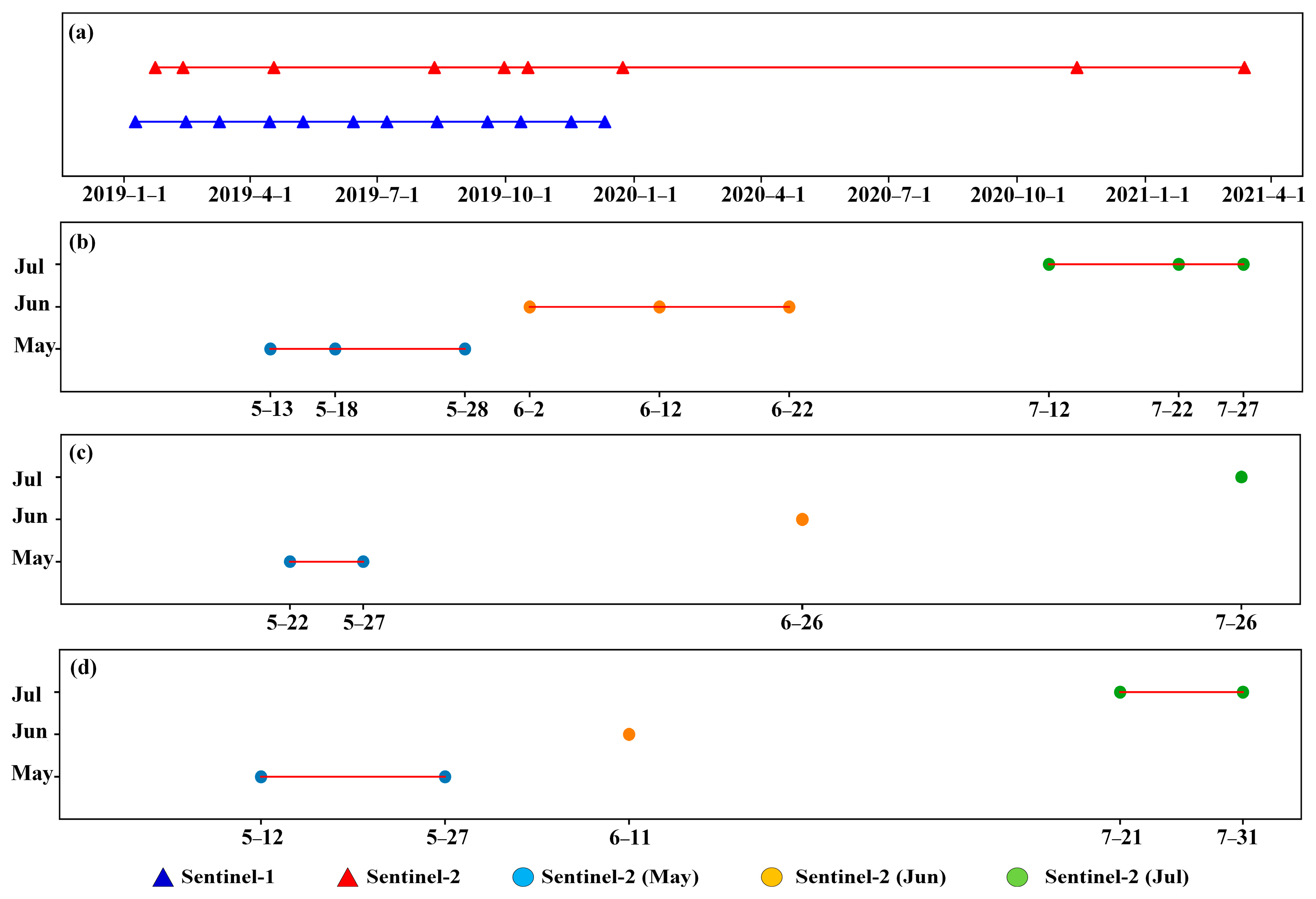
In terms of radar data, C-band (5.3 GHz) polar-orbiting SAR imagery from S1A was collected from the Copernicus Open Access Hub (https://scihub.copernicus.eu/dhus/#/home, accessed on 10 March 2023) for the period of 2019. The S1A mission, launched on 3 April 2014, has created new possibilities for estimating forest AGB by employing backscattering coefficients, owing to its free-access and global-coverage features, frequent revisits, and prompt product supply. The multilook ground range detected (GRD) product type was used to acquire the data with VV and VH polarizations and the mode interferometric wide swath (IW) [48]. Twelve S1 images (one image per month in 2019) were used in this study (Figure 2). Five preprocessing procedures, including orbit file application, thermal noise removal, radiometric calibration, speckle filtering, and terrain correction, were used in the Sentinel Application Platform (SNAP) version 9.0 of the ESA for all images. Precise orbit files were utilized to update and refine the orbit state vectors of the GRD products, which were typically inaccurate. The SNAP model was used to remove thermal noise, thereby improving the quality of the image data by distinguishing random interference from the desired signal. The radiometric calibration converted the SAR image pixel values to backscattering coefficients. The Refined Lee Filter was chosen for its superior performance in alleviating image speckle and enhancing backscatter interpretation compared with other filter algorithms [49]. The 30 m Shuttle Radar Topographic Mission was employed in the Range-Doppler Terrain Correction for terrain correction [50]. Subsequently, all the images were projected to the UTM Zone 49N/WGS-84 projection system and clipped according to the study area.
Regarding optical data, we used S2, which is particularly well-suited for modeling the phonological evolution of vegetation. Among the freely available satellites, S2 offers the broadest range of spectral bands, covering the visible and infrared spectra. Thus, it is rendered to be highly sensitive to critical vegetation properties [51]. However, S2 was affected by cloud cover, thereby greatly reducing its usability. Given the slight changes that existed in the forest AGB of our study area in the same month of recent years, the S2 data obtained from 2019 to 2021 were used to obtain many available images (Figure 2). Nine cloud-free images were captured between January and April and from August to December. The images for the remaining months (May to July) were unavailable because of considerable cloud cover. Therefore, the minimum composition was implemented on each band using all of the relatively high-quality observations acquired in the same month between 2019 and 2021 to fill in the gaps (Figure 2). As a result, the cloud-free composite images for the months of May through July were generated. Cloud-shadow masking was applied before the minimum composition according to the threshold method. For each image, the atmospheric correction was executed with the Sen2Cor plugin (version 2.9) in SNAP software, and the Level-1C product was converted to Level-2A [52]. The Level-2A images were resampled to a resolution of 10 m using the bilinear interpolation, whereas the 1, 9, and 10 bands were abandoned [41]. The image was used as a basis for coregistering with LiDAR, with an accuracy of 0.5 pixels, and was clipped according to the study region.

3. Methods

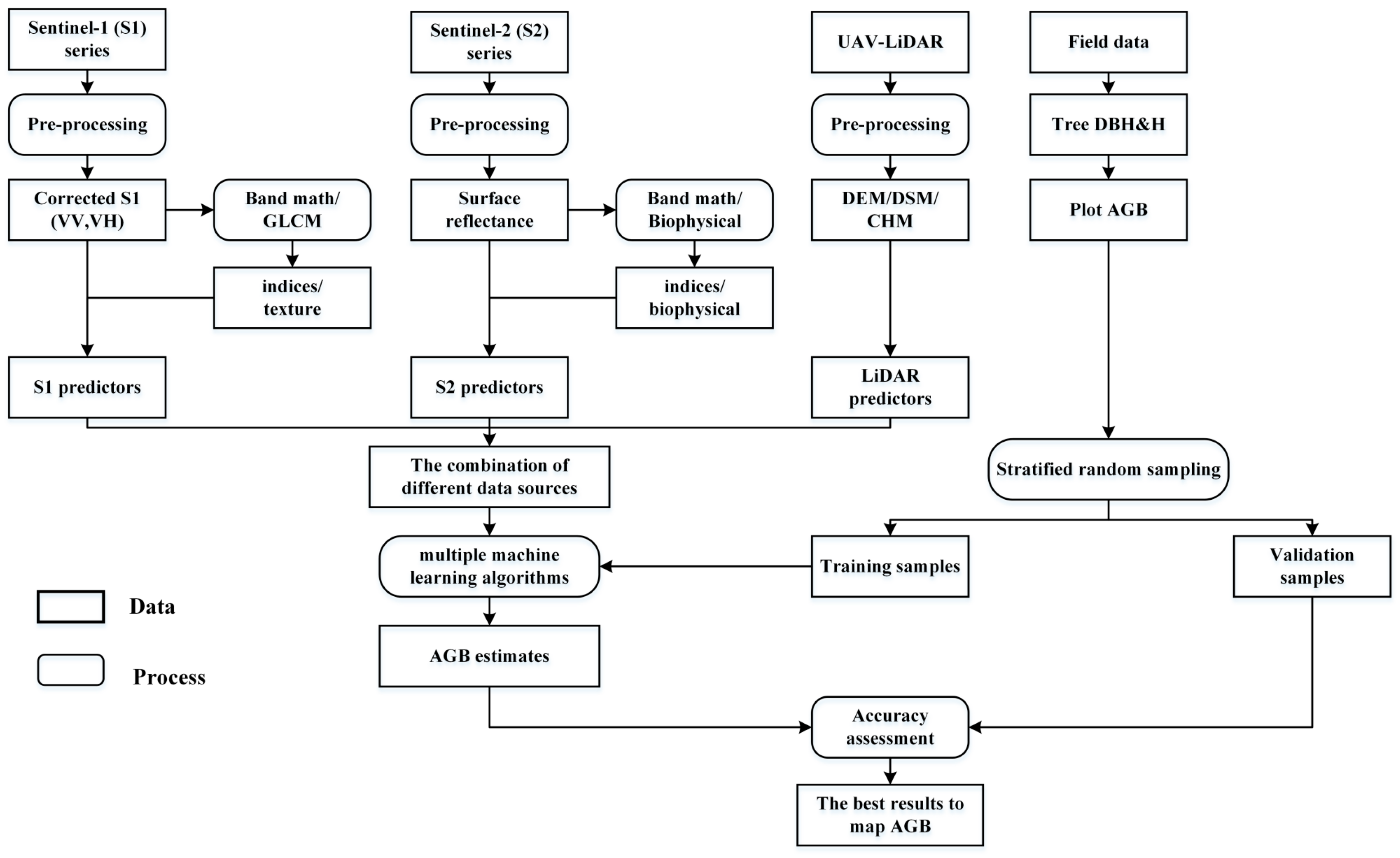
Figure 3 demonstrates the methodological framework for estimating the forest AGB in this study. Seven models were developed using individual and combined backscatter (S1), spectral (S2), and canopy structure (LiDAR) data collected from independent training plots. The established models were evaluated for accuracy using the validation samples. Ultimately, the best-performing model was applied to estimate the wall-to-wall biomass map.

3.1. Predictor Variables

3.1.1. LiDAR Metrics

LiDAR metrics have been proven to be positive predictors of canopy structural parameters (e.g., AGB) [53]. The metrics we derived can be categorized into two groups, namely height metrics and canopy metrics. The height-related metrics portray the geometric structures and distribution of the tree, including percentiles (HpX: X = 10, 20, …, 90), maximum (Hmax), mean (Hmean), variance (Hvar), coefficient of height variation (Hcv), kurtosis (Hkur), and skewness (Hske). The canopy-related metrics describe the canopy density and morphology, including the point densities at different height intervals (PDa_b: a_b = 2_5, 5_10, …, 15_30), canopy cover, and canopy relief ratio [54] (Table 1). These 21 metrics were computed using the first returns, as they were closely associated with the canopy’s surface structure and were stable under different LiDAR acquisition parameter settings (e.g., flying altitude and PD) [55].

3.1.2. Sentinel-1 Metrics

In addition to the polarization bands (VV and VH), the sum (VV + VH), the difference (VV − VH), and the quotient (VV/VH) for each month were calculated based on the published papers [41,44,45] (Table 1). Furthermore, studies based on texture metrics from the SAR data have demonstrated a promising potential to reduce saturation for the parameter estimation of forest structures. The texture metrics derived from small window sizes exhibited a higher sensitivity to fine-scale changes in pixel brightness than those derived from large window sizes [56]. Eight texture metrics were computed based on the VH image with a 3 × 3 window size by using the gray-level co-occurrence matrix, which is a statistical method for measuring the texture characteristics of an image by analyzing the spatial relationships of pixel intensities [57,58] (Table 1).

3.1.3. Sentinel-2 Metrics

Apart from the 10 original bands, three biophysical metrics, i.e., FAPAR, FCOVER, and LAI, were derived through the biophysical processor in SNAP based on the PROSAIL models (Table 1). These metrics are valuable for estimating biomass, as they can reflect the spatial structure of the forest dynamics and state [59,60]. Twelve spectral vegetation metrics, including NDVI, EVI, DVI, RVI, TNDVI, IRECI, MTCI, MCARI, MSRren, STVI1, STVI2, and STVI3, were computed based on their sensitivity to biomass and earlier investigations [41,45,61] (Table 1). All the variables were extracted from the single and composite images.

3.2. Modelling Methods

Seven machine-learning algorithms were compared in the frame of this study (Table 2). They include four major approaches, including (1) tree-based models (SGB, RF, and XGBoost), (2) kernel-based models (GPR), (3) linear models (LASSO), and (4) neural network-based models (CNN and MLP). These models were developed using the Python language, in which CNN was implemented with PyTorch, and other models were achieved with scikit-learn. The best hyperparameters of each model were identified using the grid-search cross-validation method by exploring predefined parameter combinations, as listed in Table 2. A detailed introduction of every algorithm is presented below.
SGB is a boosting ensemble approach that combines the predictions of numerous regression trees. It sequentially fits simple trees using the gradient of the loss function derived by the previous tree to emphasize poorly modeled observations. During each iteration, the input is a randomly selected subset of training data without any substitution [62]. Rather than constructing individual complex trees, small trees are united by taking their weighted averages. The learning process is controlled by tuning four parameters, namely the (Ⅰ) min_samples_split, (Ⅱ) learning_rate, (Ⅲ) max_depth, and (Ⅳ) n_estimators. The SGB algorithm has numerous advantages, including its ability to handle unbalanced training datasets, being slightly affected by outliers, and its robustness in managing predictor interactions [62].
RF is a powerful ensemble learning method that grows a multitude of decision trees, and the final results are provided by calculating the average of predictions of all trees [63]. All trees are produced separately using a bootstrap sample taken from the initial dataset (namely, bagging). Nodes within the trees are split based on a specific number of randomly chosen features (max_features). In our study, max_features was set to “auto”, and RF was computed with n_estimators of 150 and a max_depth of 20, optimized by grid search. RF is robust against data overfitting, outliers, noise, and multicollinearity [64]. Comparative studies including other machine-learning algorithms (e.g., ANN and SVR) showed the superior performance of RF.
XGBoost is an innovative application of the gradient-boosting ensemble technique introduced by [65]. A strong learner is developed by aggregating a set of weak learners by using an additive strategy. The training process begins by fitting a learner using the entire dataset. Subsequently, another learner is incorporated to train on the residual errors generated from the previous learner’s predictions [66]. The training procedure continues to iterate until the specified stopping criterion is met. The final results are derived by aggregating the individual predictions. The main parameters defining the model structure are n_estimators and max_depth, which are turned using grid search. Then, colsample_bytree and subsample are set to 0.8 to prevent overfitting.
GPR has recently been introduced into the domain of estimating biophysical parameters (e.g., LAI) [67]. GPR is a potent regression algorithm that employs a Bayesian probabilistic method to learn regression kernels to fit nonparametric models between features and response variables [68]. The kernel function encodes preexisting assumptions regarding the underlying function (e.g., periodicity and smoothness) by optimizing hyperparameters during the training phase. The radial basis function kernel is applied in this model because of its proven superiority. GPR is further optimized to find a highly suitable combination of length_scale and alpha that maximizes R2. Moreover, length_scale adjusts the shape of the kernel function. Alpha is a regularization parameter. GPR is suitable for handling the anticipated collinearity of the predictors; it also demonstrates superior performance in earlier retrieval studies [69].
LASSO is a statistical regression technique that combines the feature selection and regularization introduced in [70]. The traditional least squares objective function incorporates an L1 penalty term to encourage sparsity in the coefficient estimates. This penalty term, calculated as the sum of the coefficient absolute values multiplied by the parameter alpha, allows for tailored shrinkage in LASSO by adjusting alpha. Lasso automatically performs feature selection by setting some coefficients to zero. Thus, the most important predictors can be identified. Lasso can also handle collinearity among predictors, reduce model complexity, and improve model interpretability.
The CNN used in this study is a basic neural network structure, including three one-dimensional convolutional layers, two max-pooling layers, two batch normalization layers, and one fully connected layer. Kernel sizes of 1 × 3 are set in the convolutional layers to extract predictors from the input data. The nonlinear rectified linear unit is used as the activation function in the three convolutional layers. We used the stochastic gradient descent optimizer to train the CNN by employing mean squared error as the loss function that represents the deviation between the predicted AGB and its truth value. The optimal combination of other parameters, e.g., batch size (412), epochs (203), and learning rate (0.001), were obtained by iteration. The training process involves the adjustment of weights and biases for each neuron using backpropagation to minimize the error [71].
MLP is a fundamental neural network comprising multiple layers of interconnected nodes. It typically includes at least one hidden layer between the input and output layers. Compared with a single-layer perceptron, MLP can grasp complex nonlinear relationships. The training method employs a supervised learning algorithm backpropagation to adjust the network’s internal parameters, including weights and biases. This model is optimized by selecting suitable hidden layers, max_iter, and activation functions. MLP is designed to capture intricate nonlinear predictors from high-dimensional data by using stacked multiple fully connected layers. MLP is a feasible method for estimating AGB [72].

3.3. Modeling Framework and Accuracy Evaluation

This study tested five datasets comprising diverse sets of remote-sensing variables, including (A) S1 features, (B) S2 features, (C) S1 and S2 features, (D) S2 and LiDAR features, and (E) S1, S2, and LiDAR features. Table 3 provides the designs of the experiments. The seven prediction algorithms (SGB, RF, XGBoost, GPR, LASSO, CNN, and MLP) were used for different datasets.
In order to consider the full range of AGB, we divided the AGB measurements into four equally sized groups with intervals of 50 Mg/ha, ranging from 16.32 Mg/ha to 186.50 Mg/ha (Table 4). Within each group, we further divided the AGB samples (n = 804) into training (75%) and validation (25%) datasets (Table 4). For the regression analysis, training and validation datasets were obtained by laying the field sample polygon layer onto an image stack containing all metrics, and the respective values were extracted.
The evaluation of prediction accuracy for each experiment was conducted using the independent 25% testing datasets (N = 201). Three error analysis indices, i.e., coefficient of determination (R2), root mean squared error (RMSE), and relative RMSE (RMSEr), were computed in each experiment (Equations (2)–(4)).
R 2 = 1 i = 1 n   O i E i 2 i = 1 n   O i A i 2
RMSE = n 1 i = 1 n   E i O i 2 1 / 2
RMS E r = n 1 i = 1 n   E i O i 2 1 / 2 n 1 i = 1 n   O i
where O is the observed value, E is the predicted value, and A is the average of the observed values.

4. Results

4.1. Effectiveness of Prediction Models and Data Sources for AGB Estimation

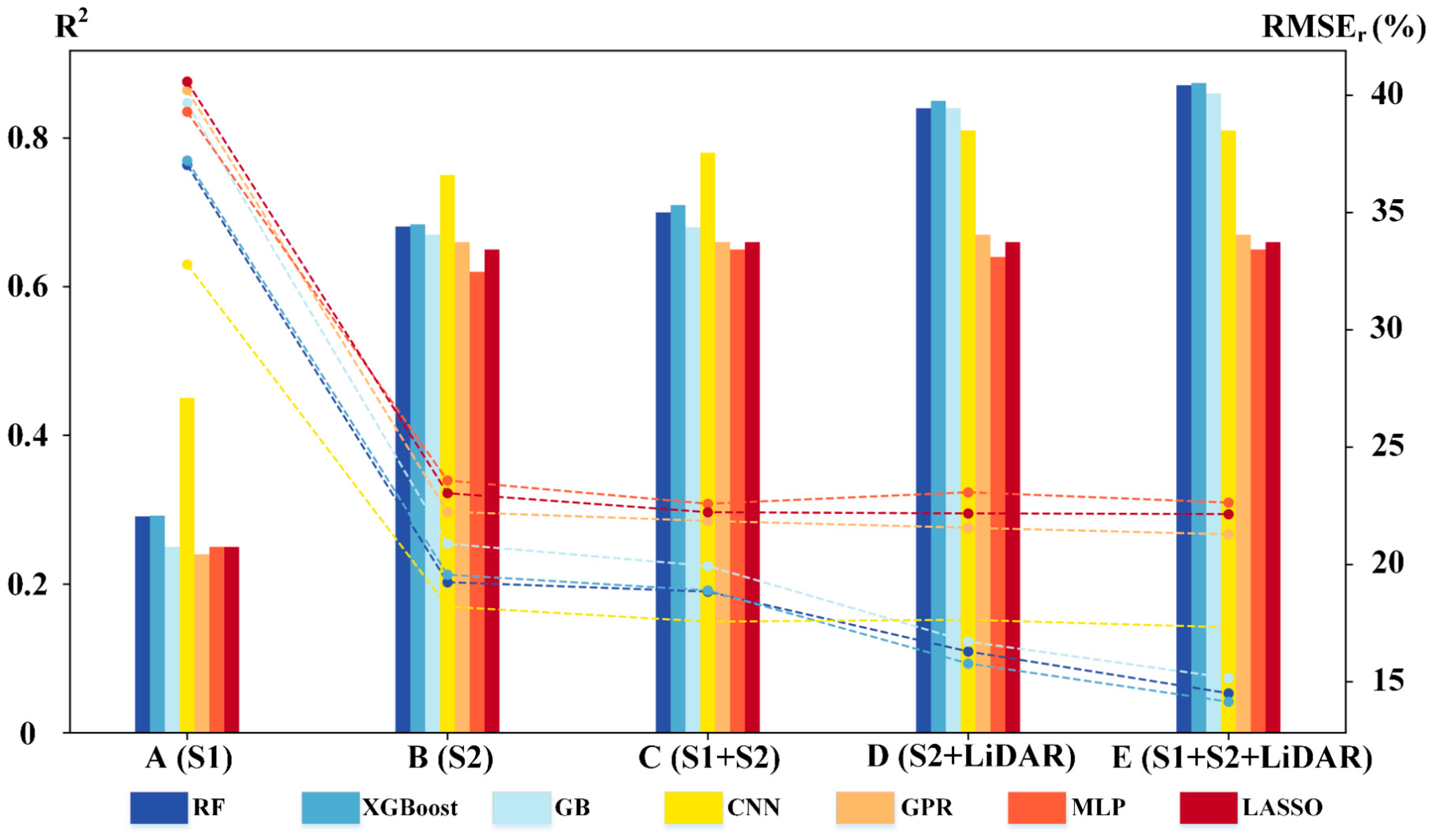
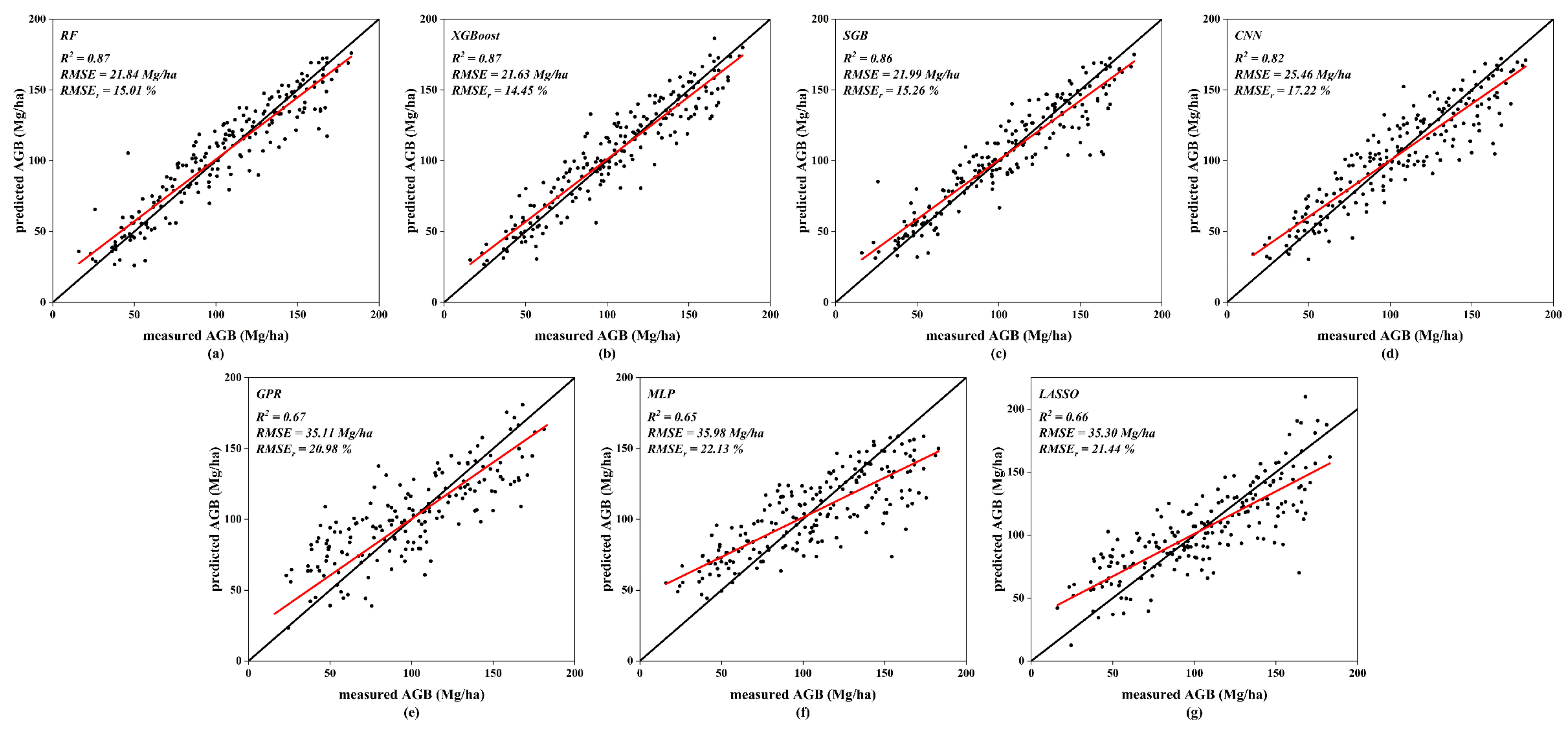
Table 5 and Figure 4 illustrates the validation results from the five experiments performed by combining the S1 and S2 time series and the airborne LiDAR using different prediction algorithms. RF and XGBoost performed similarly across all experiments, with XGBoost demonstrating a slightly higher accuracy than RF. SGB demonstrated consistent performance following RF. All three tree-based models showed favorable performance, with R2 exceeding 0.84 and RMSE reaching below 24 Mg/ha after the incorporation of the LiDAR metrics (experiments D and E). CNN surpassed the other tested models in experiments A–C (S1annual, S2annual, and S1S2annual), with an R2 of 0.45, 0.75, and 0.78 and an RMSE of 47.36, 30.08, and 28.68 Mg/ha, respectively. However, the addition of single-temporal LiDAR metrics in CNN resulted in limited improvement compared to the cases in RF and XGBoost (experiments D and E). The same trend was observed with GPR. GPR exhibited the poorest performance when predicting S1, with an R2 of 0.24 and an RMSE of 56.51 Mg/ha. The poorest performance was afforded by MLP and LASSO, with a low R2 and a high RMSE. The results of experiments A and B illustrate that the annual time series of S2 performed better than those of S1. The use of S2 (experiment B) resulted in improvements in R2 (increase of 0.30–0.42) and RMSE (reduction of 17.28–21.16 Mg/ha) compared to S1 (experiment A) across all prediction models. The best S2annual predicted method and the best S1annual predicted method (prediction model: CNN) differed by 0.3 in R2 and by 17.28 Mg/ha in RMSE. Combining S1 and S2 improved the accuracy of all the prediction models compared to using either data type alone. Specifically, combining S1 and S2 (experiment C) resulted in substantial improvements in R2 (increase of 0.33–0.43) and RMSE (reduction of 18.68–21.37 Mg/ha) relative to using S1 alone (experiment A) across all algorithms. Similarly, compared to using S2 alone (experiment B), the combination of S1 and S2 led to slight improvements in R2 (an increase of 0.01–0.03) and a reduction in RMSE (0.21–2.91 Mg/ha), regardless of the prediction model used. As a result, the XGBoost model with inputs of S1, S2, and LiDAR (experiment E) demonstrated the best performance (R2: 0.87; RMSE: 21.63 Mg/ha; RMSEr: 14.45%). Compared to adding multiple temporal S1 variables, the addition of a single-temporal LiDAR variable to S2 increased the R2 by 0.14 and reduced the RMSE by 10.61 Mg/ha (experiments C and D). Introducing a single-temporal LiDAR variable into S1S1annuanl increased the R2 from 0.71 to 0.87 and reduced the RMSE from 33.35 Mg/ha to 21.63 Mg/ha (experiments C and E). Including S1 in S2Li slightly improved the model accuracy (experiments D and E). Compared with the use of single S2 data (experiment B) for all the algorithms, the addition of LiDAR (experiment D) resulted in improvements in R2 (an increase of 0.01–0.17) and RMSE (a decrease of 0.69–11.41 Mg/ha). Similarly, the addition of LiDAR (experiment D) improved R2 (increase of 0.01–0.18) and RMSE (decrease of 0.11–12.96 Mg/ha) compared to the use of S1S2annual data (experiment C), regardless of prediction models. The scatterplots (Figure 5) of the measured and estimated AGB using the combination of S1, S2, and LiDAR (experiment E) showed that all the models underestimated high AGB while overestimating low AGB values to varying degrees. However, XGBoost was close to the 1:1 line.

4.2. Optimal Variables and Image Acquisition Time to Model AGB

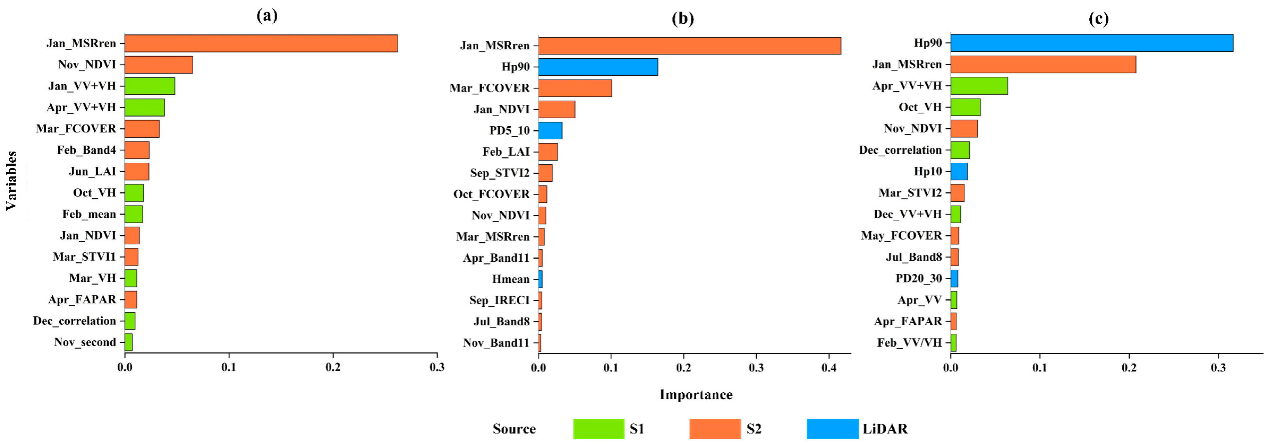
The critical predictors and ideal image acquisition were determined using the sequential forward selection (SFS) method (Figure 6), with the results presented in the variable importance plots shown in Figure 7. With independent-testing datasets, the model performance was assessed by R2. SFS was initiated with an available variable to build a prediction model. Then, it was validated using the testing samples of the corresponding variable. The predictor with the highest R2 was retained. Subsequently, the retained predictor was combined with another variable from the remaining pool (n-1) to form the training data. Then, the model was validated following the same principle. The SFS considered all the potential combinations of variables exhaustively. Moreover, the subset with the highest R2, indicating the subset with the greatest impact on the model, was selected. The variable importance plots present the optimal predictors (top 15) in the combined experiments using the best-performing XGBoost model (experiment C: S1S2annual; experiment D: S2Li; and experiment E: S1S2Li). Compared to spectral bands and SAR backscatter bands, the derivatives were discovered to be preferable predictors of AGB. For experiment C, the most important variable was a red-edge vegetation index (Jan_MSRren), followed by a traditional vegetation index (Nov_NDVI). MSRren was also an important variable in experiments D and E, ranking first and second, respectively. NDVI also held high rankings. The sum of VV and VH (Jan_VV + VH and Apr_VV + VH) was, separately, the third most important variable in experiments C and E involving SAR data. For experiment D, the third important variable was a biophysical measure (Mar_fcover). The plots also indicate that, compared with the VV polarization, the VH polarization was useful for experiments related to SAR, in which VH was ranked as more informative than VV. In addition, the plots show that the sum metrics (VV + VH) were more prominent than the quotient (VV/VH) and difference (VV − VH) metrics in AGB modeling. Among the top 10 most important variables in experiment D, 3 out of 10 were attributed to biophysical variables (Mar_FCOVER, Feb_LAI, and Oct_FCOVER). For experiment C, texture information accounted for 3 out of 15 (Feb_mean, Dec_correlation, and Nov_second). On the whole, optical metrics consistently outnumbered radar metrics (experiments C and E). The most informative LiDAR variable was related to tree height. Among the top three most important variables in the experiment involving LiDAR, Hp90 ranked second and first in experiments D and E, respectively. Additionally, other height-related variables (Hmean and Hp10) were depicted in the plot. Canopy-related PD variables (PD5_10 and PD20_30) were also included. However, the others were not selected by any experiment.
The optimal stages of image acquisition for estimating AGB can be determined in Figure 7. In experiments C and D, the top three most contributing variables were obtained during the dry season from October to March. The majority of the vital variables were derived from the dry season. Among the top 10 most important metrics for experiment C, only two were related to the rainy season (Apr_VV + VH and Jun_LAI). The results of ranking in experiments D and E also show that one (Sep_STVI2) and two (Apr_VV + VH and May_fcover) out of the first ten metrics, respectively, were acquired from the rainy season. Thus, the SAR and optical images in the dry season were discovered to be valuable for forest AGB mapping.

4.3. Spatial Distribution of AGB

Figure 8 depicts the wall-to-wall forest AGB estimations acquired from the XGBoost of the optimal performance by coupling the optical, SAR, and airborne LiDAR metrics. The estimated AGB values ranged from a minimum of 19.63 Mg/ha to a maximum of 189.42 Mg/ha, with an average value of 97.24 Mg/ha. In addition, almost 60% of the AGB values in the study area were between 70 and 140 Mg/ha. The predicted spatial distribution of AGB, including low and high regions, aligns with the actual field measurements. Nevertheless, overestimations or underestimations occurred in sparse or dense forest regions. However, around 60% of the final AGB map fell within the 70 Mg/ha to 140 Mg/ha range, which is consistent with the study area.

5. Discussion

5.1. Difference Data Sources for Modeling AGB

The results of the multisensor remote-sensing metrics, in conjunction with the field data, provided key insights. The S2 data were more suitable for AGB modeling in semiarid forests. This finding was consistent with certain previous investigations that tested the relationship between SAR and optical metrics in AGB mapping [41,73,74]. The poor efficacy of S1 can be ascribed to the limitation of the short wavelength (C-band). When compared with the SAR images with long wavelengths (e.g., P and L bands), the captured C-band SAR images of forests’ vertical structural information have limitations. Recent comparative studies have shown that the textural information derived from S1 makes a great contribution to AGB modeling [75,76], which is in line with our study. This study and [61] showed that VH polarization is more beneficial than VV polarization for AGB modeling. In addition, the SAR metrics sum (VV + VH) had a closer correlation with AGB than VH. Therefore, the integration of the sum metrics and textural information must be considered for AGB modeling. The combination of long-wavelength SAR images (e.g., P and L bands) with S1 and S2 should be considered to compensate for the limitation of S1 and improve AGB modeling accuracy in a further study.
S2 data are insensitive to high biomass in forests beyond canopy closure. However, S2 data still outperformed S1 data. Models based on the S2 time series alone showed reasonably strong fits, thereby affirming the significance of time series to capture seasonal variations in vegetation that characterizes semiarid forests. Comparable findings were documented in other studies that compared SAR and optical data sources of AGB mapping. Ref. [73] conducted a comparative analysis between S2 and ALOS PALSAR2 with the L band for AGB modeling in Iran. Great precision was acquired with S2 spectral metrics (R2: 0.61 for the ALOS PALSAR2 model; R2: 0.83 for the S2 model). In addition to the traditional vegetation indices and spectral bands, the researchers discovered that the inclusion of S2-derived red-edge-based vegetation indices and biophysical parameters was functional for improving the performance of mapping AGB [39,44]. In our research, the biophysical parameters (FCOVER and LAI), along with the vegetation indices (traditional index: NDVI; red-edge-based indices: MSRren and IRECI), optimized the accuracy of biomass prediction. The variable importance plots of experiments further showed the advantage of red-edge and traditional vegetation metrics and biophysical variables for estimating AGB. The improvements in accuracy derived from the integration of time series optical and SAR are consistent with those found in some of the available literature [41,44,77]. The complementarity of S1 and S2 in the imaging approach and data features can account for the predictability of AGB. Optical data can provide canopy-related information, whereas SAR can capture structural information. Moreover, the utilization of the yearly monthly time series of S1 and S2 presents new insights for future AGB mapping in semiarid forests.
The additional use of single-temporal LiDAR variables in experiments D and E significantly improved model performance compared with the cases in experiments B and C, respectively. This finding verified the credibility of AGB predictions based on LiDAR in semiarid forest ecosystems and agreed with the finding in earlier research that used small-footprint airborne LiDAR [78]. Among the diverse sensors, LiDAR is widely acknowledged as a cohesive method of capturing complex canopy structures because of its capability to acquire three-dimensional insights into vegetation. Unlike other studies, our study selected the area with relatively low biomass values, which are insufficient to cause signal saturation. This finding demonstrates that LiDAR is effective in high biomass regions, where it can combine with other sensors to mitigate saturation issues and exhibit low sensitivity to signal saturation. Moreover, it also highlights its potential to improve accuracy significantly in low biomass regions. The comparison of S2Li with S1S2 showed that combining multi-temporal S2 with single-temporal LiDAR significantly enhanced accuracy, surpassing the improvements obtained by integrating multi-temporal S1 (experiments C and D). This finding highlights the substantial information obtained by LiDAR compared with that obtained by S1 in semiarid forests, despite the temporal nature of S1. Moreover, this finding is further confirmed by the minimal increase in accuracy between S1S2LiDAR and S2LiDAR. The LiDAR variables identified as important, as depicted in Figure 7, were comparable with the variables selected in other studies, including the height percentiles [54,79,80], mean height [54,81], and PD attributes [82]. The optimal model was made through the integration of S1, S2, and LiDAR. This model performed particularly well, which is consistent with the findings of other studies [83]. In conclusion, the combined variables, particularly the addition of LiDAR variables, were suitable for semiarid forest AGB retrieval. The widespread utilization of spaceborne LiDAR, such as IceSat-2 and GEDI, also facilitates convenience for large-scale areas. Our study did not include variable selection, a step known to enhance prediction accuracy to some extent. We will integrate this process into our methodology in future studies.

5.2. Performance of Prediction Models

The outstanding function of the XGBoost has been discovered by earlier studies. Ref. [84] used three prediction algorithms to produce a comprehensive map of AGB, with XGBoost yielding the best result among other models (RF and multiple linear regression). Another piece of research carried out by [85] used four models, comprising KNN, RF, SVM, and XGBoost, to estimate biomass, with XGBoost showing the best performance. XGBoost leverages an ensemble of weak prediction models, effectively capturing complicated patterns and dependencies in the data. Moreover, the model uses a gradient-boosting algorithm that optimizes the model by iteratively minimizing loss functions. This algorithm also incorporates regularization techniques to prevent overfitting and handle high-dimensional datasets. In this study, the best model that uses the combined three types of remote-sensing data (S1, S2, and LiDAR) was also created by XGBoost. RF followed closely in terms of performance, and similar results were obtained. The model performed well because of its ensemble of decision trees, random feature selection, and robustness to missing values and outliers. One potential problem in RF is that it relies on using the decision surface with soft linear boundaries, which may not be effective when dealing with limited sample sizes. These tree-based models, including SGB, exhibited comparable performance because they all used the tree structures for decision-making and depended on the same fundamental principle for hierarchical partitioning of the feature space. CNN achieved the highest accuracy in the first three groups of experiments. However, the magnitude of improvement in the last two groups of experiments was smaller than that in tree-based models because of the adequacy of the data structure for the model. One possible reason for the poor performance of the GPR could be the inappropriate selection of the kernel function for the given input data. The different kernel functions of GPR must be evaluated in the future study. The poor accuracy of MLP, particularly for the S2 (experiment B), may be attributed to its sensitivity to noise and outliers in the data. The penalty mechanism used by LASSO could explain the limited improvement in accuracy when it was added to the LiDAR variables.

5.3. Contribution of Predictor in Estimating AGB

With respect to S1, the derivative indices of sum (VV + VH) were the most crucial indices involving S1. However, this finding contradicted the discoveries drawn by [86], who concluded that the seasonal quotient variables hold greater significance in biomass mapping than the sum. Regardless of this discrepancy, both studies emphasized the great contribution of S1 derivatives relative to backscatter bands. Compared with VV, VH exhibited superior predictive performance, making it a robust forecasting factor. Cross-polarization mainly occurs from multiple scattering within the tree canopy. It is less affected by surface conditions than copolarization. The relatively high-ranking correlation, mean, and second in experiment C further confirmed the significance of the S1 texture information, as depicted in the relative variable importance plot. In the case of S2, the red-edge dependent vegetation indices (MSRren and IRECI) and the conventional near-infrared index (NDVI) in this study offered important insights regarding the use of S2 for AGB mapping in semiarid environments. MSRren is the most important optical variable, surpassing the other vegetation indices and biophysical features. The studies of [86] and other scholars showed that the red-edge vegetation index can effectively alleviate the saturation phenomenon in AGB estimation. STVI was present in all variables’ important plots, thereby revealing the advantage of the short-wave infrared (SWIR) vegetation index for monitoring AGB in semiarid forests. Although these variables were originally developed and applied in agricultural applications, this study showed the potential of using these variables to estimate AGB in semiarid systems. The red-edge band is an important indicator band for describing plant pigment status and health conditions, reflecting vegetation growth and biomass changes. It can assess conditions under different environmental pressures. Coupled with the SWIR band, which absorbs water, cellulose, and lignin, the red-edge band is closely correlated with the vegetation nitrogen concentration. Other AGB estimation studies organized in semiarid zones showed that STVI exhibits strong correlations with total ground cover and perennial vegetation [87]. For biophysical parameters, FCOVER provides a greater contribution than LAI and FAPAR. This result, unlike the result in [39], may be attributed to variations in the nature and composition of the modeled vegetation. In reference to LiDAR, Hp90 was the most important variable, indicating that the information related to tree height was highly suitable for AGB mapping in semiarid forests. Therefore, the next important variable was the PD variables across different height intervals. The influence of other LiDAR variables, such as height distribution variability (Hvar, Hcv, Hkur, and Hske), on the inversion of AGB was relatively limited.

5.4. Impact of Seasonality on Data Selection

Regarding the impact of seasonal influences, the variables important plots generated by the XGBoost in the three experiments showed that the data collected during the dry season (October to March) play a major role in AGB mapping in the semiarid forests. In terms of S1, its relatively short wavelength, in contrast to the P and L bands, results in limited canopy penetration, which is suitable for the landscapes in our study area, where branches become exposed as leaves fall from October to March. The responsiveness of the SAR data to seasonal variations is influenced by changes in soil moisture and vegetation water content. These factors decrease the sensitivity of the SAR sensor to AGB, despite the good correlation of the high vegetation cover with the remote-sensing data during the rainy season. Figure 7a,b shows that the S1 variables obtained in the dry season improved the model performance. Our observations regarding seasonality are consistent with those by [44], who used S1 data to predict subtropical forest AGB in Central Guangdong Province, China. They assessed variable importance and found that the most-picked SAR variables were from the dry season and were ranked among the top 10 important variables. The available optical data were challenging to obtain, owing to substantial clouds during the rainy season. In addition, our study used thresholding and minimum synthesis methods to generate cloud-free images for a whole-year time series. Figure 7 shows the superior performance of S2 variables from the dry season in semiarid forests.

6. Conclusions

Semiarid forests are often neglected due to their carbon content and lower biodiversity compared to rainforests, leading to a lack of timely and accurate AGB maps for dry forests. This study developed a transferable and scalable method to map AGB in semiarid forests, emphasizing the considerable potential of combining single-temporal LiDAR-derived variables with yearly multi-temporal S1 and S2 for the reliable mapping of AGB in such forests, since this data captures complementary information of forest heterogeneity and structure that is characterized by dry forests. We designed five experiments, consisting of diverse combinations of features, and used seven prediction models (RF, XGBoost, SGB, CNN, GPR, MLP, and LASSO) to achieve our objectives. We concluded the following.
(1)
Multi-temporal S2 (S2annual) demonstrated superior accuracy compared to S1 (S1annual), and the complementary use of the two types of data (S1S1annual) obtained better prediction performance. The addition of single-temporal LiDAR variables with rich vertical structure information further enhanced the AGB estimation accuracy (S2Li vs S2annual and S1S2Li vs S1S2ananul). Moreover, single-temporal LiDAR variables are more informative than yearly monthly time-series S1, despite the temporal nature of S1 (S1S2annual vs S2Li and S2Li vs S1S2Li);
(2)
Compared with other tested machine-learning algorithms, XGBoost produced the best performance with the optimal combination of data sources (S1, S2, and LiDAR) (R2 = 0.87, RMSE = 21.63 Mg/ha, and RMSEr = 14.45%). The superior performance of the tree-based models demonstrated their robustness, stability, and flexibility;
(3)
The variables sum (VV + VH) in S1 and the texture information based on VH (e.g., correlation and mean) were determined as sensitive to AGB mapping. The most-contributing S2 predictors were considered to be MSRren, NDVI, and FCOVER. Among the LiDAR metrics, the height-related Hp90 was the most important factor. These variables have been proven to be applicable for AGB mapping in semiarid forests;
(4)
Semiarid forests are characterized by distinct dry seasons and climatic variations. The variables obtained during the dry season were more conducive to estimating AGB than those obtained during the rainy season, regardless of whether optical or SAR data were used. This finding made it less necessary for S2 to acquire cloud-free images in the challenging rainy season in dry forests.

Author Contributions

Conceptualization, L.Z. and X.Y.; methodology, L.Z. and X.Y.; formal analysis, Y.W. and J.C.; data curation, Y.W. and J.C.; writing—original draft preparation, X.Y.; writing—review and editing, L.Z., X.Y., Y.W. and J.C.; visualization, X.Y.; project administration, L.Z.; funding acquisition, L.Z. All authors have read and agreed to the published version of the manuscript.

Funding

This work was supported by the National Natural Science Foundation of China under Grant [42171439]; the Qingdao Science and Technology Benefit the People Demonstration and Guidance Program, China, under Grant [22-3-7-cspz-1-nsh]; the Open Research Fund Program of Key Laboratory of Ocean Geomatics, Ministry of Natural Resources, China, under Grant [2021B03].

Data Availability Statement

The final data are available in the [Science Data Bank] at [10.57760/sciencedb.13484]. The processed data used to construct the figures presented in this paper are available upon reasonable request from the corresponding author ([email protected]).

Acknowledgments

We are very grateful for the financial support provided by the above funds. We are also grateful to the European Space Agency for its open data policy. In addition, we express our special gratitude to the editor and anonymous reviewers for their time and efforts in reviewing our work.

Conflicts of Interest

The authors declare no conflicts of interest.

References

  1. Zhao, H.; Li, Z.; Zhou, G.; Qiu, Z.; Wu, Z. Site-Specific Allometric Models for Prediction of Above- and Belowground Biomass of Subtropical Forests in Guangzhou, Southern China. Forests 2019, 10, 862. [Google Scholar] [CrossRef]
  2. Herold, M.; Román-Cuesta, R.M.; Mollicone, D.; Hirata, Y.; Van Laake, P.; Asner, G.P.; Souza, C.; Skutsch, M.; Avitabile, V.; MacDicken, K. Options for monitoring and estimating historical carbon emissions from forest degradation in the context of REDD+. Carbon Balance Manag. 2011, 6, 13. [Google Scholar] [CrossRef]
  3. Lu, D.; Chen, Q.; Wang, G.; Liu, L.; Li, G.; Moran, E. A survey of remote sensing-based aboveground biomass estimation methods in forest ecosystems. Int. J. Digit. Earth 2016, 9, 63–105. [Google Scholar] [CrossRef]
  4. Schröder, J.M.; Ávila Rodríguez, L.P.; Günter, S. Research trends: Tropical dry forests: The neglected research agenda? For. Policy Econ. 2021, 122, 102333. [Google Scholar] [CrossRef]
  5. Mora, F.; Jaramillo, V.J.; Bhaskar, R.; Gavito, M.; Siddique, I.; Byrnes, J.E.K.; Balvanera, P. Carbon Accumulation in Neotropical Dry Secondary Forests: The Roles of Forest Age and Tree Dominance and Diversity. Ecosystems 2018, 21, 536–550. [Google Scholar] [CrossRef]
  6. Akindele, S.O.; LeMay, V.M. Development of tree volume equations for common timber species in the tropical rain forest area of Nigeria. For. Ecol. Manag. 2006, 226, 41–48. [Google Scholar] [CrossRef]
  7. Baldi, G.; Verón, S.R.; Jobbágy, E.G. The imprint of humans on landscape patterns and vegetation functioning in the dry subtropics. Glob. Chang. Biol. 2013, 19, 441–458. [Google Scholar] [CrossRef]
  8. Diodato, L.; Fuster, A. Composition of insect assemblage canopy of subtropical dry forests of Semiarid Chaco, Argentina. Caldasia 2016, 38, 197–210. [Google Scholar] [CrossRef]
  9. Gasparri, N.I.; Parmuchi, M.G.; Bono, J.; Karszenbaum, H.; Montenegro, C.L. Assessing multi-temporal Landsat 7 ETM+ images for estimating above-ground biomass in subtropical dry forests of Argentina. J. Arid Environ. 2010, 74, 1262–1270. [Google Scholar] [CrossRef]
  10. Santos, C.A.G.; do Nascimento, T.V.M.; da Silva, R.M. Analysis of forest cover changes and trends in the Brazilian semiarid region between 2000 and 2018. Environ. Earth Sci. 2020, 79, 418. [Google Scholar] [CrossRef]
  11. Tiessen, H.; Feller, C.; Sampaio, E.V.S.B.; Garin, P. Carbon sequestration and turnover in semiarid savannas and dry forest. Clim. Chang. 1998, 40, 105–117. [Google Scholar] [CrossRef]
  12. He, Z.B.; Yang, J.J.; Du, J.; Zhao, W.Z.; Liu, H.; Chang, X.X. Spatial variability of canopy interception in a spruce forest of the semiarid mountain regions of China. Agric. For. Meteorol. 2014, 188, 58–63. [Google Scholar] [CrossRef]
  13. Cunliffe, A.M.; Brazier, R.E.; Anderson, K. Ultra-fine grain landscape-scale quantification of dryland vegetation structure with drone-acquired structure-from-motion photogrammetry. Remote Sens. Environ. 2016, 183, 129–143. [Google Scholar] [CrossRef]
  14. Mensah, S.; Lokossou, C.J.M.; Assogbadjo, A.E.; Kakaï, R.G. Seasonal variation of environment and conspecific density-dependence effects on early seedling growth of a tropical tree in semi-arid savannahs. Glob. Ecol. Conserv. 2023, 43, e02455. [Google Scholar] [CrossRef]
  15. Rejou-Mechain, M.; Tymen, B.; Blanc, L.; Fauset, S.; Feldpausch, T.R.; Monteagudo, A.; Phillips, O.L.; Richard, H.; Chave, J. Using repeated small-footprint LiDAR acquisitions to infer spatial and temporal variations of a high-biomass Neotropical forest. Remote Sens. Environ. 2015, 169, 93–101. [Google Scholar] [CrossRef]
  16. Du, L.M.; Pang, Y.; Wang, Q.; Huang, C.Q.; Bai, Y.; Chen, D.S.; Lu, W.; Kong, D. A LiDAR biomass index-based approach for tree- and plot-level biomass mapping over forest farms using 3D point clouds. Remote Sens. Environ. 2023, 290, 113543. [Google Scholar] [CrossRef]
  17. Naik, P.; Dalponte, M.; Bruzzone, L. Prediction of Forest Aboveground Biomass Using Multitemporal Multispectral Remote Sensing Data. Remote Sens. 2021, 13, 1282. [Google Scholar] [CrossRef]
  18. Dube, T.; Mutanga, O. Evaluating the utility of the medium-spatial resolution Landsat 8 multispectral sensor in quantifying aboveground biomass in uMgeni catchment, South Africa. ISPRS J. Photogramm. Remote Sens. 2015, 101, 36–46. [Google Scholar] [CrossRef]
  19. Baig, S.; Qazi, W.A.; Akhtar, A.M.; Waqar, M.M.; Ammar, A.; Gilani, H.; Mehmood, S.A. Above Ground Biomass Estimation of Dalbergia sissoo Forest Plantation from Dual-Polarized ALOS-2 PALSAR Data. Can. J. Remote Sens. 2017, 43, 297–308. [Google Scholar] [CrossRef]
  20. Hayashi, M.; Motohka, T.; Sawada, Y. Aboveground Biomass Mapping Using ALOS-2/PALSAR-2 Time-Series Images for Borneo’s Forest. IEEE J. Sel. Top. Appl. Earth Obs. Remote Sens. 2019, 12, 5167–5177. [Google Scholar] [CrossRef]
  21. Dlamini, M.; Chirima, G.; Sibanda, M.; Adam, E.; Dube, T. Characterizing Leaf Nutrients ofWetland Plants and Agricultural Crops with Nonparametric Approach Using Sentinel-2 Imagery Data. Remote Sens. 2021, 13, 4249. [Google Scholar] [CrossRef]
  22. Ahmed, O.S.; Shemrock, A.; Chabot, D.; Dillon, C.; Williams, G.; Wasson, R.; Franklin, S.E. Hierarchical land cover and vegetation classification using multispectral data acquired from an unmanned aerial vehicle. Int. J. Remote Sens. 2017, 38, 2037–2052. [Google Scholar] [CrossRef]
  23. Matikainen, L.; Karila, K.; Hyyppa, J.; Litkey, P.; Puttonen, E.; Ahokas, E. Object-based analysis of multispectral airborne laser scanner data for land cover classification and map updating. ISPRS J. Photogramm. Remote Sens. 2017, 128, 298–313. [Google Scholar] [CrossRef]
  24. Yu, R.Y.; Li, S.S.; Zhang, B.; Zhang, H.Q. A Deep Transfer Learning Method for Estimating Fractional Vegetation Cover of Sentinel-2 Multispectral Images. IEEE Geosci. Remote Sens. Lett. 2022, 19, 6005605. [Google Scholar] [CrossRef]
  25. Zhang, X.; Friedl, M.A.; Schaaf, C.B. Global vegetation phenology from Moderate Resolution Imaging Spectroradiometer (MODIS): Evaluation of global patterns and comparison with in situ measurements. J. Geophys. Res. 2006, 111, 367–375. [Google Scholar] [CrossRef]
  26. Lin, J.; Chen, D.; Wu, W.; Liao, X. Estimating aboveground biomass of urban forest trees with dual-source UAV acquired point clouds. Urban For. Urban Green. 2022, 69, 127521. [Google Scholar] [CrossRef]
  27. Ryan, C.M.; Hill, T.; Woollen, E.; Ghee, C.; Mitchard, E.; Cassells, G.; Grace, J.; Woodhouse, I.H.; Williams, M. Quantifying small-scale deforestation and forest degradation in African woodlands using radar imagery. Glob. Chang. Biol. 2012, 18, 243–257. [Google Scholar] [CrossRef]
  28. Berger, M.; Moreno, J.; Johannessen, J.A.; Levelt, P.F.; Hanssen, R.F. ESA’s sentinel missions in support of Earth system science. Remote Sens. Environ. 2012, 120, 84–90. [Google Scholar] [CrossRef]
  29. Shoko, C.; Mutanga, O. Examining the strength of the newly-launched Sentinel 2 MSI sensor in detecting and discriminating subtle differences between C3 and C4 grass species. ISPRS J. Photogramm. Remote Sens. 2017, 129, 32–40. [Google Scholar] [CrossRef]
  30. Drusch, M.; Del Bello, U.; Carlier, S.; Colin, O.; Fernandez, V.; Gascon, F.; Hoersch, B.; Isola, C.; Laberinti, P.; Martimort, P.; et al. Sentinel-2: ESA’s Optical High-Resolution Mission for GMES Operational Services. Remote Sens. Environ. 2012, 120, 25–36. [Google Scholar] [CrossRef]
  31. Wang, D.; Wan, B.; Qiu, P.; Su, Y.; Guo, Q.; Wang, R.; Sun, F.; Wu, X. Evaluating the Performance of Sentinel-2, Landsat 8 and Pléiades-1 in Mapping Mangrove Extent and Species. Remote Sens. 2018, 10, 1468. [Google Scholar] [CrossRef]
  32. Wulder, M.A.; White, J.C.; Nelson, R.F.; Næsset, E.; Ørka, H.O.; Coops, N.C.; Hilker, T.; Bater, C.W.; Gobakken, T. Lidar sampling for large-area forest characterization: A review. Remote Sens. Environ. 2012, 121, 196–209. [Google Scholar] [CrossRef]
  33. Disney, M. Terrestrial LiDAR: A three-dimensional revolution in how we look at trees. New Phytol. 2019, 222, 1736–1741. [Google Scholar] [CrossRef] [PubMed]
  34. Milenkovic, M.; Schnell, S.; Holmgren, J.; Ressl, C.; Lindberg, E.; Hollaus, M.; Pfeifer, N.; Olsson, H. Influence of footprint size and geolocation error on the precision of forest biomass estimates from space-borne waveform LiDAR. Remote Sens. Environ. 2017, 200, 74–88. [Google Scholar] [CrossRef]
  35. Liu, Y.; Gong, W.; Xing, Y.; Hu, X.; Gong, J. Estimation of the forest stand mean height and aboveground biomass in Northeast China using SAR Sentinel-1B, multispectral Sentinel-2A, and DEM imagery. ISPRS J. Photogramm. Remote Sens. 2019, 151, 277–289. [Google Scholar] [CrossRef]
  36. Wang, D.; Wan, B.; Liu, J.; Su, Y.; Guo, Q.; Qiu, P.; Wu, X. Estimating aboveground biomass of the mangrove forests on northeast Hainan Island in China using an upscaling method from field plots, UAV-LiDAR data and Sentinel-2 imagery. Int. J. Appl. Earth Obs. Geoinf. 2020, 85, 101986. [Google Scholar] [CrossRef]
  37. Feng, Y.Y.; Lu, D.S.; Chen, Q.; Keller, M.; Moran, E.; Dos-Santos, M.N.; Bolfe, E.L.; Batistella, M. Examining effective use of data sources and modeling algorithms for improving biomass estimation in a moist tropical forest of the Brazilian Amazon. Int. J. Digit. Earth 2017, 10, 996–1016. [Google Scholar] [CrossRef]
  38. Tian, X.; Su, Z.B.; Chen, E.X.; Li, Z.Y.; van der Tol, C.; Guo, J.P.; He, Q.S. Estimation of forest above-ground biomass using multi-parameter remote sensing data over a cold and arid area. Int. J. Appl. Earth Obs. Geoinf. 2012, 14, 160–168. [Google Scholar] [CrossRef]
  39. Chen, L.; Ren, C.; Zhang, B.; Wang, Z.; Xi, Y.J.F. Estimation of Forest Above-Ground Biomass by Geographically Weighted Regression and Machine Learning with Sentinel Imagery. Forests 2018, 9, 582. [Google Scholar] [CrossRef]
  40. Chen, L.; Wang, Y.; Ren, C.; Zhang, B.; Wang, Z. Optimal Combination of Predictors and Algorithms for Forest Above-Ground Biomass Mapping from Sentinel and SRTM Data. Remote Sens. 2019, 11, 414. [Google Scholar] [CrossRef]
  41. Forkuor, G.; Benewinde Zoungrana, J.-B.; Dimobe, K.; Ouattara, B.; Vadrevu, K.P.; Tondoh, J.E. Above-ground biomass mapping in West African dryland forest using Sentinel-1 and 2 datasets—A case study. Remote Sens. Environ. 2020, 236, 111496. [Google Scholar] [CrossRef]
  42. Dimobe, K.; Kuyah, S.; Dabré, Z.; Ouédraogo, A.; Thiombiano, A. Diversity-carbon stock relationship across vegetation types in W National park in Burkina Faso. For. Ecol. Manag. 2019, 438, 243–254. [Google Scholar] [CrossRef]
  43. Fang, J.Y.; Liu, G.H.; Xu, S.L. Biomass and net production of forest vegetation in China. Acta Ecol. Sin. 1996, 16, 497–508. [Google Scholar]
  44. Zhang, L.; Zhang, X.; Shao, Z.; Jiang, W.; Gao, H. Integrating Sentinel-1 and 2 with LiDAR data to estimate aboveground biomass of subtropical forests in northeast Guangdong, China. Int. J. Digit. Earth 2023, 16, 158–182. [Google Scholar] [CrossRef]
  45. Shao, Z.F.; Zhang, L.J.; Wang, L. Stacked Sparse Autoencoder Modeling Using the Synergy of Airborne LiDAR and Satellite Optical and SAR Data to Map Forest Above-Ground Biomass. IEEE J. Sel. Top. Appl. Earth Obs. Remote Sens. 2017, 10, 5569–5582. [Google Scholar] [CrossRef]
  46. Zhao, X.; Guo, Q.; Su, Y.; Xue, B. Improved progressive TIN densification filtering algorithm for airborne LiDAR data in forested areas. ISPRS J. Photogramm. Remote Sens. 2016, 117, 79–91. [Google Scholar] [CrossRef]
  47. Hyyppä, J.; Yu, X.; Hyyppä, H.; Vastaranta, M.; Holopainen, M.; Kukko, A.; Kaartinen, H.; Jaakkola, A.; Vaaja, M.; Koskinen, J.; et al. Advances in Forest Inventory Using Airborne Laser Scanning. Remote Sens. 2012, 4, 1190–1207. [Google Scholar] [CrossRef]
  48. Agency, E.S. Sentinel-1 User Handbook; European Space Agency: Paris, France, 2013.
  49. Lukin, V.; Rubel, O.; Kozhemiakin, R.; Abramov, S.; Shelestov, A.; Lavreniuk, M.; Meretsky, M.; Vozel, B.; Chehdi, K.J.R.A.; Sensing, A.i.R. Despeckling of multitemporal sentinel SAR images and its impact on agricultural area classification. Remote Sens. 2018, 11, 13. [Google Scholar] [CrossRef]
  50. Small, D.; Schubert, A. Guide to ASAR Geocoding; ESA-ESRIN Technical Note RSL-ASAR-GC-AD; ESA: Paris, France, 2008; Volume 1, p. 36.
  51. Sentinel-2_Team. Sentinel-2 User Handbook; European Space Agency: Paris, France, 2015.
  52. Louis, F.; Couroussé, T.; Gautron, S. Immunohistochemical Methods for the Study of the Expression of Low-Affinity Monoamine Transporters in the Brain. In Neurotransmitter Transporters: Investigative Methods; Bönisch, H., Sitte, H.H., Eds.; Springer: New York, NY, USA, 2016; pp. 91–108. [Google Scholar] [CrossRef]
  53. Zhang, Z.; Cao, L.; She, G. Estimating Forest Structural Parameters Using Canopy Metrics Derived from Airborne LiDAR Data in Subtropical Forests. Remote Sens. 2017, 9, 940. [Google Scholar] [CrossRef]
  54. de Almeida, C.T.; Galvao, L.S.; Ometto, J.P.H.B.; Jacon, A.D.; de Souza Pereira, F.R.; Sato, L.Y.; Lopes, A.P.; de Alencastro Graça, P.M.L.; de Jesus Silva, C.V.; Ferreira-Ferreira, J.; et al. Combining LiDAR and hyperspectral data for aboveground biomass modeling in the Brazilian Amazon using different regression algorithms. Remote Sens. Environ. 2019, 232, 111323. [Google Scholar] [CrossRef]
  55. Thomas, V.; Treitz, P.; McCaughey, J.H.; Morrison, I. Mapping stand-level forest biophysical variables for a mixedwood boreal forest using lidar: An examination of scanning density. Can. J. For. Res. 2006, 36, 34–47. [Google Scholar] [CrossRef]
  56. Kelsey, K.C.; Neff, J.C. Estimates of Aboveground Biomass from Texture Analysis of Landsat Imagery. Remote Sens. 2014, 6, 6407–6422. [Google Scholar] [CrossRef]
  57. Dube, T.; Mutanga, O. Investigating the robustness of the new Landsat-8 Operational Land Imager derived texture metrics in estimating plantation forest aboveground biomass in resource constrained areas. ISPRS J. Photogramm. Remote Sens. 2015, 108, 12–32. [Google Scholar] [CrossRef]
  58. Haralick, R.M.; Shanmugam, K.; Dinstein, I. Textural Features for Image Classification. IEEE Trans. Syst. Man Cybern. 1973, 6, 610–621. [Google Scholar] [CrossRef]
  59. Ronoud, G.; Fatehi, P.; Darvishsefat, A.A.; Tomppo, E.; Praks, J.; Schaepman, M.E. Multi-Sensor Aboveground Biomass Estimation in the Broadleaved Hyrcanian Forest of Iran. Can. J. Remote Sens. 2021, 47, 818–834. [Google Scholar] [CrossRef]
  60. Dahms, T.; Seissiger, S.; Borg, E.; Vajen, H.; Fichtelmann, B.; Conrad, C. Important Variables of a RapidEye Time Series for Modelling Biophysical Parameters of Winter Wheat. Photogramm. Fernerkund. Geoinf. 2016, 2016, 285–299. [Google Scholar] [CrossRef]
  61. Castillo, J.A.A.; Apan, A.A.; Maraseni, T.N.; Salmo, S.G. Estimation and mapping of above-ground biomass of mangrove forests and their replacement land uses in the Philippines using Sentinel imagery. ISPRS J. Photogramm. Remote Sens. 2017, 134, 70–85. [Google Scholar] [CrossRef]
  62. Friedman, J.H. Stochastic gradient boosting. Comput. Stat. Data Anal. 2002, 38, 367–378. [Google Scholar] [CrossRef]
  63. Breiman, L. Random Forests. Mach. Learn. 2001, 45, 5–32. [Google Scholar] [CrossRef]
  64. Belgiu, M.; Drăguţ, L. Random forest in remote sensing: A review of applications and future directions. ISPRS J. Photogramm. Remote Sens. 2016, 114, 24–31. [Google Scholar] [CrossRef]
  65. Chen, T.; He, T.; Benesty, M. xgboost: Extreme Gradient Boosting. arXiv 2016, arXiv:1603.02754. [Google Scholar]
  66. Chen, T.; Guestrin, C. XGBoost: A Scalable Tree Boosting System. In Proceedings of the Proceedings of the 22nd ACM SIGKDD International Conference on Knowledge Discovery and Data Mining, San Francisco, CA, USA, 13–17 August 2016; pp. 785–794. [Google Scholar] [CrossRef]
  67. Verrelst, J.; Rivera, J.P.; Veroustraete, F.; Munoz-Mari, J.; Clevers, J.; Camps-Valls, G.; Moreno, J. Experimental Sentinel-2 LAI estimation using parametric, non-parametric and physical retrieval methods—A comparison. ISPRS J. Photogramm. Remote Sens. 2015, 108, 260–272. [Google Scholar] [CrossRef]
  68. Sinha, S.K.; Padalia, H.; Dasgupta, A.; Verrelst, J.; Rivera, J.P. Estimation of leaf area index using PROSAIL based LUT inversion, MLRA-GPR and empirical models: Case study of tropical deciduous forest plantation, North India. Int. J. Appl. Earth Obs. Geoinf. 2020, 86, 102027. [Google Scholar] [CrossRef]
  69. Verrelst, J.; Munoz, J.; Alonso, L.; Delegido, J.; Rivera, J.P.; Camps-Valls, G.; Moreno, J. Machine learning regression algorithms for biophysical parameter retrieval: Opportunities for Sentinel-2 and -3. Remote Sens. Environ. 2012, 118, 127–139. [Google Scholar] [CrossRef]
  70. Tibshirani, R. Regression Shrinlcage and Selection via the Lasso. J. R. Stat. Soc. Ser. B Stat. Methodol. 1996, 58, 267–288. [Google Scholar] [CrossRef]
  71. Schmidhuber, J. Deep learning in neural networks: An overview. Neural Netw. 2015, 61, 85–117. [Google Scholar] [CrossRef]
  72. Pham, T.D.; Yoshino, K.; Bui, D.T. Biomass estimation of Sonneratia caseolaris (l.) Engler at a coastal area of Hai Phong city (Vietnam) using ALOS-2 PALSAR imagery and GIS-based multi-layer perceptron neural networks. GISci. Remote Sens. 2017, 54, 329–353. [Google Scholar] [CrossRef]
  73. Vafaei, S.; Soosani, J.; Adeli, K.; Fadaei, H.; Naghavi, H.; Pham, T.D.; Tien Bui, D. Improving Accuracy Estimation of Forest Aboveground Biomass Based on Incorporation of ALOS-2 PALSAR-2 and Sentinel-2A Imagery and Machine Learning: A Case Study of the Hyrcanian Forest Area (Iran). Remote Sens. 2018, 10, 172. [Google Scholar] [CrossRef]
  74. Zhao, P.; Lu, D.; Wang, G.; Liu, L.; Li, D.; Zhu, J.; Yu, S. Forest aboveground biomass estimation in Zhejiang Province using the integration of Landsat TM and ALOS PALSAR data. Int. J. Appl. Earth Obs. Geoinf. 2016, 53, 1–15. [Google Scholar] [CrossRef]
  75. Ploton, P.; Barbier, N.; Couteron, P.; Antin, C.M.; Ayyappan, N.; Balachandran, N.; Barathan, N.; Bastin, J.F.; Chuyong, G.; Dauby, G.; et al. Toward a general tropical forest biomass prediction model from very high resolution optical satellite images. Remote Sens. Environ. 2017, 200, 140–153. [Google Scholar] [CrossRef]
  76. Liang, Y.Y.; Kou, W.L.; Lai, H.Y.; Wang, J.; Wang, Q.H.; Xu, W.H.; Wang, H.; Lu, N. Improved estimation of aboveground biomass in rubber plantations by fusing spectral and textural information from UAV-based RGB imagery. Ecol. Indic. 2022, 142, 109286. [Google Scholar] [CrossRef]
  77. Tamga, D.K.; Latifi, H.; Ullmann, T.; Baumhauer, R.; Bayala, J.; Thiel, M. Estimation of Aboveground Biomass in Agroforestry Systems over Three Climatic Regions in West Africa Using Sentinel-1, Sentinel-2, ALOS, and GEDI Data. Sensors 2023, 23, 349. [Google Scholar] [CrossRef]
  78. Almeida, D.R.A.d.; Broadbent, E.N.; Ferreira, M.P.; Meli, P.; Zambrano, A.M.A.; Gorgens, E.B.; Resende, A.F.; de Almeida, C.T.; do Amaral, C.H.; Corte, A.P.D.; et al. Monitoring restored tropical forest diversity and structure through UAV-borne hyperspectral and lidar fusion. Remote Sens. Environ. 2021, 264, 112582. [Google Scholar] [CrossRef]
  79. Longo, M.; Keller, M.; dos-Santos, M.N.; Leitold, V.; Pinagé, E.R.; Baccini, A.; Saatchi, S.; Nogueira, E.M.; Batistella, M.; Morton, D.C. Aboveground biomass variability across intact and degraded forests in the Brazilian Amazon. Glob. Biogeochem. Cycles 2016, 30, 1639–1660. [Google Scholar] [CrossRef]
  80. Gao, L.H.; Chai, G.Q.; Zhang, X.L. Above-Ground Biomass Estimation of Plantation with Different Tree Species Using Airborne LiDAR and Hyperspectral Data. Remote Sens. 2022, 14, 2568. [Google Scholar] [CrossRef]
  81. Latifi, H.; Fassnacht, F.; Koch, B. Forest structure modeling with combined airborne hyperspectral and LiDAR data. Remote Sens. Environ. 2012, 121, 10–25. [Google Scholar] [CrossRef]
  82. Krofcheck, D.J.; Litvak, M.E.; Lippitt, C.D.; Neuenschwander, A. Woody Biomass Estimation in a Southwestern US Juniper Savanna Using LiDAR-Derived Clumped Tree Segmentation and Existing Allometries. Remote Sens. 2016, 8, 453. [Google Scholar] [CrossRef]
  83. Wang, Y.T.; Jia, X.; Chai, G.Q.; Lei, L.T.; Zhang, X.L. Improved estimation of aboveground biomass of regional coniferous forests integrating UAV-LiDAR strip data, Sentinel-1 and Sentinel-2 imageries. Plant Methods 2023, 19, 65. [Google Scholar] [CrossRef]
  84. Li, C.H.; Zhou, L.Z.; Xu, W.B. Estimating Aboveground Biomass Using Sentinel-2 MSI Data and Ensemble Algorithms for Grassland in the Shengjin Lake Wetland, China. Remote Sens. 2021, 13, 1595. [Google Scholar] [CrossRef]
  85. Uniyal, S.; Purohit, S.; Chaurasia, K.; Amminedu, E.; Rao, S.S. Quantification of carbon sequestration by urban forest using Landsat 8 OLI and machine learning algorithms in Jodhpur, India. Urban For. Urban Green. 2022, 67, 127445. [Google Scholar] [CrossRef]
  86. Laurin, G.V.; Balling, J.; Corona, P.; Mattioli, W.; Papale, D.; Puletti, N.; Rizzo, M.; Truckenbrodt, J.; Urban, M. Above-ground biomass prediction by Sentinel-1 multitemporal data in central Italy with integration of ALOS2 and Sentinel-2 data. J. Appl. Remote Sens. 2018, 12, 016008. [Google Scholar] [CrossRef]
  87. Mundava, C.; Helmholz, P.; Schut, A.G.; Corner, R.; McAtee, B.; Lamb, D. Evaluation of vegetation indices for rangeland biomass estimation in the Kimberley area of Western Australia. American journal of pathology. Am. J. Pathol. 2014, 2, 47–53. [Google Scholar] [CrossRef]
Figure 1. Study area: (a) a geographical position map of Qinghai and Gansu Provinces in China; (b) a geographical position map of the study area at the border between Qinghai and Gansu Provinces; and (c) a true color image of the study area formed by clipping an S2 image acquired on 11 August 2019.
Remotesensing 16 03241 g001
Figure 2. Data-acquisition timeline: (a) time of acquisition for the S1 and S2 single image; (b) time of acquisition for the synthetic cloud-free S2 images from May to Jul 2019; (c) time of acquisition for the synthetic cloud-free S2 images from May to Jul 2020; and (d) time of acquisition for the synthetic cloud-free S2 images from May to Jul 2021.
Remotesensing 16 03241 g002
Figure 3. Flowchart of the study.
Remotesensing 16 03241 g003
Figure 4. Accuracy evaluation for different models and data sources. The bar represents R2, and the line represents RMSEr.
Remotesensing 16 03241 g004
Figure 5. Scatter plots of the measured AGB and predicted AGB from the best performance combination (experiment E-S1S2LiDAR) for different models (a) RF; (b) XGBoost; (c) SGB; (d) CNN; (e) GPR; (f) MLP; (g) LASSO.
Remotesensing 16 03241 g005
Figure 6. Flow chart of the sequential forward selection.
Remotesensing 16 03241 g006
Figure 7. Variable importance plots of the top 15 predictors for the XGBoost model with three combined datasets: (a) experiment C; (b) experiment D; (c) experiment E.
Remotesensing 16 03241 g007
Figure 8. AGB map in the study area from the XGBoost model with the optical, SAR, and LiDAR metrics.
Remotesensing 16 03241 g008
Table 1. List of LiDAR, S1, and S2 variables for AGB estimation.
SensorFeatureAbbreviationDefinition/Formula
UAV-LiDARHeightHpXXth (10, 20, 30, 40, 50, 60, 70, 80, or 90th) percentile of height distribution
HmeanMean height
HmaxMaximum height
HvarVariance of height
HskeSkewness of height distribution
HkurKurtosis of height distribution
HcvCoefficient of height variation
Canopy coverPDa_bThe proportion within a height interval a_b (2_5, 5_10, 10_15, 15_30) to the total number of all first returns
COVCanopy cover
CRRCanopy relief ratio
S1PolarizationVVVertical transmit–vertical channel
VHVertical transmit–horizontal channel
IndicesVH − VVDifference
VH + VVSum
VV/VHQuotient
Textural FeaturesCorrelation i , j = 0 N 1 i M e a n j M e a n P i , j 2 V a r i a n c e
Second moment i , j = 0 N 1 i P i , j 2
Variance i , j = 0 N 1 P i , j 1 μ i
Entropy i , j = 0 N 1 i P i , j ln P i , j
Contrast i , j = 0 N 1 i P i , j i j 2
Dissimilarity i , j = 0 N 1 i P i , j i j
Homogeneity i , j = 0 N 1 i P i , j 1 + ( i j ) 2
Mean i , j = 0 N = 1 i P i , j
S2Spectral BandsBand 2490 nm, Blue,
Band 3560 nm, Green,
Band 4665 nm, Red,
Band 5705 nm, Red edge,
Band 6749 nm, Red edge,
Band 7783 nm, Red edge,
Band 8842 nm, Near Infrared (NIR),
Band 8A865 nm, Near Infrared (NIR),
Band 111610 nm, SWIR-1,
Band 122190 nm, SWIR-2,
Conventional near
infrared indices
RVIB8/B4
DVIB8 − B4
EVI[2.5∗(B8 − B4)]/[B8 + 6∗B4 − 7.5∗B2 + 1]
NDVI(B8 − B4)/(B8 + B4)
Red edge indicesMSRren[(B8a/B5) − 1]/[(B8a/B5) − 1]1/2
MSRren[(B5 − B4) − 0.2 × (B5 − B3)] × (B5/B4)
MTCI(B6 − B5)/(B5 − B4)
IRECI(B7 − B4)/(B5/B6)
TNDVI[(B8 − B4)/(B8 + B4) + 0.5]1/2
Shortwave infrared
indices
STVI1(B11∗B4)/B8
STVI2B8/(B4∗B12)
STVI3B8/(B4∗B11)
Biophysical VariablesFAPARFraction of Absorbed Photosynthetically Active Radiation
FCOVERFraction of Vegetation Cover
LAILeaf Area Index
Table 2. Regression models and considered parameters.
TypeAbbr.ModelParameters
tree-basedSGBStochastic Gradient Boostingmin_samples_split, learning_rate, max_depth, n_estimators
RFRandom Forestn_estimators, max_depth, max_features
XGBoosteXtreme Gradient Boostingn_estimators, max_depth, colsample_bytree, subsample
kernel-basedGPRGaussian Process Regressionlength_scale, alpha
linearLASSOLeast Absolute Shrinkage and Selection Operatormax_iter, alpha
neural network-basedCNNConvolutional Neural Networklearning_rate, num_epochs, batch_size
MLPMultilayer Perceptronhidden_layer_sizes, max_iter, activation function
Table 3. Experimental design.
ExperimentNumber of PredictorsDescription/Objective
A: Annual time series of SAR
(S1annual)
156Annual time-series raw polarization bands and their derivatives including difference, sum, quotient bands, and texture features
B: Annual time series of optical (S2annual)300Annual time-series spectral bands and their derivatives, including biophysical parameters and three types of vegetation indices
C: Annual time-series of SAR and optical (S1S2annual)456All obtained annual time-series SAR and optical predictors
D: Optical and LiDAR (S2Li)321Annual time-series optical and single-temporal LiDAR metrics
E: Optical, SAR, and LiDAR (S1S2Li)477All obtained annual time-series SAR, optical predictors, and single-temporal LiDAR metrics
Table 4. Summary of plots and modeling.
Range (Mg/ha)16.32–5050–100100–150150–186.50
Number of plots112256300136
ModelingNumber of training plots (75%)603
Number of validation plots (25%)201
Table 5. Accuracy evaluation for different data sources and models.
ExperimentModelR2RMSE (Mg/ha)RMSRr (%)
A (S1annual)RF0.2954.4737.53
XGBoost0.2954.4637.52
SGB0.2556.3239.76
CNN0.4547.3632.69
GPR0.2456.5139.92
MLP0.2556.2738.79
LASSO0.2556.4539.88
B (S2annual)RF0.6834.5719.74
XGBoost0.6834.6419.86
SGB0.6735.1620.98
CNN0.7530.0818.10
GPR0.6635.8721.94
MLP0.6238.8323.07
LASSO0.6536.2822.33
C (S1S2annual)RF0.7033.8619.34
XGBoost0.7133.3519.19
SGB0.6834.9520.03
CNN0.7828.6817.46
GPR0.6635.4221.55
MLP0.6535.9222.08
LASSO0.6635.4121.52
D (S2Li)RF0.8423.1616.79
XGBoost0.8522.7416.08
SGB0.8423.9216.81
CNN0.8126.0217.54
GPR0.6735.1821.26
MLP0.6436.6322.57
LASSO0.6635.3321.47
E (S1S2Li)RF0.8721.8415.01
XGBoost0.8721.6314.45
SGB0.8621.9915.26
CNN0.8225.4617.22
GPR0.6735.1120.98
MLP0.6535.9822.13
LASSO0.6635.3021.44
Disclaimer/Publisher’s Note: The statements, opinions and data contained in all publications are solely those of the individual author(s) and contributor(s) and not of MDPI and/or the editor(s). MDPI and/or the editor(s) disclaim responsibility for any injury to people or property resulting from any ideas, methods, instructions or products referred to in the content.