Acquisition of Bathymetry for Inland Shallow and Ultra-Shallow Water Bodies Using PlanetScope Satellite Imagery

Abstract

This study is structured to address the problem of mapping the bottom of shallow and ultra-shallow inland water bodies using high-resolution satellite imagery. These environments, with their diverse distribution of optically relevant components, pose a challenge to traditional mapping methods. The study was conducted on several research issues, each focusing on a specific aspect of the SDB, related to the selection of spectral bands and regression models, regression models creation, evaluation of the influence of the number and spatial distribution of reference soundings, and assessment of the quality of the bathymetric surface, with a focus on microtopography. The study utilized basic empirical techniques, incorporating high-precision reference data acquired via an unmanned surface vessel (USV) integrated with a single-beam echosounder (SBES), and Global Navigation Satellite System (GNSS) receiver measurements. The performed investigation allowed the optimization of a methodology for bathymetry acquisition of such areas by identifying the impact of individual processing components. The first results indicated the usefulness of the proposed approach, which can be confirmed by the values of the obtained RMS errors of elaborated bathymetric surfaces in the range of up to several centimeters in some study cases. The work also points to the problematic nature of this type of study, which can contribute to further research into the application of remote sensing techniques for bathymetry, especially during acquisition in optically complex waters.

1. Introduction

Considering the constantly increasing hydrotechnical investments, the provision of bottom relief information plays a crucial role in the water resource exploitation industry. Acquiring bathymetric data of coastal areas, which are affected by constant anthropogenic influences, is also a strategic element in optimizing risk management and shoreline infrastructure development. Hydroacoustic methods for determining underwater topography, such as using single or multibeam echosounders, provide the most precise results [1]. However, regardless of the type of survey platform—manned survey vessel or autonomous craft—these techniques are time-consuming, especially for difficult-to-reach and large-scale areas [2,3].

Due to its high spatial and temporal resolution, remote sensing has become an extremely important technology supporting a range of water-related analyses, including bathymetric data acquisition. Both active and passive techniques [4] allow for the study of large water bodies, with a particular focus on their shallow water parts, aligning with current trends related to reducing human interference in the environment. Nowadays, developments in this field have led to sufficiently qualitative results that, in certain cases, are accepted by many stakeholders, such as the International Hydrographic Organization (IHO) and the International Maritime Organization (IMO) [5,6].

Earlier publications in the field of remote sensing bathymetry have been mainly based on measurements of marine water bodies [7,8,9,10], usually featured by better optical properties than inland waters. Inland waters such as lakes or rivers are characterized by heterogeneous distribution of organic and inorganic compounds, which, among other things, is highlighted in the publication [11], where the authors undertook research related to the determination of water quality parameters in optically complex waters. In addition to local micro-ecosystem variations, the concentration of optically significant components is also influenced by significant periodic changes [12,13]. For this reason, there are notable difficulties in implementing remote sensing bathymetric studies. The spectral response of a water body is a complicated and complex issue, depending on several indirect factors. Reflectance and transmission of water can be variable depending on water characteristics, the type of sediment in suspension, depth, and the geological structure of the bottom [14,15]. For the study of water parameters, earlier solutions to the problem of the optical complexity of water have been based on methods for grouping reflectance spectrums into distinct optical water types using the k-means algorithm and empirical algorithms for estimating water quality parameters [16]. The present study also considers the optical complexity of inland waters but aims to acquire bathymetry.

For hydrographic purposes, the most widely used remote sensing methods are those based on light detection and ranging (LiDAR) technology [17,18,19,20] and those using multispectral imagery [21,22,23,24,25]. There is also a notable trend toward the fusion of active and passive data with a particular focus on satellite sensors [8,26,27,28]. Two main approaches are cited with passive techniques: statistical- and physics-based [2,4]. Statistical refers to identifying correlations between image data and in situ bathymetry, excluding consideration of the physics of light propagation in water and water column properties. This method is only concerned with the statistical relationship between raster values and measured depths and is generally simple to implicate. On the other hand, the physics-based approaches emphasize light propagation in water and its attenuation due to water components and environmental parameters. These techniques rely on a variety of bio-optical and physical–optical water relationships and can be performed both with and without in situ depths. However, this requires advanced knowledge of the physical and biological processes occurring in the studied reservoir, thus increasing the complexity of the applied algorithms. Regarding the well-known passive techniques, the greatest reliability is provided by empirical and semi-empirical methods, where the process is based on a high-precision reference [23,29,30,31]. In the case of studies of reservoirs with transparent water, the most effective penetration ability is guaranteed by wavelengths between 410 and 550 nm, which is in the blue and green radiation range [31,32]. However, in water areas with a strongly varying, seasonally variable environment, it is impossible to determine universal bands to obtain qualitative results [31,32,33]. The extinction of the water tone, which varies at different water column layers, is also a problematic issue, so wave absorption and scattering do not occur linearly. For this reason, it is difficult to specify whether the reflection in shallow water comes from the bottom or from the suspended matter [32].

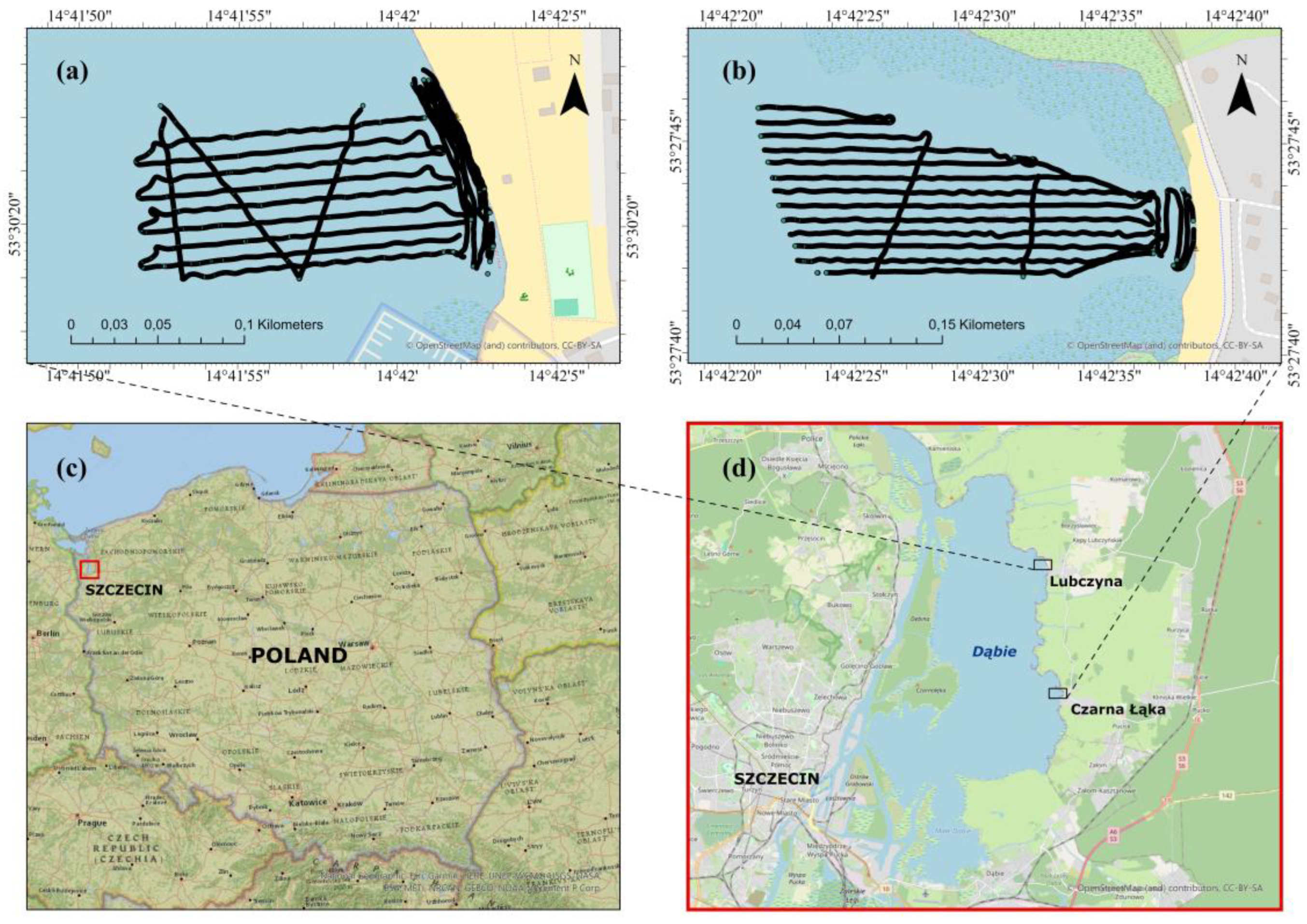
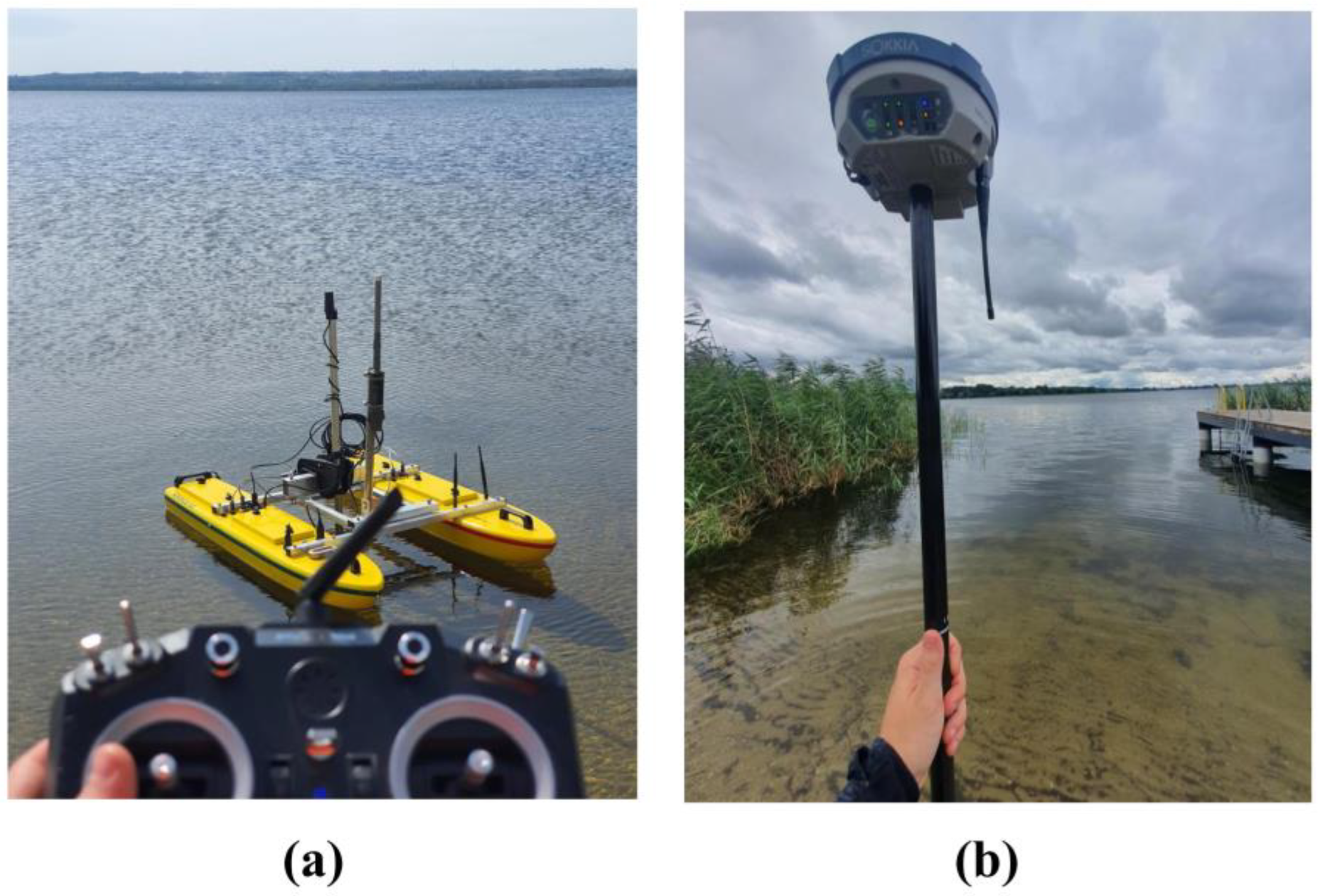
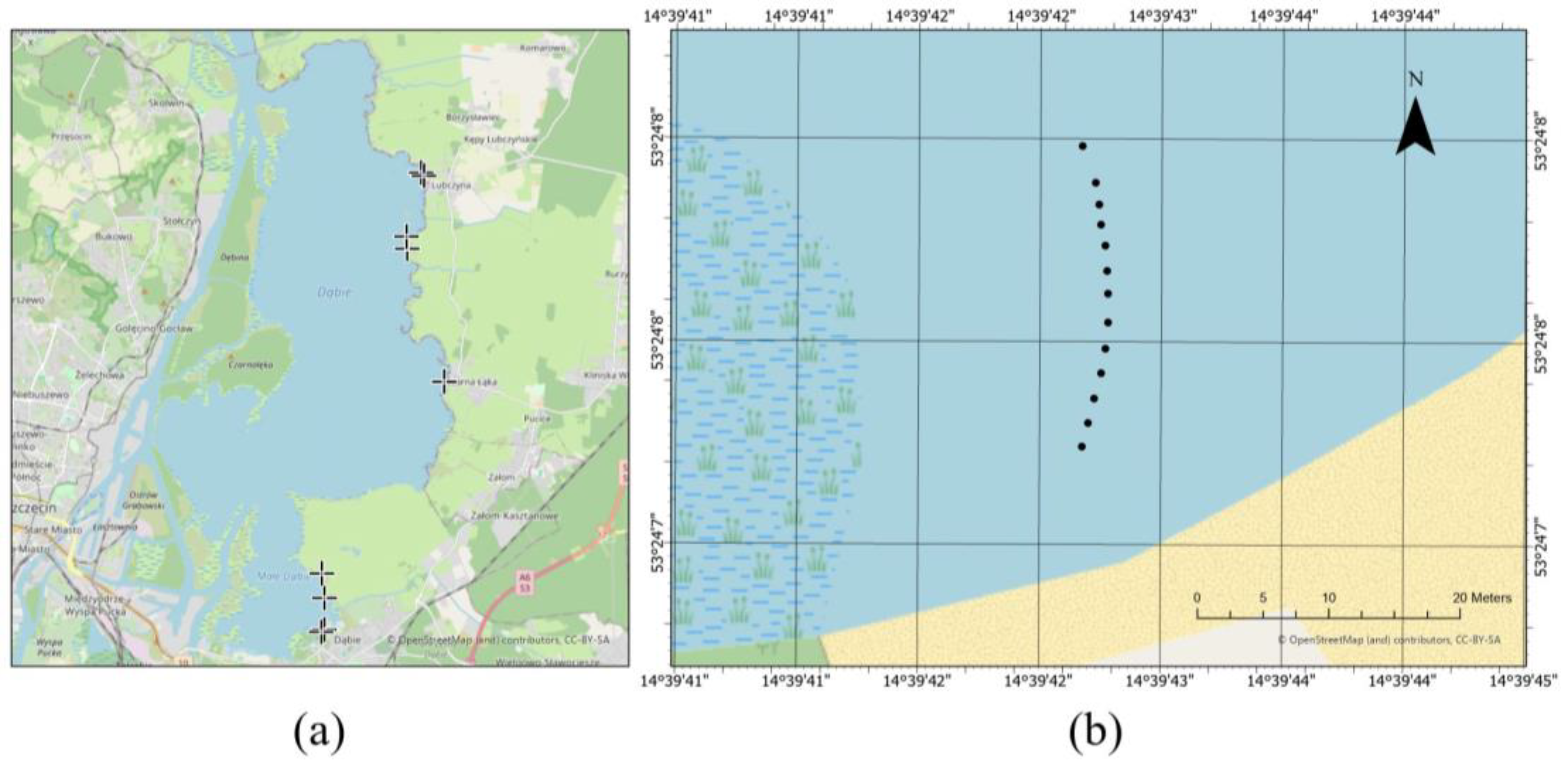
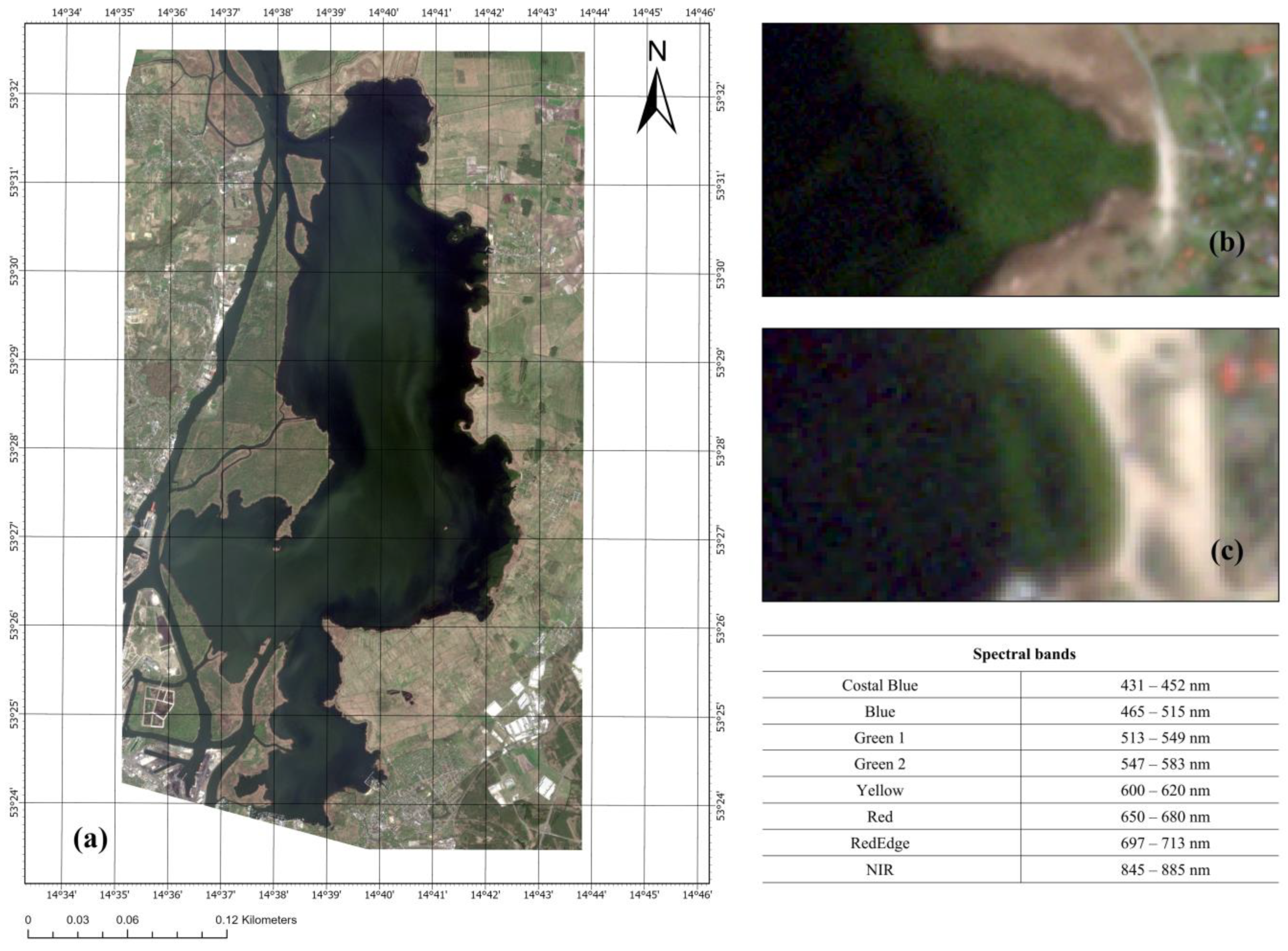
The research in the paper focuses on defining the problem of determining the bathymetry of inland water bodies using high-resolution multispectral satellite imagery. A set of points surveyed using a USV integrated with an SBES and single-measurement profiles based on precise positioning using a GNSS as a bathymetric reference was used. The multispectral imagery was acquired through the PlanetScope mission, which delivers data from eight spectral bands with a three-meter spatial resolution.

The first part of the work focuses on a multivariate analysis of the influence of individual components on the quality of radiometric–bathymetric correlation, where the lake bottom models are created using a regression algorithm [34,35]. The efficiency of the spectral bands and regression models is examined initially. In the next Section, the impact of the distribution and number of reference bathymetric points is studied. In the next step, digital bathymetric models (DBMs) are developed based on different spectral bands and bathymetric reference data. The obtained results were used to verify whether bathymetry sampling strategies have an influence on the accuracy of satellite-derived bathymetry (SDB).

DBMs created by remote sensing techniques are the basis for quantitative and qualitative analysis, which finally leads to a discussion on the effectiveness of individual methods in the context of modeling underwater topography. The entire work also highlights the problem of acquiring bathymetry of inland water bodies, which may imply further future research in this area.

The study’s primary goal was to optimize the methodology for bathymetry acquisition by passive remote sensing methods, with a particular focus on empirical techniques and performing bathymetric surveys for inland shallow and ultra-shallow waters for that aim. Based on comparative analyses, including both quantitative and qualitative assessments, individual input components’ influence on the modeled bottom’s final form was defined. The research also provides essential information on planning and implementing remote sensing bathymetric surveys of water bodies with optically diverse characteristics. The results may find application in the fields of hydrotechnical engineering and biology of aquatic environments, as well as in risk management of coastal areas.

2. Materials and Methods

2.1. Study Area

The study area focuses on the eastern shoreline of Dabie Lake (Jezioro Dąbie in Polish), highlighting two bays located 4.9 km apart (Figure 1). The lake is in the area of Szczecin, in the northwestern part of Poland. The bay near Lubczyna is characterized by an even and gentle increase in depth with increasing distance from the shoreline. However, one exception is an elongated convex dike at about 50 m from the shoreline. The bottom structure is sandy, although it has visible optical differences in distinct parts of the bay. The deepest measured bathymetric point is 2.7 m, while the shallowest is 0.18 m. The total area of the surveyed part of the bay is 2.05 hectares with an average depth oscillating around 1.5 m. The bay near Czarna Laka also features a sandy bottom and a generally evenly deepening profile. The partly irregular shape of the bathymetric surface is caused only by a larger depression visible at the entrance to the bay. The area is dominated by coastal vegetation along the northern and southern borders, giving the bay an elongated shape. The deepest measured bathymetric point is 4.2 m, while the shallowest is 0.24 m. The total area of the surveyed part of the bay is 3.15 hectares with an average depth oscillating around 1.0 m.

2.2. Source Data

Reference bathymetric data were acquired using two different approaches. First, surveys were based on a USV integrated with an SBES. This approach involved the acquisition of bathymetry within two bays of Dabie Lake—near Czarna Laka and Lubczyna—where 7563 and 8042 depth samples were acquired, respectively. To supplement the SBES-based bathymetric surveys, a series of measurement profiles were taken along the eastern shoreline of Dabie Lake using a Sokkia GNSS RTK satellite receiver. The survey equipment is illustrated in Figure 2, and specifications are provided in

Table 1. Basic technical and operational data of the USV.

USV Type: Gerris	GNSS Type: RTK Emlid Reach M2
Length, height, width: 1.2 m, 1 m, 0.36 m	Number of channels: 184
Survey speed: 1.2 m/s	Tracked signals: GPS/QZSS, GLONASS, BeiDou, Galileo
Propulsion: 2 motors T200 Blue Robotics	Frequency of measurement is 20 Hz
Single beam echosounder: Echologger EU400	Accuracy RTK: H: 7 mm + 1 ppm, V: 14 mm + 1 ppm
Echosounder range: 0.15 m~100 m	Data format: NTRIP, RTCM3ERB, text, NMEA (RMC, GGA, GSA, GSV), RINEX2.X, RINEX3.X

and

Table 2. Basic technical data of the GNSS receiver for measuring profile bathymetry points.

GNSS Type: Sokkia GRX1
Number of channels: 72
Tracked signals: GPS, GLONASS, SBAS
Frequency of measurement up to 20 Hz
Accuracy RTK: H 10 mm + 1 ppm, V 20 mm + 1 mm
Data format: RTCM SC104 2.1/2.2/2.3/3.0/3.1, CMR, CMR+, NMEA, TPS

.

Surveys of only the eastern shore resulted from the availability of land accessibility to the reservoir, which was significantly reduced by the undeveloped infrastructural shoreline. Nevertheless, significant impediments to more dense measurements were caused by heavily overgrown reeds on the lake shores. The measurements were performed through a pole-mounted antenna, and the distance between successive points on the profile was about 2 m (Figure 3). The position was determined using the precise Real Time Kinematic (RTK) technique, which allows measurement with centimeter accuracy. Due to the nature of this method, the acquisition of bathymetric samples involved only ultra-shallow areas, where the deepest point measured was 1.06 m, while the shallowest was 0.11 m. The entire point set contained 150 depth samples. The maximum distance between profiles in a straight line was about 12 km, while the minimum was about 120 m. The survey campaign took place on 5th May 2023 (USV) and 28th July 2023 (GNSS), and the weather conditions in both cases were stable, not causing strong water surface agitation.

Satellite imagery acquired through the PlanetScope mission to conduct the study was used. There are three types of remote sensing instruments on board PlanetScope satellites: Dove-Classic, Dove-R, and SuperDove, with the first two acquiring data in only four spectral bands (RGB + NIR) and the third one in eight. The scenes provided by PlanetScope vary in size from about 280 to 630 square kilometers, depending on the type of instrument that captured them. The multispectral sensors mounted aboard each satellite on this mission provide data with three-meter spatial resolution. The products shared by PlanetScope are orthorectified and georeferenced to the Universal Transverse Mercator (UTM) coordinate system [36]. The imagery used in the study is from 21 April 2023 (Figure 4).

2.3. Data Pre-Processing

Pre-processing of input data involves a raster dataset as well as depth samples. The PlanetScope imagery used in the work is a product with the designation “Ortho Analytic 8B SR”. This means that the image has undergone a radiometric correction termed “Surface reflectance”, which is based on top-of-atmosphere (TOA) reflectance and corrects for the effects of the Earth’s atmosphere, accounting for the molecular composition and variation with altitude along with aerosol content [36]. Such a solution is the result of the 6SV model application and MODIS (Moderate-Resolution Imaging Spectroradiometer) data provided by ESA and NASA. The spectral bands used in the study were also subjected to dark object substruction (DOS) correction as a histogram minimum method [37,38] to improve image interpretation potential. This simple method consists of subtracting the darkest pixel value from each spectral band.

Based on the infrared and green bands and the NDWI spectral index (1) [39], a land area mask was created to extract the water area.

$$\mathrm{N}\mathrm{D}\mathrm{W}\mathrm{I}={\displaystyle \frac{({\mathrm{R}}_{\mathrm{G}\mathrm{R}\mathrm{E}\mathrm{E}\mathrm{N}}-{\mathrm{R}}_{\mathrm{N}\mathrm{I}\mathrm{R}})}{({\mathrm{R}}_{\mathrm{G}\mathrm{R}\mathrm{E}\mathrm{E}\mathrm{N}}+{\mathrm{R}}_{\mathrm{N}\mathrm{I}\mathrm{R}})}}$$

(1)

where R_GREEN is the raster value in the green band, and R_NIR is the raster value in the near-infrared band.

Sun-glint correction was not performed in pre-processing because it was difficult to identify within the analyzed areas.

Preparation of reference data, especially in studies devoted to shallow and ultra-shallow water, requires various corrections of input bathymetry. Preprocessing of these data is concerned with both standardizing the vertical reference for bathymetric data and considering the state of the water level. Water level indications were obtained through the Institute of Meteorology and Water Management [40]. A correction was then applied to the hydrographic measurement, and considering the water level on the day and time, PlanetScope captured the image. In addition, the hydroacoustic data were subjected to standard automatic and manual filtering of false echoes caused by, among other things, multiple reflections or suspended matter in the water column. For qualitative comparative analyses, DBMs of the studied bays from bathymetric data acquired by hydroacoustic methods were created (Figure 5).

2.4. Research Methodology

The research process aimed at defining the influence of individual components on the quality of modeled bathymetric surfaces. ArcGIS Pro software (version 3.2.2) was used to perform the data processing tasks. The research was carried out in 4 main stages, focusing on research related to the development of DBMs using satellite imagery and conclusions.

These stages that mainly address DBM development were divided into studies associated with the selection of an appropriate spectral band (stage 1), the selection of a regression model (stage 2), qualitative analysis, and the study of the influence of the spatial distribution of soundings on the final quality of the bathymetric models (stage 3), and the qualitative evaluation of the obtained bathymetric models (stage 4). The quantitative analysis, one of the criteria for evaluating the survey results, was performed and based on the determination of mean, maximum, minimum, and RMSE errors. The specific stages of the study are described below.

• Stage 1

The first stage of the analysis involves determining the spectral band most efficient for a given part of the reservoir. For this purpose, seven spectral bands offered by PlanetScope missions (coastal blue, blue, green 1, green 2, yellow, red, red edge) and an empirical technique were tested based on the procedure proposed by GEBCO [41]. This methodology recommended the blue and green bands from such platforms as Landsat 7 and 8, WorldView 2 and 3, GeoEye-1, and Ikonos-2. In our study, we use only its method of regression model creation. For each regression model creation, we use the basic band instead of the proposed band ratio, i.e., Ln(Blue)/Ln(Green). The reason was the weak efficiency of the blue band in acquiring SDB in our study case. Thus, single bands were tested.

In our case, this method involves determining the averaged raster value (ARV) for unique depth values at 0.1 m intervals. The creation of a model involves only these data. When the pixel values reach a point where, despite a change in depth, their value ceases to change significantly (i.e., bigger depths have nearly the same raster values), it means that the threshold depth (TD), also named as an extinction depth, understood as the maximum depth penetrated by light in this particular case, has been reached at this point. The averaged raster values over depth intervals constitute the final reference data used in subsequent studies. The regression-based model applied in this method is a linear type. A comparison of all observations without and with the GEBCO method is illustrated in Figure 6.

The rationale for this approach was a much better interpretation and overall assessment of the correctness of the regression graph, especially in the areas of ultra-shallow areas. In the classical approach, i.e., using all observations extracted from the image pixels (raster value), a dense dataset is obtained, in which it is difficult to assess to what depth the electromagnetic wave still penetrates the water column, which also means that it can be reflected from the bottom surface. A problem was also noted in the interpretation of the course of the regression function in the area of very shallow depths, which, in these cases, were generally characterized by a very small slope. The selection of the GEBCO approach for further study was preceded by an analysis of all the cases included in the paper. Since it is a method dedicated mainly to marine areas, it was examined in this work in terms of its applicability to inland shallow-water and ultra-shallow-water areas.

The study in this stage included the two water areas by bays discussed in the Introduction and a bathymetric reference based on the USV data. The first evaluation criterion is the R² coefficient from the linear regression and the threshold depth.

• Stage 2

In this stage, a fit analysis of five commonly known regression models (linear, exponential, polynomial, power, and logarithmic) was performed to attempt to define the most effective approach for modeling the bathymetry of shallow-water areas. A comparison with the linear models from Stage 1 was performed.

• Stage 3

The third stage of the analysis focuses on defining the impact of the distribution and number of reference soundings on the quality of bathymetry modeling. This step determines the most efficient band and regression model for each case, following the methodology included in the previous analyses conducted in Stage 1 and 2. Reference data used to build the regression models were bathymetric soundings in different spatial configurations:

• USV surveys from the bay by Lubczyna only;
• USV surveys from the bay by Czarna Laka only;
• USV surveys from both the bay by Czarna Laka and the bay by Lubczyna only;
• GNSS surveys;
• All reference bathymetric points.

Reference soundings provide verification of DBMs elaborated from regression models for each of the five cases for three test options: verification at the Czarna Laka based on the USV survey, verification at Lubczyna based on the USV survey, and verification based on all GNSS profiles. An extensive comparative analysis of the obtained results was performed at this stage.

• Stage 4

This stage involves a study of the accuracy of bottom mapping (qualitative analysis), where digital bathymetric models based on PlanetScope, Sentinel-2, and UAV imaging are compared qualitatively to a reference DBM, elaborated from SBES data. The reconstruction accuracy of individual bays microtopography is treated with special attention.

The research methodology ended with conclusions. It is summarized in Figure 7.

3. Results

Results were compiled according to the stages.

• Stage 1

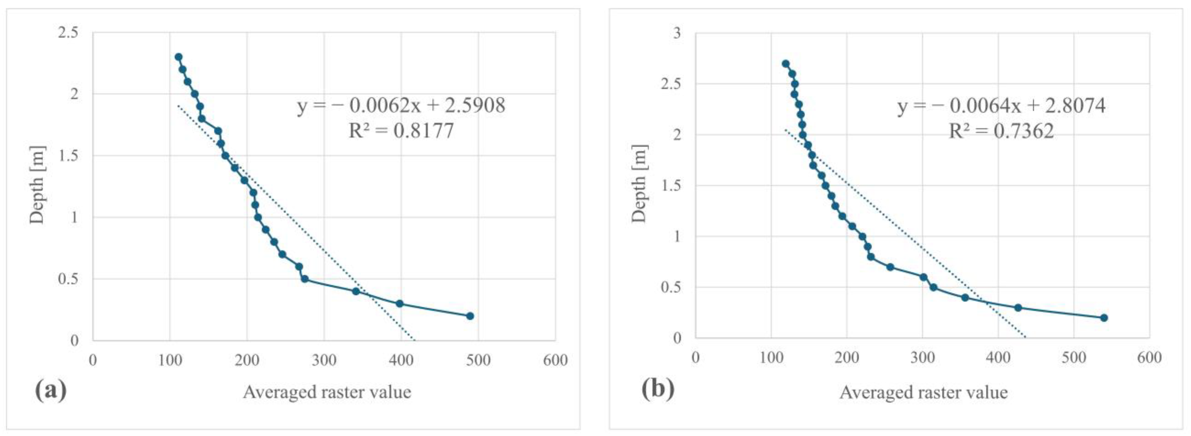
According to stage 1, the level of radiometric–bathymetric correlation was tested on two separate bays using seven spectral bands and an empirical technique. The results of defining the threshold depth according to the GEBCO method show that Lubczyna has a maximum of 2.3 m, while for Czarna Laka it is 2.7 m (

Table 3. Comparison of radiometric–bathymetric correlation results for individual bands, according to GEBCO methodology. R² was calculated based on a linear regression model.

Bay by Lubczyna			Bay by Czarna Laka
Band	Threshold Depth [m]	R2	Band	Threshold Depth [m]	R2
Coastal blue	1.7	0.6558	Costal blue	0.9	0.7885
Blue	2.3	0.7238	Blue	1.0	0.7483
Green	2.3	0.8177	Green	2.3	0.7916
Green 2	2.2	0.7925	Green 2	1.9	0.739
Yellow	2.2	0.7926	Yellow	2.7	0.7362
Red	2.3	0.7196	Red	2.5	0.5859
RedEdge	2.1	0.7469	RedEdge	1.9	0.7516

). For Lubczyna, the green band (513–549 nm) shows the highest R² coefficient from linear regression and the most effective penetration capacity (Figure 8a). For the bay by Czarna Laka, the green band also offers the highest value of the R² coefficient. However, in terms of the range of possible light penetration, much better results are obtained by the yellow band (600–620 nm), which was selected for further analysis (Figure 8b). It potentially enables the acquisition of bathymetry from a deeper part of the water body. As can be seen, with relatively high regression coefficients for the two bands, i.e., for the green band (Lubczyna) R² = 0.8177, and for the yellow band (Czarna Laka) R² = 0.7362, different threshold depth values (TDV) were obtained. From the data acquisition perspective, the band with the higher threshold value should be more effective in acquiring bathymetric data. The analysis of this case already shows the possibility of selecting potentially two bands for the entire reservoir, related to the choice of either the regression model criterion or the criterion of the largest threshold depth value.

• Stage 2

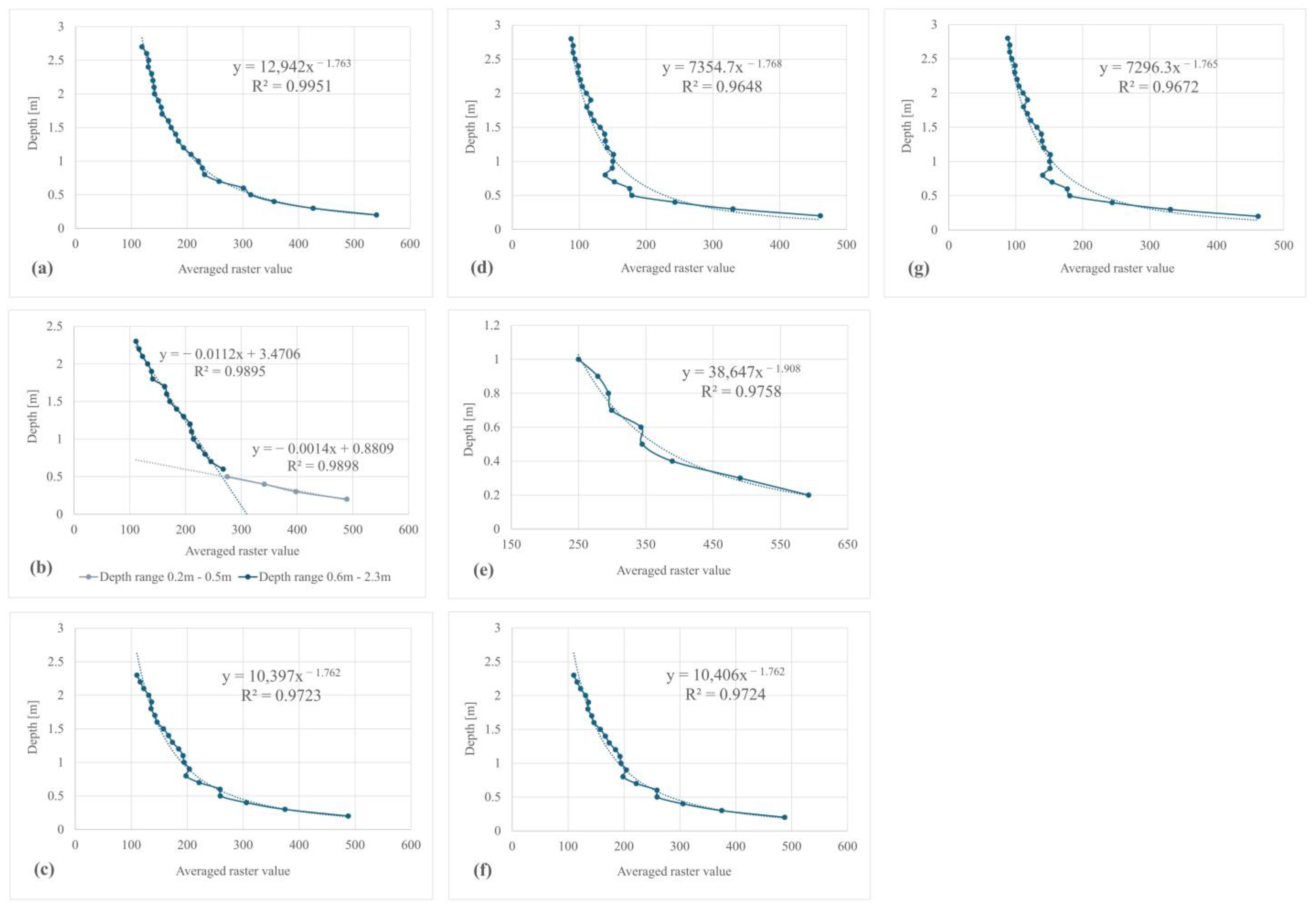
Stage 2 involved analyzing the fit of various regression models based on the spectral bands selected in stage 1—for bay by Lubczyna, the green band, and for bay by Czarna Laka, the yellow band. The results for the nonlinear regressions significantly increased the value of the R² coefficient, showing a lack of linearity in the spectral response of areas from the shallow and ultra-shallow boundaries. Indications for all nonlinear models oscillated around R² = 0.9 (

Table 4. Comparison of radiometric–bathymetric correlation results of selected bands considering different regression models. R² represents models selected based on the best fit to a set of points.

Bay by Lubczyna (Green Band)		Bay by Czarna Laka (Yellow Band)
Regression Type	R2	Regression Type	R2
Linear	0.8177	Linear	0.7362
Polynomial	0.9876	Polynomial	0.9449
Exponential	0.984	Exponential	0.952
Logarithmic	0.9489	Logarithmic	0.8941
Power	0.9373	Power	0.9951

), where the highest observed value for Lubczyna (R² = 0.9876) was guaranteed by a polynomial regression (Figure 9a) and for Czarna Laka (R² = 0.9951) by a power regression (Figure 9c). In the case of the model for the Czarna Laka, a remarkably good fit along the entire depth profile is apparent (Figure 9c). In contrast, the polynomial model for Lubczyna has significant deviations in the ultra-shallow-water depth range (up to 0.5 m). As noted, the regression model in this case (Figure 9a) has a locally weaker fit to the observations. For this reason, despite the relatively high R² coefficient, the fit cannot be described as very good. In addition, the study tried to fit the regression model better. To do so, the area was clustered into two intervals of 0.2 m–0.5 m and 0.6 m–2.3 m, where two independent linear regressions were applied, forming a combined model (Figure 9b). The results of this stage show the possibility of choosing different types of regression functions, including also the creation of combined ones.

• Stage 3

Stage 3 of the study focuses on analyzing the impact of the distribution and quantity of reference surveys on the quality of the resulting modeled bathymetric surface. In this stage, the research is divided into seven experiments, the results of which will allow assessment of the impact of the spatial distribution of reference data acquired in situ. In each option studied, the combination of spectral band and set of reference points is different, thus requiring the creation of new regression models. For this purpose, a new regression model was created for each case analyzed under Stage 3, where the threshold depth was determined according to the GEBCO method, and the nonlinear fit was determined analogously to Stage 2. The characteristics of the reference measurements for each option are included in the study description (Section 2.4). The evaluation criterion will be the quantitative analysis relating to each reference dataset and the differential models between the bathymetric surfaces created using regression models and DBM based on hydroacoustic surveys on the two study bays. The elementary part of the quantitative analysis is the maximum, minimum, mean, and mean squared errors, calculated according to the following Formulas (2)–(5):

$$\mathrm{M}\mathrm{A}\mathrm{X}=\mathrm{m}\mathrm{a}\mathrm{x}\left\{\right(\mathrm{Z}\left(\mathrm{p}\right)-\mathrm{z}\left(\mathrm{p}\right)):\mathrm{p}\in \mathrm{S}\}$$

(2)

$$\mathrm{M}\mathrm{I}\mathrm{N}=\mathrm{m}\mathrm{i}\mathrm{n}\left\{\right(\mathrm{Z}\left(\mathrm{p}\right)-\mathrm{z}\left(\mathrm{p}\right)):\mathrm{p}\in \mathrm{S}\}$$

(3)

where S is a set of reference bathymetric soundings, Z(p) is the depth value at the bathymetric sounding point, and z(p) is the corresponding depth value at the modeled surface.

$$\mathrm{M}\mathrm{E}\mathrm{A}\mathrm{N}={\displaystyle \frac{{\sum }_{\mathrm{i}=1}^{\mathrm{n}}({\mathrm{Z}}_{\mathrm{i}}-{\mathrm{z}}_{\mathrm{i}})}{\mathrm{n}}}$$

(4)

where Z_i is the height measured at a point pi with coordinates (x_i, y_i), z_i is the height of the modeled surface at a point with coordinates (x_i y_i), and n is the number of survey points.

$$\mathrm{R}\mathrm{M}\mathrm{S}\mathrm{E}=\sqrt{{\displaystyle \frac{{\sum }_{\mathrm{i}=1}^{\mathrm{n}}{({\mathrm{Z}}_{\mathrm{i}}-{\mathrm{z}}_{\mathrm{i}})}^2}{\mathrm{n}}}}$$

(5)

The error evaluation was divided into two categories: errors on all surveys of a given type and errors on surveys up to a threshold depth determined by the regression model that is most efficient for a particular experiment. Errors were calculated for seven different experiments as follows:

Experiment 3.1. This experiment tested how a regression model based on the bay by Czarna Laka soundings would affect the construction of DBMs in the Czarna Laka, Lubczyna, and GNSS profile areas.

Experiment 3.2. This experiment tested how a regression model based on the bay by Lubczyna soundings would affect the construction of DBMs in Czarna Laka, Lubczyna, and the GNSS profile area.

Experiment 3.3.1. This experiment was divided into two approaches due to the ambiguity in choosing the most effective spectral band for the case. First, the green band was used. This experiment tested how a regression model based on soundings from both bays by Lubczyna and Czarna Laka would affect the construction of DBMs in Czarna Laka, Lubczyna, and the GNSS profile area.

Experiment 3.3.2. In the next step, it was investigated how a regression model based on the same set of reference soundings and the red band would affect the construction of DBM in Czarna Laka, Lubczyna, and the GNSS profile area.

Experiment 3.4. This experiment tested how a regression model based on GNSS measurements would affect the construction of DBM in Czarna Laka, Lubczyna, and the GNSS profile area.

Experiments 3.5.1 and 3.5.2. These experiments assumed an equivalent methodology to experiment 3, where two spectral bands were tested. The difference is that the regression model can be modified to expand the set of reference soundings with GNSS measurements.

Based on the insights from Stage 1, two different models for the green and red bands were used in experiments 3.3 and 3.5, where the green band guaranteed the best fit (experiment 3.3.1 and experiment 3.5.1), and the red guaranteed the best penetration ability (experiment 3.3.2 and experiment 3.5.2). The key parameters of the regression models selected for use in individual experiments are demonstrated in

Table 5. Summary of the parameters of the regression models used in the various exponents.

	Source of Data	Number of Survey Soundings and ARVs	Band	Regression Type	R2	TDV [m]
Experiment 3.1	USV (Czarna Laka)	7563/26	Yellow	Power	0.9951	2.7
Experiment 3.2	USV (Lubczyna)	8042/22	Green	Combined linear	0.9895, 0.9898	2.3
Experiment 3.3.1	USV (Czarna Laka and Lubczyna)	15,605/22	Green	Power	0.9723	2.3
Experiment 3.3.2	USV (Czarna Laka and Lubczyna)	15,605/27	Red	Power	0.9648	2.8
Experiment 3.4	GNSS Profiles	150/9	Yellow	Power	0.9758	1.0
Experiment 3.5.1	USV and GNSS	15,755/22	Green	Power	0.9724	2.3
Experiment 3.5.2	USV and GNSS	15,605/27	Red	Power	0.9672	2.8

, and graphical representations of the models are shown in Figure 10.

The error values obtained from the DBMs created for each experiment studied are shown in

Table 6. Comparison of calculated errors obtained from specific experiments.

The Source of Reference Points Set Used to Create the Regression Model	Experiment 3.1 (USV, Czarna Laka)				Experiment 3.2 (USV, Lubczyna)				Experiment 3.3.1 (USV, Czarna Laka and Lubczyna)				Experiment 3.3.2 (USV, Czarna Laka and Lubczyna)				Experiment 3.4 GNSS Profiles				Experiment 3.5.1 (USV + GNSS)				Experiment 3.5.2 (USV + GNSS)
	Errors [m]				Errors [m]				Errors [m]				Errors [m]				Errors [m]				Errors [m]				Errors [m]
Validation surveys	MIN	MAX	MEAN	RMSE	MIN	MAX	MEAN	RMSE	MIN	MAX	MEAN	RMSE	MIN	MAX	MEAN	RMSE	MIN	MAX	MEAN	RMSE	MIN	MAX	MEAN	RMSE	MIN	MAX	MEAN	RMSE
Lubczyna Bay	−2.77	1.03	0.10	0.38	−0.53	0.73	0.02	0.16	−2.96	1.00	0.01	0.34	−1.92	1.13	0.13	0.35	−5.62	0.59	−0.43	0.84	−2.96	0.99	0.01	0.34	−1.94	1.12	0.12	0.35
Czarna Laka Bay	−2.27	2.24	−0.02	0.24	−0.97	1.68	−0.19	0.36	−2.77	1.26	−0.11	0.26	−2.39	2.33	−0.25	0.38	−4.91	1.46	−0.30	0.49	−2.78	1.26	−0.11	0.26	−2.41	2.31	−0.26	0.39
GNSS Profiles	−0.47	0.57	0.07	0.18	−0.91	0.48	−0.09	0.30	−0.60	0.54	−0.02	0.20	−0.45	0.69	0.09	0.22	−1.04	0.51	−0.06	0.23	−0.60	0.54	−0.02	0.20	−0.46	0.69	0.09	0.22
	Errors including TD [m]				Errors including TD [m]				Errors including TD [m]				Errors including TD [m]				Errors including TD [m]				Errors including TD [m]				Errors including TD [m]
Validation surveys	MIN	MAX	MEAN	RMSE	MIN	MAX	MEAN	RMSE	MIN	MAX	MEAN	RMSE	MIN	MAX	MEAN	RMSE	MIN	MAX	MEAN	RMSE	MIN	MAX	MEAN	RMSE	MIN	MAX	MEAN	RMSE
Lubczyna Bay	−2.77	1.03	0.10	0.37	−0.53	0.61	0.00	0.14	−2.96	0.76	0.03	0.31	-	-	-	-	−0.91	0.32	0.02	0.09	−2.96	0.76	0.03	0.31	-	-	-	-
Czarna Laka Bay	−2.27	0.83	−0.02	0.18	−0.97	0.30	−0.22	0.33	−2.77	0.64	−0.12	0.25	−1.85	0.90	−0.27	0.37	−1.49	0.15	−0.22	0.29	−2.78	0.64	−0.12	0.24	−1.86	0.89	−0.28	0.37
GNSS Profiles	-	-	-	-	-	-	-	-	-	-	-	-	-	-	-	-	−1.04	0.51	−0.07	0.24	-	-	-	-	-	-	-	-

. The results in the table are divided into two parts—the first concerns the errors of the modeled surfaces including all the soundings in a given case, while the second specifies the errors for observations narrowed to the threshold depth defined by the regression model used in a given experiment. A lack of error values means that the threshold depth of the regression model is greater than the deepest measured bathymetric point in the set of a particular group of validation soundings.

• Analysis of the impact of spatial distribution of bathymetric reference data

At this stage, we will consider four main location cases. The first involves distributing bathymetric reference data in a single location (experiments 3.1 and 3.2, measurement of bathymetry using USV in a single bay). The second concerns the deployment of reference data in two locations (experiments 3.3.3 and 3.3.2, measurement of bathymetry using USV in two bays). The third case involves the use of reference data in a location covering a larger area of a body of water (experiment 3.4, measuring bathymetry with GNSS techniques). The last case also involves the use of reference data in a location covering a larger area of the reservoir, but all reference data are used here (experiments 3.5.1 and 3.5.2, measurement of bathymetry using USV and GNSS).

In the first phase of the error analysis, reference data errors for soundings exceeding the TDV will be evaluated. Based on the results obtained in the first localization case (experiments 3.1 and 3.2), it can be noted that the best results in terms of fitting the modeled surface on the validation points occur when using only local bay reference measurements. This is the case, for instance, when a regression model developed based on surveys from a specific bay is used to create a bottom model. For Lubczyna Bay, expanding the reference set by including soundings taken in the Czarna Laka area and along the eastern line of the lake resulted in an average deviation of the model fit of nearly 20 cm. Analyzing the RMSE error in percentage terms, it can be concluded that using the regression model locally for Czarna Laka reduces its value by 33% (RMSE = 0.24 m), with respect to the case of using the regression model from Lubczyna (RMSE = 0.36 m). The same is true of using the model locally for Lubczyna Bay (RMSE = 0.16 m), where this method of obtaining bathymetry reduces the error by as much as 55%. Clear decreasing trends can also be observed on bias (MEAN errors), while MAX and MIN errors do not always improve. For errors calculated from GNSS measurements, we can conclude that the errors are generally smaller for surfaces based on regression models using only soundings from the bays in question. The RMSE values are 0.18 m and 0.30 m, respectively. The MEAN errors are 0.07 m and −0.09 m, and the MAX and MIN errors range from −0.91 m to 0.57 m.

In the second location case (experiments 3.3.1 and 3.3.2), the impact of regression models created using reference data from two bays was examined. In addition, two types of bands were analyzed: green and red. The green band was selected based on the highest value of R² = 0.9723 (TDV = 2.3 m), while the red band was selected based on the highest value of TVD = 2.8 m (R² = 0.9648). The results indicate an overall performance deterioration with respect to the first localization case. In this variant of the study, we observed an increase in RMSE errors for the bays, with RMS values ranging from 0.26 m to 0.38 m. In three cases, there was a larger deviation in MEAN errors, with values ranging from −0.25 m to 0.13 m. However, in one case, the MEAN error decreased from 0.10 m to 0.01 m. The MIN and MAX errors did not exhibit a clear trend of change but remained within a similar range as in the first localization case, with values ranging from −2.96 m to 2.33 m. Errors calculated on GNSS reference data showed little change. Analyzing the impact of the green and red bands, it can be concluded that using the red band, which has the highest penetration capacity, was less efficient based on the regression model, particularly when modeling the bottom of the bay near Czarna Laka. Compared to the green band, better results using the red band were obtained only in terms of MIN errors.

In the third location case (experiment 3.4), the regression model was verified using only GNSS measurements. The results unequivocally showed that the models developed for the bays performed the worst. The MIN errors ranged from −4.91 m to −5.62 m, the MAX errors from 0.59 m to 1.46 m, the MEAN errors from −0.30 m to −0.43 m, and the RMSE from 0.49 m to 0.84 m. However, the verification using GNSS survey data did not show significant changes compared to the preceding cases.

The final, fourth localization case (experiments 3.5.1 and 3.5.2) verified the regression models built using all reference data, i.e., bathymetric data acquired from USV and GNSS. In addition, two spectral bands—red and green—were analyzed. The results for this localization case were very similar to those obtained in the third localization case. The error values differed by a few centimeters. Hence, they can be interpreted in the same way both in terms of error values and spectral band type.

The results obtained with values up to TDV show an improvement in the results obtained in most cases. For MIN errors, there was a reduction in the error in experiment 3.4 and for red bands in experiments 3.3.2 and 3.5.2 for the bay at Czarna Laka. For the remaining cases, no change was noted. For MAX errors, there was an average change of 51% in their values. MEAN errors were characterized by small changes (ranging from 0.03 to −0.02 m) except for the values obtained in experiment 3.4 (ranging from −0.45 to 0.01 m). Similar changes were observed for the RMSE error, where a decrease was observed ranging from 0.01 to 0.06 m. Larger falls in value up to 0.75 m were noted in experiment 3.4. The results of experiment 3.4 for the threshold depth show that, under certain conditions, it is possible to achieve relatively high precision mapping of areas down to 1 m depth, based on sparsely distributed individual survey profiles. For the bay near Lubczyna, the RMS error value based on this case reached the lowest value among all experiments, guaranteeing model fit with an accuracy of 0.09 m. Similarly, the model on the Czarna Laka, based on an identical regression model and the same threshold depth, presents much worse results, reaching an RMS error value of 0.29 m. The downward trend in the RMS error is illustrated in Figure 11. The summary includes cases of acquiring bathymetry out of and into the TDV depth range.

• Areal analysis of the error distribution

An interesting observation was the tendency of the bathymetric data, in general, to be under or overestimated, and so shift vertically the bathymetric model up or down. In each case, the average MEAN error, which is a measure of surface bias, for the modeled area of the Czarna Laka indicates a tendency to lower the digital bathymetric model. Considering the average error for each experiment, the modeled surface increases depth values by an average of 0.18 m compared to the actual depths. For Lubczyna, the surface statistically is raised in most experiments. The result of this is an average shallowing factor of 0.06 m. The above calculations were performed for all cases with the exclusion of experiment 3.4, where errors were much bigger.

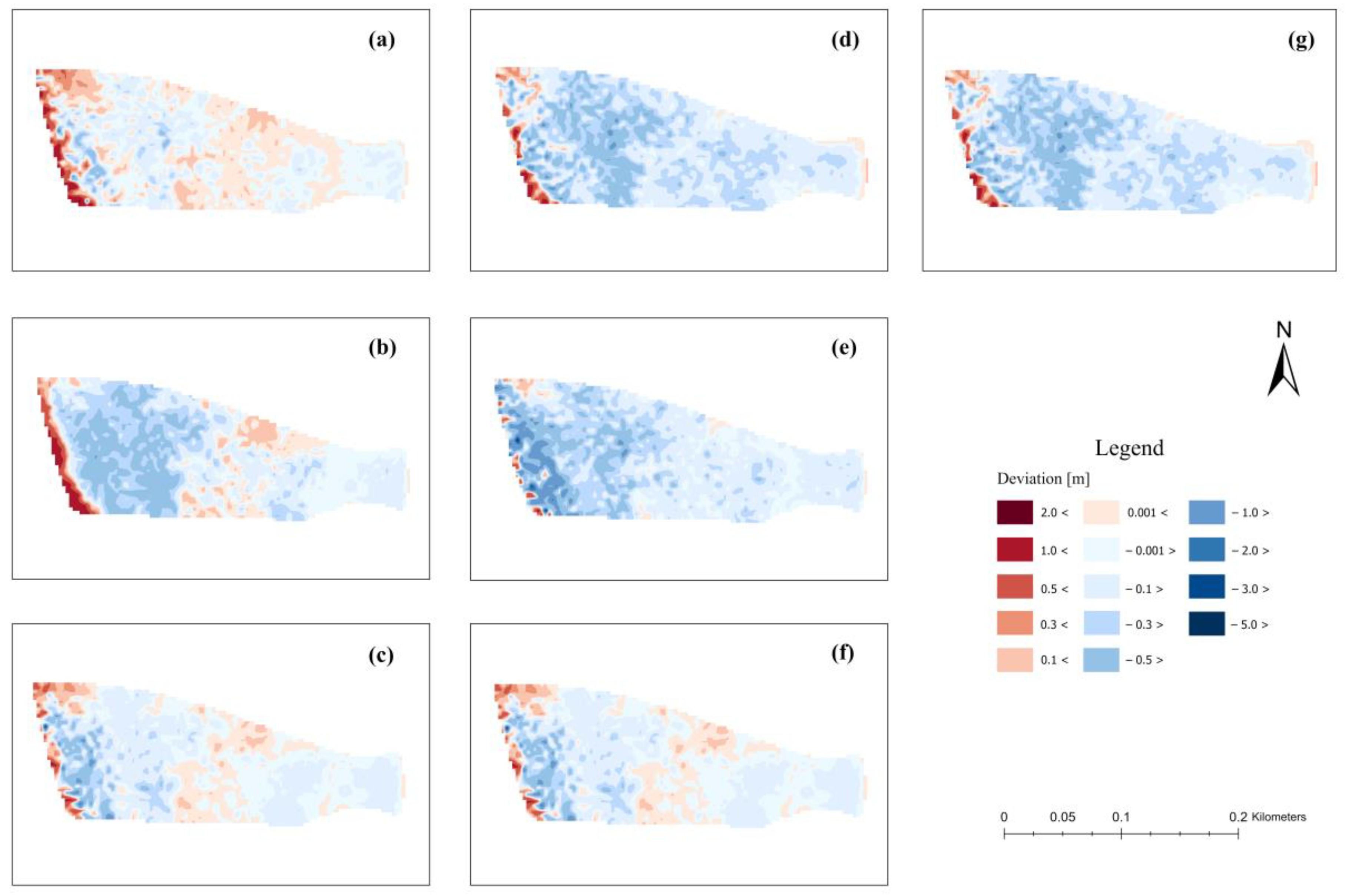
It is also better presented with an areal distribution of deviations from the bathymetric reference surface. For Czarna Laka (Figure 12), areal deviations are mixed, showing a tendency to be lower or upper related to the modeled bathymetric surface. The prevailing tendency is to slightly lower the modeled area relative to the reference bathymetric surface, as visually indicated by the predominance of blue in the graph. 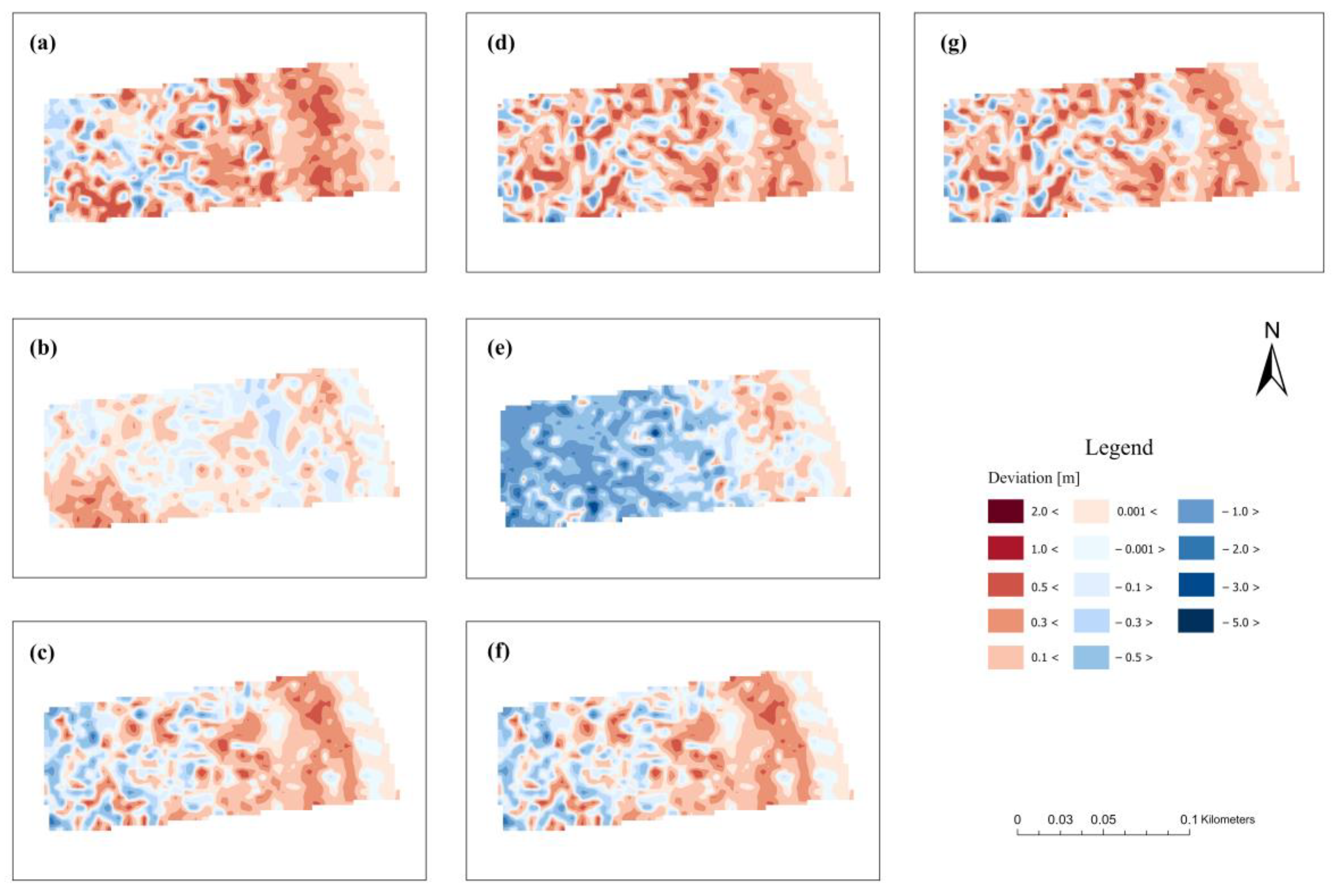This is particularly noticeable in Figure 12b,d,e,g. In the case of Lubczyna, the distribution of errors is strongly heterogeneous (Figure 13). We can visually assess this by the regular interweaving of positive and negative deviations relative to the bathymetric reference surface (visually illustrated by the interweaving of blue and red colors). This rule applies to almost all experimental cases except 3.4 (Figure 13c).

As we can also see, we can observe different trends of deviations in connection with depth for the two cases of bays. In the case of the Czarna Laka, where we have shallower water, we can observe, in most cases, larger values of deviations in the deeper part of the water area. In the adopted color scale, this is visualized by darker shades of red and blue in the left part of the area (Figure 12). On the other hand, we can always observe negative bias in the nearshore area, up to the shoreline. Lubczyna represents the area with deeper water, which may affect the more heterogeneous nature of the deviations (Figure 13). Dominant deviations can be classified as positive, especially in the zone near the shoreline. But in that case, we cannot clearly identify the correlation between increasing depths and deviations due to mix changes, except in the case of experiment 3.4.

Another interesting issue concerns the tendency of modeled surfaces to shallow the dike close to the shoreline of Lubczyna. The result of such a situation is a unique variety of bottom albedo (sandy bottom and local occurrence of bottom sediments) with similar depths in various parts of the bay (Figure 14). Changes in this region can also be observed in Figure 13.

• Analysis of the errors within the depth intervals

However, due to the proportion of values from different depth areas, the threshold depth cannot fully indicate the mapping accuracy capabilities for a given area. In the case of the bay near Czarna Laka, the set of verification points from areas up to 1 m in depth is much larger than the set of points exceeding this value. The result of such a relationship is an artificial underestimation of the fit error for areas characterized by greater depth.

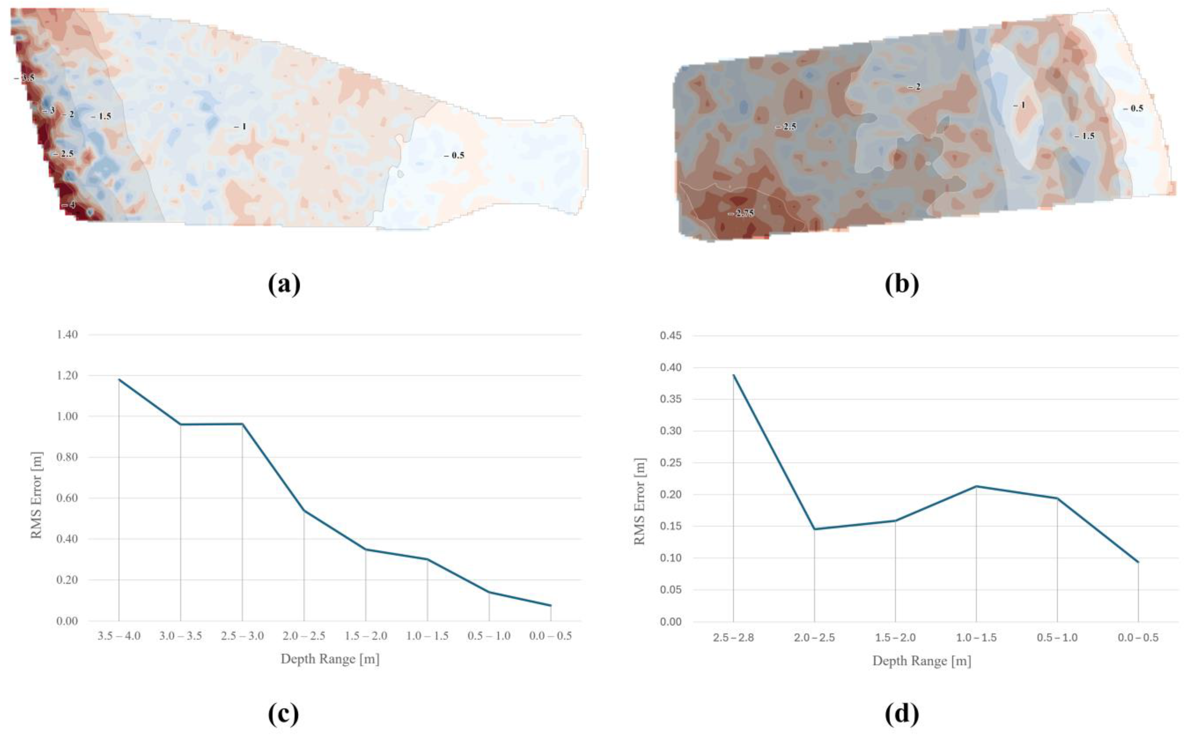
For the two best-modeled surfaces, i.e., those considering measurements only at a given bay, the distribution of RMS error values in each depth interval was examined (Figure 15c,d). In the context of the model created with the best accuracy, the RMS error in the 2.50 m–3.0 m interval increases by as much as more than 0.4 m compared to the 2–2.5 m interval. However, the RMS errors in the given depth intervals for the bay near Czarna Laka indicate that it is possible to map the area to only 1 m depth with very high accuracy, where the RMS does not exceed 0.15 m.

The threshold depth, however, cannot fully indicate the accuracy capabilities of mapping a given area due to the involvement of values from different depth zones. The distribution of errors along the plots modeled for the Lubczyna (Figure 15d) shows a drastic decrease in accuracy only after exceeding 2.5 m depth. In the range from 1.50 m to 2.5 m, the value of the RMS error is lower by several centimeters compared to the 0.50 m–1.5 m range. Therefore, it can be assumed that with an accuracy close to 0.2 m, the Lubczyna area can be mapped to a depth of as much as 2.5 m. The RMS errors in each depth interval for the best model of Lubczyna are much less dependent on depth values than in the case of Czarna Laka (Figure 15a,c).

• Stage 4

Stage 4 of the study is based on a visual assessment of the qualitative mapping capabilities of the bottom characteristics, taking into account microtopography. The area was clipped to a depth limit of 60 cm based on the isobath formed on the reference surface. Since echosounder measurements do not guarantee 100% coverage, the resulting DBM is a spatially interpolated product, where the characteristics of the bottom topography details become difficult to find. Four digital bottom models, resulting from processing data from different sensors, were compared (Figure 16). The surface modeled based on Sentinel-2 satellite imagery reflects the bottom with the worst effect, resulting from the weakest spatial resolution. The nature of the ultra-shallow-water environment requires using sensors with a much smaller pixel size to effectively represent the characteristics of microtopography. In this case, the use of a multispectral camera on an unmanned aerial craft enables the greatest amount of detail to be extracted. The roughness of the bottom surface arises due to the activity of waterfowl in search of food, which leaves characteristic small depressions also visible on the model based on PlanetScope imaging. The DBM based on the PlanetScope provides sufficient information to effectively evaluate the overall trend and bottom features and, in some cases, even microtopography. The SBES data, despite the greatest accuracy in determining individual depth points, lead to an over-generalization of bottom microtopography, resulting in the smooth surface.

4. Discussion

The optical specificity of inland water bodies affects the ambiguity in defining bathymetry from remote sensing imagery. The conducted research was aimed at defining the methodology of acquiring bathymetry from the satellite altitude by assessing the influence of individual processing components on the quality of the created model. However, taking into account the results of the studies received, it turned out to be problematic more than once. The greatest efficiency, in the context of regression model fitting and depth of penetration in general, was achieved by the yellow and green bands (Table 3). Basic assumptions related to the level of light absorption by water show that the best performance should be provided by radiation in the blue range [42]. However, this applies to waters with essentially clear and transparent characteristics. In the cases analyzed, focused on inland water areas, the blue band showed too much limited penetration and, as a result, yielded the worst results. On the other hand, the red band, recommended for measuring waters with a higher turbidity index [31], gave worse readings due to the difficulty of fitting a regression model.

The application of nonlinear models over the linear approach significantly improved the fit of the regression model (Figure 9). In most cases, the power regression model provided the best fit (Table 5, Figure 10). However, in the case of the model based on reference points from the bay near Lubczyna, a linear relationship was used for two depth ranges—one for areas up to about 0.5 m and another for the area in the 0.6–2.3 m range (Figure 9b). For most of the examined options in the third stage, a similar relationship was observed, where the increase in radiometry relative to bathymetry indicated two depth ranges with different optical characteristics (Figure 10). The highest R² coefficient value was observed for the model based on the Czarna Laka reference soundings, where R² = 0.9951. However, such a high correlation coefficient does not directly reflect the precision of the modeled surface. Despite the threshold depth specified by the model as 2.7 m, in the depth range of 1.0–1.5 m, the RMS error was already 0.30 m (Figure 15a,c). Certainly, there is also a noticeable difficulty at this stage in appropriately selecting the type of regression model and interpreting R², at least because of the potential problems associated with mismatching or over-fitting. Another issue is the methodology of building a regression model. Generally, it can be used for all raster values or processed to generalize spectral-depth relations, as was presented in the GEBCO approach [41].

Therefore, it is puzzling which parameters to follow when selecting a spectral band. From the perspective of bottom mapping, the model that guarantees the greatest threshold depth will be the most valuable. On the other hand, the quality of the model can be indicated by the R² coefficient and the overall fit of the model to the data without significant deviations. It was noted in the paper that RMS errors not only increase uniformly with increasing depth but, in some cases, can tend to increase concerning shallower water —as in the case of the local upwelling in the form of a dike (Figure 15b,d). It is generally believed that with increasing depth, measurement accuracy decreases [31]. The analyzed case does not confirm this rule. Similar correlations can be seen in the work of [29] in terms of total vertical uncertainty, in which larger sea areas were surveyed using satellite images of 10 and 30 m resolution. The parameters determined by the regression model cannot definitively guarantee the potential quality of the modeled surfaces. The complexity of radiometric–bathymetric correlations in the case of inland water bodies turns out to be too complicated for the regression model parameters to fully determine the bottom mapping capabilities.

Such complications arise, among other things, from the different bottom albedo, along the same depth values or due to the heterogeneous distribution of bottom sediment. Undoubtedly, this underscores further research into the challenges posed by shallow water and ultra-shallow water for the entire inland waterbody, such as a lake, characterized by great detail of imaged objects. This includes consideration of the possibility of using other geoinformatics techniques or their combination, such as filtering, data clustering, or machine learning methods. It can also include building more complex hybrid models and their further processing. Such a possibility was initially presented in [43,44]. The latter may be particularly important, as it can minimize errors by smoothing the surface. The combination of different methods related to the development of bathymetry in shallow and ultra-shallow areas will greatly increase the applicability of the acquired data, especially from different sources. Comparing the obtained results with previous studies for the bay at Czarna Laka [43], one can say that they are relatively good. Admittedly, the preliminary values of RMS errors (0.18 m, 0.24 m) obtained for this bay by the SDB method are worse than the errors obtained from combined photogrammetric and hydroacoustic datasets [43], which were at the level of 0.03 m. Further surface smoothing, subject to the use of appropriate low-pass filters, increases the error for this case to 0.04 m, which is also a very good result [44]. Despite the larger errors obtained by SDB methods, these results can be considered good. In particular, taking into account the possibilities of large-area mapping and the possibility of combining with hydroacoustic data.

The study’s results confirmed the difficulty of defining a universal approach even for part of the waters of the same lake. Nevertheless, the distribution of reference soundings plays a crucial role. A local measurement, i.e., one in which the regression model used to build the DBM is based on soundings only from a given bay, allows the most accurate bathymetry to be obtained within the limit of a defined threshold depth. Expanding the reference set to include points from different parts of the water body can improve the modeled bottom globally—in terms of the entire lake. However, in the case of an analysis focused on one specified part of the water area, the best impact is guaranteed by using data solely from that area (Table 6). In certain cases, it is possible to model the bathymetry of a single bay relatively accurately based on a model developed from surveys along a larger portion of the basin. Considering the case of Dabie Lake, this only applies to areas with depths up to 1 m.

Assessment of the precision of underwater topography determination depends on the intended application of the model. For hydrographic purposes, a generalization of the actual bottom may be sufficient. Within the context of studying variations in bottom morphology, e.g., for aquatic biology and physics, models with greater detail of the mapped terrain may prove more effective. For this reason, a critical issue is selecting a suitable satellite product whose parameters are adequate for the aimed analysis (Figure 16). Current studies dealing with mapping bathymetry from the satellite altitude are mainly concerned with coastal oceans and seas waters [7,8,9,10]. Moreover, they focus on local reservoir studies, which is a selected part of it. Hence, there is a high demand for continued research in developing a methodology for comprehensive mapping of the entire inland water body, considering its optical features. Significant attention should be directed to the process of acquiring a reference set, where proper optimization of the strategy for implementing in situ measurements can considerably accelerate the process of creating and updating bottom maps for the entire basin.

An important aspect of the study was also the evaluation of models based on errors. As can be seen, an evaluation of the created bathymetric surface based only on the analysis of errors in reference points may not be very effective. In addition, an evaluation of its surface distribution, as well as in the assumed depth intervals, should be carried out in order to identify significant deviations. Particularly important seems to be the analysis of the surface distribution of deviations, which may require consideration of more detailed data to support the analyses, such as high-resolution sonar images of the reservoir bottom or a more precise analysis of environmental factors (e.g., water surface roughness that could affect the reflection of the light). Considering several different options for assessing the quality of the developed model based on the size of errors or their spatial distribution, it is important to develop a data control model, which, when linked to optimizing the acquisition of reference data, can be quite challenging for shallow water areas.

5. Conclusions

Given the problem of optimizing the entire process of creating DBMs from different spectral bands using regression methods, we propose a methodology for bathymetric data acquisition in shallow and ultra-shallow waters. First, two approaches to the target bathymetry mapping—local or extensive should be considered. Local mapping is related to the measurement of a small part of the reservoir, which can be, for example, a bay. Extensive mapping concerns a larger part of the water body or even the entire one. This decision will allow the selection and planning of the realization of reference surveys. As studies have shown, the individual spectral band selection method works best in local mapping. This means that, for example, for two separate bays, the most effective bands may be quite different. Taking a pre-recommended-in-the-literature band, such as red, may not be as effective as using a green or yellow band. But in other conditions, on other bodies of water, it is not impossible that it will be much better. Hence, we suggest starting SDB with three bands: yellow, green, and red. Depending on the transparency of the water, the blue band can also be considered. The use of the blue band, however, will mostly be in clear marine waters. In the case of extensive mapping, unfortunately, there is no longer an alternative, so a single spectral band must be used. Of course, in this case, the most effective one by analyzing the errors of the acquired bathymetry can be tested. Nevertheless, it should be assumed that it is more difficult to verify its correctness due to the usually low density of reference measurements.

The biggest problem proved to be the optimization of the regression model. On the one hand, the type of model and the value of the coefficient of determination R² can be analyzed, but, on the other hand, it is difficult to expect a clear correlation between its value and the accuracy of the acquired bathymetry. This is well illustrated by the studies in Step 1 and Step 2. Certainly, using the R² magnitude criterion, one can expect a better model fit but not necessarily an increase in the depth threshold value. To address this issue of model selection, we propose, in the next step, an adaptive approach that tests models within a limited range of bands (yellow, red, green). This involves selecting the model for the above bands with the largest depth threshold value, which should enable the retrieval of bathymetry from deeper parts of the reservoir, and for the band with the highest R² value, even if the threshold depth (TD) is smaller. This means that up to two different regression models can be tested for each band, and for the three bands, a total of six regression models can be created. This approach should also better account for seasonal changes in water properties, including optical ones. Through an extensive comparative analysis of study cases, we found that implementing the GEBCO approach is an effective method for creating regression models in shallow and ultra-shallow waters. A crucial property of this method is the possibility of identification of extinction depth values, which should ensure more accurate DBM elaboration.

Finally, the optimal model should be selected based on error analysis, with the RMS error serving as a key criterion, as it indicates how well the bathymetric surface fits the measurement set. Depending on the context of the model’s applicability, other errors for analysis should be appropriately selected, including mean, minimum, or maximum errors. Then, an areal analysis of the errors should be performed across the adopted depth intervals. In this stage, the value of the accepted error should be the reference criterion for an acceptable error. This criterion may be the standardized accuracy of the measurements resulting, for example, from IHO standards [45]. In the final phase, an indispensable element should be a visual assessment of the modeled surface, including the identification of potential artifacts (qualitative analysis).

The results of the work also imply the possibility of future research in the field of methods of creating regression models, and the selection and application of different spectral bands, especially in the field of large-surface studies taking into account the varying optical properties of water. Based on research, we also see the need for optimization of the hydrographic surveys for the creation of bathymetric reference datasets in terms of creating regression models. Particularly interesting research can be carried out taking into account seasonal changes in the water environment. Certainly, the optimization process should include identifying and minimizing the impact of negative environmental factors, such as water turbidity, surface conditions, and optical interferences, particularly in shallow and ultra-shallow areas, which may adversely affect the acquisition of bathymetric data using SDB methods.