Figure 1.
GSSnowflake motivation diagram. (a) The skip-transformer considers local context (blue) only, and we use a self-positioning point (SP point) to aggregate global context (red) into point features as well. (b) Grouped Vector Attention (GVA) can prevent a drastic increase in parameter count during channel deepening.
Figure 2.
The overall architecture of GSSnowflake includes three main modules: the feature extractor module, the seed generation module, and the point generation module. SSPD stands for the Snowflake Point Deconvolution module based on SP points. n, n0, n1, n2, and n3 all represent the number of points, f, f1, and f2 denote global vectors, c stands for the number of channels in the global vector, and CA indicates the Channel Attention module.
Figure 3.
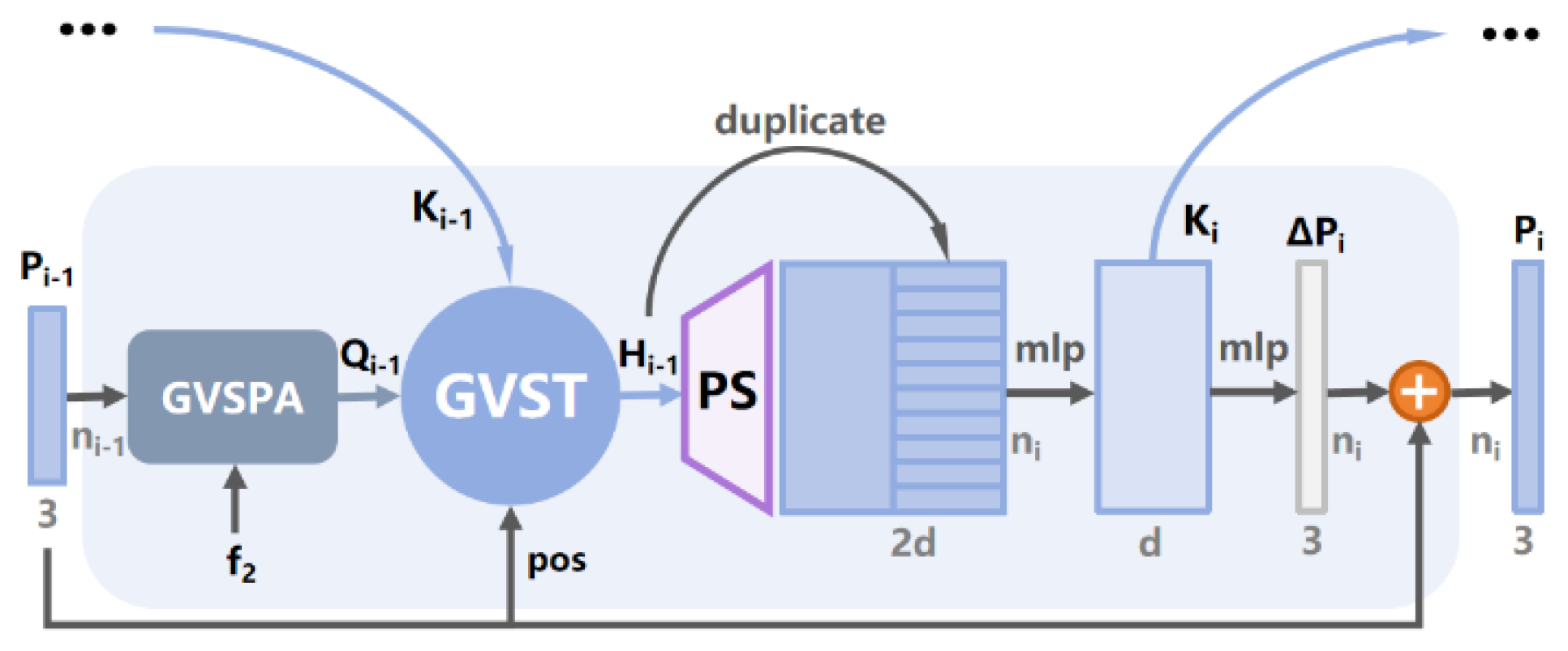
The architecture of SSPD. Here, d is the number of point feature channels, n is the number of points, PS is the point-wise splitting operation, and ⊕ represents element-wise addition.
Figure 3.
The architecture of SSPD. Here, d is the number of point feature channels, n is the number of points, PS is the point-wise splitting operation, and ⊕ represents element-wise addition.
Figure 4.
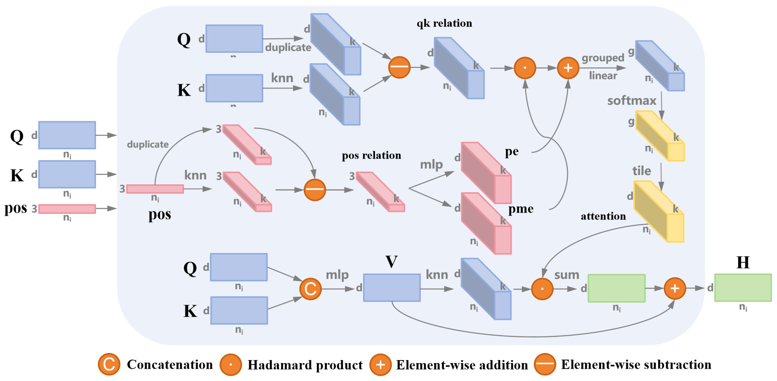
Grouped Vector Skip-Transformer. In the figure, “pos” represents the coordinates of the input points, “pe” stands for the position embedding, “pme” stands for the position multiplication embedding, d denotes the dimension of the point features, ni represents the number of points, k represents the number of nearest neighbors, and g represents the number of groups.
Figure 5.
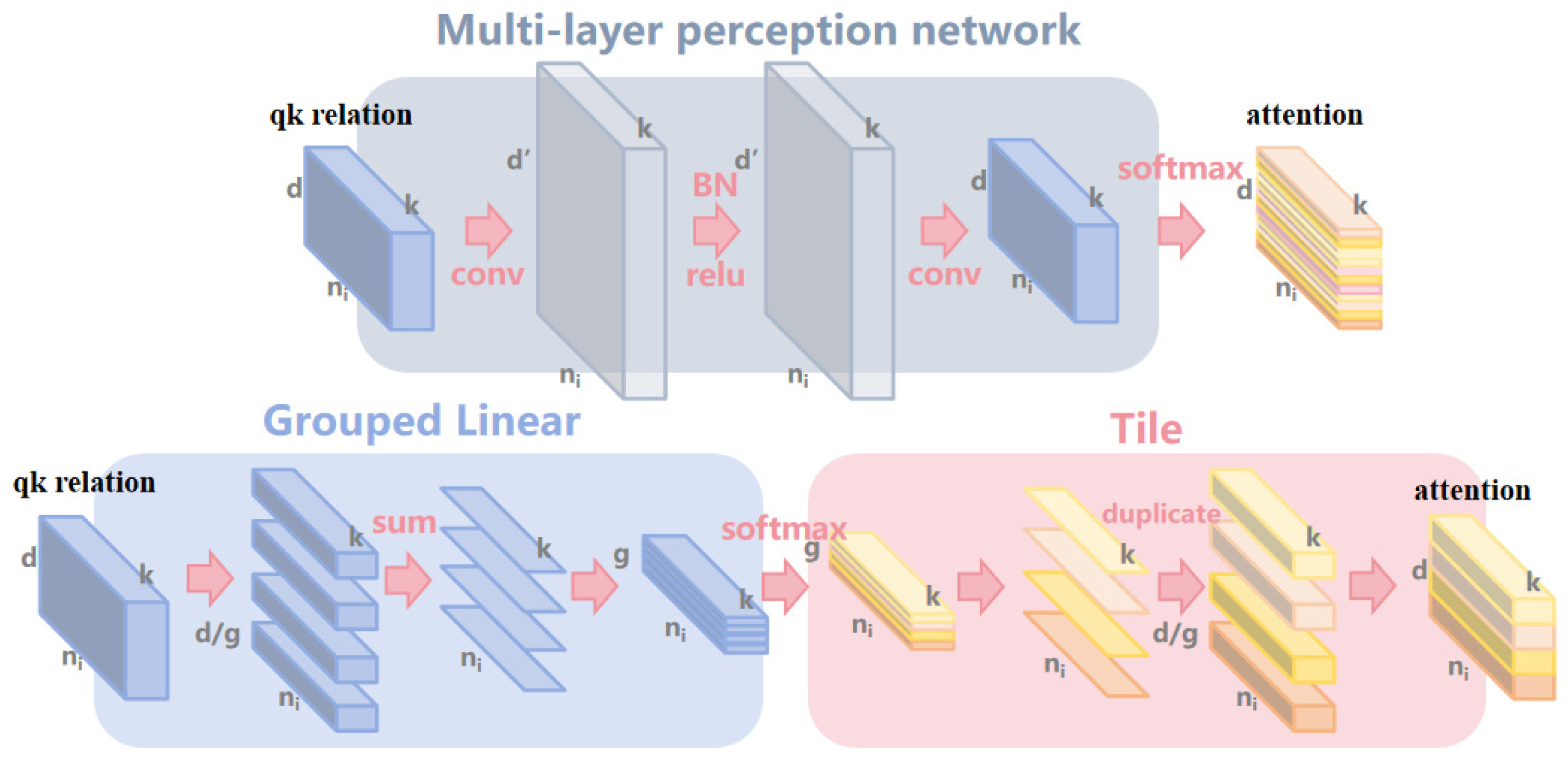
Vector Attention vs. Grouped Vector Attention. The upper part represents traditional vector attention, while the lower part represents Grouped Vector Attention with a group number g = 4. “Conv” denotes the convolutional layer, “bn” stands for batch normalization, ni represents the number of points, and k represents the number of nearest neighbors.
Figure 6.
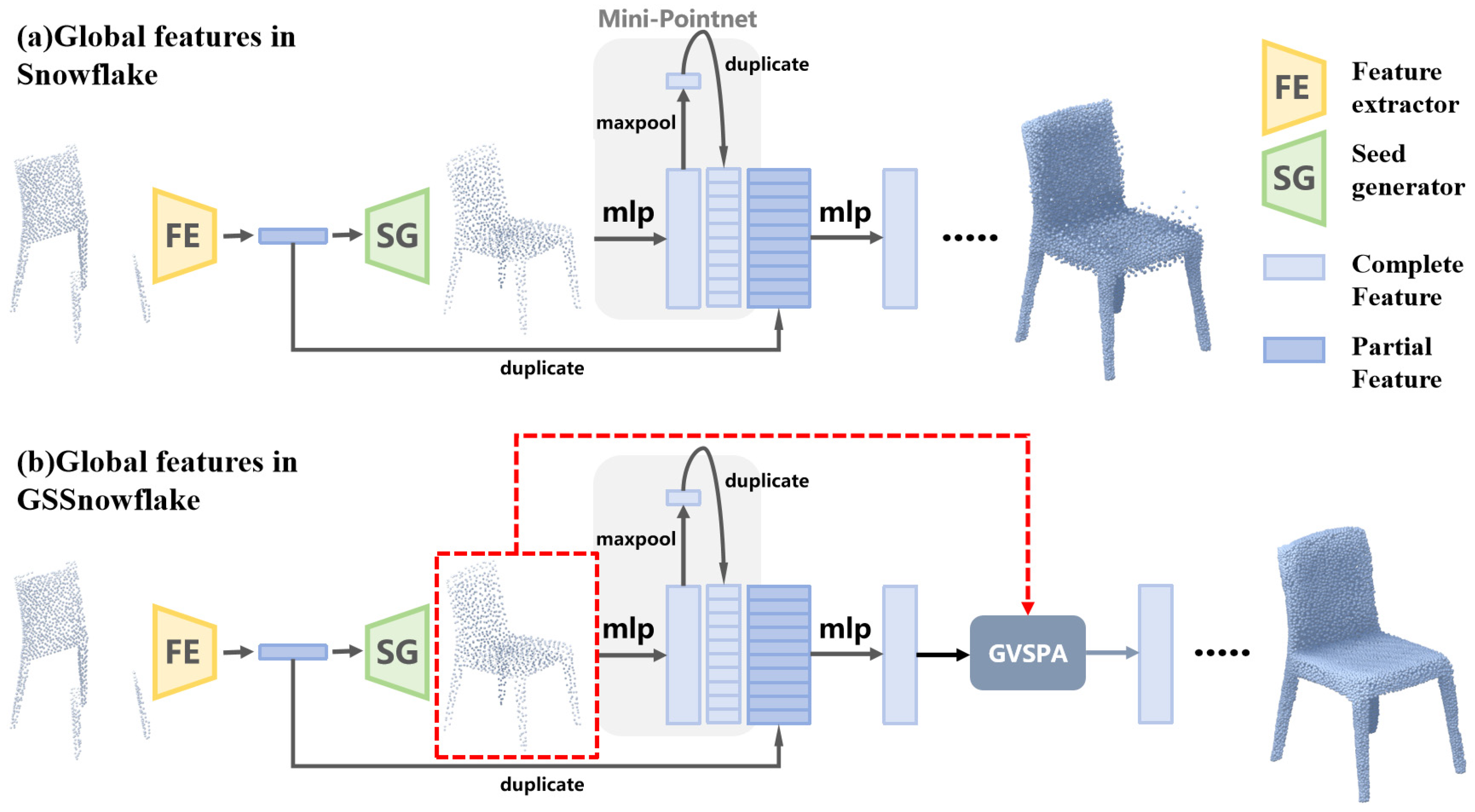
Global feature capture process, taking the first SPD/SSPD as an example and omitting the subsequent point generation process. (a) The global feature capture process in the Snowflake method, which only uses a mini PointNet to capture complete features, resulting in some noise points in the point cloud completion. (b) The global feature capture process in the GSSnowflake method, which uses GVSPA to recapture complete shape features and enhances features using the attention mechanism, resulting in fewer noise points in the point cloud completion.
Figure 7.
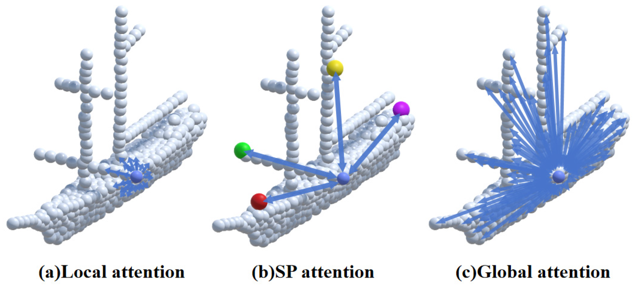
Comparison of local attention, SP attention, and global attention. (a) Local attention calculates attention weights among points within a local region. (b) Self-positioning point attention calculates attention weights only among SP points (colored points in the figure, assuming there are only four SP points). (c) Global attention calculates attention weights among all points.
Figure 8.
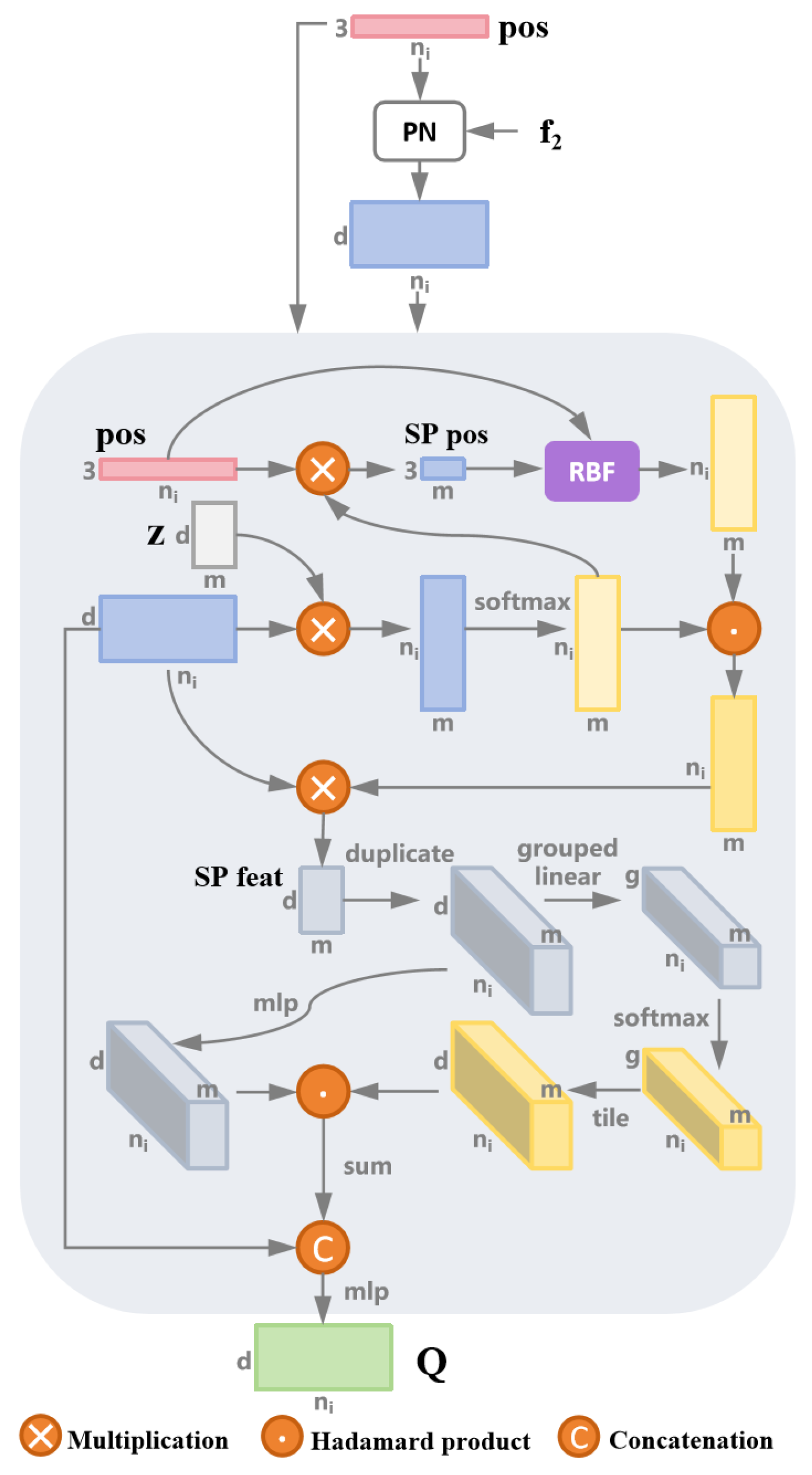
Grouped Vector Self-Positioning Point-based Attention (GVSPA) detailed structure. Here, m represents the number of SP points, “SP pos” represents the coordinates of SP points, “SP feat” represents the features of SP points, RBF (Radial Basis Function) measures spatial similarity, and PN stands for mini PointNet.
Figure 9.
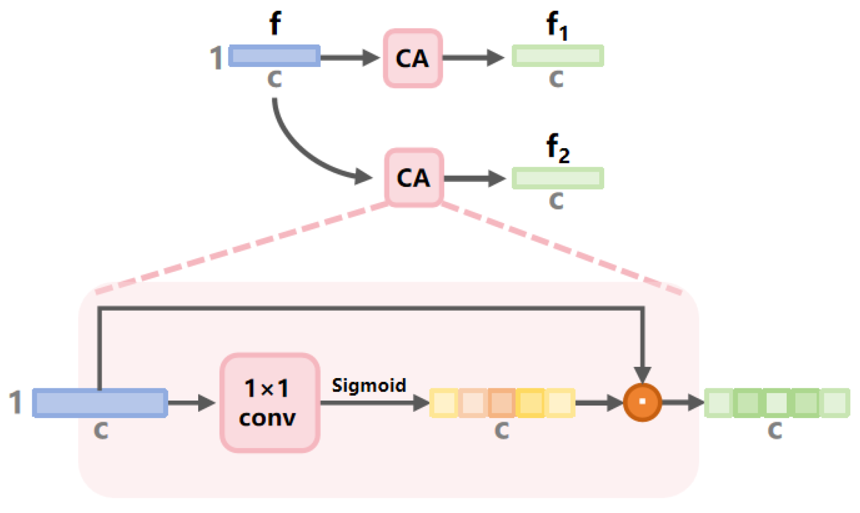
The architecture of the CA module. C represents the number of channels in the global feature vector, and ⊙ denotes the element-wise multiplication.
Figure 9.
The architecture of the CA module. C represents the number of channels in the global feature vector, and ⊙ denotes the element-wise multiplication.
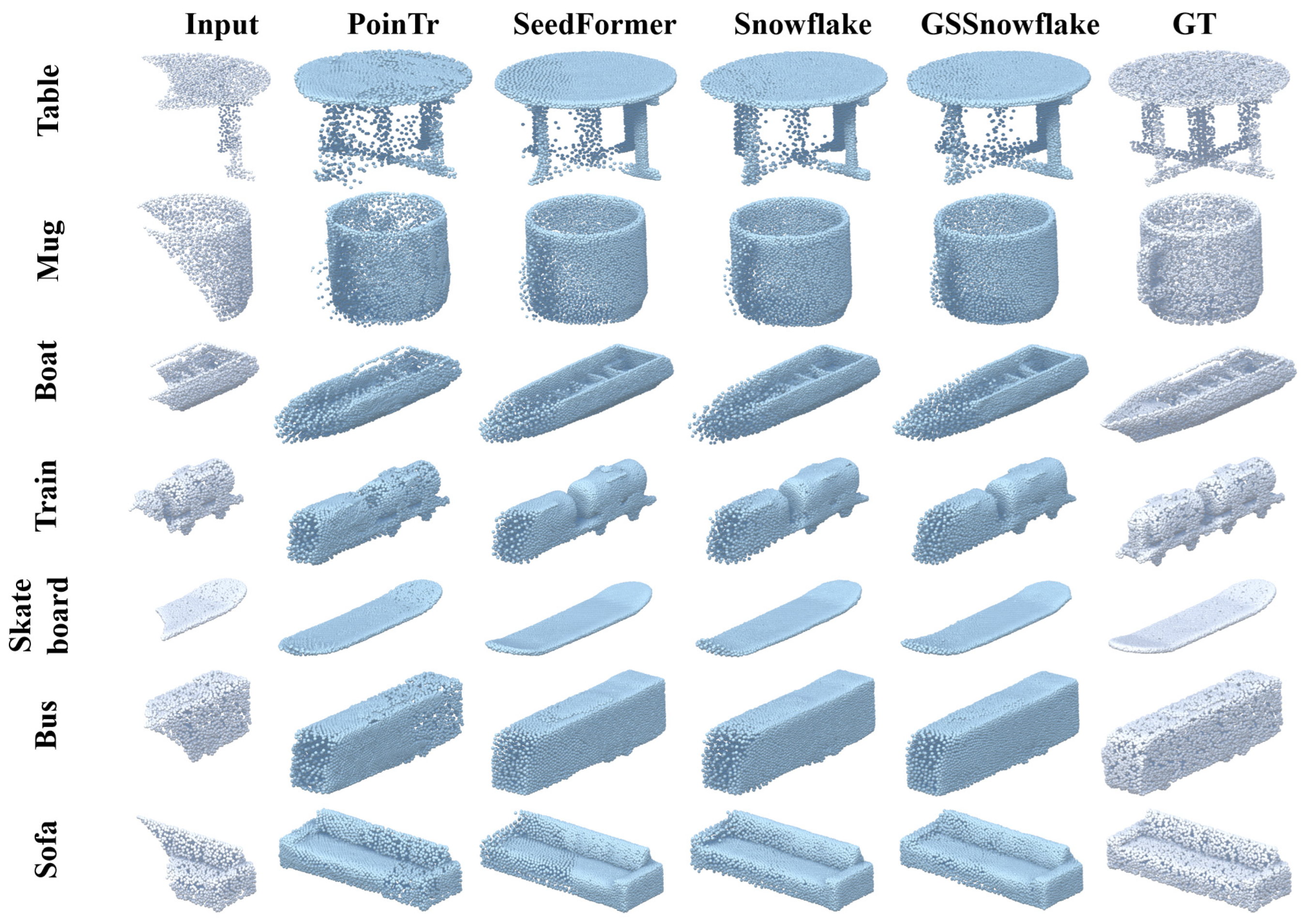
Figure 10.
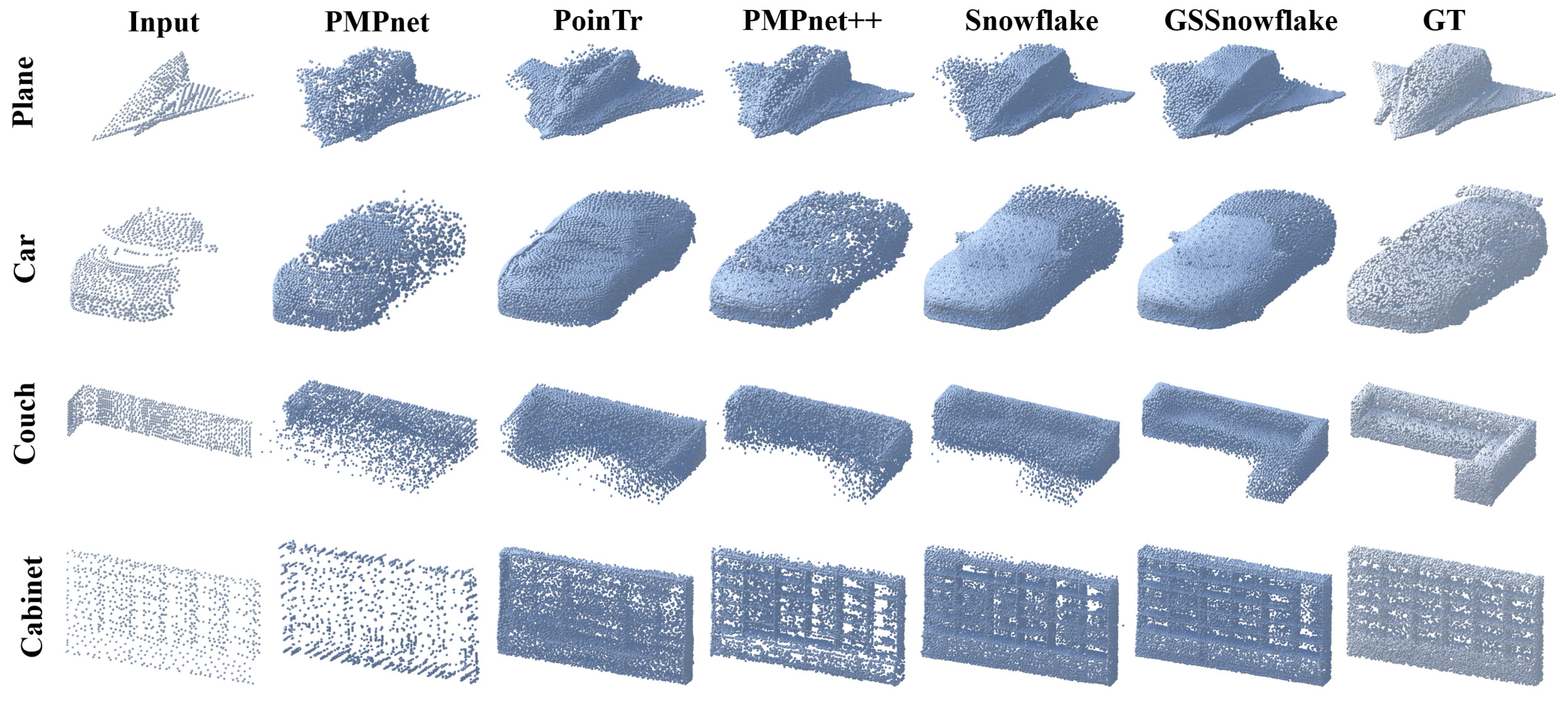
Visual comparison on PCN dataset.
Figure 10.
Visual comparison on PCN dataset.
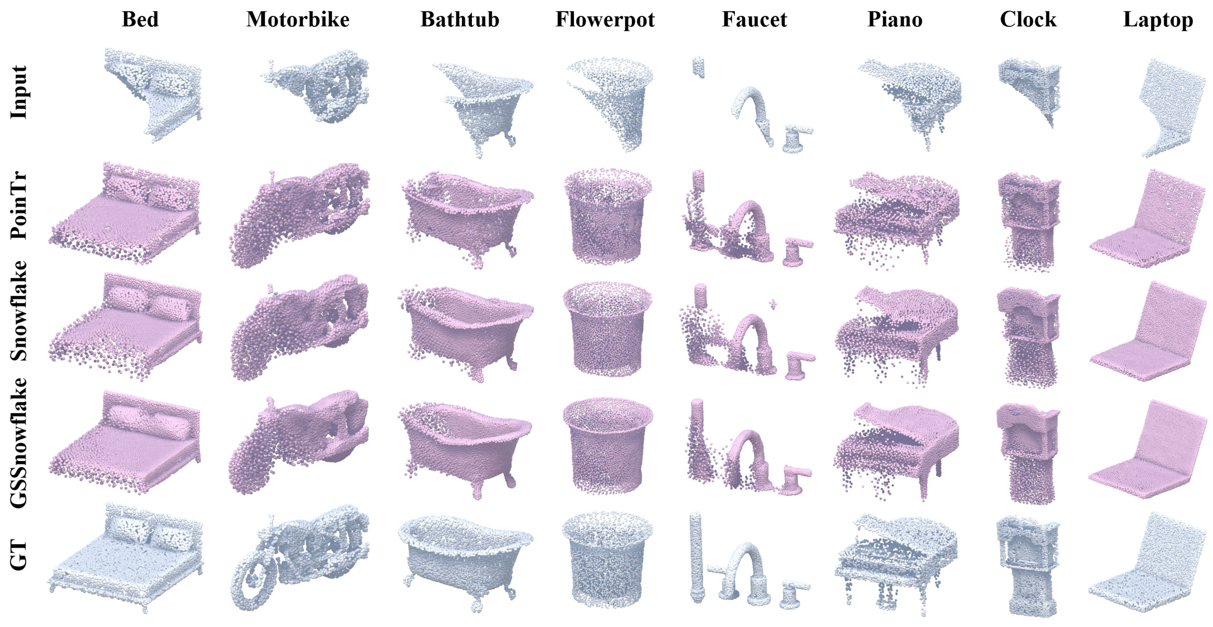
Figure 11.
Visual comparison on ShapeNet-55 dataset.
Figure 11.
Visual comparison on ShapeNet-55 dataset.
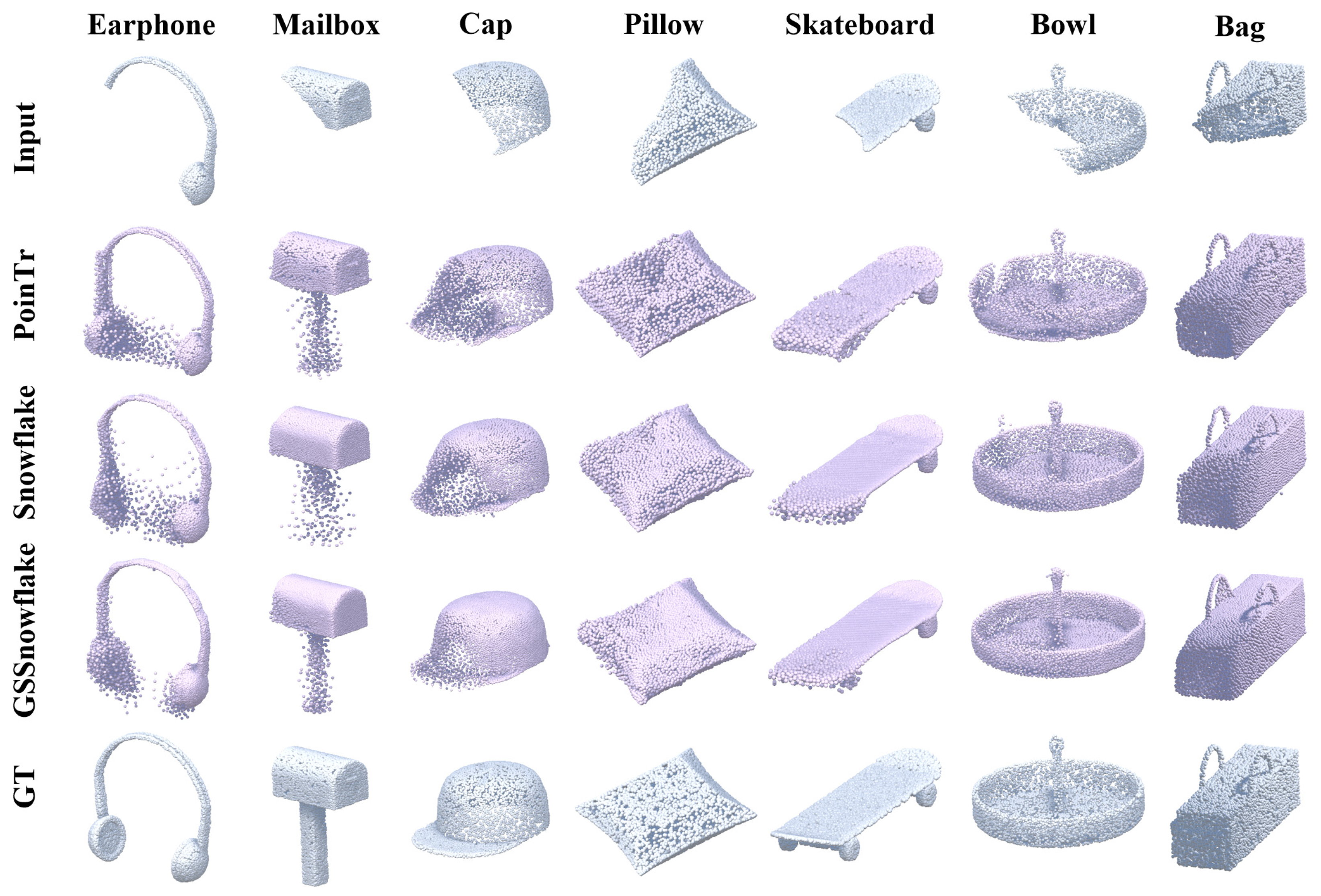
Figure 12.
Visual comparison on ShapeNet-34 dataset.
Figure 12.
Visual comparison on ShapeNet-34 dataset.
Figure 13.
Visual comparison on ShapeNet-unseen21 dataset.
Figure 13.
Visual comparison on ShapeNet-unseen21 dataset.
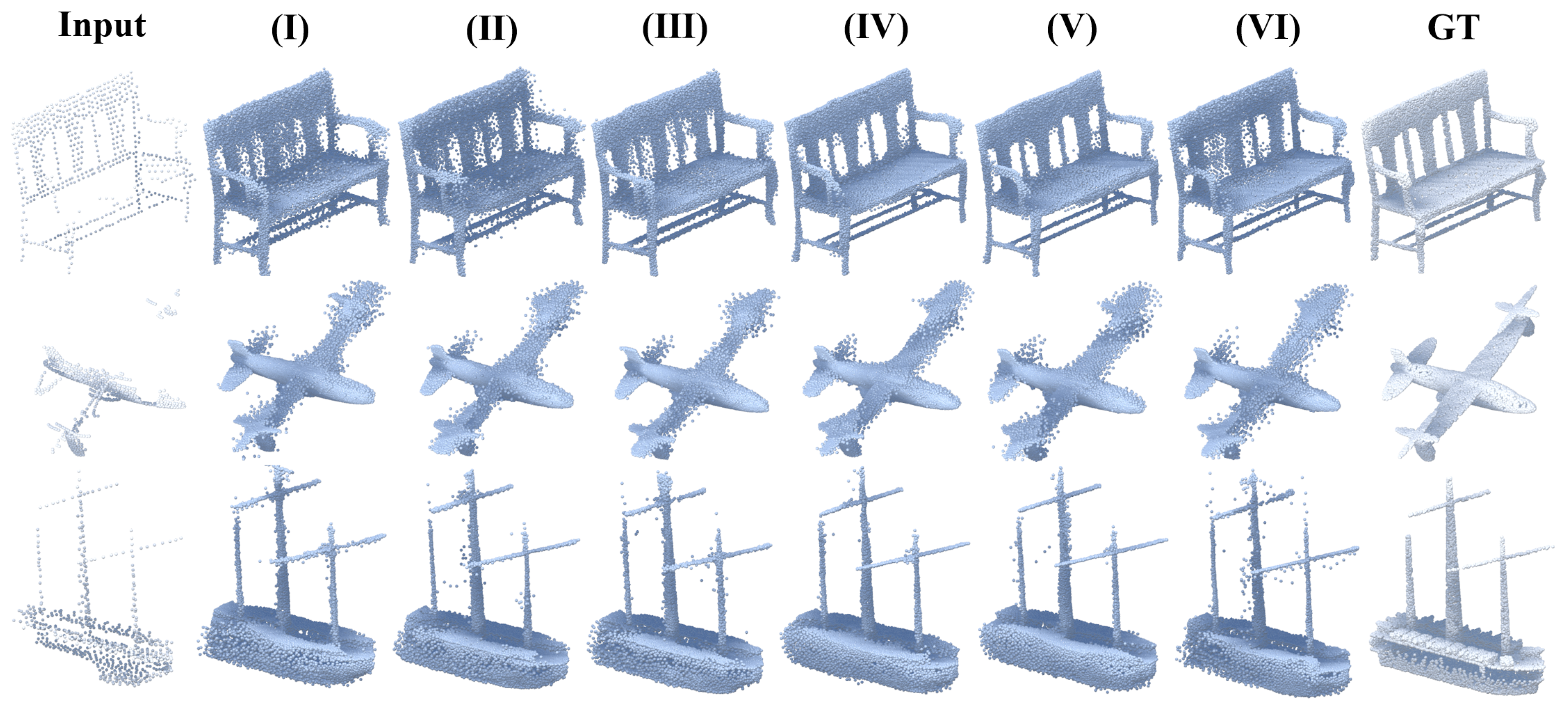
Figure 14.
Visualization of the effect of vector attention grouping quantity.
Figure 14.
Visualization of the effect of vector attention grouping quantity.
Figure 15.
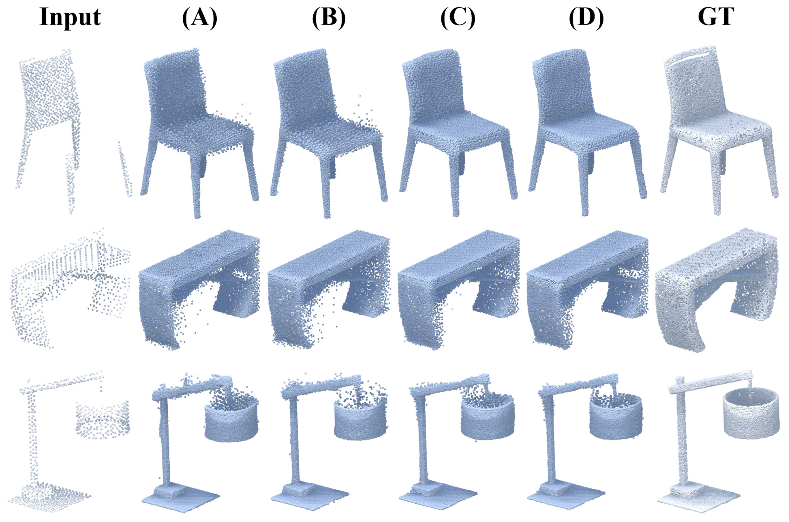
Visual comparison of module design ablation. A denotes the baseline: SnowflakeNet, B indicates the addition of the GVST module to the baseline, C involves incorporating both the GVST and GVSPA modules, and D represents the integration of the GVST, GVSPA, and CA modules together.
Figure 15.
Visual comparison of module design ablation. A denotes the baseline: SnowflakeNet, B indicates the addition of the GVST module to the baseline, C involves incorporating both the GVST and GVSPA modules, and D represents the integration of the GVST, GVSPA, and CA modules together.
Figure 16.
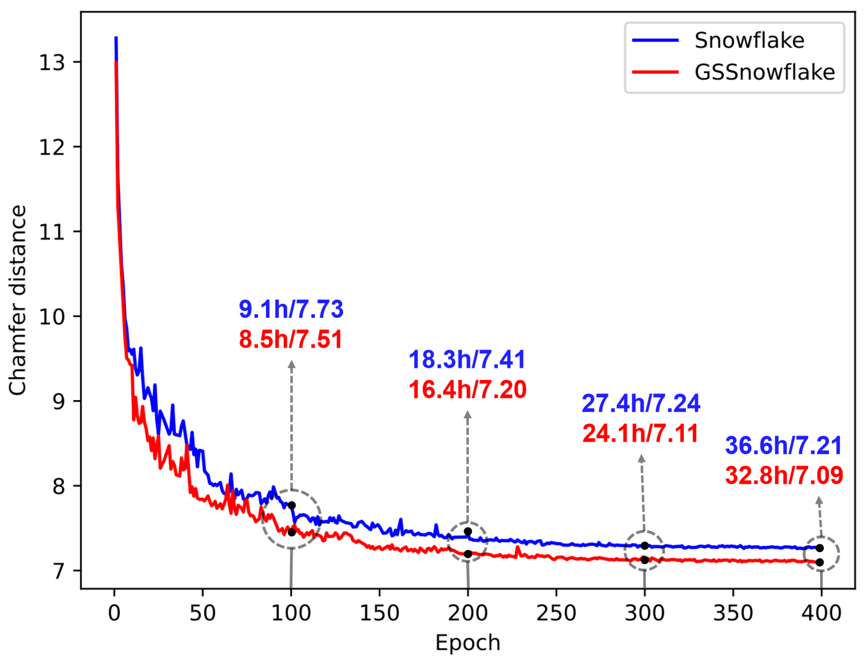
Comparison of training efficiency between Snowflake and GSSnowflake. The number before the “/” represents the time required to train up to the current epoch, measured in hours. The number after the “/” indicates the current average Chamfer Distance.
Figure 16.
Comparison of training efficiency between Snowflake and GSSnowflake. The number before the “/” represents the time required to train up to the current epoch, measured in hours. The number after the “/” indicates the current average Chamfer Distance.
Table 1.
Point cloud completion on PCN dataset in terms of per-point L1 Chamfer distance ×103 (lower is better). Bold indicates optimal performance.
Table 1.
Point cloud completion on PCN dataset in terms of per-point L1 Chamfer distance ×103 (lower is better). Bold indicates optimal performance.
| Methods | Avg | Plane | Cab. | Car | Chair | Lamp | Couch | Table | Boat |
|---|
| PCN [6] | 9.64 | 5.50 | 22.70 | 10.63 | 8.70 | 11.00 | 11.34 | 11.68 | 8.59 |
| GRNet [5] | 8.83 | 6.45 | 10.37 | 9.45 | 9.41 | 7.96 | 10.51 | 8.44 | 8.04 |
| PMP-Net [9] | 8.66 | 5.50 | 11.10 | 9.62 | 9.47 | 6.89 | 10.74 | 8.77 | 7.19 |
| PoinTr [7] | 8.38 | 4.75 | 10.47 | 8.68 | 9.39 | 7.75 | 10.93 | 7.78 | 7.29 |
| PMP-Net++ [10] | 7.56 | 4.39 | 9.96 | 8.53 | 8.09 | 6.06 | 9.82 | 7.17 | 6.52 |
| GTNet [11] | 7.15 | 4.17 | 9.33 | 8.38 | 7.66 | 5.49 | 9.44 | 6.69 | 6.07 |
| Snowflake [17] | 7.21 | 4.50 | 9.29 | 8.16 | 7.66 | 6.15 | 9.06 | 6.47 | 6.37 |
| GSSnowflake (Ours) | 7.09 | 4.32 | 9.22 | 8.06 | 7.54 | 6.17 | 8.65 | 6.41 | 6.33 |
Table 2.
Point cloud completion on the ShapeNet-55 dataset in terms of the L2 Chamfer distance ×104 (lower is better) and F-Score@1% (higher is better) metric. We report the detailed results for each method in 10 categories. CD-S, CD-M, and CD-H denote the CD results under the three difficulty levels of Simple, Moderate, and Hard. Bold indicates optimal performance.
| Methods | Table | Chair | Plane | Car | Sofa | Birdhouse | Bag | Remote | Keyboard | Rocket | CD-S | CD-M | CD-H | CD-Avg | F1 |
|---|
| PCN [6] | 21.3 | 22.9 | 10.2 | 18.5 | 20.6 | 45.0 | 28.6 | 13.3 | 8.9 | 13.2 | 19.4 | 19.6 | 40.8 | 26.6 | 0.133 |
| GRNet [5] | 16.3 | 18.8 | 10.2 | 16.4 | 17.2 | 29.7 | 20.6 | 10.9 | 8.9 | 10.3 | 13.5 | 17.1 | 28.5 | 19.7 | 0.238 |
| PoinTr [7] | 8.1 | 9.5 | 4.4 | 9.1 | 7.9 | 18.6 | 9.3 | 5.3 | 3.8 | 5.7 | 5.8 | 8.8 | 17.9 | 10.9 | 0.464 |
| ProxyFormer [12] | 7.0 | 8.3 | 3.4 | 7.8 | 6.9 | - | - | - | - | - | 4.9 | 7.5 | 15.5 | 9.3 | 0.483 |
| SeedFormer [8] | 7.2 | 8.1 | 4.0 | 8.9 | 7.1 | - | - | - | - | - | 5.0 | 7.6 | 14.9 | 9.2 | 0.472 |
| GTNet [11] | 7.1 | 8.8 | 4.2 | 8.5 | 7.5 | 16.1 | 8.7 | 4.8 | 3.3 | 5.0 | 4.5 | 6.6 | 13.0 | 8.0 | 0.543 |
| Snowflake [17] | 8.3 | 8.2 | 4.2 | 8.1 | 7.9 | 12.4 | 8.0 | 6.1 | 3.8 | 5.9 | 5.2 | 7.3 | 12.5 | 8.3 | 0.457 |
| Ours | 7.7 | 8.0 | 3.9 | 8.0 | 7.7 | 17.2 | 6.8 | 9.3 | 3.0 | 7.1 | 4.9 | 7.0 | 12.1 | 8.0 | 0.478 |
Table 3.
Point cloud completion on the ShapeNet-34/21 dataset in terms of the L2 Chamfer distance ×104 (lower is better) and F-Score@1% (higher is better) metric. CD-S, CD-M, and CD-H denote the CD results under the three difficulty levels of Simple, Moderate, and Hard. Bold indicates optimal performance.
| Methods | 34 Seen Categories | 21 Unseen Categories |
|---|
| CD-S | CD-M | CD-H | CD-Avg | F1 | CD-S | CD-M | CD-H | CD-Avg | F1 |
|---|
| PCN [6] | 18.7 | 18.1 | 29.7 | 22.2 | 0.154 | 31.7 | 30.8 | 52.9 | 38.5 | 0.101 |
| GRNet [5] | 12.6 | 13.9 | 25.7 | 17.4 | 0.251 | 18.5 | 22.5 | 48.7 | 29.9 | 0.216 |
| PoinTr [7] | 7.6 | 10.5 | 18.8 | 12.3 | 0.421 | 10.4 | 16.7 | 34.4 | 20.5 | 0.384 |
| GTNet [11] | 5.1 | 7.3 | 14.0 | 8.8 | 0.511 | 7.8 | 12.2 | 25.6 | 15.2 | 0.467 |
| ProxyFormer [12] | 4.4 | 6.7 | 13.3 | 8.1 | 0.466 | 6.0 | 11.3 | 25.4 | 14.2 | 0.415 |
| Snowflake [17] | 5.1 | 7.1 | 12.1 | 8.1 | 0.414 | 7.6 | 12.3 | 25.5 | 15.1 | 0.372 |
| Ours | 5.0 | 6.8 | 11.7 | 7.8 | 0.428 | 7.3 | 11.7 | 24.4 | 14.4 | 0.391 |
Table 4.
The effect of the number of vector attention groups. We reported a performance comparison under different group numbers. We provide the Chamfer distances metric of all categories in the PCN dataset (CD-Avg).
Table 4.
The effect of the number of vector attention groups. We reported a performance comparison under different group numbers. We provide the Chamfer distances metric of all categories in the PCN dataset (CD-Avg).
| ID | gPT | gGVST | gGVSPA | CD-Avg |
|---|
| I | 4 | 4 | 4 | 7.52 |
| II | 8 | 8 | 8 | 7.37 |
| III | 8 | 16 | 16 | 7.25 |
| IV | 16 | 32 | 32 | 7.09 |
| V | 32 | 32 | 32 | 7.11 |
| VI | - | - | - | 7.21 |
Table 5.
Module design ablation. We report theoretical computation costs (FLOPs) and the number of parameters (Params) of different designs. We also provide the Chamfer distances metric of all categories in the PCN dataset (CD-Avg).
Table 5.
Module design ablation. We report theoretical computation costs (FLOPs) and the number of parameters (Params) of different designs. We also provide the Chamfer distances metric of all categories in the PCN dataset (CD-Avg).
| ID | GVST | GVSPA | CA | CD-Avg | Params | FLOPs |
|---|
| A | | | | 7.21 | 18.58 M | 5.78 G |
| B | √ | | | 7.20 | 18.19 M | 5.09 G |
| C | √ | √ | | 7.12 | 18.26 M | 5.25 G |
| D | √ | √ | √ | 7.09 | 18.26 M | 5.26 G |
Table 6.
The effect of module embedding depth. We report theoretical computation costs (FLOPs) and the number of parameters (Params) of different designs. We also provide the Chamfer distances metric of all categories in the PCN dataset (CD-Avg).
Table 6.
The effect of module embedding depth. We report theoretical computation costs (FLOPs) and the number of parameters (Params) of different designs. We also provide the Chamfer distances metric of all categories in the PCN dataset (CD-Avg).
| ID | dPT | dGVST/dST | dGVSPA | CD-Avg | Params | FLOPs |
|---|
| A | 64 | 64 | 64 | 7.09 | 18.26 M | 5.26 G |
| B | 128 | 128 | 128 | 7.08 | 18.49 M | 5.84 G |
| C | 64 | 64 | - | 7.21 | 18.58 M | 5.78 G |
| D | 128 | 128 | - | 7.23 | 19.15 M | 7.76 G |
Table 7.
Complexity analysis. We report theoretical computation costs (FLOPs) and the number of parameters (Params). We also provide the Chamfer distances metric of all categories in ShapeNet55 (CD55), ShapeNet34 (CD34), ShapeNet-unseen21 (CD21), and PCN benchmark (CDPCN) as references. Bold indicates optimal performance.
| Methods | Params | FLOPs | CDPCN | CD55 | CD34 | CD21 |
|---|
| GRNet [5] | 76.71 M | 20.43 G | 8.83 | 19.7 | 17.4 | 29.9 |
| PMP-Net [9] | 5.44 M | 9.61 G | 8.66 | - | - | - |
| PoinTr [7] | 30.88 M | 5.94 G | 8.38 | 10.9 | 12.3 | 20.5 |
| PMP-Net++ [10] | 5.89 M | 10.85 G | 7.56 | - | - | - |
| GTNet [11] | 11.20 M | 7.64 G | 7.15 | 8.0 | 8.8 | 15.2 |
| Snowflake [17] | 18.58 M | 5.78 G | 7.21 | 8.3 | 8.1 | 15.1 |
| Ours | 18.26 M | 5.26 G | 7.09 | 8.0 | 7.8 | 14.4 |
Table 8.
Model efficiency. We demonstrated the latency and memory during training and inference to compare model efficiency. Bold indicates optimal performance.
Table 8.
Model efficiency. We demonstrated the latency and memory during training and inference to compare model efficiency. Bold indicates optimal performance.
| Method | Training | Inference |
|---|
| Latency | Memory | Latency | Memory |
|---|
| Snowflake [17] | 170 ms | 5.6 G | 80 ms | 2.1 G |
| Ours | 156 ms | 5.2 G | 71 ms | 1.8 G |


