Article

RGBTSDF: An Efficient and Simple Method for Color Truncated Signed Distance Field (TSDF) Volume Fusion Based on RGB-D Images

1
School of Remote Sensing and Information Engineering, Wuhan University, Wuhan 430079, China
2
Wuhan Ruler Technology, Wuhan 430079, China
3
Hubei Luojia Laboratory, Wuhan 430079, China
*
Author to whom correspondence should be addressed.
These authors contributed equally to this work.
Remote Sens. 2024, 16(17), 3188; https://doi.org/10.3390/rs16173188
Submission received: 1 July 2024 / Revised: 17 August 2024 / Accepted: 27 August 2024 / Published: 29 August 2024
(This article belongs to the Special Issue New Insight into Point Cloud Data Processing)

Abstract

:
RGB-D image mapping is an important tool in applications such as robotics, 3D reconstruction, autonomous navigation, and augmented reality (AR). Efficient and reliable mapping methods can improve the accuracy, real-time performance, and flexibility of sensors in various fields. However, the currently widely used Truncated Signed Distance Field (TSDF) still suffers from the problem of inefficient memory management, making it difficult to directly use it for large-scale 3D reconstruction. In order to address this problem, this paper proposes a highly efficient and accurate TSDF voxel fusion method, RGBTSDF. First, based on the sparse characteristics of the volume, an improved grid octree is used to manage the whole scene, and a hard coding method is proposed for indexing. Second, during the depth map fusion process, the depth map is interpolated to achieve a more accurate voxel fusion effect. Finally, a mesh extraction method with texture constraints is proposed to overcome the effects of noise and holes and improve the smoothness and refinement of the extracted surface. We comprehensively evaluate RGBTSDF and similar methods through experiments on public datasets and the datasets collected by commercial scanning devices. Experimental results show that RGBTSDF requires less memory and can achieve real-time performance experience using only the CPU. It also improves fusion accuracy and achieves finer grid details.

1. Introduction

The Truncated Signed Distance Function (TSDF) [1,2] is a common implicit surface representation for computer graphics and computer vision applications that can construct the surface information of a scene or object, filter sensor noise, and create meshes. It is widely used in fields such as robots, drones, and three-dimensional scanning. TSDF can be used in most devices with depth sensors, such as RGB-D cameras, 3D lidar, etc. Among them, 3D lidar has good accuracy, but it is expensive and difficult to carry. The RGB-D camera simultaneously captures the texture and geometric information of the observed scene in the form of color and depth image streams at a real-time frame rate. It has the characteristics of small size, low cost, portability, and easy operation. Therefore, it is widely used in 3D reconstruction [3,4] SLAM map construction [5]. We are focusing on exploring the mapping of RGB-D images.
In RGB-D image mapping, the camera can provide an RGB-D data stream of more than 300,000 pixels at a rate of 30 frames per second. Therefore, the mapping algorithm must process the data at a rate close to, or even faster than, this speed to achieve the real-time goal. If the processing speed is too slow, it will cause large delays in data updates, which will affect the spatial overlap rate of the data, resulting in a loss of camera tracking accuracy. Some TSDF fusion systems rely on accelerators [6,7,8], such as GPUs, but it will increase the cost of the equipment and limit the application in certain consumer-level scenarios. Therefore, there is still a need to develop an efficient and lightweight mapping algorithm to improve the efficiency of RGBD 3D reconstruction.
The high-rate data acquisition of RGB-D cameras also poses significant challenges for real-time data management [9,10]. Real-time fusion mapping is a highly dynamic process, and due to the limited size of the field of view, it is often necessary to move the camera to observe different parts of the scene. Therefore, it is necessary to add newly observed surfaces and update those already observed in a high-frequency manner. When building high-resolution scenes in large areas, how to effectively manage data and improve the efficiency of memory usage is also a question worth addressing.
In addition, although the currently commonly used TSDF data fusion technology can use weighted averaging to eliminate most of the noise, it will also smooth out many high-frequency geometric details, resulting in geometric errors in the reconstructed model. As a result, the reconstructed geometric model cannot meet the high-quality geometric requirements. In addition, the classical TSDF [11,12] needs to discretize the data at many points during the entire processing. Its quantization error will also affect the accuracy of the reconstructed mesh. Therefore, how to improve the accuracy of TSDF fusion to obtain more geometric details still needs to be explored.
To solve the above problems, we propose a TSDF voxel fusion method for large scenes with high efficiency and higher accuracy. First, based on the sparse characteristics of volume, an improved octree is used to manage the entire scene, called a grid octree. A grid octree has a fixed depth and can effectively store and operate sparse volume data. In addition, a hard coding method is proposed for indexing and quickly querying the coordinates of a certain voxel in the entire tree, which significantly reduces its memory footprint and speeds up querying. Secondly, to overcome the loss of sub-pixel accuracy caused by the rounding of pixel coordinate values during the depth map fusion process, the depth map is interpolated to achieve a more accurate voxel fusion effect. Finally, a smooth mesh extraction method with texture constraints is proposed to overcome the effects of noise and holes and improve the smoothness and refinement of the extracted surface.
The main contributions of this paper can be summarized as follows: A more efficient and accurate mapping system is proposed and made open-source. There is no limit to the size of the mapping environment and it is faster than the state-of-the-art systems using only the CPU. Furthermore, our system allows for more accurate surface reconstruction.

2. Related Work

2.1. Efficiency Optimization of TSDF

TSDF is a commonly used mapping technique. Curless et al. [2] propose an algorithm that uses signed distance functions to accumulate surface information into voxel grids. The surface is implicitly represented as the zero crossing of the aggregated signed distance function, which is referred to as the volume method. On this basis, KinectFusion [1] first implements a real-time frame rate reconstruction algorithm based on RGB-D cameras, but it uses a fixed-size voxel grid to represent the entire space instead of densely reconstructing only near the observation surface. This results in a waste of memory space. To solve this problem, many scholars have successively explored sparse data structures to build systems, such as the octree data structure [13,14] and hash table [10,15]. The main idea is to only perform dense reconstruction near the observation surface and discard empty positions. The octree is essentially an adaptive voxel grid that only allocates high-resolution cells near the surface to save memory. For example, Octomap [9] introduces probabilistic updating into the octree and introduces a node compression function, which can effectively reduce memory consumption. However, to insert a high line count such as 128-line LiDAR without any data volume reduction processing, using Octomap will be very slow. Fuhrmann [16] introduces a hierarchical SDF structure using an adaptive octree-like data structure to provide different spatial resolutions. The octree data structure has low parallelism, so its performance is severely limited. Nießner et al. [10] propose voxel hashing as a representation of an almost infinite scene by a regular grid of smaller voxel blocks of predefined size and resolution, whose spatial locations are addressed by a spatial hash function. Only voxel blocks that contain geometric information are instantiated and the corresponding indexes are stored in the linearized spatial hash. This strategy significantly reduces memory consumption and allows efficient access, insertion, and deletion of data in the hash table with O (1) time complexity. Based on this minimized memory footprint and efficient computational capabilities, Google applies the hash mapping method to mobile phones [17]. Additionally, it can easily stream reconstructed parts from the core to support high resolution and extremely fast runtime performance. Li et al. [6] propose a structured skip table method to increase the number of voxels that each entry of the hash table can accommodate, thereby increasing the scale of the three-dimensional space that a hash table of the same size can represent. However, the hash function used in this method has a high collision probability. If the number of collisions is large, it will seriously slow down the efficiency of the algorithm and increase the risk of memory overflow.
While these methods alleviate some of the memory pressure, challenges remain. In the context of real-time scene reconstruction, most approaches rely heavily on the processing power of modern GPUs and are limited by predefined volumes and resolutions. However, the powerful GPUs are expensive, and it would be a breakthrough if they could be used on CPUs and in real time. Therefore, much research has been devoted to speeding up these algorithms on CPUs and even mobile devices, while the application of high-resolution 3D reconstruction remains unchanged. Steinbrücker et al. [13] use a multi-resolution data structure to represent the scene on the CPU, including an incremental mesh output process to achieve real-time accumulation. However, the method can only be set to a few fixed resolutions and the speed is slow. Vizzo et al. [18] use the OpenVDB hierarchical structure [19] to manage the memory, which improves the fusion speed and accuracy, and forms a unified and complete mapping framework. Voxblox [20] uses voxel hashing, where the mapping between voxel positions in the map and their positions in memory is stored in a hash table, which can achieve a faster query speed than octree maps. However, this system depends on ROS and is not easy to extend.

2.2. Geometry Optimization of TSDF

After the TSDF model is established, surface extraction can be performed to generate meshes for visualization or other downstream applications. In order to generate high-quality mesh, Vizzo et al. [21] use poisson surface reconstruction [22] to construct the mesh. Poisson reconstruction can obtain accurate results, but it is generally processed offline and is not a true incremental method, or applicable to real-time systems. In TSDF real-time systems, the Marching Cubes algorithm [23] is often used to extract surfaces. The algorithm uses a lookup table to determine the triangle topology within the cell and interpolates between vertices to find the edge intersections of isosurfaces and cubes of voxels very quickly. At present, many researchers have realized the real-time construction of TSDF triangular mesh based on this method [24,25]. However, it leads to uneven shapes and sizes of triangles. To solve this problem, the marching triangles algorithm proposed by Hilton et al. [26] uses Delaunay triangulation and places vertices according to local surface geometry, thereby generating triangles with more uniform shapes and sizes. In addition, Marching Cubes may also cause the mesh to appear “jaggy” at features (edges or sharp corners), making it unsuitable for processing objects with complex details. To solve this, Kobbelt et al. [27] propose Extended Marching Cubes, which uses feature-sensitive sampling, thereby reducing aliasing effects on features. But this method requires the extraction of grid features, which is more complex. Furthermore, there are also some methods to improve the geometric quality of the 3D reconstruction model by optimizing the depth map or geometric model, such as denoising, completion, interpolation to enhance details, multi-constraint optimization, etc. In terms of depth map optimization, Premebida et al. [28] use bilinear filtering to directly complete the depth map and retain edge smoothing noise. Wu et al. [29] propose a real-time depth map optimization method based on Shape-from-Shading (SFS), which uses the relationship between shading changes and surface normals to optimize the depth map, requiring only a few lighting assumptions. In terms of geometry optimization, Xie et al. [30] first estimate the normal map of the entire model, infer the high-frequency geometric details in the reconstructed model, and then optimize the surface geometry. Zhou et al. [31] propose the Dual Contouring method, which uses the Hermite interpolation data structure to obtain accurate intersection points and normals, construct the isosurface, and use the quadratic error function to generate vertex coordinates and then generate mesh patches.

3. Methodology

Figure 1 illustrates the overall flow of our approach. For the input RGB images and depth images and corresponding camera intrinsic and extrinsic, we first build grid octree and increase the indexing speed of the data by a hard coding index. Based on this, we build the TSDF and improve the accuracy of TSDF fusion by depth map interpolation. Finally, we obtain the reconstructed mesh by the proposed mesh extraction with texture constraints method. In this following section, we will describe the RGBTSDF volume mapping system in detail from four aspects: grid octree data structure, hard coding index method, voxel fusion with depth map interpolation, and mesh extraction with texture constraints.

3.1. Grid Octree

Real-time fusion mapping is a highly dynamic process that often requires the frequent addition of newly observed surfaces and updating of previously observed surfaces to the global surface model. To ensure fast data addition, deletion, modification, and checking, the temporal efficiency of the underlying data structure storing the 3D surface information is strongly required. In addition, spatial efficiency is equally important, and a reasonable data structure can reduce memory usage. In order to manage the scene efficiently, an improved octree structure is proposed in this subsection.
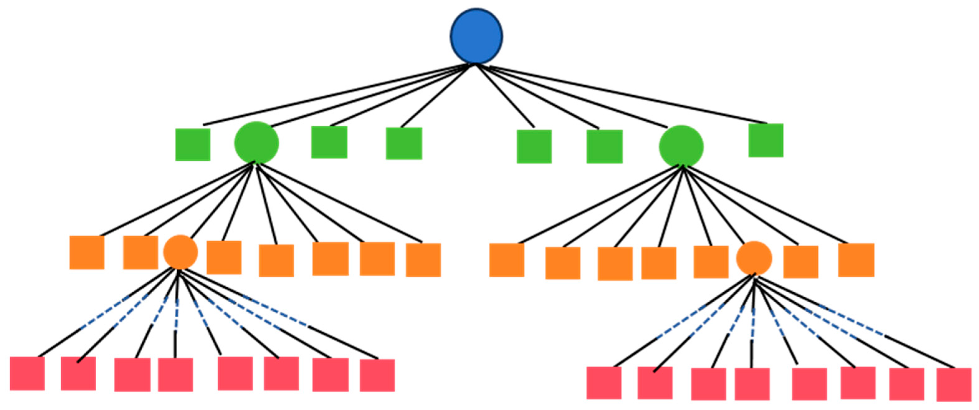
When dealing with sparse data, it is common to use a tree structure, such as an octree. An important reason for using such structures is the almost infinitely sparse representation of the scenario, i.e., there is no need to know in advance the size of the environment to be used. Therefore, it is effectively used in systems where memory and CPU resources are limited. A traditional octree [13,14], as shown in Figure 2, starts from a root node until it reaches a leaf node containing a predefined number of points or sizes. The leaf nodes of an octree can be at any level other than the root node, and thus it is usually very deep, which increases the time complexity of traversing the tree from the root node to the leaf nodes.
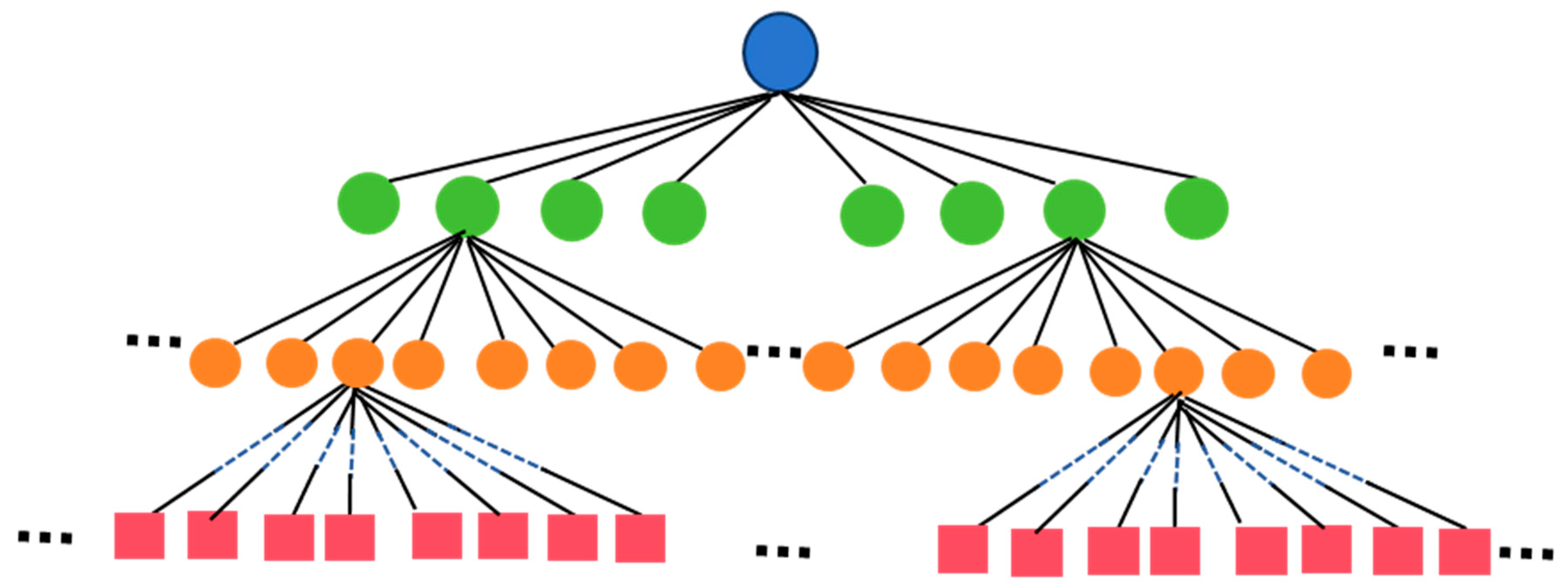
The proposed grid octree data structure is shown in Figure 3. Compared with the octree, the grid octree modifies the octree node construction. All the leaf nodes are in the last layer with large and variable branching factors, which means that the grid octree is highly balanced and very wide, and at the same time, the depth is very shallow. It effectively increases the spatial extent of the data structure that can be represented, while reducing the depth of the tree, thus reducing the time complexity of traversing the tree from the root node to the leaf nodes.
A fixed number of voxels are combined and stored together, which is called a voxel block. During storage, the coordinates of the entire voxel block are defined with the coordinates of the center point, and the coordinates of each voxel can be obtained from the coordinates of the voxel block. The grid octree represents a sparse collection of voxel blocks. Leaf nodes are the smallest units that store voxel blocks and are located at the lowest level of the tree at the same depth as when they are created. The voxel block is divided into voxels along each coordinate axis. The size is set by the user, and we recommend a size of 3, corresponding to an 8 × 8 × 8 block. Setting the node size to a power allows for fast bit operations when traversing the tree. Due to the shallow and fixed depth, accessing the grid octree data structure is more efficient than traversing the octree, and sparse high-resolution voxel blocks can be accessed quickly. In addition, the grid octree allows for dynamic expansion of the spatial domain with almost no scale restrictions, making it well-suited for highly dynamic application scenarios such as real-time 3D reconstruction.

3.2. Hard Coding Index

The indexing speed of data is crucial. Especially for sparse data, optimizing the indexing time directly affects the efficiency of fusion mapping. This subsection introduces a hard coding data indexing method to map data from a high-dimensional space to a one-dimensional space, which can quickly add, delete, and verify data.
A grid octree can represent an almost infinite three-dimensional index space if the precision of the data type and the memory space allow it. However, data indexing, especially for sparse data, is a problem for optimizing the indexing time. Data encoded in a grid octree consist of a value type and a corresponding discrete index (x, y, z). The spatial index specifies the location of its spatial voxel, the data value is associated with each voxel, and the specific meaning of the data value is defined by the user, which can be either 3D point data or directed distance function (TSDF). Most of the existing methods use the hash key [14] for encoding, but hash has low speed and hash conflicts. RGBTSDF uses a hard coding method to encode (x, y, z) discrete values compactly into variables, mapping 3D coordinates onto 1D space, thus significantly reducing its memory footprint and speeding up queries.
Specifically, we hard code the (x, y, z) discrete values into a 64-bit token. As shown in Figure 4, the last 3 × 21 bits encode the coordinate origin of the current leaf node under the global coordinate system of the whole tree, which can be used to derive the global coordinate values of the voxels in the leaf node. The first bit is flexible and can be extended by the user according to their needs. Finally, we implement a large range of scene management with a maximum length of 221. This hard coding method is able to obtain the coordinates of a voxel in the whole tree without indexing its parent node beforehand, which makes the indexing very flexible and avoids additional memory overhead, and the implementation is simple, reliable, and efficient.
The process of inserting voxel data into the grid octree during data access can be described as follows: first, calculate the spatial index coordinates of a voxel in the grid octree according to its position, find the leaf node where it is located in the grid octree, and then store it at the corresponding voxel position in that node. The method of randomly finding data from the grid octree is similar to the above process. The formula is expressed as follows:
I ( x , y , z ) = p = p x / + 0.5 p y / + 0.5 p z / + 0.5 T

3.3. Voxel Fusion with Depth Map Interpolation

During the TSDF calculation process, for each voxel point, its corresponding pixel coordinates (u, v) on the image are calculated based on the position of the current frame and the camera’s intrinsic parameters. In most of the existing methods [14,18], the voxel coordinates (u, v) are directly rounded to correspond to the depth map. However, direct rounding loses the sub-pixel information of the voxel coordinates, resulting in quantization errors and chunk formation, which affects the accuracy of the fusion. In this section, bilinear interpolation is used to calculate the exact surface depth value of (u, v) in the depth map, and then the distance depth from the voxel point to the camera is calculated to obtain the truncated distance value of the current voxel point. The specific procedure is as follows:
Assume that at each timestamp i, the depth camera can capture a depth image D i corresponding to the current viewpoint. The position of a given pixel in the depth image is expressed in terms of homogeneous coordinates as U = [ u , v , 1 ] T , the depth value is expressed as d = D i ( U ) , and its corresponding three-dimensional point in the camera coordinate system is expressed as P = [ x , y , z , 1 ] T . The intrinsic parameter matrix of the depth camera is defined as follows:
K = f x 0 c x 0 f y c y 0 0 1
where f x and f y are the normalized focal lengths of the depth camera on the x and y axes, and c x and c y are the horizontal and vertical coordinates of the camera’s optical center on the imaging plane. The projection equation for mapping pixels from the camera coordinate system to the image coordinate system is as follows:
U = π ( P ) = K x z y z 1 T = x z f x + c x y z f y + c y 1 T
The 3D point cloud P in the camera coordinate system can be back-projected from the pixel point U into the camera coordinate system through the inverse transformation π 1 of the projection equation π:
P = π 1 U = K 1 u v 1 T d = u c x f x d v c y f x d d T
According to the rotation matrix R and translation matrix T of the camera, the conversion relationship between the point P c in the world coordinate system and the pixel point U can be obtained as follows:
U = K R | T P c
The TSDF is associated with the depth measurement by back-projecting the voxel onto the image plane using the camera’s intrinsic matrix. The distance along the direction of the observation ray is calculated as the TSDF according to the above equation, i.e., the corresponding measurement on the depth map minus the z-coordinate value of the voxel. If a voxel is centered at p = ( p x , p y , p z ) and its corresponding pixel coordinate is X = u , v T = π ( p ) , then the TSDF is calculated as follows:
s d f p = ( D ( X ) p z ) 1 + ( p x / p z ) 2 + ( p y / p z ) 2
t s d f p = s d f p / σ   if   s d f p < σ sgn   ( s d f p )
where σ is the truncation threshold. If s d f p is greater than the truncation threshold, the value is set to be −1 or +1 according to the sign function sgn. The truncation distance threshold σ is set because voxels that are very far away from the surface contribute very little to the reconstruction quality and truncating them can reduce memory consumption and improve computational speed. The setting of σ affects the quality of the reconstructed surface. If σ is set too large, some small features on the surface will be smoothed. If σ is smaller than the measured noise level, this will result in isolated components around the reconstructed surface. In addition, the setting of the truncation distance must be combined with the thickness of the reconstructed surface. If the thickness of the surface is less than the width of the truncation zone, the values in the TSDF field measured on opposite sides of the encoded surface will interfere with each other, resulting in the inability to recover the real surface from the field.
However, in most of the existing implementations, since the corresponding pixel coordinates in the depth map are integers, the pixel coordinates at the center of the solved voxel are solved by the projection matrix using U = π ( p ) , i.e., a rounding operation. In direct rounding, the subpixel information of the pixel coordinates is lost, which affects the fusion accuracy. Here, we use bilinear interpolation to obtain the exact depth value corresponding to the pixel coordinates, which effectively improves the details of the fused mesh. The interpolated depth value D ( u , v ) is calculated as follows:
a ^ = a 0 a 1 = u u u u
b ^ = b 0 b 1 = v v v v
D ( u , v ) = a ^ T D u , v D u , v D u , v D u , v b ^ T
D w = b 0 a 0 s D u , v + b 0 a 1 s D u , v + b 1 a 0 s D u , v + b 1 a 1 s D u , v
s d = 0 ,   d = 1 1 ,   d < 1
where ⌊u⌋ and ⌊v⌋ are u and v rounded down, respectively, and ⌈u⌉ and ⌈v⌉ are u and v rounded up, respectively. D w is the weight. The interpolated depth value D ( u , v ) needs to be divided by the weight. Then the calculation formula of sdf is deformed as follows:
s d f p = ( D ( X ) / D w p z ) 1 + ( p x / p z ) 2 + ( p y / p z ) 2
In the process of multi-frame fusion, we only calculate the relevant volume, and quickly query the corresponding volume number by calculating the position of the three-dimensional point of the current frame. The formula for calculating the TSDF value for multi-frame fusion is as follows:
V t x = V t 1 ( x ) + w t x ( v t x V t 1 ( x ) ) W t ( x ) W t x = W t 1 x + w t
where W t ( X ) is the sum of the historical weights of point X, and V t is the weighted mean of the TSDF value. w t is the weight corresponding to the current frame, and v t is the TSDF value of the current frame.

3.4. Mesh Extraction with Texture Constraints

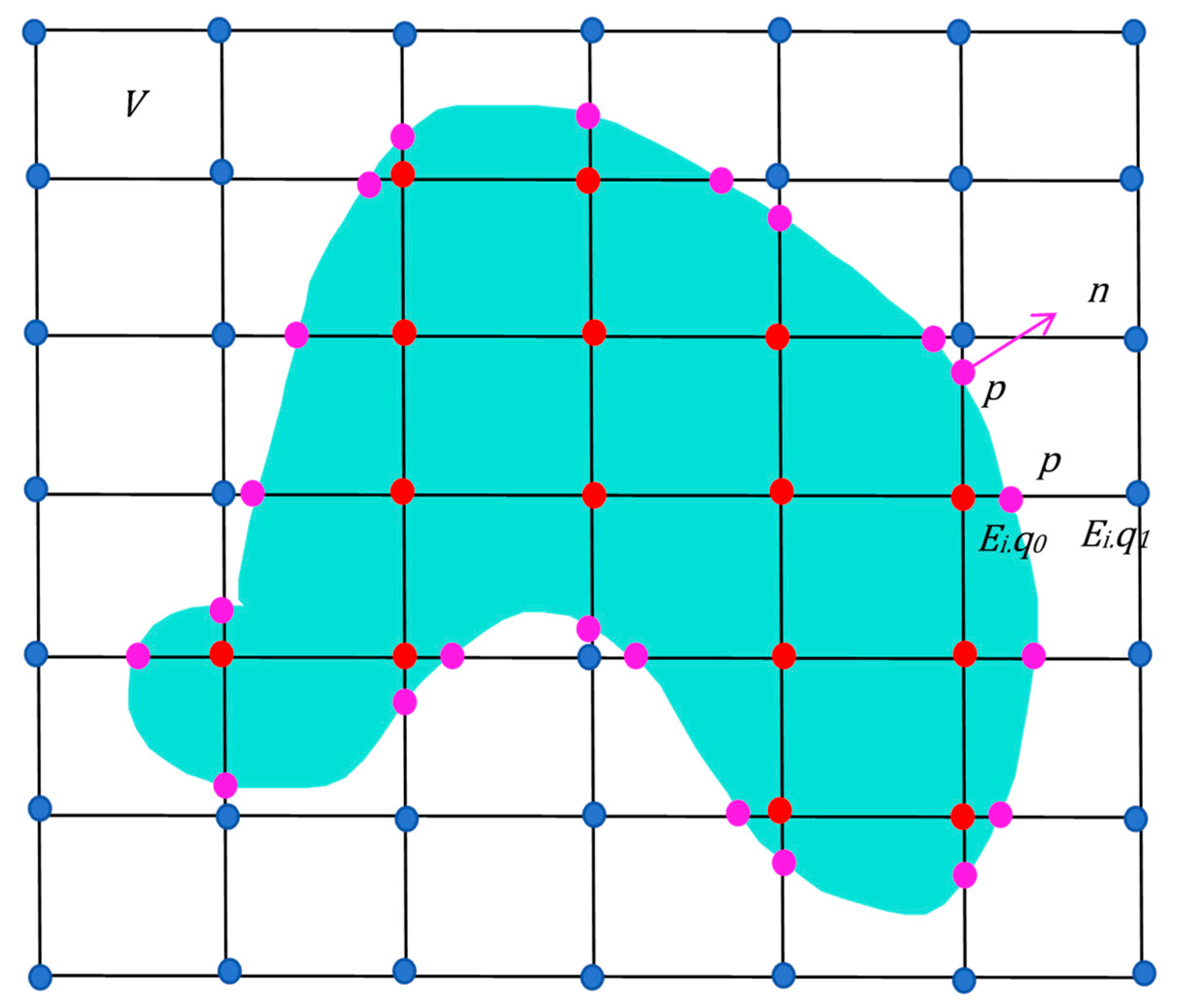
We use the Marching Cubes [23] algorithm to extract triangular patches, which can effectively generate the 3D mesh model from TSDF volume data. In the corresponding TSDF voxel data, we extract the triangular mesh corresponding to the zero isosurface. The endpoints of the corresponding triangular patches can be regarded as the intersection points of the sides of the cube in the voxel and the surface, which are generally obtained through linear interpolation, such as shown in Figure 5.
We notice that when the quality of the original depth map data is poor or the observation angle is insufficient, there are phenomena such as stripes and insufficient smoothness of the mesh surface. In order to overcome the reconstruction problem of such scenes, we further optimize the results extracted by Marching Cubes based on the facet assumption and smooth texture distribution constraints to obtain a smoother mesh model.
It is known that the point p i is the intersection point of the surface and an edge E i in the voxel cube, as shown in the pink point in Figure 4. The two endpoints in the corresponding voxel of the edge E i are E i . q 0 and E i . q 1 , such as the red point and the blue point. Among them, point q ∈ V, V is a voxel network, i.e., the square grid in the figure. For convenience, we only adjust the position of point p i on edge E i as follows:
p i = E i . q 0 + λ i E i . q 1 E i . q 0
Based on the above, we construct the energy term:
D p = i p t s d f E i . q 0 t s d f E i . q 1 × λ i t s d f E i . q 0 V u n i t 2 2
where tsdf (q) is the truncated signed distance corresponding to point q, and V u n i t is the side length of the smallest cube in voxel V.
Based on the small-plane assumption that points should be distributed near the plane corresponding to neighboring points, we construct the smoothing term as follows:
D s = i p j p a d j p i p j n j 2 2
where n i is the unit normal vector corresponding to p i , which can be obtained by interpolation.
Furthermore, we note that textures can also help us improve the quality of the mesh. That is, the direction of the gradient change in the voxel should be consistent with the brightness change between neighboring points. Therefore, we construct the following constraint term:
D r g b = i p j p a d j C p j + p i p j g j C p i 2 2
where g i is the texture gradient of point p i . C p i is the brightness of point p i , which can be expressed as follows:
C ( p i ) = E i . I 0 + λ i E i . I 1 E i . I 0
Meanwhile, we know that in the fused voxel, only the luminance change on the zero-equivalent plane is informative, i.e., the luminance transformation on the n i normal plane of the p i point. In the actual gradient calculation, it is necessary to project the luminance of the neighboring point q onto the normal plane. Let f(q) be the projection function corresponding to the point p i , then it can be calculated by the following equation:
f q = q n i q p i T n i
Similar to the method of Zhou [32], given C ( p i ) is the luminance of point p i , C p i u is the continuous luminance function of point p i , where u is the vector on the plane normal to point p i with p i as the origin, and there exists u n i = 0 . For the convenience of the computation, C p i u (u) is expanded as follows:
C p i u C p i + g i T n i
The texture gradient is obtained by solving the following equation by the least squares:
D g i = q A d j { p i } W q C p i f q p i C q 2
D g i q A d j { p i } W q C p i + g i T f q p C q 2  
where W q is the weight W q = V u n i t V u n i t + | n i ( q p i ) | . With the simultaneous attached constraint u n i = 0 , the texture gradient g i can be calculated.
Combine (18), (19) to obtain the following:
D r g b = i p j p a d j C p j + E i . q 0 + λ i E i . q 1 E i . q 0 p j g j E i . I 0 λ i E i . I 1 E i . I 0 2 2
D r g b = i p j p a d j C p j + E i . q 0 p j g j E i . I 0 λ i E i . I 1 E i . I 0 E i . q 1 E i . q 0 g j 2 2
It can be seen that D p , D s , and D r g b are all related to λ. Distribution iterative optimization is used, and the gradient and normal are updated each time to obtain better results.
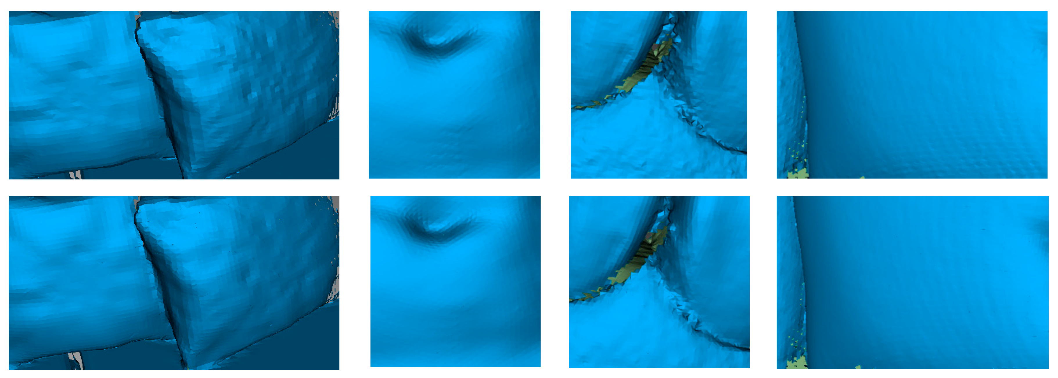
The following Figure 6 compares the performance of RGBTSDF direct mesh extraction and mesh extraction with texture constraints. It can be seen from the comparison that adding texture constraints can effectively remove noise and extract smoother and more natural meshes. Specifically, to more accurately reflect the meshes, flat shading is used for display.

4. Experiments and Results

To evaluate the performance and accuracy of the RGBTSDF system, two large RGB-D datasets are selected for experiments, and baseline tests are performed to test runtime performance, memory usage, and mapping accuracy. One is a public dataset of large scenes, and the other is a dataset collected using a commercial 3D scanner. For the public datasets, we choose TUM [33] and ICL-NUIM [34]. For the TUM dataset, we select the scene data “freiburg1_xyz”, and for the ICL-NUIM dataset, we select the trajectory “kt1” of “LivingRoom”. In addition, for different application scenarios, we also use two commercial 3D scanners to collect data, namely the Lynx 3D scanner independently developed by 3DMakerPro to collect the Venus model data and Furniture data. The above datasets verify application scenarios of different sizes, covering the collection range from 0.1 m to 5 m. Of course, the RGBTSDF system can map a larger scene range, and can achieve a wide range of scenes with a maximum length of 221.
The following comparisons are all performed under the same hardware configuration. The above datasets are tested for the time efficiency, space efficiency, and accuracy of RGBTSDF, the open-source algorithm library Open3D [35] (the version number is 0.14.1), the most popular VDBFusion [18], and the recent method Gradient-SDF [36]. The test hardware configurations are Intel Core i7-6700 eight-core (3.4 GHz), 32 GB RAM. All methods are evaluated using their C++ implementations, and all experiments are performed on a single-core CPU for comparison. Special note: in our open-source code RGBTSDF, three fusion methods are provided, namely TSDF, TinyTSDF, and ColorTSDF. TSDF and TinyTSDF do not have color information. TinyTSDF has been memory optimized. Details can be found in the open-source code. The following experiments use the TinyTSDF method.

4.1. Public Dataset

4.1.1. ICL-NUIM Dataset

The ICL-NUIM dataset is a synthetic RGB-D dataset. In order to be consistent with VDBFusion [18], we use the living room scene without simulated noise. The frame rate is 30 Hz, and the sensor resolution is 640 × 480. This dataset provides RGB-D images stored in PNG format along with ground truth camera poses, scanned at 965 frames. As shown in Table 1, on the ICL-NUIM dataset, our method is 1.5 times better in memory compared to VDBFusion, eight times better than Open3D, and tens of times better than Gradient-SDF. The efficiency is more than two times that of VDBFusion and Open3D, and more than ten times that of Gradient-SDF. Our method utilizes the sparse characteristics of volume, the grid octree data structure, and the hard coding data index so it can efficiently manage the scene and reduce memory consumption.
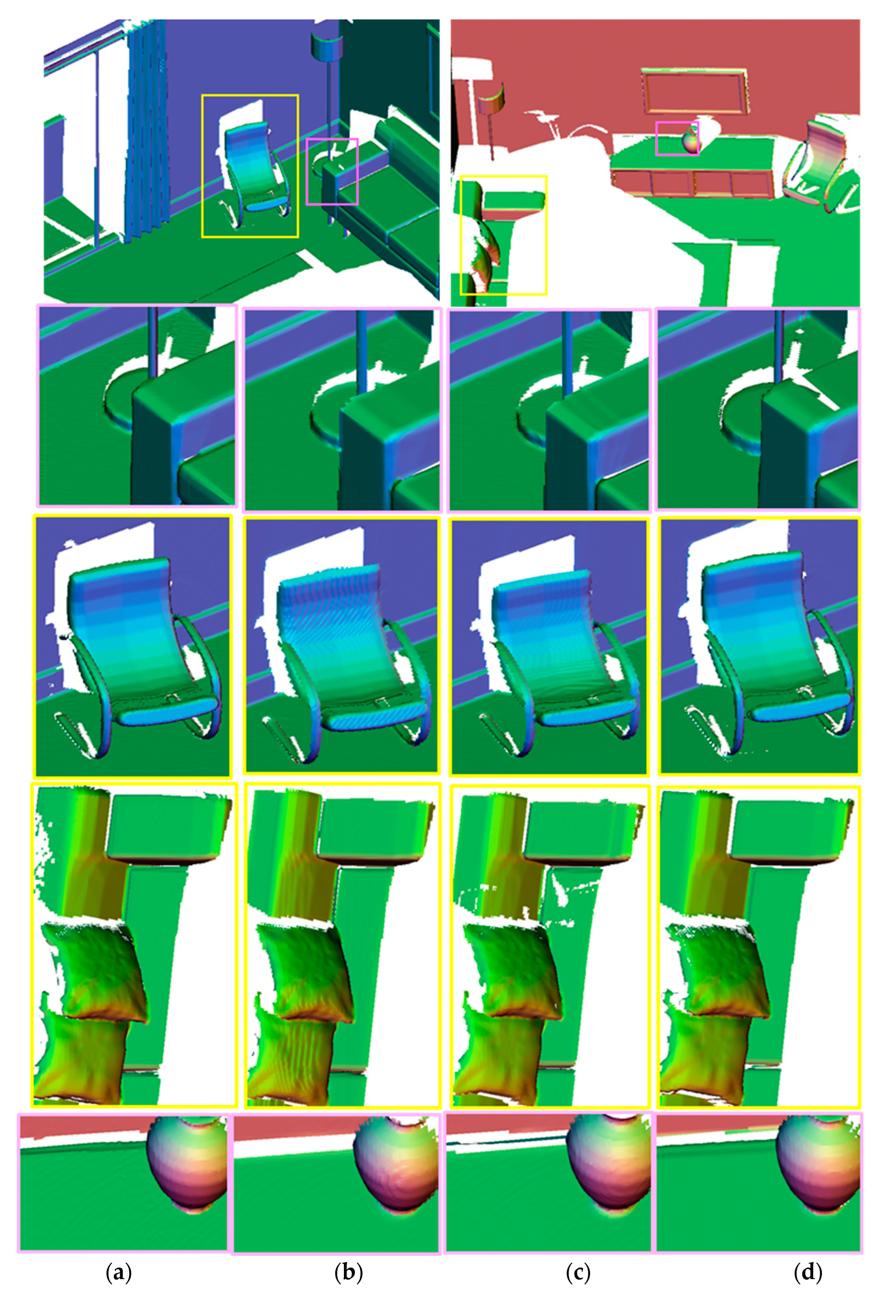
Figure 7 shows the fusion results and local details of the two scenes in the ICL-NUIM dataset. We find that the blocking effect of the VDBFusion method is obvious, while the mesh of Open3D and Gradient-SDF is not smooth enough. Our proposed RGBTSDF method fuses a smoother mesh by interpolating the depth map and optimizing the mesh based on texture constraints.

4.1.2. TUM Dataset

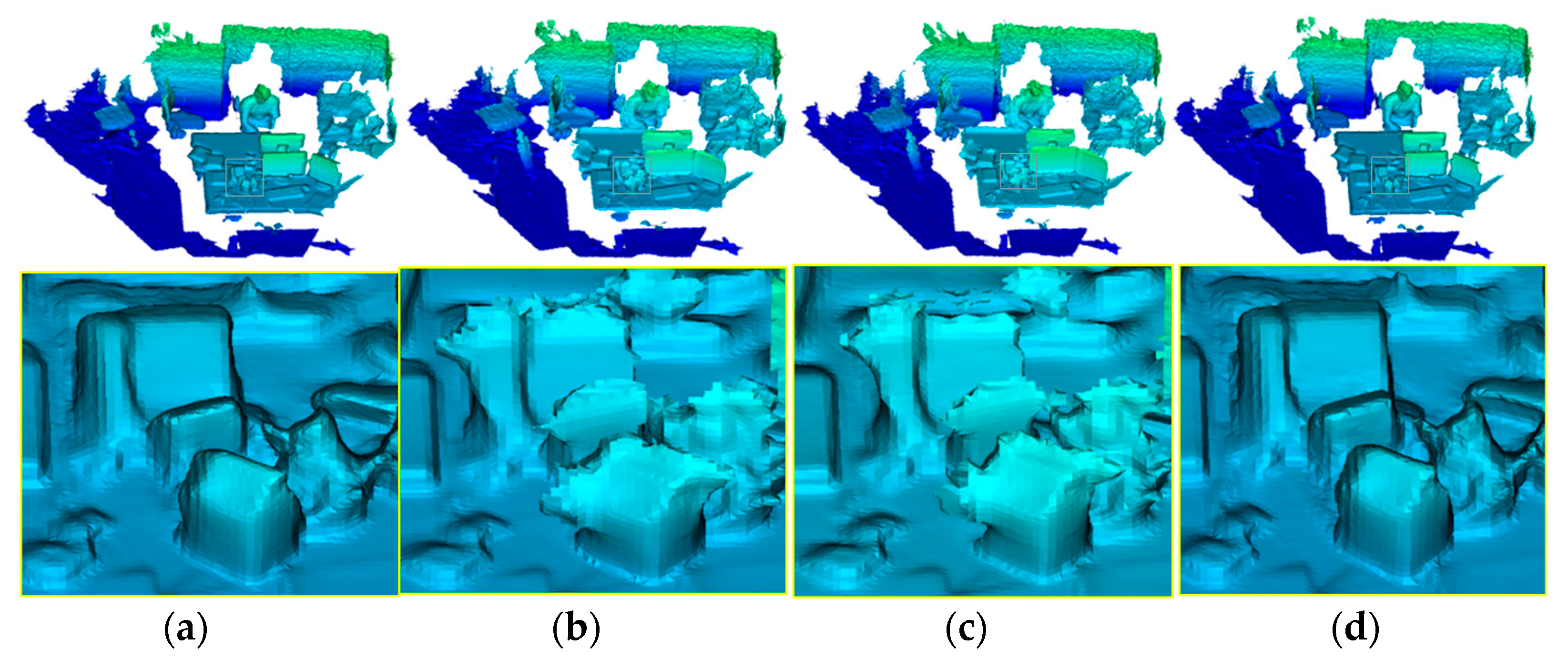
The TUM dataset is a large dataset containing both RGB-D data and ground truth data. In order to be consistent with VDBFusion, we use the freiburg1_xyz real office scene with a frame rate of 30 Hz and a resolution of 640 × 480. The dataset provides sequences of disordered RGB-D images stored in PNG format with 790 frames. RGB images need to be paired with depth maps according to the time and ground truth camera pose. Table 2 shows that our method improves memory by two times compared to VDBFusion, by 6.7 times compared to Open3D, and by ten times compared to Gradient-SDF. The efficiency is 5.6 times that of VDBFusion, 2.8 times that of Open3D, and more than ten times that of Gradient-SDF. Once again, the grid octree data structure proposed in the paper and the hard coded data indexing prove to be less memory-intensive and more efficient. Figure 8 shows the fusion results of different methods on the TUM dataset. It shows that our RGBTSDF method is smoother and less noisy than the other three methods and can effectively reconstruct three-dimensional indoor scenes.

4.2. Commercial 3D Scanner Data

4.2.1. Venus Model

The Venus model data were captured using 3DMakerPro’s proprietary Lynx 3D scanner. The acquisition frame rate is 10 Hz, the working distance is 400 mm to 900 mm, and the objects can be scanned from 100 mm to 2000 mm with a reconstruction accuracy of up to 0.1 mm. The sensor resolution is 640 × 512, and the data are provided with a depth map in PNG format and a color image in JPG format, as well as real camera poses with a frame rate of 849 frames. As can be seen in Table 3, for the Venus model data, our method has a memory improvement of two times over VDBFusion, 4.5 times over Open3D, and dozens of times over Gradient-SDF. The efficiency is also significantly improved compared to other methods.
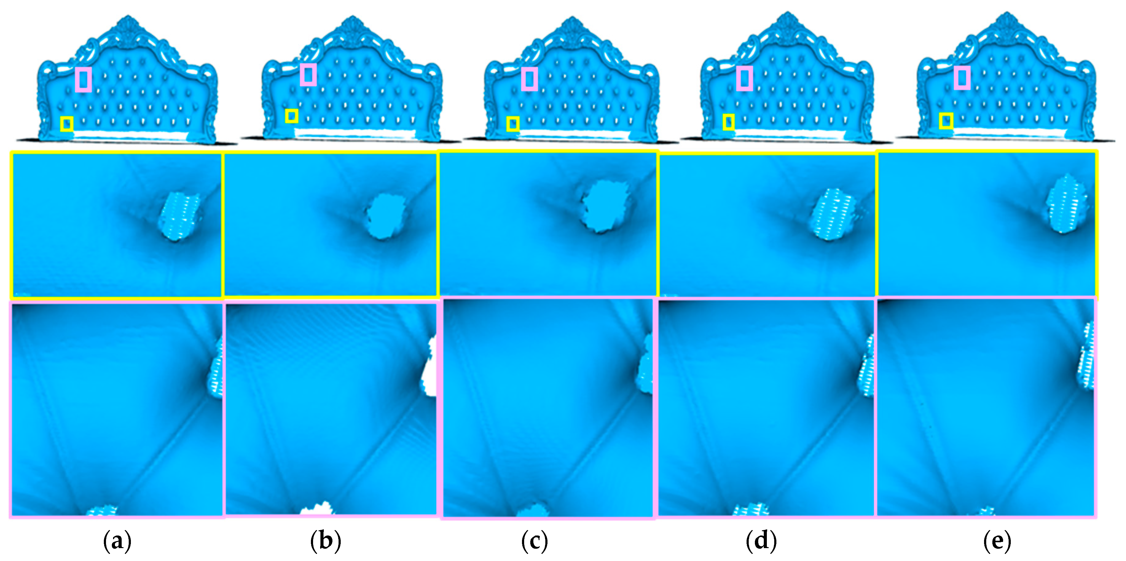
Figure 9 shows the fusion results and local details of different methods on the Venus model data, respectively. It shows that all methods obtain more complete modeling results, but the VDBFusion and Open3D methods have ripples, while our RGBTSDF method fuses a smoother mesh due to interpolation of the depth map and optimization of the mesh by combining the texture. Gradient-SDF has comparable reconstruction results to our method but is less efficient and more memory-intensive. In addition, when our method uses texture constraints, the results of mesh reconstruction are further improved to be smoother.

4.2.2. Furniture

Furniture is also collected through the Lynx 3D scanner independently developed by 3DMakerPro. The data provide a depth map stored in PNG format and a color image stored in JPG format, as well as the real camera pose with a frame number of 1023. As shown in Table 4 and Figure 10, we can see the fusion results of the four methods on the Furniture. Among them, the VDBFusion method has obvious ripple phenomenon. The RGBTSDF, Open3D, and Gradient-SDF have achieved reasonable fusion results, but in comparison, our method is faster and saves memory.

4.3. Surface Reconstruction Quality Evaluation and Analysis

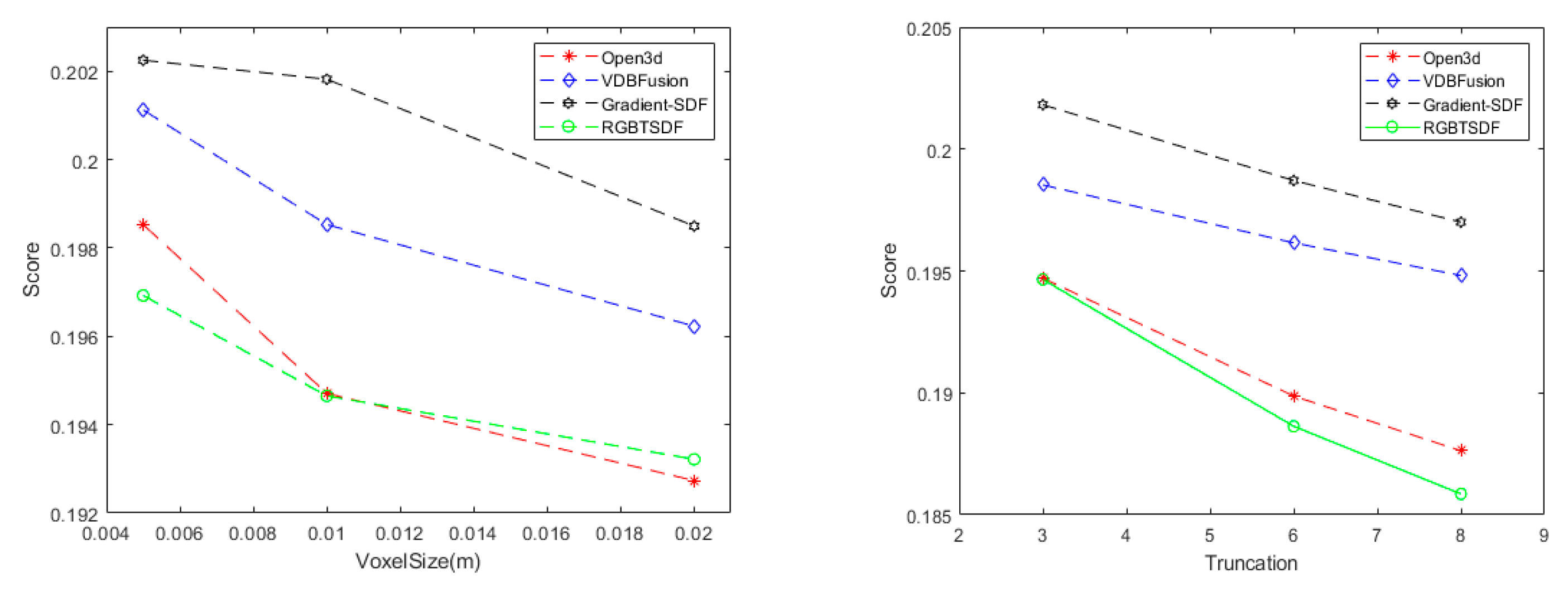
Since ground truth is available in the ICL-NUIM dataset, this dataset is chosen in this subsection to test the accuracy of the mesh reconstructed by the mentioned fusion methods. For accuracy evaluation, we use the SurfReg tool (“GitHub-mp3guy/SurfReg: Automatic surface registration tool for ICL-NUIM datasets”), which aligns and outputs scores to evaluate the reconstructed model. The effect of different voxel sizes and truncation on the reconstruction is discussed here, and the reconstructions produced by Open3D, VDBFusion, Gradient-SDF, and RGBTSDF fusion methods are quantitatively analyzed with the real 3D surface model of the ground, as shown in Figure 11.
On the left are the score curves of the ground truth model evaluated by SurfReg with the reconstructed model generated by the Open3D, VDBFusion, Gradient-SDF, and RGBTSDF fusion methods when truncation is set to 3 and the voxel size is 0.005 m, 0.01 m, and 0.02 m, respectively. Smaller values indicate greater closeness to the true value. It shows that the smaller the voxel size for all methods, the higher the accuracy of the reconstruction, but the memory consumption also increases. Our method achieves the highest reconstruction accuracy at a voxel size of 0.005 m, which is comparable to Open3D’s accuracy as the voxel size gets smaller, but our method is faster and uses less memory.
The right figure shows the model accuracy scores produced by the Open3D, VDBFusion, Gradient-SDF, and RGBTSDF fusion methods when the voxel size is set to 0.01 m and the truncation is set to 3, 6, and 8, respectively. It can be seen from the figure that the larger the truncation, the higher the scores of all the reconstruction methods. Our method achieves excellent reconstruction results at different settings.

4.4. Discussion

The above experimental results show that the RGBTSDF method proposed in this paper performs well on different datasets in terms of memory consumption, mapping time, fusion effect, etc. The grid octree method used in RGBTSDF can manage and expand the data more simply and efficiently than the VoxelHashing method in Open3D. Meanwhile, the hard coding method in RGBTSDF can insert, update, and index the data faster than the hash table method in VDBFusion. In addition, comparing the final fusion effect, it is found that the meshes of VDBFusion and Open3D have blocky and wavy phenomena and are easily affected by noise, while RGBTSDF interpolates the depth and obtains a more accurate surface depth value, which effectively overcomes the blocky effect due to quantization error and fuses the meshes more smoothly. At the same time, RGBTSDF adds a texture constraint optimization enhancement to the Marching Cubes algorithm, which further improves the quality of the mesh.
However, the current RGBTSDF is mainly applicable to the fusion of rigid objects and has not considered the reconstruction of dynamic scenes. In later research, we will focus on the fusion of non-rigid scenes as well as dynamic fusion to represent the dynamic scene motion by describing the parameterization of the dense volumetric torsion field to achieve non-rigid real-time reconstruction. In addition, although the CPU version of RGBTSDF can already achieve real-time performance, we will subsequently consider its subsequent deployment on GPU to further improve the reconstruction efficiency.

5. Conclusions

In this paper, we propose a volume mapping method, RGBTSDF, based on TSDF representation. The method designs a special octree data structure called grid octree and incorporates a hard coding approach for data indexing to achieve efficient, low-memory data management for large scenes. Meanwhile, the mapping accuracy is improved by deep interpolation and grid optimization. Our mapping framework is simple and efficient for scene reconstruction of different sizes and resolutions and can be quickly integrated with RGB-D data acquired from different 3D sensors.
Experiments on public and commercial datasets show that the RGBTSDF system is faster and uses less memory than other open-source mapping frameworks. Evaluation of mapping accuracy shows that our approach provides higher quality mappings. Finally, we open-source our code with C++ and Python interfaces, and we also provide datasets collected by commercial 3D scanners to facilitate comparative experiments. We hope that the open-source library will facilitate further research and provide a basic mapping framework for real-time tracking, optimization, and related AI applications. The code and data can be available at https://github.com/walkfish8/rgbtsdf (accessed on 26 August 2024).

Author Contributions

Conceptualization, Y.L.; Data curation, X.Z.; Funding acquisition, Q.H.; Investigation, Y.C.; Methodology, Y.L. and S.H.; Resources, Y.D. and X.Z.; Software, S.H.; Supervision, Q.H.; Visualization, P.Z.; Writing—original draft, Y.L. and S.H. All authors have read and agreed to the published version of the manuscript.

Funding

This study was supported by the State Key Laboratory of Geo-Information Engineering (SKLGIE2023-M-2-1); Wuhan Ruler Technology Foundation (2023KJB203); and National Natural Science Foundation of China (42371439).

Data Availability Statement

The ICL-NUIM dataset and TUM dataset can be obtained by applying for them at http://www.doc.ic.ac.uk/~ahanda/VaFRIC/iclnuim.html, accessed on 1 May 2024 and https://cvg.cit.tum.de/data/datasets/rgbd-dataset, accessed on 1 May 2024, and our scanner dataset is available on request from the author.

Conflicts of Interest

The authors declare that this study received funding from Wuhan Ruler Technology. The funder was not involved in the study design, collection, analysis, interpretation of data, the writing of this article or the decision to submit it for publication.

References

  1. Izadi, S.; Kim, D.; Hilliges, O.; Molyneaux, D.; Newcombe, R.; Kohli, P.; Shotton, J.; Hodges, S.; Freeman, D.; Davison, A. Kinectfusion: Real-Time 3D Reconstruction and Interaction Using a Moving Depth Camera. In Proceedings of the 24th Annual ACM Symposium on User Interface Software and Technology, Santa Barbara, CA, USA, 16–19 October 2011; pp. 559–568. [Google Scholar]
  2. Curless, B.; Levoy, M. A Volumetric Method for Building Complex Models from Range Images. In Proceedings of the 23rd Annual Conference on Computer Graphics and Interactive Techniques, New Orleans, LA, USA, 4–9 August 1996; pp. 303–312. [Google Scholar]
  3. Cao, Y.; Liu, Z.; Kuang, Z.; Kobbelt, L.; Hu, S. Learning to Reconstruct High-Quality 3D Shapes with Cascaded Fully Convolutional Networks. In Proceedings of the European Conference on Computer Vision (ECCV), Munich, Germany, 8–14 September 2018; pp. 616–633. [Google Scholar]
  4. Isler, S.; Sabzevari, R.; Delmerico, J.; Scaramuzza, D. An Information Gain Formulation for Active Volumetric 3D Reconstruction. In Proceedings of the 2016 IEEE International Conference on Robotics and Automation (ICRA), Stockholm, Sweden, 16–21 May 2016; pp. 3477–3484. [Google Scholar]
  5. Hinzmann, T.; Schönberger, J.L.; Pollefeys, M.; In Siegwart, R. Mapping on the Fly: Real-Time 3D Dense Reconstruction, Digital Surface Map and Incremental Orthomosaic Generation for Unmanned Aerial Vehicles. In Proceedings of the Field and Service Robotics: Results of the 11th International Conference, Zurich, Switzerland, 12–15 September 2017; Springer: Berlin/Heidelberg, Germany, 2018; pp. 383–396. [Google Scholar]
  6. Li, S.; Cheng, M.; Liu, Y.; Lu, S.; Wang, Y.; Prisacariu, V.A. Structured Skip List: A Compact Data Structure for 3D Reconstruction. In Proceedings of the 2018 IEEE/RSJ International Conference on Intelligent Robots and Systems (IROS), Madrid, Spain, 1–5 October 2018; pp. 1–7. [Google Scholar]
  7. Slavcheva, M.; Kehl, W.; Navab, N.; Ilic, S. SDF-2-SDF registration for real-time 3D reconstruction from RGB-D data. Int. J. Comput. Vision 2018, 126, 615–636. [Google Scholar] [CrossRef]
  8. Zheng, Z.; Yu, T.; Li, H.; Guo, K.; Dai, Q.; Fang, L.; Liu, Y. Hybridfusion: Real-Time Performance Capture Using a Single Depth Sensor and Sparse Imus. In Proceedings of the European Conference on Computer Vision (ECCV), Tel Aviv, Israel, 23–27 October 2018; pp. 384–400. [Google Scholar]
  9. Hornung, A.; Wurm, K.M.; Bennewitz, M.; Stachniss, C.; Burgard, W. OctoMap: An efficient probabilistic 3D mapping framework based on octrees. Auton. Robot. 2013, 34, 189–206. [Google Scholar] [CrossRef]
  10. Nießner, M.; Zollhöfer, M.; Izadi, S.; Stamminger, M. Real-time 3D reconstruction at scale using voxel hashing. ACM Trans. Graph. 2013, 32, 1–11. [Google Scholar] [CrossRef]
  11. Bylow, E.; Sturm, J.; Kerl, C.; Kahl, F.; Cremers, D. Real-Time Camera Tracking and 3D Reconstruction Using Signed Distance Functions. In Proceedings of the Robotics: Science and Systems (RSS) Conference 2013, Berlin, Germany, 24–28 June 2013. [Google Scholar]
  12. Newcombe, R.A.; Izadi, S.; Hilliges, O.; Molyneaux, D.; Kim, D.; Davison, A.J.; Kohi, P.; Shotton, J.; Hodges, S.; Fitzgibbon, A. Kinectfusion: Real-Time Dense Surface Mapping and Tracking. In Proceedings of the 2011 10th IEEE international Symposium on Mixed and Augmented Reality, Basel, Switzerland, 26–29 October 2011; pp. 127–136. [Google Scholar]
  13. Steinbrücker, F.; Sturm, J.; Cremers, D. Volumetric 3D Mapping in Real-Time on a CPU. In Proceedings of the 2014 IEEE International Conference on Robotics and Automation (ICRA), Hong Kong, China, 7 May–31 June 2014; pp. 2021–2028. [Google Scholar]
  14. Chen, J.; Bautembach, D.; Izadi, S. Scalable real-time volumetric surface reconstruction. ACM Trans. Graph. 2013, 32, 111–113. [Google Scholar] [CrossRef]
  15. Kähler, O.; Prisacariu, V.; Valentin, J.; Murray, D. Hierarchical voxel block hashing for efficient integration of depth images. IEEE Robot. Autom. Lett. 2015, 1, 192–197. [Google Scholar] [CrossRef]
  16. Fuhrmann, S.; Goesele, M. Fusion of depth maps with multiple scales. ACM Trans. Graph. 2011, 30, 1–8. [Google Scholar] [CrossRef]
  17. Dryanovski, I.; Klingensmith, M.; Srinivasa, S.S.; Xiao, J. Large-scale, real-time 3D scene reconstruction on a mobile device. Auton. Robot. 2017, 41, 1423–1445. [Google Scholar] [CrossRef]
  18. Vizzo, I.; Guadagnino, T.; Behley, J.; Stachniss, C. Vdbfusion: Flexible and efficient tsdf integration of range sensor data. Sensors 2022, 22, 1296. [Google Scholar] [CrossRef] [PubMed]
  19. Museth, K. VDB: High-resolution sparse volumes with dynamic topology. ACM Trans. Graph. 2013, 32, 1–22. [Google Scholar] [CrossRef]
  20. Oleynikova, H.; Taylor, Z.; Fehr, M.; Siegwart, R.; Nieto, J. Voxblox: Incremental 3d Euclidean Signed Distance Fields for On-Board Mav Planning. In Proceedings of the 2017 IEEE/RSJ International Conference on Intelligent Robots and Systems (IROS), Vancouver, BC, Canada, 24–28 September 2017; pp. 1366–1373. [Google Scholar]
  21. Vizzo, I.; Chen, X.; Chebrolu, N.; Behley, J.; Stachniss, C. Poisson Surface Reconstruction for LiDAR Odometry and Mapping. In Proceedings of the 2021 IEEE International Conference on Robotics and Automation (ICRA), Xi’an, China, 30 May–5 June 2021; pp. 5624–5630. [Google Scholar]
  22. Kazhdan, M.; Hoppe, H. Screened poisson surface reconstruction. ACM Trans. Graph. 2013, 32, 1–13. [Google Scholar] [CrossRef]
  23. Lorensen, W.E.; Cline, H.E. Marching cubes: A high resolution 3D surface construction algorithm. In Seminal Graphics: Pioneering Efforts that Shaped the Field; Association for Computing Machinery: New York, NY, USA, 1998; pp. 347–353. [Google Scholar]
  24. Dong, W.; Park, J.; Yang, Y.; Kaess, M. GPU Accelerated Robust Scene Reconstruction. In Proceedings of the 2019 IEEE/RSJ International Conference on Intelligent Robots and Systems (IROS), Macau, China, 3–8 November 2019; pp. 7863–7870. [Google Scholar]
  25. Dong, W.; Shi, J.; Tang, W.; Wang, X.; Zha, H. An Efficient Volumetric Mesh Representation for Real-Time Scene Reconstruction Using Spatial Hashing. In Proceedings of the 2018 IEEE International Conference on Robotics and Automation (ICRA), Brisbane, QLD, Australia, 21–26 May 2018; pp. 6323–6330. [Google Scholar]
  26. Hilton, A.; Stoddart, A.J.; Illingworth, J.; Windeatt, T. Marching Triangles: Range Image Fusion for Complex Object Modelling. In Proceedings of the 3rd IEEE International Conference on Image Processing, Lausanne, Switzerland, 19 September 1996; pp. 381–384. [Google Scholar]
  27. Sharf, A.; Lewiner, T.; Shklarski, G.; Toledo, S.; Cohen-Or, D. Interactive topology-aware surface reconstruction. ACM Trans. Graph. 2007, 26, 43. [Google Scholar] [CrossRef]
  28. Premebida, C.; Garrote, L.; Asvadi, A.; Ribeiro, A.P.; Nunes, U. High-Resolution Lidar-Based Depth Mapping Using Bilateral Filter. In Proceedings of the 2016 IEEE 19th International Conference on Intelligent Transportation Systems (ITSC), Rio de Janeiro, Brazil, 1–4 November 2016; pp. 2469–2474. [Google Scholar]
  29. Wu, C.; Zollhöfer, M.; Nießner, M.; Stamminger, M.; Izadi, S.; Theobalt, C. Real-time shading-based refinement for consumer depth cameras. ACM Trans. Graph. 2014, 33, 1–10. [Google Scholar] [CrossRef]
  30. Xie, W.; Wang, M.; Qi, X.; Zhang, L. 3D Surface Detail Enhancement from a Single Normal Map. In Proceedings of the IEEE International Conference on Computer Vision, Venice, Italy, 22–29 October 2017; pp. 2325–2333. [Google Scholar]
  31. Zhou, Q.; Neumann, U. 2.5D Dual Contouring: A Robust Approach to Creating Building Models from Aerial Lidar Point Clouds. In Proceedings of the Computer Vision—ECCV 2010: 11th European Conference on Computer Vision, Heraklion, Crete, Greece, 5–11 September 2010; Proceedings, Part III 11. Springer: Berlin/Heidelberg, Germany, 2010; pp. 115–128. [Google Scholar]
  32. Park, J.; Zhou, Q.; Koltun, V. Colored point cloud registration revisited. In Proceedings of the 2017 IEEE International Conference on Computer Vision (ICCV), Venice, Italy, 24–27 October 2017; pp. 143–152. [Google Scholar]
  33. Sturm, J.; Engelhard, N.; Endres, F.; Burgard, W.; Cremers, D. A Benchmark for the Evaluation of RGB-D SLAM Systems. In Proceedings of the IEEE/RSJ International Conference on Intelligent Robots and Systems, Vilamoura-Algarve, Portuga, l7–12 October 2012; pp. 573–580. [Google Scholar]
  34. Handa, A.; Whelan, T.; McDonald, J.; Davison, A.J. A Benchmark for RGB-D Visual Odometry, 3D Reconstruction and SLAM. In Proceedings of the 2014 IEEE International Conference on Robotics and Automation (ICRA), Hong Kong, China, 31 May–7 June 2014; pp. 1524–1531. [Google Scholar]
  35. Zhou, Q.; Park, J.; Koltun, V. Open3D: A modern library for 3D data processing. arxiv 2018, arXiv:1801.09847. [Google Scholar]
  36. Sommer, C.; Sang, L.; Schubert, D.; Cremers, D. Gradient-sdf: A Semi-Implicit Surface Representation for 3D Reconstruction. In Proceedings of the 2022 IEEE/CVF Conference on Computer Vision and Pattern Recognition (CVPR), New Orleans, LA, USA, 18–24 June 2022; pp. 6280–6289. [Google Scholar]
Figure 1. The pipeline of RGBTSDF.
Remotesensing 16 03188 g001
Figure 2. The structure of an octree.
Remotesensing 16 03188 g002
Figure 3. The structure of a grid octree.
Remotesensing 16 03188 g003
Figure 4. The diagram of hard coding.
Remotesensing 16 03188 g004
Figure 5. 2D schematic of Marching Cubes.
Remotesensing 16 03188 g005
Figure 6. From top to bottom, the first row depicts the results of direct mesh extraction, while the second row shows the effects of mesh extraction with texture constraints applied.
Remotesensing 16 03188 g006
Figure 7. Qualitative and detail results of different methods on the ICL-NUIM dataset. (a) Open3D; (b) VDBFusion; (c) Gradient-SDF; (d) RGBTSDF.
Remotesensing 16 03188 g007
Figure 8. Qualitative results of different methods on the TUM dataset. (a) Open3D; (b) VDBFusion; (c) Gradient-SDF; (d) RGBTSDF.
Remotesensing 16 03188 g008
Figure 9. Qualitative and details results of different methods on the Venus model data. (a) Open3D; (b) VDBFusion; (c) Gradient-SDF (d) RGBTSDF; (e) RGBTSDF of mesh extraction with texture constraints.
Remotesensing 16 03188 g009
Figure 10. Qualitative and details results of different methods on the Furniture. (a) Open3D; (b) VDBFusion; (c) Gradient-SDF (d) RGBTSDF; (e) RGBTSDF of mesh extraction with texture constraints.
Remotesensing 16 03188 g010
Figure 11. Comparison of reconstruction scores for four fusion methods with different voxel sizes and truncation.
Remotesensing 16 03188 g011
Table 1. Quantitative results of different methods on the ICL-NUIM dataset.
ICL-NUIMVoxel Size (0.01 m)Truncation (3 Voxels)
Frame RateMemory SizeDisk Size
Open3D4.61329.7 MB35.10 MB
VDBFusion4.6364 MB34.39 MB
Gradient-SDF1.211293.2 MB25.94 MB
RGBTSDF11.5641.2 MB34.75 MB
Table 2. Quantitative results of different methods on the TUM dataset.
TUMVoxel Size (0.01 m)Truncation (8 Voxels)
Frame RateMemory SizeDisk Size
Open3D5.28201.5 MB12.85 MB
VDBFusion2.6962.4 MB13.81 MB
Gradient-SDF1.02766.1 MB11.65 MB
RGBTSDF15.2229.9 MB12.74 MB
Table 3. Quantitative results of different methods on the Venus model data.
Venus ModelVoxel Size (0.002 m)Truncation (3 Voxels)
Frame RateMemory SizeDisk Size
Open3D2.151457.2 MB23.07 MB
VDBFusion7.03697.3 MB23.38 MB
Gradient-SDF3.06660.4 MB21.84 MB
RGBTSDF19.72325 MB23.84 MB
Table 4. Quantitative results of different methods on the Furniture.
Ornament of Guan GongVoxel Size (0.001 m)Truncation (3 Voxels)
Frame RateMemory SizeDisk Size
Open3D1.452959 MB59.68 MB
VDBFusion7.27931.6 MB59.60 MB
Gradient-SDF2.821367.6 MB57.26 MB
RGBTSDF18.05443.7 MB60.40 MB
Disclaimer/Publisher’s Note: The statements, opinions and data contained in all publications are solely those of the individual author(s) and contributor(s) and not of MDPI and/or the editor(s). MDPI and/or the editor(s) disclaim responsibility for any injury to people or property resulting from any ideas, methods, instructions or products referred to in the content.