Harbor Detection in Polarimetric SAR Images Based on Context Features and Reflection Symmetry

Abstract

The detection of harbors presents difficulties related to their diverse sizes, varying morphology and scattering, and complex backgrounds. To avoid the extraction of unstable geometric features, in this paper, we propose an unsupervised harbor detection method for polarimetric SAR images using context features and polarimetric reflection symmetry. First, the image is segmented into three region types, i.e., water low-scattering regions, strong-scattering urban regions, and other regions, based on a multi-region Markov random field (MRF) segmentation method. Second, by leveraging the fact that harbors are surrounded by water on one side and a large number of buildings on the other, the coastal narrow-band area is extracted from the low-scattering regions, and the harbor regions of interest (ROIs) are determined by extracting the strong-scattering regions from the narrow-band area. Finally, by using the scattering reflection asymmetry of harbor buildings, harbors are identified based on the global threshold segmentation of the horizontal, vertical, and circular co- and cross-polarization correlation powers of the extracted ROIs. The effectiveness of the proposed method was validated with experiments on RADARSAT-2 quad-polarization images of Zhanjiang, Fuzhou, Lingshui, and Dalian, China; San Francisco, USA; and Singapore. The proposed method had high detection rates and low false detection rates in the complex coastal environment scenarios studied, far outperforming the traditional spatial harbor detection method considered for comparison.

1. Introduction

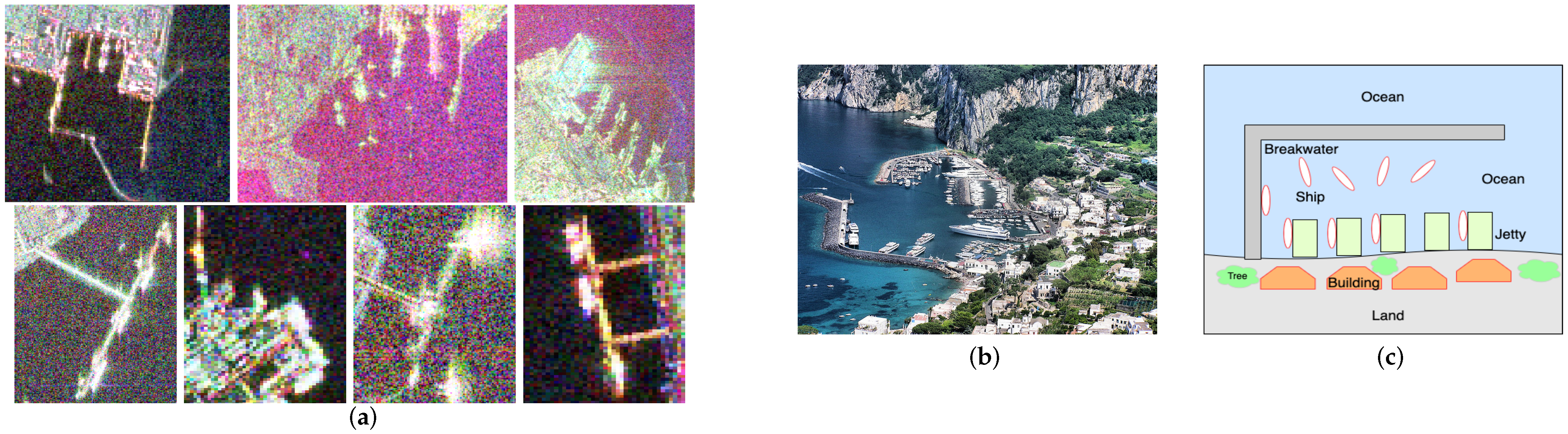
Harbors are transport hubs located along the coastline or on river banks with facilities correlated to land and water transport for ships to berth, find shelter, and collect and distribute cargo [1,2]. The automatic detection of artificial harbors in synthetic aperture radar (SAR) images is important for harbor monitoring, automatic navigation, image alignment, ground observation in coastal zones, and harbor area ship detection. Depending on the function, use, and scale, harbors can be large, medium, and small and can be classified as either natural or artificial and as open, closed, or mixed harbors. Due to the variability in coastal topography and tides in different regions, the size, morphological structure, and composition of different harbors in complex scenes are very different, and so is the scattering intensity distribution of harbor land cover and background areas, as shown in Figure 1a. These feature differences increase the difficulty of harbor detection in SAR images.

As shown in Figure 1b, harbors located on the coastline are composed of several components, including harbor jetties, breakwaters, other buildings in the harbor, moored vessels, and other land areas in the harbor and harbor waters. Figure 1c shows the diagram structure of a harbor. In terms of geometric characteristics, jetties and breakwaters are often long and narrow, are linear or present little curvature, and form concave–convex and orderly folding lines between each other, which makes the harbor contour geometrically distinct compared with the natural terrain of the coast. In terms of scattering characteristics, due to the large number of corner reflector structures (e.g., harbor warehouses, administrative facilities, and containers) in the harbor land area, the latter tends to have stronger backscattering than the surrounding land areas. Moreover, the quays in the harbor also show stronger backscattering because of the internal metal structure and the moored ships. In polarimetric SAR images, harbor buildings and waters also show significant polarimetric characteristics. In harbors built with reinforced concrete, the strong single scattering from isolated metals and the strong dihedral scattering between buildings, between buildings and the ground, and between buildings and the water surface make the polarimetric scattering in the harbor area very complex. The strong second echo sidelobe jamming from harbor buildings results in scattering with high intensity and complex composition in the harbor waters compared with the surrounding waters. In addition to the geometric and scattering characteristics, the surrounding land cover of the harbor area can provide contextual features for harbor detection and identification; for example, docked ships show high scattering intensity and significant polarization features.

Depending on the harbor characteristics, harbor detection methods can be classified into three categories: geometric feature methods, scattering feature methods, and deep learning methods. In the former, detection is performed by extracting geometric structural features unique to the harbor area. Since harbors are located on the sea–land boundary, the accurate segmentation of the latter is a prerequisite for geometric feature extraction. Many research works on sea–land segmentation and coastline detection have been recently conducted, and the methods used included edge detection [3], watershed transformation [4], Markov random field (MRF) segmentation [5], and level-set segmentation [6,7,8]. Based on accurate sea–land segmentation and coastline detection, the points, lines, and structures of the harbor contour can be extracted for harbor detection. Based on the difference in the density of harbor and non-harbor contour feature points, Liu et al. [9] developed a harbor detection method using coastline feature point merging. Based on the parallel contour lines on both sides of harbor jetties and breakwaters, Liu et al. [10] established a harbor detection method using parallel curve features. By leveraging the feature of the concave convex orderliness of jetty contours, Li et al. [11] proposed the use of the wavelet transform for extracting the contour line corner points and subsequently performing harbor detection by measuring corner-point chain code descriptors. The authors of [12] developed a method using edge detection combined with scale rotation-invariant key point detection for contour feature extraction. Schwan et al. [13] established a blackboard-based production system (BPS) for the step-by-step generation of the lines, long lines, folds, U-shaped structures, and E-shaped structures of harbor scenes. By leveraging the strong closure characteristic of harbor contours, Zhang et al. [14] developed a method for the detection of the latter based on measuring the shoreline contour closure. Based on the fact that harbor jetties and breakwaters protrude from the water, Liu et al. [15] developed a multi-directional jetty scanning harbor detection method. However, due to the strong, coherent speckle noise of SAR images, the complexity of the distribution of coastal land cover, and the variety of harbor morphology, the extraction of geometric features such as corner points and straight lines is cumbersome and does not provide accurate results, and features such as parallelism, folding lines, and closeness cannot be accurately measured. Particularly in large harbors, where the water side is subject to noise derived from the sidelobe echo of strong scatterers, the detection of the coastline along the harbor presents bias, resulting in incorrect geometric feature extraction.

Detection approaches using scattering features are based on either the modeling of the statistical distribution of the harbor land cover scattering intensity or coherency matrix or on the construction of a scattering model used to decompose such scattering or coherency matrix. In terms of statistical modeling, for a homogeneous region in a harbor area, the scattering intensity of the single polarization channel of a SAR image obeys the gamma distribution, and the scattering coherency or covariance matrix of the polarimetric SAR image approximately obeys the complex Wishart distribution [16]. For heterogeneous regions, assuming that the texture distribution is a gamma distribution, the scattering intensity and coherency matrix of the land cover approximately obey the K-distribution [17]. A more accurate statistical model of harbor land cover can be obtained by modeling more complex texture distributions, such as the KummerU distribution model of the polarimetric coherency matrix obtained by Bombrun et al. [18] using Fisher’s distribution to describe the texture distribution. Based on accurate statistical modeling, different harbor land cover types, including harbor waters, soil, buildings, and vegetation, can be extracted by using thresholding [19], region merging [20], MRF segmentation [5,21], the graph cut method [22], level-set segmentation [23,24], etc. However, due to the complexity of harbor area land cover and the mutual interference of scattering from adjacent buildings, it is difficult to employ the existing statistical distribution models for accurately describing land cover in harbor areas.

In terms of scattering modeling, the scattering components of harbor areas are complex due to the double and multiple scattering between the different harbor buildings and land cover types in polarimetric SAR images. The buildings in harbor areas can be detected by extracting polarimetric parameters and using different polarimetric decomposition methods. Cloude et al. [25] developed a method for decomposing the eigenvalues of the coherent scattering matrix of the target to define the parameters of polarization entropy and scattering angle characterizing the degree of scattering randomness of the target; the land cover types can then be classified into several categories according to the range of values of polarization entropy and scattering angle. In their study, the scattering components of buildings were located in the medium–high-entropy and high-scattering-angle regions. Compared with the backscattering of natural land cover, that of buildings is asymmetric, and this difference is directly reflected in the correlation coefficients of the co- and cross-polarization components of the target. Moriyama et al. [26] developed a building extraction method based on the polarization correlation coefficients, and Wang et al. [27] established a method using the reflection symmetry parameter for extraction. Based on the fact that the correlation coefficients of the co- and cross-polarization components of an asymmetric target are equally significant on a circularly polarized orthogonal basis when changing polarization bases, Ainsworth et al. [28] defined a circular polarization correlation coefficient for the extraction of buildings. Based on the fact that the orientation angle, which is directly related to the polarization correlation coefficient, can also be used to discriminate asymmetric targets, Kajimoto et al. [29] developed a building classification method using the polarization orientation angle. Based on the extracted harbor buildings, Liu et al. [15] established a harbor detection method using jetty scanning and building extraction, with which it is possible to detect candidate harbor areas by performing multi-directional jetty scanning and identify harbors by evaluating the percentage of strong-scattering buildings in the region of interest (ROI). Liu et al. [1] developed a port detection method based on port water and building extraction where the volume scattering power obtained by a modified three-component decomposition is used for water–land separation, and a double-scattering power–volume scattering power ratio parameter was established for the harbor–water and non-harbor–water separation. However, due to the complexity and irregularity of buildings in harbor areas, the analysis of the scattering components of harbor building and water areas is very complex, and so is extracting scattering components specific to harbor land cover.

In harbor detection methods based on deep learning, the harbor model is built based on learning from a large number of harbor images with different morphology, avoiding manually designed feature extraction. Ye et al. [30] developed a harbor detection method based on deep residual networks and single-step neural networks, in which ResNet [31] is first used to extract the coastal zone regions, and then SSD networks are used to identify harbors in coastal zone regions. Wang et al. [32,33] established a harbor detection method combining geometric features and deep learning, in which multi-directional jetty scanning is first performed to extract the harbor ROIs, and then a multi-layer neural network is built to classify them. However, deep learning relies on a large number of samples for training, and in practice, it is difficult to cover harbor regions with varying morphology, size, and scattering type.

In summary, it is difficult to employ the existing detection methods for detecting harbors accurately and robustly due to the strong coherent speckle noise in SAR images, strong-scatterer-derived echo sidelobe interference, the variety of harbor morphology and types, and the complexity of coastal land cover and topography. However, statistics on the different layouts of harbors show that there are strong commonalities in their features, in that all are surrounded by water on one side and a land area containing a large number of artificial structures on the other. Based on this, a harbor detection method for polarimetric SAR images based on spatial context features and polarimetric reflection symmetry is proposed in this work. Our main contributions are reported below.

(1)

Unlike the traditional spatial or scattering-based harbor detection methods, with the proposed innovative context-based harbor detection scheme, it is possible to extract and identify harbors by leveraging the fact they are surrounded by water on one side and a land area containing a large number of artificial structures on the other.

(2)

To extract ROIs by using context features, the land cover types are classified into three region types, i.e., water, vegetation, and building areas, with the multi-region MRF segmentation method; the ROI of the coastal narrow-band zone is extracted from the segmentation results of the water regions, and the ROIs of the harbor are extracted from the segmentation results of the building regions within the narrow-band zone.

(3)

To detect harbors by using the context features from the extracted ROIs, the harbor ROIs are identified by merging the thresholding results of the co- and cross-polarization scattering correlation powers on different polarization bases.

2. The Proposed Method

The flowchart of the proposed method is shown in Figure 2, where the algorithm steps are listed (Figure 2a) and illustrated (Figure 2b). The method includes three parts: water and urban region extraction, harbor ROI extraction, and ROI detection. In the first part, the land cover types are segmented into three regions, i.e., water, urban, and other areas, with the multi-region MRF segmentation method, as shown in Figure 2(b1,b2). By comparing the average scattering powers of the three segmented region types, the region with maximum power is determined as the urban region and that with minimum power as the water region. To refine the water region, some abnormal water regions subject to noise are then determined by thresholding the volume scattering power obtained with three-component decomposition. The final water region is obtained by merging the water segmentation results and the abnormal water area results, as shown in Figure 2(b3). In the harbor ROI extraction part, by leveraging the fact that harbors are surrounded by water on one side, the coastline is first extracted from the water regions, and then the coastal narrow-band area is extracted along the coastline. By leveraging the fact that harbors are surrounded by a land area containing a large number of artificial structures on the other side, the coastal strong-scattering region within the narrow-band zone is extracted based on the urban segmentation results, as shown in Figure 2(b4), and the ROIs of the harbor are detected by the identifying coastal large area of strong scattering (see the red boxes in Figure 2(b5)). In the ROI detection part, based on the asymmetric scattering characteristics of the buildings in the harbor area, the co- and cross-polarization scattering correlation powers on different polarization bases are first extracted, and then the harbor ROIs are identified by merging the thresholding results of the different correlation powers, as shown in Figure 2(b6), where the detected harbors are marked in red boxes.

2.1. Water and Urban Region Extraction

The common features of different harbors are that they are all located on the sea–land boundary and that the scattering of buildings in the area is strong. Thus, in harbor detection, it is necessary to segment both water and strong-scattering building areas. In coastal SAR images, the land cover types can be roughly classified into three categories: low-scattering water and soil regions, strong-scattering urban areas, and medium-scattering vegetation and crop regions. Since the scattering distributions of the three categories in the image are usually significantly different, different region-based segmentation methods, including region merging, region-based level set, and MRF, can be used. However, the region merging method cannot be used for accurately segmenting small urban regions, and although the segmentation boundaries of the region-based level-set method are more accurate than those of the MRF method, the former is more time-consuming. Since the proposed harbor method is not geometry-based, the region-based MRF segmentation method is used for segmentation.

2.1.1. Three-Region Segmentation

The image to be segmented is denoted by $\left\{T\left(x,y\right)|\left(x,y\right)\in \Omega \right\}$, where $\Omega$ denotes the image plane and $T\left(x,y\right)$ denotes the scattering coherency matrix at pixel $\left(x,y\right)$. Assuming that T consists of three regions $\left\{{\Omega }_j\right\},j\in \left\{1,2,3\right\}$, and that the segmentation labels are denoted by $\left\{Q=q\left(x,y\right)\right\}$, where $q\left(x,y\right)\in \left\{1,2,3\right\}$, then the optimal segmentation labels are obtained such that the posterior probability of Q under the observation of T reaches the maximum, i.e.,

$$\widehat{Q}={ }_Q^{\mathrm{argmax}}P\left(Q|T\right),$$

(1)

where $P\left(Q|T\right)\propto P\left(T|Q\right)P\left(Q\right)$, $P\left(T|Q\right)$ is the data likelihood probability, and $P\left(Q\right)$ is the prior probability of segmentation.

The likelihood probability is related to the probability distribution of the coherency matrix of each region. Under the Markov assumption, the likelihood probability is expressed as the product of the probabilities of the coherency matrices of each pixel under known categories: $P\left(T|Q\right)={\prod }_{\left(x,y\right)}P\left(T\left(x,y\right)|q\left(x,y\right)\right)$. Assuming that all three regions to be segmented are homogeneous, the coherency matrix T distribution obeys the complex Wishart distribution:

$$f\left(T|\Sigma ,L,p\right)={\displaystyle \frac{L^{pL}{\left|T\right|}^{L-p}\exp \left\{-L\mathrm{tr}\left({\Sigma }^{-1}T\right)\right\}}{K\left(L,p\right){\left|\Sigma \right|}^L}},$$

(2)

where p is the Pauli vector dimension, $\mathrm{tr}\left(.\right)$ denotes the trace of the matrix, L is the number of looks, $\Sigma$ is the regionally averaged coherency matrix, and $K\left(L,p\right)={\pi }^{p(p-1)/2}\mathsf{\Gamma }\left(L\right)\dots$$\mathsf{\Gamma }\left(L-p+1\right)$, $\mathsf{\Gamma }\left(.\right)$ is the gamma function.

The MRF segmentation model builds the class of neighboring pixels as a two-dimensional Markov field, where, by using the Gibbs distribution, the prior probabilities are described as follows:

$$P\left(Q\right)={\displaystyle \frac{1}{Z}}\exp \left\{-U\left(q\right)\right\},$$

(3)

where Z is the normalization factor, and for pixel i, $U\left(q_i\right)$ is determined by its neighboring pixel categories. If the four or eight neighbors of a pixel i are denoted by $N_i$, then $U\left(q_i\right)={\sum }_{d\in N_i}{V}_d\left(q_i\right)$, where $V_d\left(q_i\right)=\beta \left(1-\delta \left(q_i,q_d\right)\right)$, $\beta >0$, $\delta \left(·,·\right)$ is the impulse function and the energy is 0 if the categories are the same.

By taking the negative logarithm of Equation (1) and substituting (2) and (3), we obtain the objective function of the segmentation model:

$$\widehat{Q}={ }_Q^{\mathrm{argmin}}\sum _i\left(U\left(q_i\right)+L\left(\log \left|{\Sigma }_{q_i}\right|+\mathrm{tr}\left({\Sigma }_{q_i}^{-1}T\right)\right)\right),$$

(4)

where ${\Sigma }_{q_i}$ is the average coherency matrix of categories $q_i$ [34].

The three-region MRF segmentation model can be solved by using the iteration conditional model (ICM), where the regionally averaged coherency matrix can be estimated by employing the expectation maximization algorithm during the iterative process.

2.1.2. Water Area Extraction

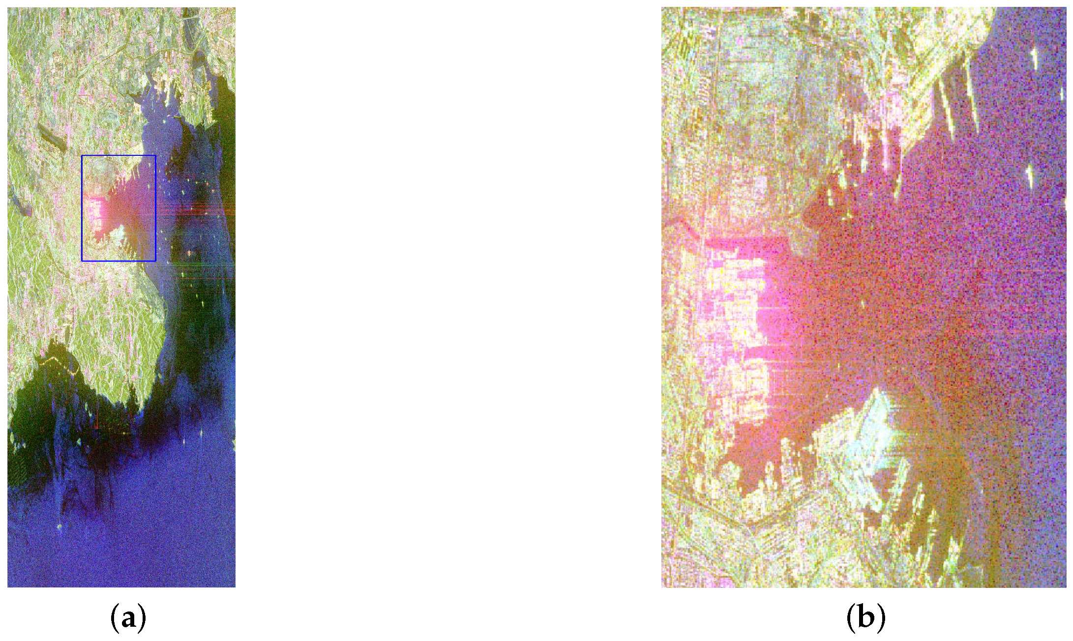
Among the three segmented regions, the water and urban areas are the regions with the minimum and maximum average scattering powers, respectively. Thus, based on the three-region MRF segmentation results, these two areas can be obtained by comparing the average total powers of the three segmented areas. However, as large harbors include large building areas with strong scattering, the echo sidelobes from the imaging process of these areas result to be superimposed on the water regions, making the scattering power of the water areas in the harbor too high and giving rise to incorrect segmentation, as shown in Figure 3, where Figure 3a shows the Pauli pseudo-color version of an image of Dalian acquired with RADARSAT-2 and Figure 3b shows the Dalian port region in the blue box in Figure 3a. The erroneous water extraction results further result in the corresponding area of the harbor not being detected correctly; therefore, the abnormal water areas need to be processed. The result of the literature [35] shows that the difference between the volume scattering power components of water areas with noise and normal ones is small, so the identification of the former can be performed by merging the results of water areas segmented according to the volume scattering power with the results of those segmented with the MRF method.

Given scattering coherency matrix T, if the surface scattering, double-bounce scattering, and volume scattering of land cover are modeled separately, with three-component decomposition, we can decompose T into the sum of the three scattering components of surface scattering, double-bounce scattering, and volume scattering [36,37,38,39].

$$T=P_s{T}_{surface}+P_d{T}_{double}+P_v{T}_{volume},$$

(5)

where $T_{surface}$, $T_{double}$, and $T_{volume}$ are the surface scattering, double-bounce scattering, and volume scattering models of the target, and $P_s$, $P_d$, and $P_v$ are the powers of the corresponding components. If Freeman three-component decomposition is used, $P_v$ equals a multiple of the cross-polarization power $\langle {\left|S_{HV}\right|}^2\rangle$, where $\langle ·\rangle$ denotes the statistical average.

To extract the abnormal water areas, we can segment the $P_v$ using the MRF method once again. However, the result segment by $P_v$ is difficult to align with the three-region MRF segmentation results. Therefore, for $P_v$, we perform the global constant false alarm rate (CFAR) threshold segmentation of the volume scattering powers of the extracted MRF-segmented water areas. Given the three-region MRF segmentation result Q, by comparing the average powers, the water area is determined as $Q_w$. By calculating the histogram of $P_v$ in region $Q_w$, under false alarm rate $Pfa$, the water and land segmentation result (B) based on $P_v$ can be obtained. On the other hand, any area that is a water area in B but not in $Q_w$ is a candidate abnormal water area, that is, abnormal water area $C=B\wedge \left(\sim Q_w\right)$, where ∧ denotes the logical AND. Further, in C, all areas D above the threshold ${Area}_{th1}$ are identified as abnormal water areas. The final result of water extraction is the concatenation of MRF-segmented water areas $Q_w$ and abnormal water areas D, that is, $E=Q_w\vee D$, where ∨ denotes the logical OR.

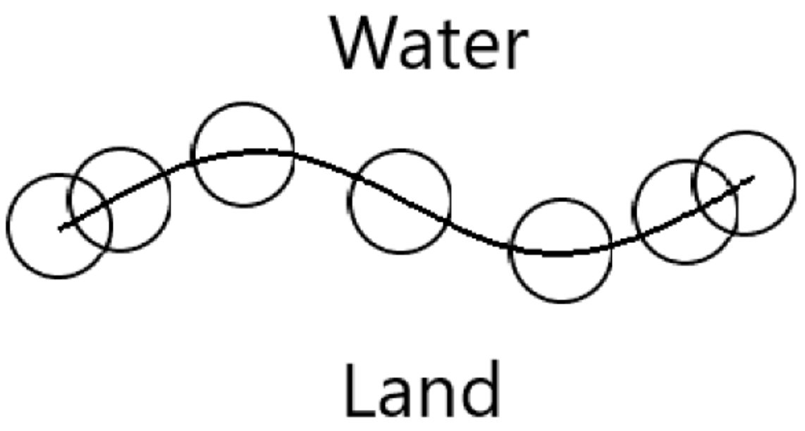
2.2. Harbor ROI Extraction

Harbors are located along the sea–land boundary, so their ROIs lie in the coastal zone region. Based on the extracted water result (E), the coastal zone region can be obtained by determining the coastline. Assuming that the maximum width of the bridge is w pixels, the sea–land segmentation result (F) can be obtained by merging the water areas in E under a distance threshold, which can be set to w. The coastline, $\left\{o_k\right\}$, can be determined from F by using the binary map boundary tracing algorithm or finding the pixel whose label is different from those of adjacent pixels. The coastal zone region is an area at a certain distance from the coastline, so with the points on $\left\{o_k\right\}$ as the centers of circles, a narrow band of the coastal zone, ${\rm Y}$, can be determined by drawing circles with distance $rad$ as the radius point by point, as shown in Figure 4.

The scattering of buildings in the harbor area is strong, so the ROIs in the harbor can be determined by extracting the strong-scattering areas with a certain area in the extracted narrow-band zone, ${\rm Y}$. Firstly, given extracted urban region $Q_u$, the strong-scattering regions in the narrow-band region (${\rm Y}$) can be obtained as $R={\rm Y}\wedge Q_u$. Then, all the connected regions in the narrow-band region, R, are identified and grouped by distance w. Finally, if the result of the grouping is $X=\left\{x_k\right\}\left(k\in \left\{1,\dots ,n_x\right\}\right)$, we can determine the minimum bounding rectangle (MBR) of $x_k$, and if the area of $x_k$ located in the MBR is larger than ${Area}_{th2}$, then it is identified as harbor ROI $y_k$. The extracted harbor ROI set is denoted by $Y=\left\{y_k\right\}\left(k\in \left\{1,\dots ,n_y\right\}\right)$.

2.3. ROI Detection Using Polarization Parameters

Because MRF segmentation is region-based and the relationship between neighboring pixels is taken into account, there can be non-artificial structures in the segmented strong-scattering urban regions. Therefore, the extracted ROIs present some false alarms, which need to be further identified by using the polarimetric scattering characteristics specific to buildings. Since buildings present reflection asymmetry compared with natural terrain, while on a horizontal–vertical orthogonal polarization basis, the co- and cross-polarization correlation coefficients (PCCs) for symmetrical target scattering are almost zero [26], that is, $〈S_{HH}{S}_{HV}^{*}〉=〈S_{HV}{S}_{VV}^{*}〉=0$, reflection symmetry can be used for final harbor detection. Correspondingly, on the circularly polarized orthogonal basis, reflection symmetry corresponds to the coefficient $〈S_{RR}{S}_{LL}^{*}〉$, where $S_{RR}\left(S_{LL}\right)$ is the right (left) hand polarization emission and right (left) hand reception scattering coefficient, and the circular polarization correlation coefficient for natural land cover is also close to 0 [28]. The horizontal–vertical polarization and circular polarization basis conversion equations are shown in (6).

$$\begin{array}{cc}\hfill S_{RR}& ={\displaystyle \frac{\left(S_{HH}-S_{VV}-j2S_{HV}\right)}{2}},\hfill \\ \hfill S_{LL}& ={\displaystyle \frac{\left(S_{VV}-S_{HH}-j2S_{HV}\right)}{2}}.\hfill \end{array}$$

(6)

For multi-look data, $〈S_{HH}{S}_{HV}^{*}〉$, $〈S_{HV}{S}_{VV}^{*}〉$, and $〈S_{RR}{S}_{LL}^{*}〉$ can be calculated based on coherency matrix T as follows:

$$\begin{array}{cc}\hfill 〈S_{HH}{S}_{HV}^{*}〉& ={\displaystyle \frac{\left(T_{13}+T_{23}\right)}{2}},\hfill \\ \hfill 〈S_{HV}{S}_{VV}^{*}〉& ={\displaystyle \frac{\left(T_{13}-T_{23}\right)}{2}},\hfill \\ \hfill 〈S_{RR}{S}_{LL}^{*}〉& ={\displaystyle \frac{\left(T_{33}-T_{22}-j\mathrm{real}\left(T_{23}\right)\right)}{2}}.\hfill \end{array}$$

(7)

where $T_{ij}$ corresponds to the i-th row and j-th column components of matrix T and $\mathrm{real}\left(·\right)$ is taken as the real part.

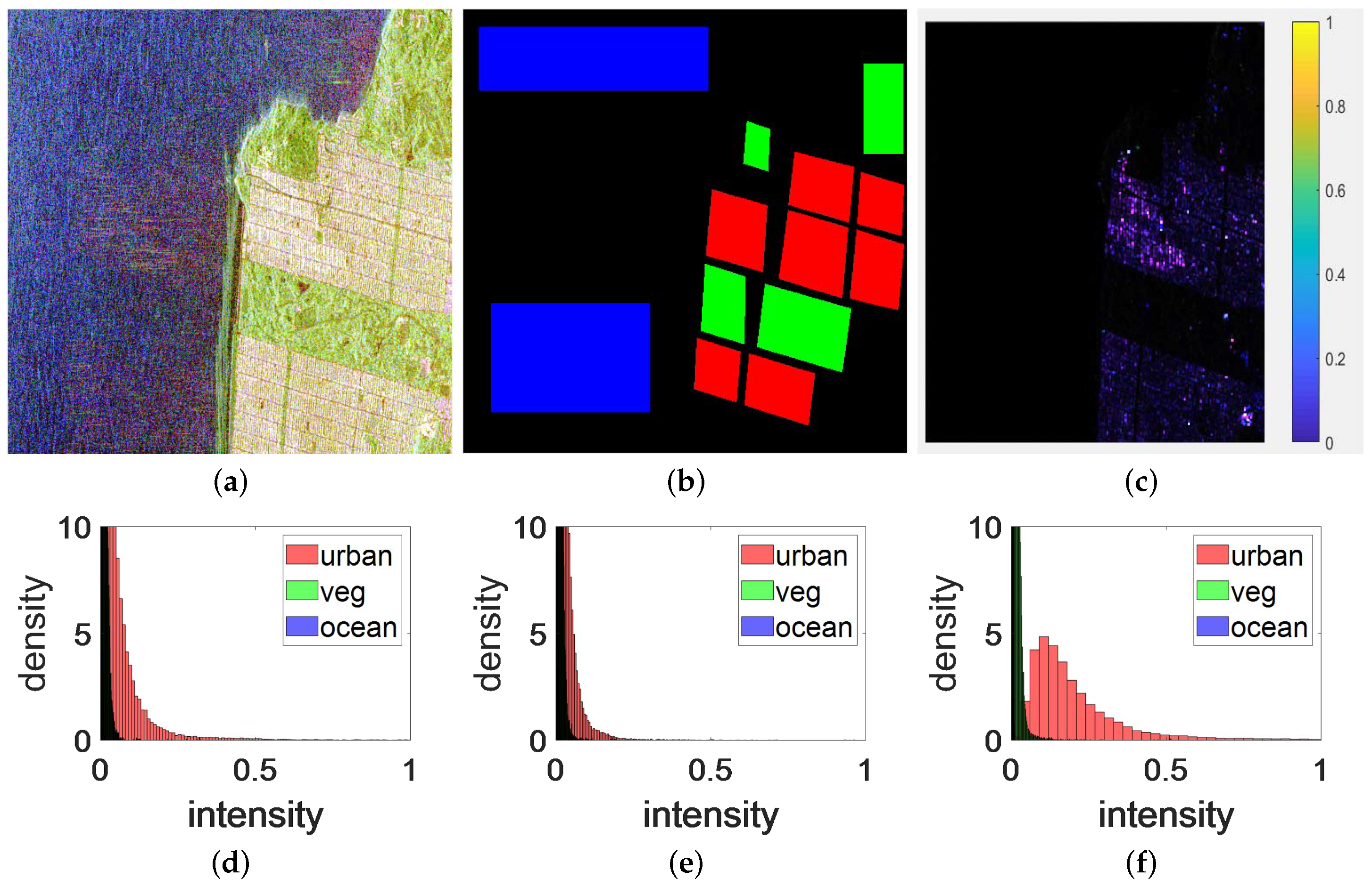
Figure 5 shows the distributions of horizontal, vertical, and circular PCCs of the polarimetric SAR image of San Francisco acquired with RADARSAT-2. Specifically, Figure 5a is the Pauli pseudo-color image; Figure 5b shows the ground truth of different regions, where the red, green, and blue regions are the masks of the urban, vegetation, and ocean categories, respectively; Figure 5c shows the pseudo-color image generated based on the three PCCs; and Figure 5d–f show the histograms of the three PCCs. We can find that the two PCCs of the natural land cover are very small but the PCCs of the urban area are greater than zero. Thus, the levels of the horizontal, vertical, and circular PCCs can discriminate between asymmetrical buildings and symmetrical land cover. However, the segmentation thresholds are also difficult to determine. Similar to the volume scattering power threshold, the thresholds of the PCCs are determined with a global CFAR method. By using vegetation region $Q_v$ in the MRF segmentation results as the background, the histogram of the PCCs in region $Q_v$ is obtained, and PCC threshold Th for asymmetric targets is determined at a set false alarm rate ($Pfa$). Image $\Omega$ is segmented by using Th as the threshold, and pixels with a PCC lower than Th are identified as asymmetric scattering regions ($\Psi$). At the same false alarm rate, global CFAR threshold segmentation is performed for the three PCCs, $〈S_{HH}{S}_{HV}^{*}〉$, $〈S_{HV}{S}_{VV}^{*}〉$, and $〈S_{RR}{S}_{LL}^{*}〉$ to determine asymmetric scattering regions ${\Psi }_1$, ${\Psi }_2$, and ${\Psi }_3$, respectively. The final asymmetric scattering region, $\Psi$, is equal to ${\Psi }_1\vee {\Psi }_2\vee {\Psi }_3$. Based on $\Psi$, the harbor ROIs can be detected. For harbor ROI $y_l$, its MBR ${Rect}_l$ is determined, and strong-scattering pixels $R_l$ of R located in ${Rect}_l$ are counted. If the percentage of pixels segmented as an asymmetric scattering region (i.e., belonging to $\Psi$) in $R_l$ is higher than $\rho$, $y_l$ is identified as a harbor.

3. Experimental Results and Analysis

The experiments were carried out on RADARSAT-2 single-look quad-polarization SAR images of Zhanjiang, Fuzhou, Lingshui, and Dalian, China; San Francisco, USA; and Singapore. The data resolution was approximately 5 m × 5 m, and the data details are shown in

Table 1. Experimental dataset details, where UTC stands for the international standard time. AOI stands for the angle of incident. $m\times m$ stands for meter times meter.

-	Scene	Size	Resolution $\left(\mathit{m}\times \mathit{m}\right)$	UTC	AOI ${(}^{\circ })$
1	Zhanjiang	$5937\times 3920$	$4.73\times 4.95$	2012-03-23 22:28:47	43.3
2	Fujian	$6140\times 3332$	$4.73\times 4.81$	2013-10-20 10:05:53	36.0
3	San Francisco	$6000\times 2800$	$4.73\times 4.82$	2008-04-09 02:01:33	28.9
4	Singapore	$6161\times 4256$	$4.73\times 4.80$	2013-01-19 11:31:08	47.4
5	Lingshui	$5421\times 3500$	$4.73\times 5.47$	2014-06-12 10:49:49	37.9
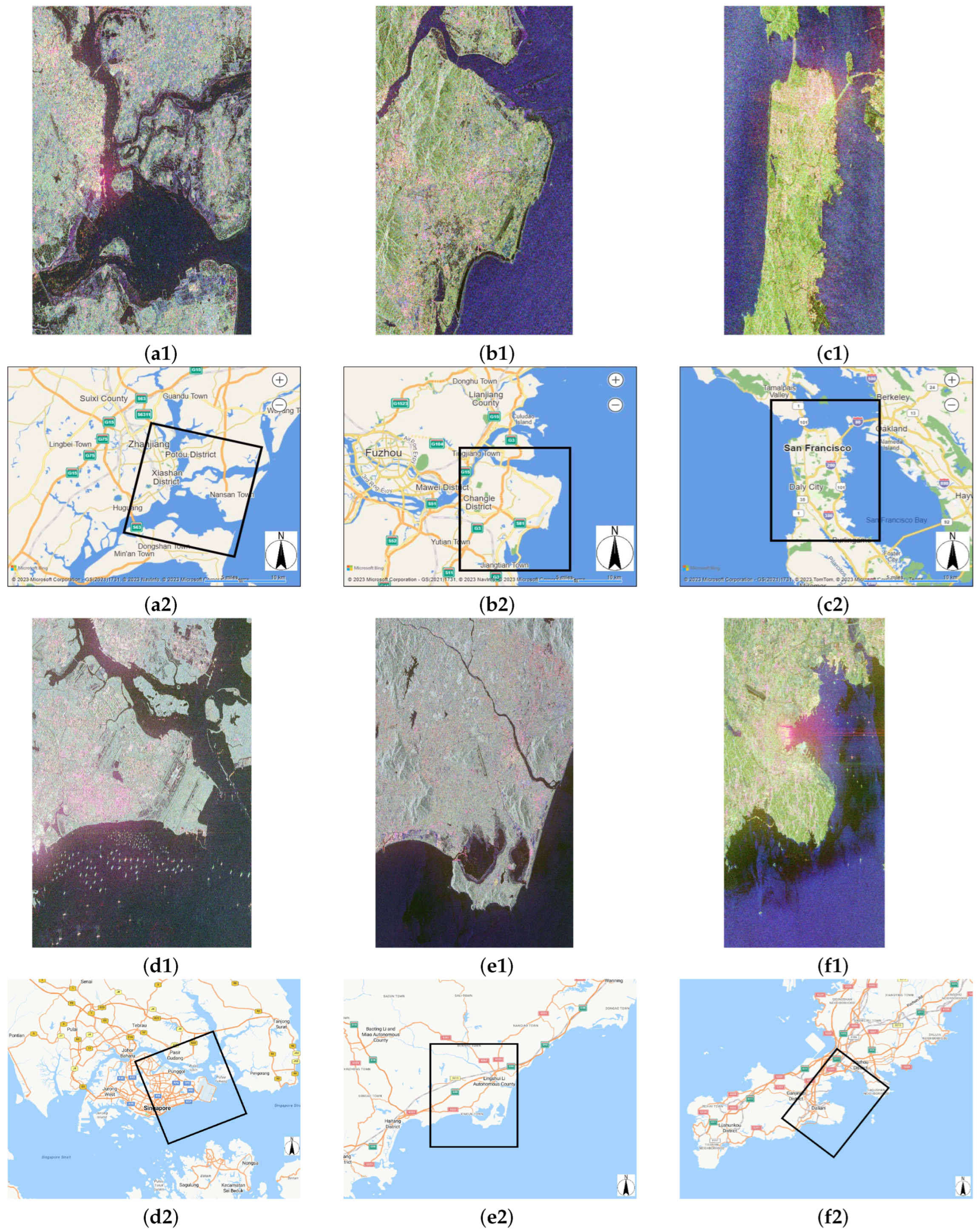
6	Dalian	$5491\times 2156$	$4.73\times 5.33$	2012-04-17 09:40:13	22.8

. Google Earth and Bing Maps were used to determine the location of the data on the map and to map the ground truth (GT) of all harbors. Figure 6 shows the Pauli pseudo-color images (Figure 6a1–f1) and the GT of the data on the map (Figure 6a2–f2).

The performance of the proposed method was evaluated with five experiments. In Experiment 1, the specific algorithm flow of the proposed method was implemented on an example image; in Experiment 2, we used images with different harbor distributions to demonstrate the robustness of the proposed method to complex scenarios; in Experiment 3, we evaluated the performance of the proposed method by using different parameter values; in Experiment 4, we performed a statistical analysis of the distribution of the co- and cross-polarization correlation coefficient powers in the harbor area; finally, in Experiment 5, we compared the performance of the proposed method with a harbor detection method based on jetty scanning. The detection rate, false detection rate, and mean intersection over union (IoU) rate were evaluated.

Given ground truth targets $\left\{G_m,m=1,\dots ,M\right\}$, where M is the number of targets, and detected targets $\left\{R_n,n=1,\dots ,N\right\}$, where N is the number of targets, the IoU between a detected target and a true target is defined as the ratio of the intersection to the union of the detected target area and the true harbor area:

$$\mathrm{IoU}={\displaystyle \frac{R_n\cap G_m}{R_n\cup G_m}},$$

(8)

where $R_n\cap G_m$ denotes the intersection of regions of $R_n$ and $G_m$ and $R_n\cup G_m$ denotes the union of the two regions.

For a true target $G_m$, if there exists a detected target $R_n$ in $\left\{R_n\right\}$ such that the IoU between $R_n$ and $G_m$ is larger than 0.5, $G_m$ is a correctly detected true target; otherwise, it is a missed target. For a detected target $R_n$, if there exists a true target $G_m$ in $\left\{G_m\right\}$ such that the IoU between $R_n$ and $G_m$ is greater than 0.5, $R_n$ is a correctly detected target; otherwise, it is a false alarm. The detection rate is defined as the ratio of the number of correctly detected true targets, $M_t$, to the number of true targets, M, and the false rate is defined as the ratio of the number of false alarm detected targets, $N_f$, to the number of detected targets, N [40], i.e.,

$$\begin{array}{cc}\hfill \mathrm{Pd}& ={\displaystyle \frac{M_t}{M}},\hfill \\ \hfill \mathrm{Pf}& ={\displaystyle \frac{N_f}{N}}.\hfill \end{array}$$

(9)

Because the proposed method allows for the detection of harbors along the coastline one by one, the number of correctly detected targets, $N_t$, is equal to the number of correctly detected true targets, $M_t$. The mean IoU (mIoU) between the detected targets and the true targets is defined as the ratio of the area intersection to the union of the correctly detected targets and the true targets [41], i.e.,

$$\mathrm{mIoU}={\displaystyle \frac{{\sum }_{k=1}^{N_t}D{R}_k\cap D{G}_k}{{\sum }_{k=1}^{N_t}D{R}_k\cup D{G}_k}},$$

(10)

where $D{R}_k$ denotes the kth correctly detected target and $D{G}_k$ denotes the corresponding kth ground truth target.

According to the description of the method in Section 2, the parameters of the proposed method were determined and are summarized in

Table 2. Parameter list of proposed method.

Module	Function	Parameter	Value
Prior constant	Image resolution	$R_x\times R_y$	Read from data header file
	Maximum jetty width	W	100 m
	Jetty width pixels	$\omega$	$W/\sqrt{\left(R_x^2+R_y^2\right)/2}$
	Multi-look process	$\mathcal{L}$	5
	Jetty width pixels in multi-look image	w	$\omega /\mathcal{L}$
Water and urban region extraction	Gibbs distribution parameter	$\beta$	0.5
	Area threshold for abnormal water area detection	${Area}_{th1}$	${\mathcal{L}}^2{w}^2$
ROI extraction	Narrow-band radius	$rad$	$\left(w+\mathcal{L}-1\right)/2$
	Area threshold for strong-scattering extraction	${Area}_{th2}$	$w^2$
ROI detection	Constant false alarm rate	$Pfa$	0.01
	PCC area ratio threshold	$\rho$	0.4

. In the water and urban region extraction step, two parameters are used: the Gibbs distribution parameter ($\beta$) for three-region MRF segmentation and the area threshold (${Area}_{th1}$) for abnormal water area determination. Similarly, in the ROI extraction step, two parameters are employed: the radius ($rad$) for the extraction of the coastal narrow-band zone and the area threshold (${Area}_{th2}$) for the strong-scattering extraction of the narrow-band zone. Finally, in the ROI detection step, two parameters are used: the false alarm rate ($Pfa$) and the PCC area ratio threshold ($\rho$). To adapt the parameters to data acquired with different sensors, we set the constant parameter of jetty width, W, based on prior knowledge. Assuming that the image resolution is $R_x\times R_y$ and the maximum width of jetty W is 100 m, then the number of pixels of the jetty width, $\omega$, is obtained as $W/\sqrt{\left(R_x^2+R_y^2\right)/2}$. Considering that harbors are usually large in size, the input data were $\mathcal{L}\times \mathcal{L}$ multi-look processed (the value taken in our experiment was 5); under these conditions, the maximum number of pixels of the jetty width is $w=\omega /\mathcal{L}$. If the detected MBR of the harbor under multi-look data conditions is ${Rect}_l$, its corresponding position in the original image can be simply determined by expanding ${Rect}_l$$\mathcal{L}$ times. For MRF segmentation, the Gibbs distribution parameter, $\beta$, was set to 0.5. For extracting the water areas, the area threshold for determining abnormal water areas, ${Area}_{th1}$, was set to ${\mathcal{L}}^2{w}^2$. For extracting the harbor ROIs, the radius for the extraction of the narrow-band zone, $rad$, was set to $\left(w+\mathcal{L}-1\right)/2$. Assuming that the length and width ranges of the MBR in the narrow-band zone are at least w in size for strong scattering, the area threshold for strong-scattering extraction in the narrow-band zone, ${Area}_{th2}$, was taken as $w^2$. For harbor detection, the false alarm rate, $Pfa$, was set to 0.01 and the PCC area ratio threshold, $\rho$, to 0.4. The values of w, $Pfa$, and $\rho$ were determined according to the performance of the proposed method with the parameters in Experiment 3.

3.1. Illustration of Algorithm Flow

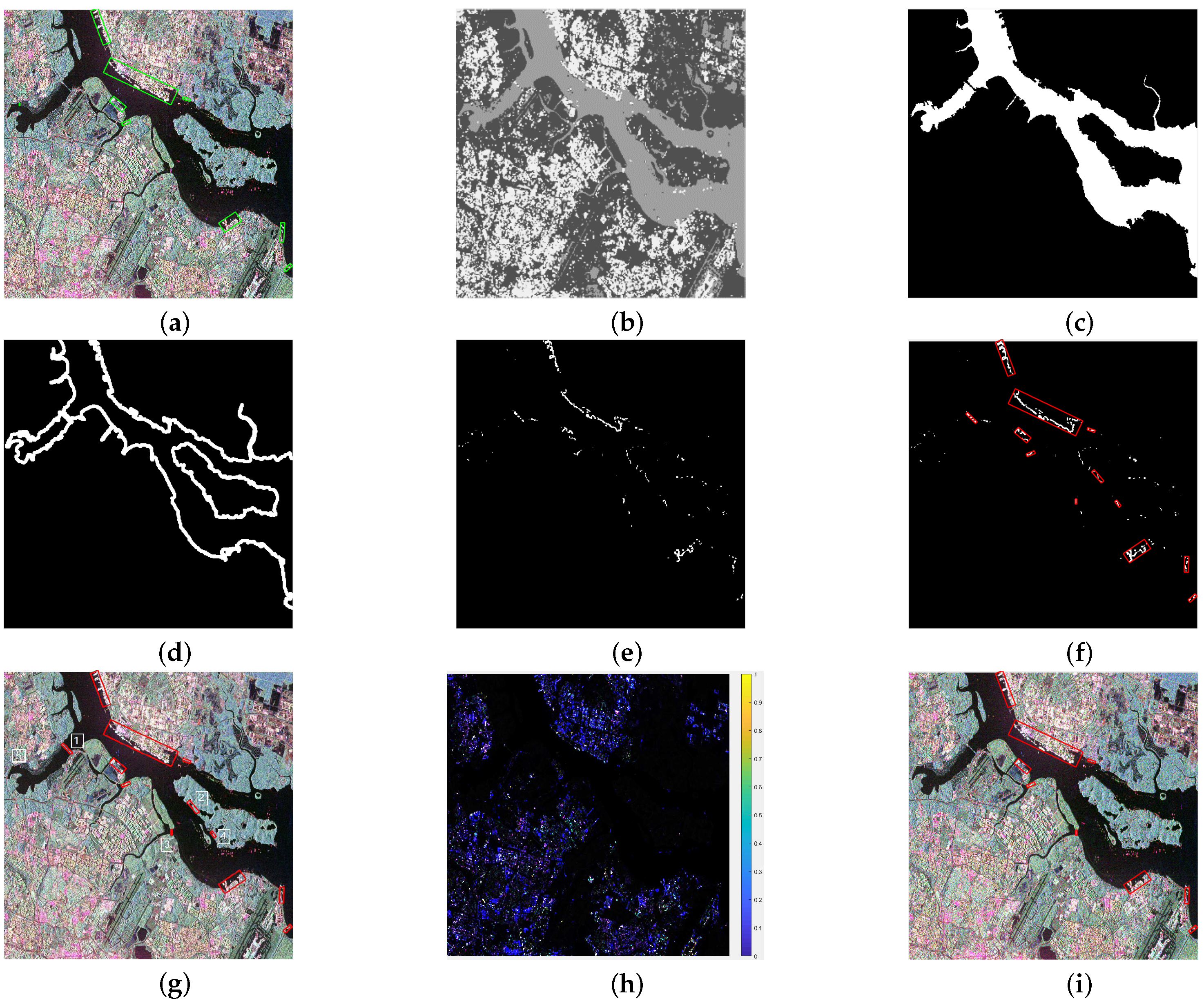
The process results of the proposed method are illustrated here by using part of image 4 in Table 1. Figure 7a shows the Pauli pseudo-color image and the GT of the harbors, where the harbors are marked with green boxes. We can observe that there are several harbors of different shapes along the coast and that the harbor jetties are relatively small and their geometric features very vague; some of the large harbor jetties are mixed with buildings along the coast, while some of the small harbor jetties are irregular in shape, so using a harbor detection method based on geometric features would result in several missed targets. The common features of these geometrically diverse harbors are their being surrounded by water and their presenting several strong-scattering artificial structures on land. Figure 7b–i show the detection results obtained with the proposed method. Among them, Figure 7b shows the three-region segmentation results after the processing of abnormal water areas. By comparing Figure 7a,b, we can find that both water areas and strong-scattering buildings were well-segmented, and following the extraction of the volume scattering powers for segmentation, the water and strong-scattering building areas presenting interference were correctly segmented. Figure 7c shows the water area results extracted from the three-region segmentation results, which indicate that the water areas associated with the harbors were correctly extracted. Figure 7d shows the narrow-band area of the coastal zone determined according to the water–land boundary line. Figure 7e shows the distribution of strong scattering in the coastal narrow-band area. By comparing Figure 7a and Figure 7e, we can find that the strong-scattering artificial structures along the shoreline of each harbor, including jetties, docked ships, and bridges, were included in the extracted coastal narrow-band area. Figure 7f shows the detected harbor ROIs, and Figure 7g shows their location in the Pauli pseudo-color image, where the harbor ROIs are marked with red boxes and the detected false targets with white numbered rectangular boxes. By comparing Figure 7a and Figure 7g, we can see that eight harbors of varying morphology were correctly detected as harbor ROIs, except the small harbor in region 5; however, as large sea-crossing bridges are also areas with strong scattering, the detected ROIs contain some false alarms, such as regions 1–4 (Figure 7g). Figure 7h shows the pseudo-color image generated based on the horizontal, vertical, and circular co-polarization PCC powers. We can find that the correlation powers of asymmetric targets such as the buildings in the harbor area are significantly higher than those of asymmetric areas such as vegetation and soil regions. Figure 7i shows the final harbor detection results. By comparing Figure 7g and Figure 7i, we can find that false alarms 1, 2, and 4 in Figure 7g were effectively eliminated, indicating that the proposed method allowed for the correct detection of eight harbors with only one missed target and one false alarm.

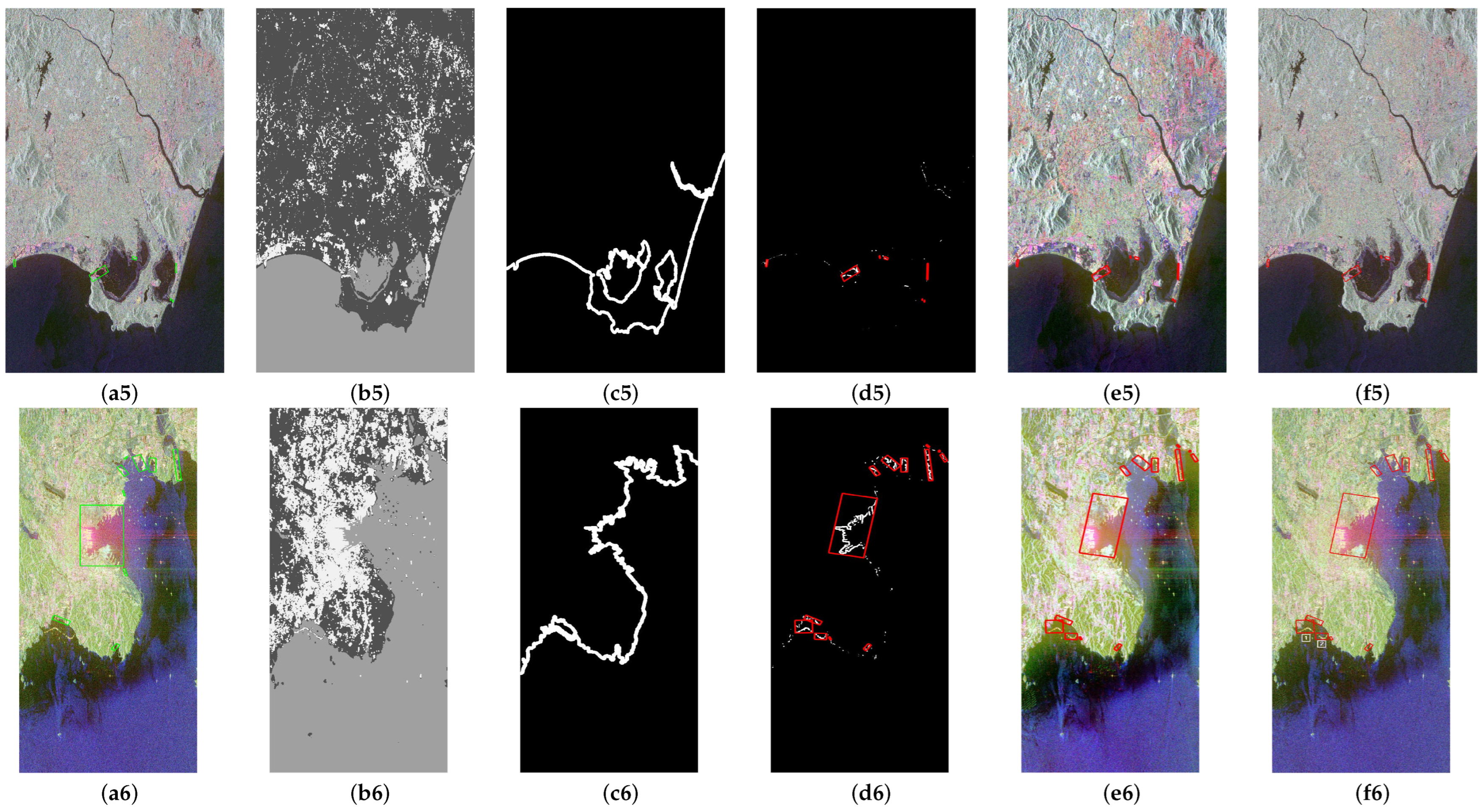
3.2. Performance in Different Harbor Scenarios

The performance of the proposed method was evaluated in different harbor distribution scenarios by using images 1–6 in Table 1. The test results are shown in Figure 8, where Figure 8(ai–fi) correspond to the results for image i. Figure 8(a1–a6) show the Pauli pseudo-color images and the GT of the harbors. Analyzing the regional distribution of the harbors reveals significant differences in their distributions and backgrounds in the three datasets. In the Zhanjiang region, there are several T-shaped and $\pi$-shaped harbors with regular geometrical structures, and there are also several harbors without jetties. In the Fuzhou area, the harbor jetties are relatively small and mixed with artificial structures along the coast, with very vague geometric features. In the San Francisco area, there are a large number of harbors and jetties along the coast, some of which span a large area and are close to each other, with varying structures and irregular geometric profiles. In the Singapore region, there are many harbors of different shapes, some of which are small and irregular in shape and some of which are large and mixed with buildings along the coast. In the Lingshui region, most harbors are located around the inland waters, without any jetties or breakwaters. In the Dalian region, there is a large port located in the center of the image, where the surrounding water presents noise derived from strong echo sidelobes. Based on the background sea and land areas, the sea is relatively rough in Fuzhou, San Francisco, Singapore, and Dalian; while this is less true for Zhanjiang and Lingshui, there are a large number of aquaculture ponds along the coast and aquaculture installations at sea. It is very difficult to detect harbors in these types of areas, as they present irregular harbor distributions and complex backgrounds. Figure 8(b1–b6) show the water and urban region extraction results. We can observe that the water, vegetation, and strong-scattering artificial structure areas were well-segmented and that the coastal harbor water areas presenting strong-scattering interference were also correctly processed. Figure 8(c1–c6) show the coastal narrow-band zone determined according to the coastline. Figure 8(d1–d6) show the harbor ROIs determined from the regions of strong scattering in the narrow-band zone. By comparing these results with the GT of the harbors, we can find that the building areas of interest near the coastal harbors were correctly extracted. Figure 8(e1–e6) show the detected harbor ROIs in the Pauli pseudo-color image. Figure 8(f1–f6) show the harbor regions identified according to the co- and cross-polarization correlation powers. By comparing these results with Figure 8(a1–a6), we can find that the harbor regions of varying morphology and size were all effectively detected. Due to the distribution of several other strong-scattering structures along the coast, which also have high PCC powers, some false alarms can be found in all three datasets. Because bridge areas comprise the coast as well as the sea and present a large number of strong-scattering artificial structures, there were false alarms along the sea-crossing bridges in Zhanjiang, San Francisco, and Dalian, as shown in Figure 8(f1), area 1; Figure 8(f3), area 1; and Figure 8(f6), areas 1 and 2. Due to the integration of the sea-crossing bridges into the large harbors on both sides, there were also missed targets for the large harbors on both sides of the sea-crossing bridge in the San Francisco area, as shown in Figure 8(f3), areas 2 and 3.

Table 3. Performance evaluation in different scenarios, where Num indicates the number of actual harbors, Correct is the number of correctly detected harbors, False indicates the number of false alarm harbors, Pd is the detection rate, Pf is the false detection rate, and mIoU is the mean intersection over union rate.

Image	Num	Correct	False	Pd (%)	Pf (%)	mIoU
1	26	23	6	88.5	20.7	0.767
2	13	12	6	92.3	33.3	0.762
3	12	7	7	58.3	50.0	0.467
4	26	23	14	88.5	37.8	0.631
5	6	6	1	100	14.3	0.892
6	10	7	6	70.0	46.1	0.600

lists the detection performance of the three datasets. Out of the 26 harbors distributed in the Zhanjiang region, with the proposed method, 23 harbors were correctly detected, with a detection rate of 88.5% and a false detection rate of only 20.7%. Out of the 13 harbors in the Fuzhou region, 12 harbors were correctly detected, with a detection rate of 92.3% but a false detection rate of 33.3%. All six harbors in the Lingshui region were correctly detected, with only one false alarm. Out of the 26 harbors in the Singapore region, 23 harbors were correctly detected, but there were 14 false alarms due to the coastal bridges and buildings. The tested mIoU indexes of the Zhanjiang, Fuzhou, and Lingshui results were above 0.76. The detection rates, false detection rates, and mIoU indexes for the San Francisco and Dalian areas were all poor, mainly because of the sea-crossing bridges.

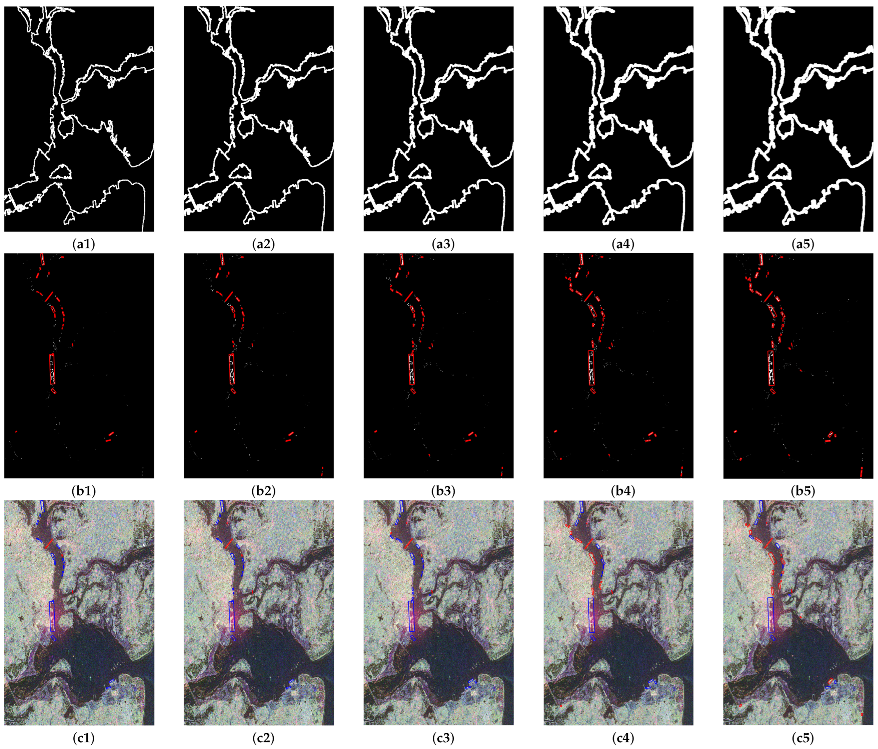
3.3. Results for Different Parameter Values

The performance of the proposed method was compared by using different parameter values. Firstly, we changed the narrow-band radius. If we assume that the width of a jetty (W) is 100 m, the narrow-band radius ($rad$) can be calculated to be 4 pixels, so in the experiments, $rad$ was set to 2, 3, 4, 5, and 6 pixels. The experimental results for the Zhanjiang area for different $rad$ values are shown in Figure 9, where Figure 9(ai–ci) correspond to the experimental results for radius i + 1. For different radii, Figure 9(a1–a5) show the coastal narrow-band area, Figure 9(b1–b5) the extracted harbor ROIs, and Figure 9(c1–c5) the detected harbor areas, where the correctly detected targets are marked in blue and the false alarms in red. We can observe that as the radius increased, the narrow-band area gradually became wider, the building area in the extracted harbor ROIs gradually increased, and the number of small harbors detected increased.

Table 4. Performance comparison with different narrow-band radii for image of Zhanjiang. $rad$ denotes the narrow-band radius.

rad	Num	Correct	False	Pd (%)	Pf (%)	mIoU
2	26	17	3	65.4	15.0	0.643
3	26	19	4	73.1	17.4	0.675
4	26	23	6	88.5	20.7	0.767
5	26	14	15	53.8	51.7	0.602
6	26	12	19	46.2	61.3	0.552

shows the variation in performance with different radii. The results show that as the radius increased, the number of correctly detected targets increased from 17 at a radius of 2 to 23 at a radius of 4, and the number of false alarm targets increased from 3 at a radius of 2 to 6 at a radius of 4, while the mIoU indexes of the detected targets increased from 0.643 to 0.767. As the radius increased, the number of targets detected increased from 29 at a radius of 4 to 31 at a radius of 6, but the number of correctly detected targets decreased significantly; further, the number of false alarms increased significantly from 6 at a radius of 4 to 19 at a radius of 6, while the mIoU rate decreased. The reason for this is that, as the radius increases, the percentage of total pixels of strong-scattering artificial structures in the narrow-band area of small harbors decreases, leading to missed targets, while the percentage of total pixels of strong-scattering artificial structures along the coast increases, leading to false alarms.

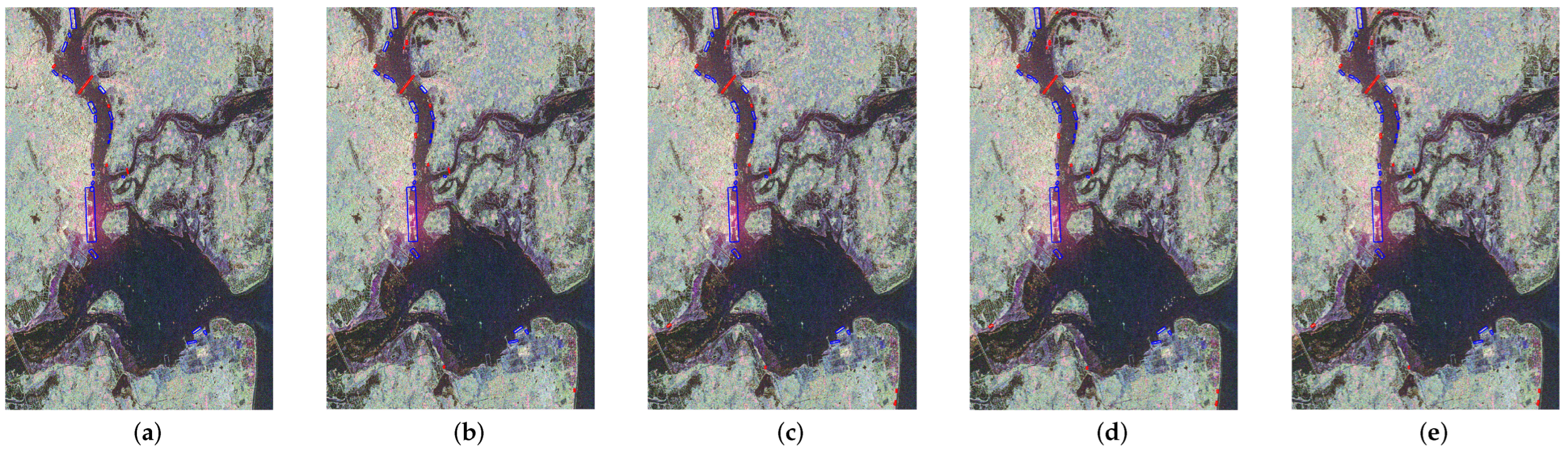
The performance of the proposed method was then evaluated by using different false alarm rates ($Pfa$), and the experimental results for the Zhanjiang region are shown in Figure 10. Figure 10a–e correspond to the results with $Pfa$ of 0.01, 0.02, 0.05, 0.08, and 0.1, respectively, where the correctly detected targets are marked in blue and the false alarms in red. The results show that the false alarms increased as $Pfa$ increased.

Table 5. Performance comparison with different false alarm rates for image of Zhanjiang, where $Pfa$ denotes the false alarm rate.

Pfa	Num	Correct	False	Pd (%)	Pf (%)	mIoU
0.01	26	23	6	88.5	20.7	0.767
0.02	26	23	12	88.5	34.3	0.757
0.05	26	23	14	88.5	37.8	0.748
0.08	26	23	14	88.5	37.8	0.748
0.10	26	23	14	88.5	37.8	0.748

shows the variation in performance for different $Pfa$. The results show that as $Pfa$ increased, the number of false alarms increased from 6 at a $Pfa$ of 0.01 to 14 at a $Pfa$ of 0.05, while for higher $Pfa$, the number of false alarm targets remained the same; as $Pfa$ changed, the mIoU indexes remained almost unchanged, close to 0.75 in all cases. These results are mainly due to the fact that, as $Pfa$ increases, more pixels in the harbor ROIs are classified as target pixels, thus making some of the non-harbor buildings being incorrectly classified as harbor targets.

Finally, the performance of the proposed method was evaluated by using different area ratio thresholds ($\rho$). The results for the image of Zhanjiang with different thresholds are shown in Figure 11. Figure 11a–e correspond to the results for $\rho$ of 0.3, 0.4, 0.5, 0.6, and 0.7, respectively; in the figure, the correctly detected targets are marked in blue, and the false alarms in red.

Table 6. Performance comparison with different area ratio thresholds for image of Zhanjiang, where $\rho$ indicates the area ratio thresholds.

$\mathsf{\rho }$	Num	Correct	False	Pd (%)	Pf (%)	mIoU
0.3	26	23	11	88.5	32.4	0.751
0.4	26	23	6	88.5	20.7	0.767
0.5	26	21	6	80.8	22.2	0.743
0.6	26	20	4	76.9	16.7	0.743
0.7	26	16	2	61.5	11.1	0.680

shows the variation in performance with different $\rho$ values. We can observe that as the threshold value increased, the number of detected targets, both correct targets and false alarms, gradually decreased. The detection rate decreased from 88.5% at a $\rho$ of 0.3 to 61.5% at a $\rho$ of 0.7, while the false alarm rate decreased from 32.4% at a $\rho$ of 0.3 to 11.1% at a $\rho$ of 0.7. The reason for this is that as the threshold increases, the pixel proportion of high PCC powers in the harbor ROIs gradually decreases, resulting in a reduction in both the number of detected targets and false alarms.

3.4. Statistics of Different PCC Powers

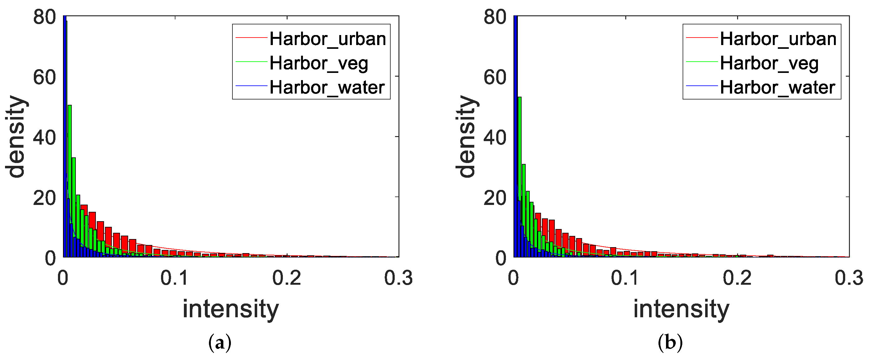
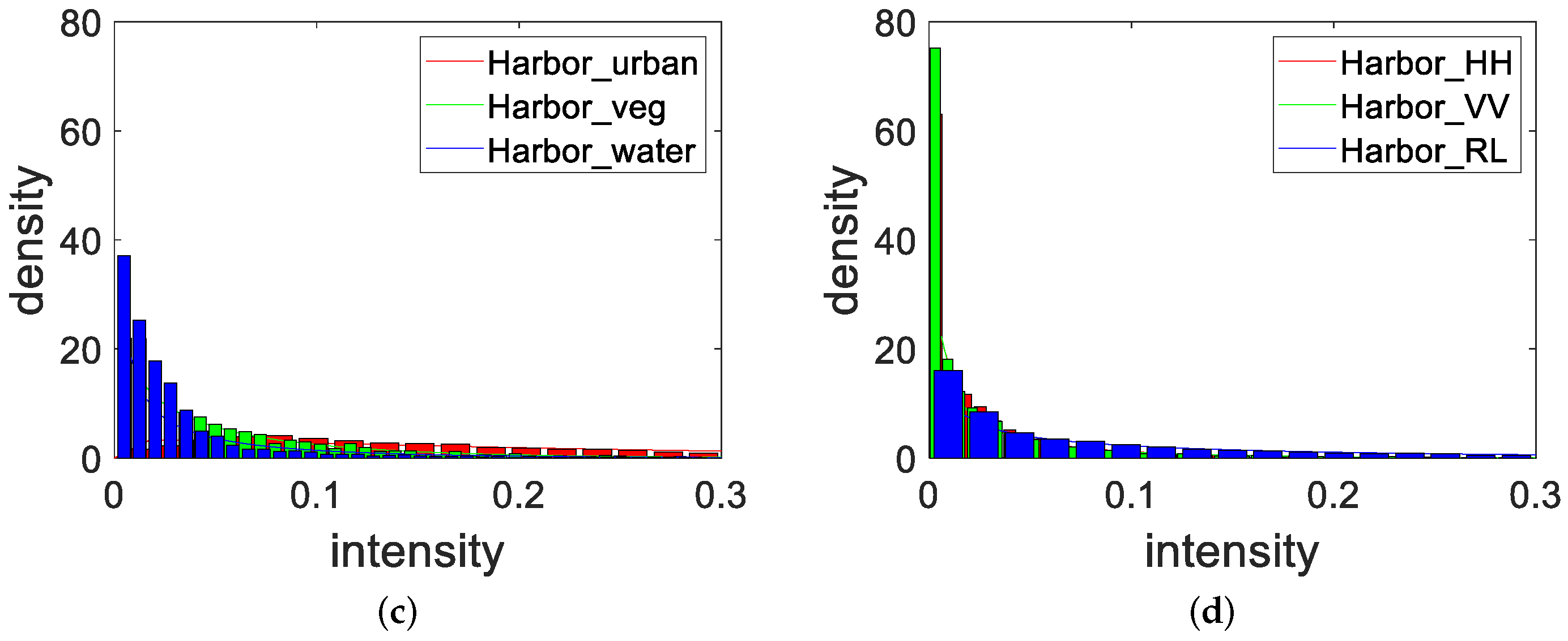
To assess the validity of the polarization parameters in the proposed method, a statistical analysis of the different polarization parameters in the harbor area was carried out. Firstly, the histograms of horizontal, vertical, and circular co- and cross-polarization correlation powers for the harbor water, vegetation, and building areas were obtained, as shown in Figure 12, where for the three regions (Harbor_urban for buildings, Harbor_veg for vegetation, and Harbor_water for water), Figure 12a–c show the histograms of the horizontal, vertical, and circular PCC powers, respectively. From Figure 12a,b, we can see that the horizontal and vertical PCC powers of the three regions were significantly different. From Figure 12c, we can see that the difference in the circular PCC powers of water and vegetation was small, but there was a difference in circular PCC power between these two features and the harbor building area. Therefore, with vegetation as a background, global CFAR detection can be performed, and based on the determination of thresholds, building areas can be successfully separated from other areas. Figure 12d shows the histogram of the three different PCC powers in the harbor area, where Harbor_HH, Harbor_VV, and Harbor_RL indicate horizontal, vertical, and circular polarization, respectively. We can observe that the histograms of the three different PCC powers almost overlap.

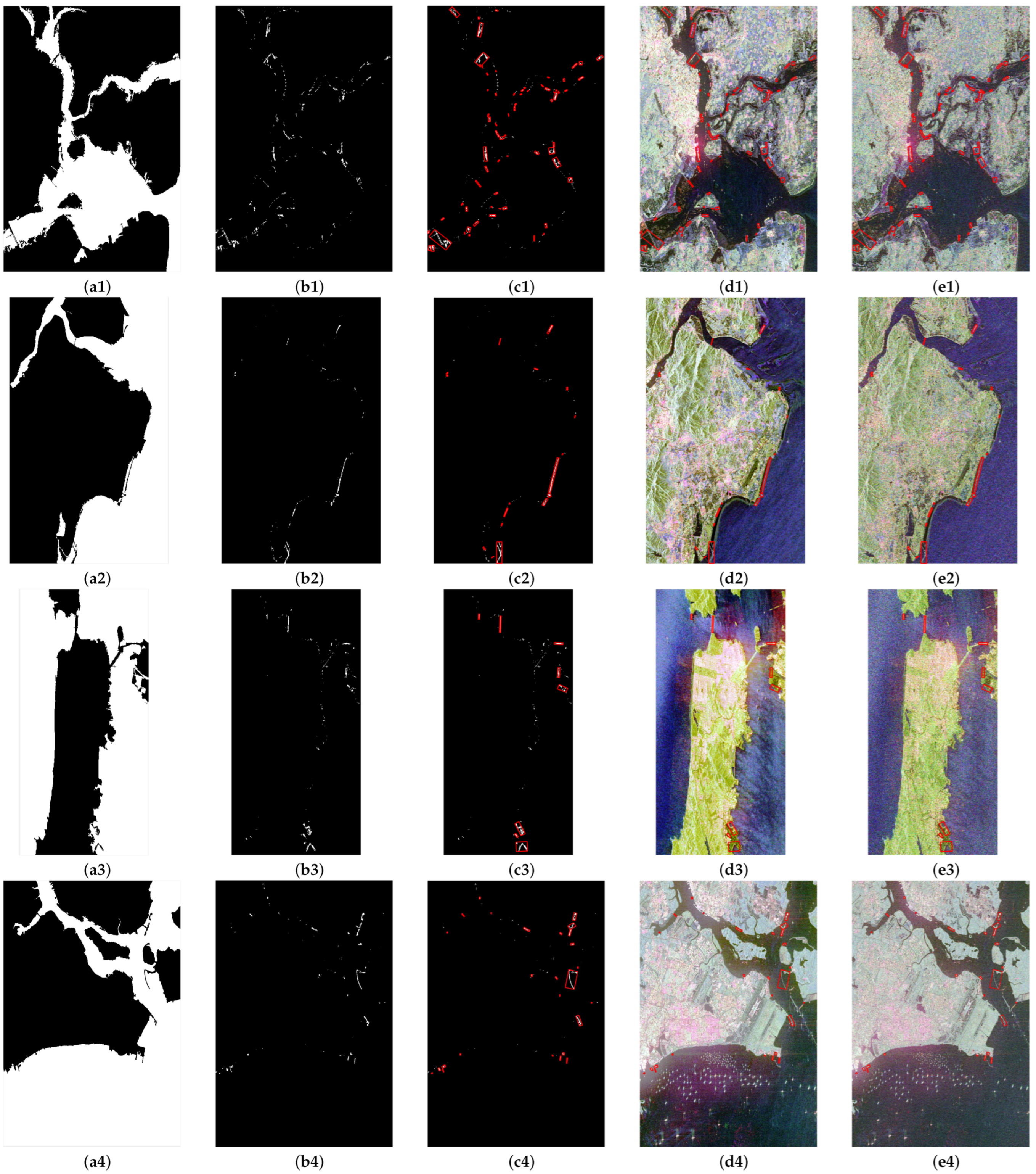
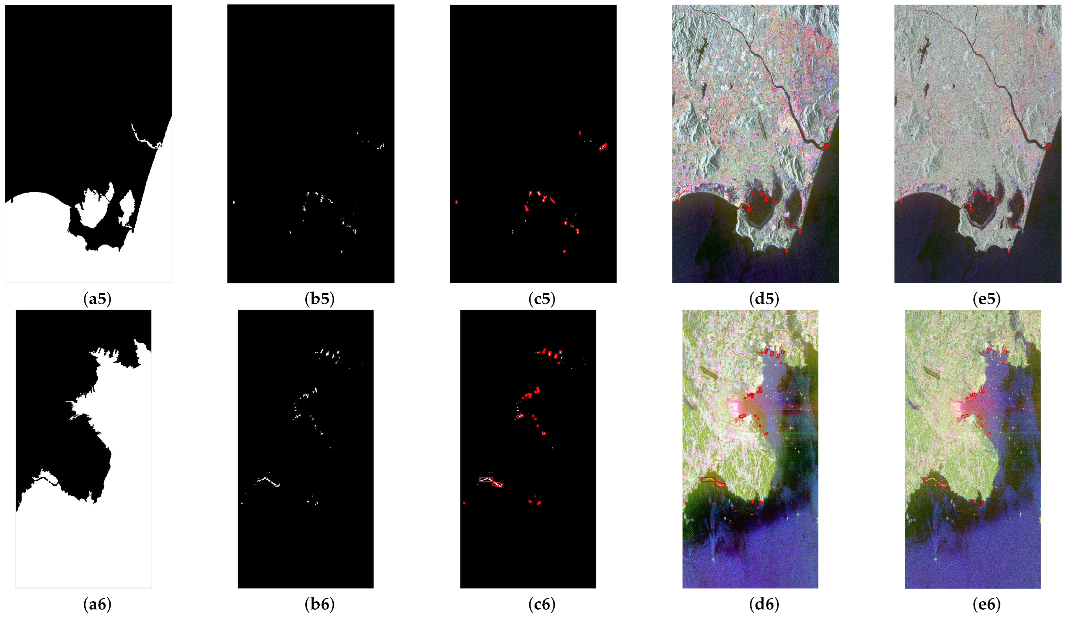
3.5. Performance Comparison with a Spatial Method

The proposed method was compared with a harbor detection method based on jetty scanning [15,33]. Figure 13 shows the results for images 1–6 in Table 1 obtained by using the comparison method, where Figure 13ai–ei correspond to the results of image i. Figure 13(a1–a6) show the water extraction results of the proposed method obtained by using multi-look data. Figure 13(b1–b6) show the scanning results based on two pairs of orthogonal directional jetties, where we can observe that all the raised areas along the coast were scanned out. Figure 13(c1–c6) show the harbor areas detected based on the merging of the scanned jetties within distance w. Figure 13(d1–d6) show the results of the corresponding areas in the Pauli pseudo-color versions of the multi-look images. Figure 13(e1–e6) show the corresponding detection results in the Pauli pseudo-color images. The results show that there were a large number of false alarms for the images of Zhanjiang, Singapore, and Dalian because of the numerous raised areas along the coast, and multiple jetties in large ports were detected as single harbors; on the other hand, only a small number of harbors were detected in the images of Fuzhou, San Francisco, and Lingshui due to the raised jetties not being sharp enough and being mixed with artificial structures along the coast.

Table 7. Performance of jetty scanning method on images 1–6.

Image	Num	Correct	False	Pd (%)	Pf (%)	mIoU
1	26	2	66	7.7	97.0	0.047
2	13	0	17	0	100	0.005
3	12	1	7	8.3	87.5	0.027
4	26	5	21	19.2	80.7	0.092
5	6	1	14	16.7	93.3	0.019
6	10	0	23	0	100	0.037

lists the detection performance on the six images, showing that the detection rates were less than 20%, the false detection rates were greater than 80%, and the mIoU metrics were all less than 0.1 in all cases. By comparing the results in Table 2, we can find that the performance of the proposed method was much better than that of the comparison method.

4. Discussion

In this study, we established a novel method for polarimetric SAR image harbor detection based on context features and reflection symmetry. By extracting the statistical and polarimetric scattering features of the waters and buildings of harbors, harbor detection is achieved by extracting the water areas of interest, the coastal narrow-band zone area, the strong-scattering building areas, and the non-reflection symmetric strong-scattering areas step-by-step. As it does not rely on the extraction of harbor geometric features, this method prevents the problem encountered in traditional spatial methods, with which geometric features are difficult to detect due to the variety of harbor morphology.

One of the common features of harbors with different morphology is that they are all located at the land–water boundary. Based on the difference in the scattering coherency matrices of water areas, strong-scattering built-up areas, and vegetation areas, an MRF segmentation method based on the statistical properties of the area is used to segment the analyzed features and classify them as low-scattering areas, strong-scattering areas, or other areas. Water areas are initially extracted based on the results of low-scattering area segmentation. However, considering the results of the six images in the experiment, for scenes with complex harbor distributions, the coastal water areas present noise derived from the secondary echoes formed by strong scattering from buildings along the coast. Since the noise of the volume scattering power of these water areas is trivial, the latter areas can be processed by segmenting the volume scattering power obtained with three-component decomposition. The experimental results show the accuracy of water area extraction post-processing.

Another common feature of different harbors is that there exist a large number of buildings on land, giving rise to large areas with strong scattering and complex scattering components. By extracting the large strong-scattering areas in the coastal narrow-band zone, the harbor ROIs can be extracted effectively, regardless of the different harbor sizes, contour shapes, and building distributions. The results of the different harbor distribution scenarios in Experiment 2 show that the harbor ROIs can be extracted effectively with our method. Since the horizontal, vertical, and circular co- and cross-polarization correlation power parameters can effectively discriminate between asymmetric and symmetric scattering regions, the false alarms in the detected harbor ROIs can be effectively screened out.

The proposed method can be applied for the detection of harbors of different sizes and types because it is not based on extracting the geometrical features of the harbor contours. By comparing the proposed method with the spatial jetty scanning harbor detection method, we found that the former has much better detection rates, false detection rates, and mIoU rates. However, the experimental results also show that with the proposed method, some false alarms were obtained due to the presence of non-harbor artificial structures and sea-crossing bridges. Further, the experimental results for the images of San Francisco and Dalian show that using the proposed method may not allow for the detection of large harbors due to the presence of large sea-crossing bridges and may result in the mixing of several harbor areas into one.

5. Conclusions

In this study, we developed a method for harbor detection in polarimetric SAR images based on context feature detection and co- and cross-polarization correlation power discrimination. By leveraging the contextual features that harbor areas are surrounded by water and that nearby buildings form a large area with strong scattering, the image is segmented into low-scattering water areas, strong-scattering urban areas, and other areas with three-region MRF segmentation. Based on the segmentation results of the low-scattering regions, the water areas affected by noise deriving from the coastal strong-scattering building areas are determined by segmenting the volume scattering powers, preventing the incorrect segmentation of these areas. Based on the water boundary line, the narrow-band region of interest of the harbor is extracted, and the harbor ROIs are extracted by determining the strong-scattering urban area in the large area of the narrow-band region, which effectively prevents the problem of difficult feature extraction caused by different harbor morphology and the lack of common features. Finally, harbors are effectively identified by leveraging the asymmetric scattering characteristics of the harbor building areas while combining the horizontal, vertical, and circular co- and cross-polarization correlation powers. The experimental results for multiple RADARSAT-2 polarimetric SAR images demonstrate the effectiveness of the proposed method. For scenes with complex harbor morphology and background distribution, the proposed method allowed for accurate detection, and its performance was found to be far better than that of a traditional spatial harbor detection method.