A Deep-Learning Based GNSS Scene Recognition Method for Detailed Urban Static Positioning Task via Low-Cost Receivers

Abstract

Global Navigation Satellite Systems (GNSS)-based position service is widely applied in cities, but the precision varies significantly in different obstruction scenes. Scene recognition is critical for developing scene-adaptive GNSS algorithms. However, the complexity of urban environments and the unevenness of received signal especially in low-cost receivers limit the performance of GNSS-based scene recognition models. Therefore, our study aims to construct a scene recognition model suitable for urban static positioning and low-cost GNSS receivers. Firstly, we divide the scenes into five categories according to application requirements, including open area, high urban canyon, unilateral urban canyon, shade of tree and low urban canyon. We then construct feature vectors from original observation data and consider the geometric relationships between satellites and receivers. The different sensitivity to different scenes is discovered through an analysis of the performance of each feature vector in recognition. Therefore, a GNSS positioning scene recognition model based on multi-channel LSTM (MC-LSTM) is proposed. The results of experiments show that an accuracy of 99.14% can be achieved by our model. Meanwhile, only 0.75 s and 1.95 ms are required in model training per epoch and model prediction per data on a CPU, which presents a significant improvement of over 90% compared with existing works. Furthermore, our model can be transferred into different time periods quickly and can maintain robustness in situations where one or two types of observation data are missed. A maximum accuracy of 81.13% can be achieved when two channels are missed, while 96.06% is attainable when one channel is missed. Therefore, our model has the potential for real applications in complex urban environments.

1. Introduction

Global Navigation Satellite Systems (GNSS) have undergone rapid development and progress in past decades. With the successive establishment of global services such as GPS, BDS, GLONASS, Galileo and regional services such as QZSS, IRNSS, GNSS-based applications have also widely been implemented. Bike-sharing is a typical example among them. Due to its convenience for short-length travel and last-mile connectivity of public transportation, bike-sharing services have expanded to over 300 cities in mainland China and gained widespread popularity especially in super cities [1]. However, the prosperous growth of bike-sharing has brought a series of problems. Over-deployment by operators, false-parking by users and poor scheduling by public management have caused mass disarray of public sharing-bikes, which has become a hot and troubling issue among citizens [2].

A practical solution to this problem is to use electronic fence technology to regulate users’ parking behaviors, which means the bike-sharing service is made unable to deactivate unless they are parked in the range of virtual “parking zones”. Unfortunately, shared bikes often need to be parked in complex environments, which means GNSS signals could be easily blocked by street trees or affected by strong reflections from buildings on one or both sides [3]. The deteriorated signal quality leads to a reduction in positioning precision, which limits the performance of electronic fence. To address this issue, adjusting the threshold of electronic fence according to the positioning precision is a feasible approach. However, the precision of positioning significantly varies in different obstruction conditions [4], which makes it important to recognize the obstruction scenes before adjusting. On the other hand, improving the precision of GNSS positioning in complex urban environments is also considered as an effective approach and several studies have been proposed in recent years, including anti-multipath [5,6], array signal processing [7,8], high-sensitivity tracking algorithms [9,10] and so on [11]. However, all these scene-adaptive methods require rapid and accurate recognition, or they may cause unexpected errors when scenes are mismatched.

In order to recognize the positioning scenes, researchers have proposed a series of methods, which can be mainly categorized into two technical approaches: multi-sensor fusion and GNSS signal-based methods. From the perspective of multi-sensor fusion, camera, LiDAR [12,13,14], and signal sensors such as accelerometers and gyroscopes are put into use to detect the environmental features surrounding GNSS receivers in order to recognize contexts [15,16]. Although accurate context recognition could be accessible by multi-sensor fusion, the high computational power and device costs make it economically unappealing for bike-sharing operators. From the perspective of GNSS signal-based methods, different observation data and data-constructed features are selected to recognize GNSS positioning contexts. In the field of indoor and outdoor detection, $C/N_0$ and the number of visible satellites are widely used as classification features [17,18,19]. Recently, more and more research has focused on detailed contexts segmentation and the performances of machine learning in this field. Lai et al. [20] use support vector machine (SVM) to divide the environment into open outdoors, occluded outdoors and indoors, which has reached a recognition accuracy of 90.3%. Dai et al. [21] change the GNSS observation data into sky plots and compare the performances of CNN and Conv-LSTM in recognition of open-outdoor, semi-outdoor, shallow indoor and deep indoor. The results show that CNN can reach an accuracy of 98.82% while Conv-LSTM can reach 99.2%. Zhu et al. [22] conducted an analysis of 196 variables related to visible satellite, satellite distribution, signal strength and multipath effect based on statistical methods to find the most important feature elements. They then used those selected features to recognize contexts and compare the performances of eight machine learning models. The results show that LSTM can reach an accuracy of 95.37% in vehicle-mounted dynamic environmental contexts (open area, urban canyon, boulevard, under viaduct and tunnel) awareness.

The above scene recognition methods show that excellent results can be achieved using GNSS observations to recognize scenes in the condition of lacking multi-sensors, which proves that GNSS-based methods are suitable for shared bikes’ application. However, there are still several unsolved issues:

(a)

Many studies only consider large-scale scenes. With regard to urban static positioning tasks such as shared-bike parking, more detailed scenes should to be taken into consideration.

(b)

Research studies about machine learning in GNSS scenes recognition still remain in the stage of directly using existing neural networks or constructing feature inputs that meet the requirements of these networks. Those space-transfer strategies may lead to the degradation of original data features. Being able to make full use of observation data in scene recognition remains a challenging problem.

(c)

Multi-systems and complex deep learning networks are used to improve the accuracy of recognition. However, the multi-system observations and computation consumption may not be available in low-cost receivers and microprocessors equipped on public devices such as shared bikes. Moreover, there are relatively few studies on transfer learning in GNSS scenes recognition. It is crucial to develop methods that can be quickly transferred into different time periods.

Therefore, summarizing the shortcomings of existing works and considering the characteristics of urban static positioning (shared bike parking) application scenes, we propose a deep-learning-based scene recognition method. Our contributions can be summarized as follows:

(a)

A more detailed set of scenes that is suitable for urban static positioning is proposed, including open area, shade of tree, high urban canyon, low urban canyon and unilateral urban canyon. A dataset of 15,000 epochs (3000 s for each scene) is collected for research.

(b)

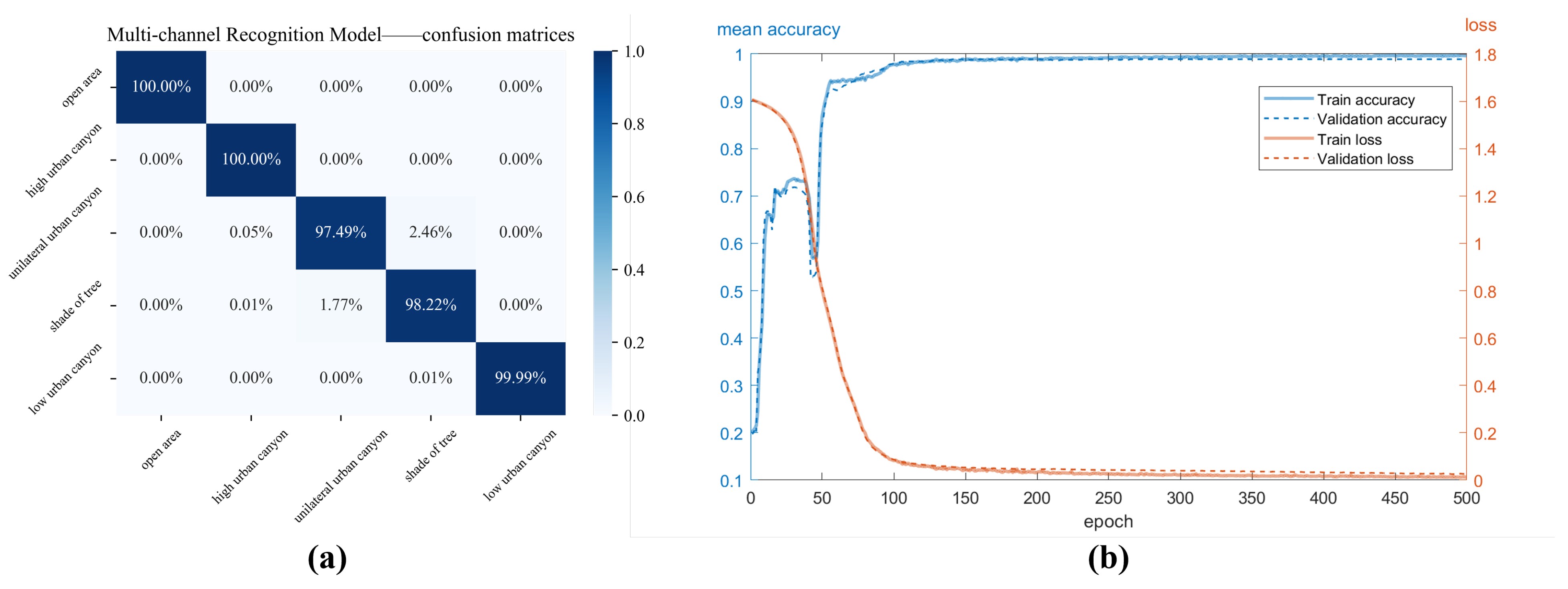
A spatio-temporal correlated method for constructing raw data features is used to analyze the importance of different observation data in recognition based on machine learning. A multi-channel Long Short-Term Memory (MC-LSTM) network for GNSS scene recognition is proposed. The result shows that our method can achieve an accuracy of 99.14% under the condition of using low-cost GNSS receivers to observe single satellite navigation system.

(c)

In order to manage the degradation in performances between different time periods, we conduct the transfer learning test of our method’s model. The result shows that our pre-trained model can be fine-tuned with a small number of epochs to adapt to different time periods at the same location, which is cost-acceptable for bike-sharing operators.

The remainder of this article is organized as follows: Section 2 introduces the methodology of our proposed model. Section 3 presents the experiments and an analysis of the results. Section 5 provides our conclusions and directions for future works.

2. Methodology

In this section, we first present the feature analysis and construction. Then we propose a deep-learning-based scene recognition model. The overview of our model is shown in Figure 1. The observation data are firstly constructed into different feature vectors. Then those feature vectors are fed into a multi-channel long short-term memory network (MC-LSTM) to identify five scenes (open area, high urban canyon, unilateral urban canyon, shade of tree, low urban canyon).

2.1. Feature Analysis and Constructions

In this subsection, we first present the observation data and their hidden information. Then we introduce the elevation and azimuth, which shows the geometric relationship between navigation satellites and receivers. Finally, we propose the feature vector definition for our model’s input.

2.1.1. GNSS Observations

Global Navigation Satellite Systems (GNSS) typically consist of three segments: the space (space navigation constellation and satellites), the ground control (master control station, monitoring stations and uploading stations), and the user terminals. Users can receive carrier signals transmitted by the space satellites by various of terminals (receivers). The carrier signals are modulated with ranging codes and navigation messages which can be processed by receivers into different observation data, including the Pseudo range [23], Carrier Phase [24], Doppler frequency [25] and $C/N_0$ [26].

Pseudo range: The pseudo range observation is an absolute measurement of the distance from the satellite to the receiver, obtained by measuring the signal propagation time delay, and is expressed in meters. The pseudo range includes atmospheric delays and clock biases, and its accuracy is typically at the meter level.

Carrier Phase: Carrier phase observations measure the phase difference between the satellite carrier signal and the reference carrier signal produced by the receiver’s oscillator, making it a relative observation. It is expressed in cycles and includes atmospheric delays, clock biases and ambiguity of whole cycles.

Doppler frequency: The frequency of the GNSS carrier signal received by the receiver differs from the actual frequency transmitted by the satellite. This difference is known as the Doppler shift, and its magnitude is related to the rate of change in distance between the receiver and the satellite. Specifically, the Doppler observation equation for GNSS is as follows:

$$\lambda D_r^s=\dot{{\rho }_r^s}-\left(\dot{\delta t_r}-\dot{\delta t^s}\right)c-\dot{{\delta }_{ion}^s}+\dot{{\delta }_{trop}^s}$$

(1)

where $D_r^s$ is the Doppler frequency and it is expressed in Hz. $\lambda$ is the wavelength of the carrier wave. $\dot{{\rho }_r^s}$ is the rate of change of the distance between the receiver (subscript r denotes the receiver) and the satellite (superscript denotes the satellite). $\dot{\delta t^s}$ and $\dot{\delta t^s}$ is the clock drift of the receiver and the satellite. $\dot{{\delta }_{ion}^s}$ and $\dot{{\delta }_{trop}^s}$ is the time derivatives of ionospheric and tropospheric delays.

C/N₀: The carrier-to-noise density ratio (or $C{N}_0$ in more straightforward terms) refers to the ratio of the signal power to the noise power per unit bandwidth in the received GNSS signal. It is expressed in dB and reflects the quality of the RF signal received by the receiver.

Then we consider the characteristics of above observations in urban static positioning scene. Under the conditions of no signal occlusion, the distance between the receiver and the satellite changes in a predictable manner due to the receiver being stationary and the satellite moving in a fixed orbit. In different obstruction scenes, the nature of the obstructions and the characteristics of multipath reflections cause varying rates of change in the distance between the receiver and the satellite. Therefore, we believe that the temporal characteristics of the observations can serve as a basis for scene recognition.

All these observation data can be read directly from Receiver Independent Exchange Format (RINEX format) files or the receivers’ output data stream without additional calculations. This is favorable for our application scene which only supports edge computing power. In order to unify the data scale, we normalize the raw observations as follows:

$$d_{norm}={\displaystyle \frac{d-d_{min}}{d_{max}-d_{min}}}$$

(2)

where $d_{max}$ and $d_{min}$ are the maximum and minimum values of a specific type of observation data within a time step, and d is the original observation data. The normalization only requires simple arithmetic operations, but can ensure network convergence [27,28].

2.1.2. Satellite Elevation and Azimuth

The satellite elevation angle refers to the angle between the vector from the user’s location to the satellite’s position and its projection onto the Earth ellipsoid tangent plane passing through the user’s location. The satellite azimuth angle refers to the angle between this projection and the true North coordinate axis on the tangent plane, with counterclockwise direction considered positive. The satellite elevation angle and azimuth angle are both related to the position of the user’s receiver [29]. They reflect certain aspects of satellite signals, ranging accuracy, and multipath effects. As shown in Figure 2, visible satellites often exhibit different geometric distributions under various obstruction scenes. The calculation methods for satellite elevation angle and azimuth angle are as follows [30]:

$$\left[\begin{array}{c}{N}_{zs}\\ E_{zs}\\ U_{zs}\end{array}\right]=H\times \left[\begin{array}{c}{X}_{es}-X_p\\ Y_{es}-Y_p\\ Z_{es}-Z_p\end{array}\right],H=\left[\begin{array}{ccc}-sin{B}_{p}cos{L}_p& -sin{B}_{p}sin{L}_p& cos{B}_p\\ -sin{L}_p& cos{L}_p& 0\\ cos{B}_{p}cos{L}_p& cos{B}_{p}sin{L}_p& sin{B}_p\end{array}\right]$$

(3)

where $N_{zs}$, $E_{zs}$, $U_{zs}$ represent the satellite position in the local topocentric coordinate system (ENU). $X_{es}$, $Y_{es}$, $Z_{es}$ and $X_p$, $Y_p$, $Z_p$ represent the satellite position (calculated from the satellite ephemeris) and station position in the Earth-Centered Earth-Fixed coordinate system (ECEF), respectively. H is the transformation matrix between ENU system and the ECEF system. $B_p$ and $L_p$ are the geodetic latitude and longitude of the receiver. Therefore, the elevation ($El$.) and azimuth ($Az$.) angle is calculated as follows:

$$Az=arctan\left({\displaystyle \frac{E_{zs}}{N_{zs}}}\right),El=arcsin\left({\displaystyle \frac{U_{zs}}{\sqrt{E_{zs}^2+N_{zs}^2+U_{zs}^2}}}\right)$$

(4)

From the physical definitions of the satellite elevation angle and azimuth angle, it can be observed that both the elevation and azimuth angles have upper and lower bounds. The elevation angle ranges from 0 to 90 degrees, and the azimuth angle ranges from $-180$ degrees to 180 degrees. Similarly to the normalization method used for raw observations, we normalize the satellite elevation and azimuth angles as follows:

$$A{z}_{norm}={\displaystyle \frac{Az-(-180)}{180-(-180)}},E{l}_{norm}={\displaystyle \frac{El-0}{90-0}}$$

(5)

where the elevation and azimuth angles are both expressed in degree.

2.1.3. Feature Vector Definition

The feature vector is used as the input of recognition model. In this subsection, we are going to introduce our feature vector definition, which considers both original observation data and geometric relationships between satellites and receivers. We use fixed-length sequential vectors to represent the constellation of a specific satellite navigation system. For example, a 32-dimensional vector is used to store the normalized pseudo range observations of GPS because the pseudo-random noise (PRN) code of satellites is in range of 1 to 32 (G01∼G32).

Additionally, we regard the satellite elevation and azimuth angles as a combined feature, which represents the geometric distribution of satellites that the receiver can use. Instead of changing visible satellites into sky plots like Figure 2, we use a $2N$-dimensional vector to store the normalized angles(where N is the max PRN of the navigation satellite system). Actually, the different dimensions of observation data is the basic of establishment of our multi-channel model, which will be introduced in Section 3 in detail. Our feature definition can be summarized as

Table 1. Brief Feature Definition List.

Feature Information	Feature Dimension
Elevation and azimuth angles	2N 1
Pseudo range	N
Carrier phase	N
Carrier phase and LLI	$2N$
Doppler frequency	N
$C/N_0$	N

¹ Where N is the max number of PRN for the navigation satellite system. For example, if the satellite system is GPS, $N=32$.

. It is worth noting that these vectors of different dimensions can be used both individually and in combination as the input of the multi-channel model.

2.2. A Multi-Channel Model for Scene Recognition

In this subsection, we first introduce the Long Short-Term Memory (LSTM) model, which is served as the fundamental building block for the construction of our model. After comparing the performances of different channels (different feature vectors), we propose our multi-channel model to integrate information from different channels. Finally, we consider the transferability of the model and introduce the transfer learning strategy we use in the temporal dimension.

2.2.1. LSTM and Single-Channel Network

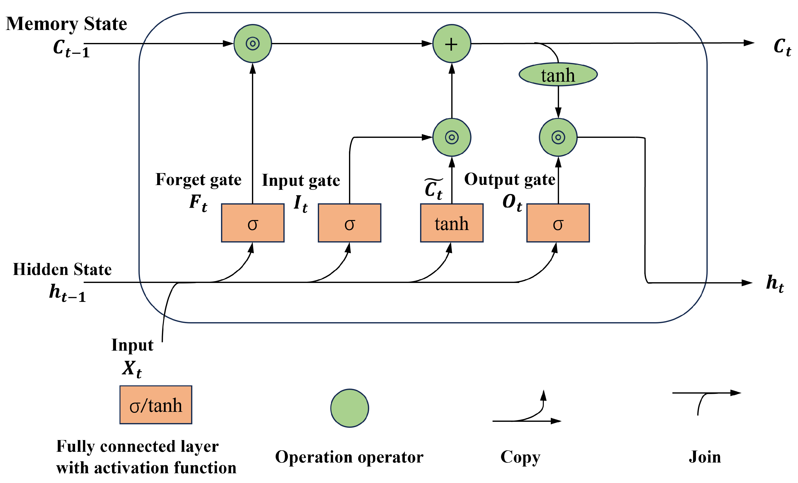
Long short-term memory (LSTM) networks are primarily used for learning and predicting temporal features in data sequences. Actually, in the field of GNSS positioning scene recognition, LSTM has been proven to be the most effective network model among numerous machine learning models [21,22,31]. LSTM is composed of numerous LSTM cells Figure 3, which are used to determine whether information is useful. There are three gates in one cell, including a input gate, a forget gate and an output gate. Additionally, a candidate memory cell is set in the LSTM cell in order to process the chosen memory. A hidden state $h_{t-1}$ and the memory passed to the next cell $C_t$ are output by each cell. The key expression of the LSTM cell is as follows [32,33,34]:

$$I_t=\sigma (X_t{W}_{xi}+h_{t-1}{W}_{hi}+b_i)$$

(6)

$$F_t=\sigma (X_t{W}_{xf}+h_{t-1}{W}_{hf}+b_f)$$

(7)

$$O_t=\sigma (X_t{W}_{xo}+h_{t-1}{W}_{ho}+b_o)$$

(8)

$$\widehat{C_t}=tanh(X_t{W}_{xc}+h_{t-1}{W}_{hc}+b_c)$$

(9)

$$C_t=F_t\odot C_{t-1}+I_t\odot \widehat{C_t};$$

(10)

where ⊙ represents the dot product and $\sigma$ represents the sigmoid activation function. $I_t$, $F_t$, $O_t$ are the outputs of the input gate, forget gate and output gate. $W_{xi}$, $W_{h}i$; $W_{xf}$, $W_{hf}$; $W_{xo}$, $W_{ho}$ are the weight matrices of input, forget, output gates. $W_{xc}$, $W_{hc}$ are the weight matrices of the candidate memory cell. $b_i$, $b_f$, $b_o$, $b_c$ are the biases. The hidden state $h_t$ is caculated as follows:

$$h_t=O_t\odot tanh\left(C_t\right)$$

(11)

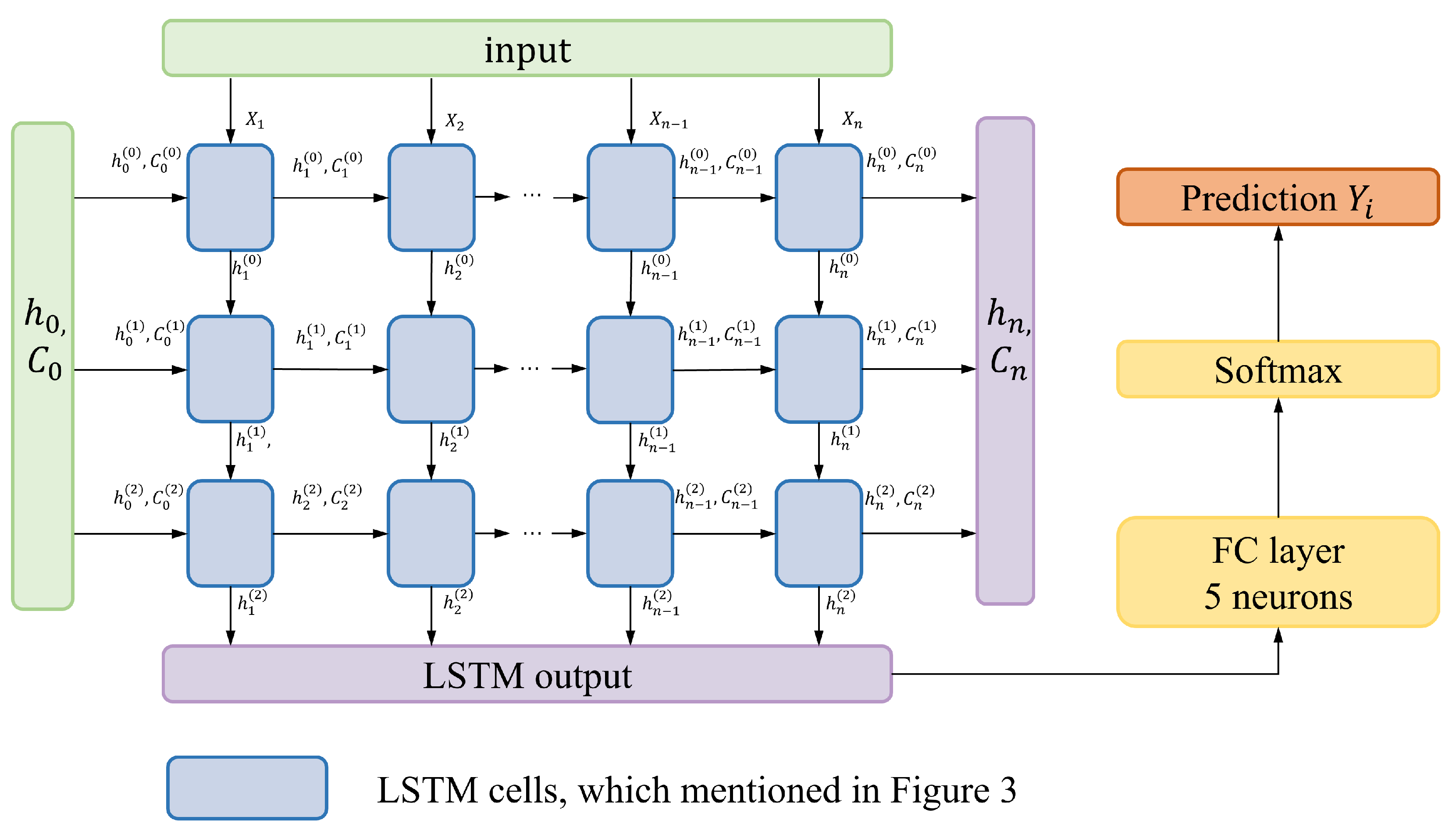
To change our feature vector to the input of LSTM, the original feature vector sequences should be transmitted into time segments with a sliding window. It means we combine data vectors within a certain time step into a sequence in chronological order and make it the input of single channel. Take pseudo range feature for example, if a N-dimensional vector represents the normalized pseudo range of the time $t_0$, the input of single LSTM channel is in dimension of $(t_s,N)$, where $t_s$ is the time step of sequence. The overview of our single channel LSTM is shown in Figure 4.

To ensure the real-time performance of the algorithm and consider the practical application requirements, we add only 3 LSTM layers in a single channel which is used to process a single type of feature vector. Meanwhile, the time step is set in 10 s. The sliding window is set in 1 s so that 2990 sequences of each scene can be collected. Similar to the majority of machine learning classification tasks, we use the cross-entropy loss function and optimize the parameters of the network with Adam. The network is trained on training and validation datasets for approximately 500 epochs. The batch size is set to 32 and the learning rate is set to $0.00001$.

2.2.2. Scene Categories and Single Channel LSTM Performances

Usually, GNSS positioning scenes are divided into two main parts: outdoor and indoor [17,18,19]. Within urban environments, urban canyons and boulevard are also considered in scene recognition [22,35]. Given the specificity of our application scene (static positioning for shared bikes’ parking), we have subdivided urban canyons into high urban canyon, low urban canyon and unilateral urban canyon. So we divide the positioning scenes into five categories: open area, shade of tree, high urban canyon, low urban canyon and unilateral urban canyon. Due to the bike parking rule, we no longer consider the indoor scenes, which are easily identifiable based on the presence of satellite signals. Figure 5 shows the real-world locations and the street view where we collected data, and Figure 2 shows the distribution of satellites in various scenes.

In our proposed algorithm, we encode the scene categories as one-hot vectors as

Table 2. Scene Categories and Encoding.

Categories	Encoding
open area	[1, 0, 0, 0, 0]
high urban canyon	[0, 1, 0, 0, 0]
unilateral urban canyon	[0, 0, 1, 0, 0]
shade of tree	[0, 0, 0, 1, 0]
low urban canyon	[0, 0, 0, 0, 1]

. So the index of the max number of output vector represents the highest possibility of the scene. For example, if the model outputs a vector of [0.1, 0.1, 0.5, 0.2, 0.1], the prediction result of scene recognition is the unilateral urban canyon. Under the training setting mentioned in subsection, we have trained and validated the single channel model and the performances are shown in Figure 6.

From the confusion matrices shown in Figure 6, we can find that different feature data have varying sensitivities to the recognition of different scenes. The feature of az/el and $C/N_0$ performs the best in all categories while other feature data performs in specific category (pseudo range in shade of tree, phase + LLI in high urban canyon). Meanwhile, the convergence speeds of the individual single-channel models also show significant differences, as shown in Figure 7. The az/el has the fast convergence speed while the phase has the slowest. Moreover, the performance of phase + LLI is better than single phase no matter the accuracy or the convergence speed, which prompts us to combine the carrier phase and LLI into one feature consideration in the subsequent research.

2.2.3. MC-LSTM Design

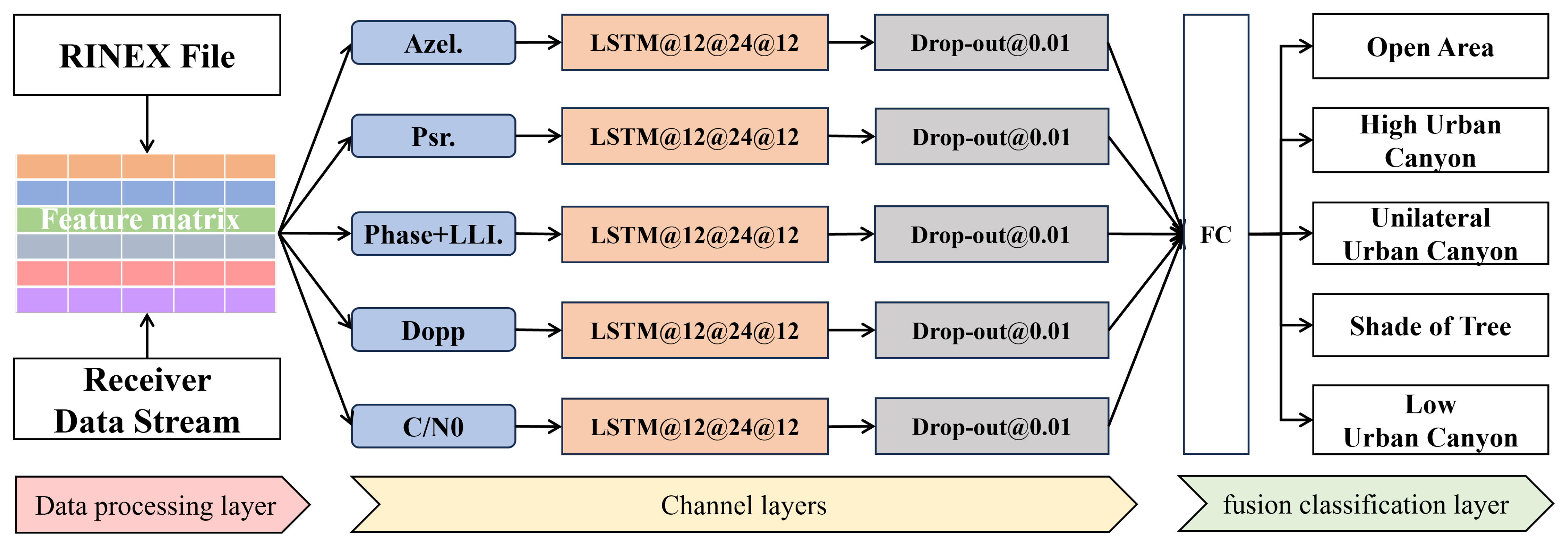
In the last subsection, we analysed the performances of different feature vectors. To improve recognition accuracy and convergence speed of our model across all scenes, we integrate information from different feature vectors through a multi-channel parallel design. The overview of our model is shown in Figure 8. The model consists of channel layers and a fusion classification layer. Different feature vectors are input into corresponding LSTM channels. After LSTM processes and outputs hidden states, these are passed through fully connected layers to merge and classify scene recognition results. It is important to note that the dropout layers are used to introduce non-linearity to the model, which helps prevent overfitting and enhances the model’s ability to generalize [36,37].

In addition, our proposed multi-channel model allows for flexible combinations of channels based on scenes and requirements. If the receiver cannot output a certain type of observation, the corresponding data vector channel can be excluded.

2.2.4. Transfer Learning Settings

A trained model can achieve a high accuracy in training and validation dataset but usually does not perform well in another dataset. Therefore, classification models need to be retrained when changes in the feature space or the feature distribution occur [38]. In our application scene for recognizing shared bicycle parking locations, the absolute position used is generally fixed, but the time when users park is random. It makes the cost exceptionally high for collecting data from all time periods for training. Therefore, the quicker we can execute the transfer learning between time periods, the stronger our model’s generalization is. This means the operator of shared bikes can quickly deploy the pre-trained model with simple fine-tuning to different time periods, significantly reducing the time required for model training. To test the temporal transfer performance of our model, we collected data from different time periods and performed full-layer transfer. The distribution of the data over time is shown in

Table 3. Transfer Learning Data.

Dataset	Scene	Time of First Observation	Lasting Time
Dataset-1	open area	10:31/13:04/14:16/15:21/16:26	10 min for each
	high urban canyon	10:43/13:16/14:28/15:32/16:38	10 min for each
	unilateral urban canyon	10:57/13:33/14:40/15:45/16:51	10 min for each
	shade of tree	11:16/13:44/14:55/16:00/17:15	10 min for each
	low urban canyon	11:34/14:02/15:07/16:13/17:28	10 min for each
Dataset-2 *	open area	11:09	10 min
	high urban canyon	11:21	10 min
	unilateral urban canyon	11:33	10 min
	shade of tree	11:44	10 min
	low urban canyon	11:57	10 min

* The dataset which is used as the target of transfer learning.

.

3. Results

In this section, we first introduce the device we used and the dataset we collected. We then analyze the performance of our model and compare it with those from other studies. Finally, we evaluate the real-time performance of our proposed model and present the transfer learning results.

3.1. Device and Dataset

The experimental data were collected using a receiver based on HD8020 series chipset (Allystar Technology, Shenzhen, China), which is a low-cost GNSS receiver chip solution widely used in shared bikes. The appearance of the data collection device is shown in Figure 9. In order to closely replicate the shared bicycle parking scene, we chose not to alter the structure of the bike’s positioning system (GNSS module + antenna). Instead, we directly connected the bike’s built-in module to a PC via a serial port to obtain data.

To ensure the generalization performance of our proposed model, During each time periods, we collected 10 min’s data for each positioning scene (open area, high urban canyon, unilateral urban canyon, shade of tree and low urban canyon). Five such time periods are taken into consideration. Moreover, We shuffled the collected data samples before training and used a cross-validation strategy (70% for training while 30% for validation). As for the dataset for time-transfer-learning, we collected the same distribution data a few days later than training data. The total distribution of the dataset is shown in Table 3.

3.2. Multi-Channel LSTM Model Results

In this subsection, we analyze the performances of our proposed model. First, we introduce the recognition accuracy of our multi-channel LSTM model by confusion matrices and show the changes of accuracy and loss through training epochs by figure. We then compare the results (including accuracy and convergence speeds) of multi-channel model and single channel LSTM mentioned in Section 3. Finally, we compare the performances of our model and other proposed algorithms in recent years.

The confusion matrices and loss and accuracy changes in training epochs are shown in Figure 10. Our model can reach a mean accuracy of 99.14% in all categories and an accuracy of at least 97.5% for each individual category on validation set. From the loss & accuracy changes we can easily find that after only a few training epochs (about 50 epochs) our model is already reaching an accuracy over 90%, which shows it performs well both in recognition as well as training consumption. We observed that the training and validation accuracy of the model initially dropped once during the training process and then quickly increased. This indicates that adding dropout layers in the single channel helps prevent the model from getting stuck in local optima, which aligns with our understanding of nonlinear models [39].

Now we are going to take multi-channel and single-channel into consideration. Compared with the single-channel model mentioned in Section 3, the multi-channel can reach higher accuracy in scene recognition, including mean accuracy of all categories as well as the specific category. The detailed comparison is shown in

Table 4. Comparison between Multi-Channel and Single-Channel.

Channel *	Accuracy in Scenes					Mean Accuracy
	Open Area	High Urban Canyon	Unilateral Urban Canyon	Shade of Tree	Low Urban Canyon
azel	97.31%	94.16%	92.53%	91.76%	98.77%	94.90%
psr	69.47%	86.47%	87.95%	96.03%	98.00%	87.58%
adr	99.60%	90.61%	85.33%	78.91%	98.55%	90.60%
adrs	99.80%	98.86%	91.55%	80.74%	95.71%	93.22%
dopp	94.79%	80.96%	44.92%	88.46%	96.50%	81.13%
$C/N_0$	98.44%	99.60%	94.73%	93.01%	96.71%	96.50%
Multi-channel	100.00%	100.00%	97.49%	98.22%	99.99%	99.14%

* Where “azel” represents the azimuth and elevation angles, “psr” represents the pseudo range, “adr” represents the carrier phase, “adrs” represents the carrier phase plus LLI (loss of lock indicator), “dopp” represents the doppler frequency. “multi-channel” represents our proposed recognition model: MC-LSTM.

.

Despite the accuracy, convergence speed is also an important metric for evaluating model performance. Compared with the single channel model, be similar to accuracy, multi-channel model can also converge faster. Take azimuth and elevation angles channel (the fastest channel in convergence speed) for example, just like Figure 11 shows, the multi-channel model is faster than any other single channel in convergence speed. All results above indicate that our multi-channel design significantly enhances the performance of LSTM in recognizing GNSS positioning scenes, in terms of both accuracy and convergence speed. This demonstrates the benefits of our strategy to integrate multiple channels. It is worth noting that instead directly using existing network, our proposed model design strategy is one of the few specialized network structures specifically designed for GNSS positioning scenes in current related research.

After analyzing the accuracy and convergence speeds, we have already substantiated that our model exhibits superior performance in GNSS positioning scenes recognition.

Table 5. Scene Categories and Encoding.

Authors	Years	Methods	Scenes *	Accuracy
Chen et al. [17]	2017	Threshold judgment	I/O	85.6%
Wang et al. [35]	2019	SVM & temporal filtering	5 urban dynamic scenes	89.30%
Lai et al. [20]	2021	SVM	3 scenes of I/O	90.3%
Dai et al. [21]	2022	CNN & conv-LSTM	4 scenes in I/O	98.82% & 99.92%
Zhu et al. [22]	2024	LSTM	4 urban dynamic scenes	95.39%
Ours	2024	MC-LSTM	5 urban static scenes	99.14%

* Where the scenes that GNSS signals can not be received is ignored in this table. I/O means the indoor and outdoor scenes.

shows the comparison between our model and other proposed algorithms in recent years, including accuracy and scene granularity. Our model is the only algorithm which can achieve an accuracy of 99% across five scenes (the scene no GNSS signal received is not included). Indeed, we are also the only researchers who take detailed urban scenes (high, low and unilateral) into consideration.

3.3. Potential Real-Time Ability

In this subsection, we analyze the real-time ability of our proposed model, including the consumption of offline model-training and online model-prediction. We randomly selected 3000 s (2950 time sequences are constructed) of data from the training dataset to evaluate the real-time performance of our model. It is noteworthy that we chose a CPU (Intel (R) Core (TM) i5-12500H, 2.5 GHz) but not a GPU as the computing platform for our real-time performance test and still achieved excellent results.

To evaluate the time consumption of model-training and model-prediction, we first introduce the definition of the metrics: training time per epoch (TPE) and prediction time per data (PPD). Our TPE and PPD is shown in Figure 12. 0.75 s is cost the most in training a dataset of 2950 sequences for one epoch, which makes it possible for our model to do the online fine-tune according to the real-time data. Moreover, only 1.95 ms is needed to perform a full prediction, which makes it possible for our model to be deployed in real-time scenes without any noticeable additional time delay. Compared with existing convolution blocks-relied works, our specially designed multichannel model has a 60% improvement in TPE and 90% in PDD [21,22]. Only 40,817 parameters are included in our model.

3.4. Time-Transfer Ability

The high precision a pre-trained model can achieve requires that the training data and the test data have similar distributions in feature spaces. Therefore, classification models need to be retrained when changes in the feature space or the feature distribution occur [38]. In our application scenes, we always face that the cost of collecting data of all time periods is unacceptable. Meanwhile, the temporal dimension is a decisive factor in evaluating the generalization capability of our model. So the transfer ability between time periods is taken into consideration in our model.

Table 6. Comparison between transfer and non-transfer learning.

Scenes *	Accuracy through Epochs
	0 Epoch		10 Epochs		20 Epochs		30 Epochs		100 Epochs
	T.	Non-T.	T.	Non-T.	T.	Non-T.	T.	Non-T.	T.	Non-T.
open a.	98.31%	19.84%	100.00%	0.00%	100.00%	85.59%	100.00%	0.00%	100.00%	99.83%
high u.c.	3.39%	19.85%	90.85%	55.76%	94.92%	98.64%	97.63%	100.00%	99.32%	100.00%
unilateral	0.00%	19.68%	98.81%	0.00%	100.00%	0.00%	96.27%	3.90%	96.27%	88.81%
s.o.t.	0.00%	19.97%	0.00%	19.32%	6.61%	88.81%	100.00%	91.53%	100.00%	100.00%
low u.c.	85.93%	20.58%	88.47%	100.00%	95.76%	100.00%	95.93%	99.66%	100.00%	98.64%
mean	37.52%	19.98%	75.62%	35.02%	79.46%	74.61%	97.97%	59.02%	99.12%	97.46%

* Where “open a.” represents the open area, “high u.c.” represents the high urban canyon, “unilateral” represents the unilateral urban canyon, “s.o.t.” represents the shade of tree, “low u.c.” represents the low urban canyon. Columns named “T.” shows the transfer learning results while “Non-T.” shows the non-transfer learning.

shows the details of transfer learning and we can find that our pre-trained model can be fine-tuned with a small number of epochs to adapt to different time periods at the same location. Moreover, the transfer learning performs better than non-transfer (directly) learning in most scenes and training stages. The mean accuracy of transfer learning at every check points (0, 10, 20, 30 and 100 epochs) is higher than non-transfer learning.

3.5. Data-Loss Robustness

Due to the limitations in the number of observation channels of low-cost receivers, the application of our model always faces the situation that some observation data are missing. Therefore, we decide to do an additional experiment to evaluate the robustness of our model in such data-missing situations. As the azimuth and elevation angles are calculated by satellite ephemeris and receiver’s position, the pseudo range is the least requirements of calculating the azimuth and elevation angles. So we divide the channels into four groups to test our model’s robustness: pseudo range and azimuth & elevation angles (G1), carrier phase and LLI (G2), Doppler frequency (G3), $C/N_0$ (G4). As the results show in

Table 7. Channel-missing Robustness.

Combinations	Mean Accuracy
G1 & G2	54.80%
G1 & G3	81.13%
G1 & G4	54.24 %
G1 & G2 & G3	90.28%
G1 & G2 & G4	57.17%
G1 & G3 & G4	96.06%

, our model can achieve an accuracy of over 80% even in the situation that one or two channels’ missing. For example, if the carrier phase data and $C/N_0$ data are missing, our model can also reach an accuracy of 81.13% in scenes recognition.

4. Discussion

4.1. Detailed Scenes Recognition in Urban Static GNSS Positioning

Accurate GNSS scenes recognition in urban environments plays an important role in high-precision urban positioning. All the scene-adaptive methods to improve the precision of GNSS positioning require efficient scenes recognition. As shown in Table 5, existing works mainly focus on Indoor and Outdoor recognition [17,20,21] or only consider coarse-grained outdoor scenes [22,35]. Especially for the urban canyon, most research has ignored the different directions of signal blockage. Our proposed model considers the real requirements of urban static positioning application (shared bike parking) and divides the urban canyon scene into high, low and unilateral categories. It achieves an accuracy of over 99% in scenes recognition and is specially designed in multi-channel structure according to the characteristics of GNSS tasks, which represents great progress compared with directly using the existing networks in this field. Detailed scenes and multi-channel network structure design provide a new perspective of GNSS scenes recognition and has the possibility of freely adapting to different tasks according to environments.

4.2. Potential in Real GNSS Scenes Recognition Application

The complexity of urban environment and the limitation of computing power of equipment have always been the main obstacles to the practical application of GNSS scene recognition method based on deep learning. The lightweight network parameter scale, real-time ability and robustness to signal reception failure should be taken into consideration in the real GNSS scenes recognition application. Existing works achieve high precision of recognition by using convolution blocks, which makes the scale of network parameters unacceptable for low-cost computing devices. Our proposed model lightened the hidden layers according to the characteristics of GNSS features and only requires milliseconds of extra time in recognition. Surprisingly, our multi-channel model can also achieve high recognition accuracy even in cases where some observations are lost. All the above findings show that our proposed multi-channel LSTM network structure has a wide potential in real GNSS scenes recognition applications.

5. Conclusions

In this study, a scenes recognition model for urban static GNSS positioning is proposed. The proposed model is able to provide detailed scene information only using a single satellite system’s observations via low-cost receivers equipped on the shared bikes. It organizes the original observation data into five feature vectors with different dimensions but without any additional calculation except normalization. After analyzing the performances of different feature vectors, a specially designed multi-channel LSTM model is proposed to further improve the recognition accuracy in different scenes. Experiments are designed to evaluate the proposed model in terms of accuracy, time consumption and robustness. The results show that our proposed model can achieve an average accuracy of 99.14% in all scenes and at least 97.5% in an individual scene. The time delays of model training and prediction on a CPU are 0.75 s per epoch and 1.95 ms per data, which makes it possible for our model to be deployed in real-time applications. Furthermore, our model can be transferred into different time periods with only a few epochs training and maintain a high accuracy even in the presence of missing channel data (96.06% for one channel missed and 81.13% for two channels missed), which shows the robustness of our model in real-world applications. In future works, more detailed and mixed scenes should be taken into consideration. In addition, the contributions from different satellite systems and frequencies require further research.