An Ambient Adaptive Global Navigation Satellite System Total Electron Content Predictive Model for Short-Term Rapid Geomagnetic Storm Events

Abstract

Satellite navigation is an essential component of the national infrastructure. Space weather and ionospheric conditions are the prime sources of GNSS (global navigation satellite system) positioning, navigation, and timing (PNT) service disruptions and degradations. Protection, toughening, and augmentation (PTA) of GNSS PNT services require novel approaches in ionospheric effects mitigation. Standard global ionospheric correction models fail in the mitigation of high-dynamics and local ionospheric disturbances. Here, we demonstrate that in the case of the short-term fast-developing geomagnetic storm, a machine learning-based environment-aware GNSS ionospheric correction model for sub-equatorial regions may provide a substantial improvement over the existing global Klobuchar model, considered a benchmark. The proposed machine learning-based model utilises just the geomagnetic field density component observations as a predictor to estimate TEC/GNSS ionospheric delay as the prediction model target. Further research is needed to refine the methodology of machine learning model development selection and validation and to establish an architecture-agnostic framework for GNSS PTA development.

1. Introduction

Standard GNSS (global navigation satellite system) ionospheric delay correction models suffer from shortcomings caused by their global nature and coverage, and constraints of the broadcast model parameters update on a daily basis. In such a manner, the standard GNSS ionospheric correction models, such as the Klobuchar model [1], used for GPS positioning, fail to account for local and sudden ionospheric events. Failure in the characterisation of the actual TEC propagates into GNSS pseudorange measurement errors, resulting in increased GNSS position estimation errors, and the delay affects the growing number of GNSS-based technology and socio-economic applications, as modern civilisation becomes reliant on GNSS positioning, navigation and timing (PNT) services and their guaranteed performance levels [2,3].

The ionospheric delay results from the conditions the satellite radio wave encounters during its propagation through the Earth’s ionosphere [4]. The impact propagation process that leads to the formation of the ionospheric delay, and, consequently, the GNSS pseudorange measurement errors and GNSS position estimation errors, was described with the Space weather–GNSS positioning performance coupling model [5].

The analytical expression of the ionospheric delay may be derived from the Appleton–Hartree equation [4]. Derivation yields the relation between the ionospheric delay Δt_iono [s] and the vertical ionospheric profile N(h) [electrons/m³], an analytical model of the free-electron density at a given height h above the Earth’s mean sea level, as given in (1). Physical constants used in (1) denote, as follows, e, unit electron charge (1.6 × 10⁻¹⁹ C); m_e, unit electron mass (9.1 × 10⁻³¹ kg); c, velocity of light in vacuum (2.99792458 × 10⁸ m/s); ε₀, permittivity of vacuum (8.854 × 10⁻¹² F/m); and ω, angular wave frequency in [rad/s]. Integration bounds in (1) are determined with the lower h_lower and upper h_upper boundary of the ionosphere.

$$\Delta t_{iono}={\displaystyle \frac{e^2}{2{ϵ}_0{m}_e{\omega }^{2}c}}{\int }_{h_{lower}}^{h_{upper}}N\left(h\right)dh$$

(1)

The introduction of numerical values of physical constants yields a relationship between the ionospheric delay of a radio signal and the vertical ionospheric profile, as expressed with (2) [4], with Δt_iono [s] denoting the ionospheric time delay, N(h) [electrons/m³] denoting the vertical ionospheric profile, h [m] denoting height above the mean sea level, c denoting the velocity of light in vacuum (2.99792458 × 10⁸ m/s) and f denoting radio carrier frequency.

$$\Delta t_{iono}={\displaystyle \frac{40.3}{c{f}^2}}{\int }_{h_{lower}}^{h_{upper}}N\left(h\right)dh$$

(2)

Satellite navigation systems operate under the presumption of satellite signal propagation at the velocity of light in vacuum along its path from a satellite aerial to a receiver aerial, a condition that is not met during the passage through the ionosphere and troposphere [6].

Multiplication of both sides of (2) with the velocity of light in vacuum c will yield an equivalent expression, describing the relationship between the error of the measured distance between a satellite and a receiver aerial $\Delta {\rho }_{iono}$ [m], the so-called pseudorange and the vertical ionospheric profile N(h), as given in (3) [2,7,8].

$$\Delta {\rho }_{iono}={\displaystyle \frac{40.3}{f^2}}{\int }_{h_{lower}}^{h_{upper}}N\left(h\right)dh={\displaystyle \frac{40.3}{f^2}}TEC$$

(3)

The integral factor in Equations (1) and (3) is known as Total Electron Content (TEC). TEC, expressed in [electrons/m²], denotes the surface density of free electrons encountered by a satellite radio signal traveling along its path. TEC takes large values and is commonly expressed in TECU units (1 TECU = 1 × 10¹⁶ electrons/m²). TEC results from the ionospheric conditions described with the vertical ionospheric profile N(h), which renders TEC the outcome of the ionospheric conditions, rather than the ionospheric descriptor.

The unmet presumption of the satellite radio signal propagation at the constant velocity of light in vacuum is the prime single cause of the satellite positioning error [6]. Ionospheric conditions cause a complex behaviour of the GNSS ionospheric delay, described with a bias and random error components [5]. Quiet space weather, geomagnetic and ionospheric conditions render the bias component of the ionospheric delay dominant, while in disturbed ionospheric conditions, the influence of the random component dominates. Standard ionospheric delay correction models, such as the Klobuchar model for GPS, Beidou and Glonass (CDMA) systems, address the bias component of the GNSS ionospheric delay. This causes minor to considerable problems for the GNSS ionospheric delay prediction, and the resulting GNSS PNT degradation, in times of space weather, geomagnetic and ionospheric disturbances, as shown in Figure 1.

Sudden, localised and short-term geomagnetic and ionospheric disturbances are of particular concern, as such conditions are not described correctly with the standard correction models, which have a global nature and extent; do not consider local disturbances; and have the correction model parameters updated rarely (once a day) [5,6].

Ionospheric delay may be mitigated successfully using simultaneous pseudorange measurements at two different carrier frequencies [6]. The dual-frequency method is commonly applied in specially authorised GNSS positioning processes [2,7,8]. However, the vast majority of GNSS receivers on the market utilise a single-frequency approach. In an application of the reverse-engineering process, the dual-frequency method may be utilised for the determination of TEC.

Thus, a GNSS receiver becomes a TEC sensor [3,9]. It may be shown that the actual TEC encountered on the satellite signal path seen from the receiver perspective as coming at the elevation angle E [rad] may be determined using (4) [6], where the related symbols denote the following: STEC denotes slant (actually observed) TEC, at elevation angle E; $\rho \left(f_1\right)$ and $\rho \left(f_2\right)$ denote simultaneously observed (measured) pseudoranges in [m] at frequencies f₁, and f₂, respectively; b_s denotes satellite bias in [m]; and b_r denotes receiver bias in [m]. Various implementations of the TEC estimation procedure deploy different approaches in the estimation of satellite and receiver bias.

$$STEC={\displaystyle \frac{\rho \left(f_2\right)-\rho \left(f_1\right)-b_s-b_r}{40.31\cdot \left[\frac{1}{f_2^2}-\frac{1}{f_1^2}\right]}}$$

(4)

TEC observations should be normalised for satellite signals traveling different paths and distances, passing different segments of the Earth’s ionosphere. A mapping function m(E) was introduced to determine the normalised vertical TEC (VTEC) [2,6,8], as given in Equations (5) and (7), with R_Earth denoting the Earth’s radius and h denoting height above the mean sea level.

$$STEC=m\left(E\right)\cdot VTEC$$

(5)

$$m\left(E\right)={\displaystyle \frac{1}{\sqrt{1-{\left(\frac{R_{Earth}}{R_{Earth}+h}\cdot cos\left(E\right)\right)}^2}}}$$

(6)

$$TEC={\displaystyle \frac{\sqrt{1-{\left(\frac{R_{Earth}}{R_{Earth}+h}\cdot cos\left(E\right)\right)}^2}}{40.31}}\cdot {\displaystyle \frac{f_1^2{f}_2^2}{f_1^2-f_2^2}}\cdot \left[\rho \left(f_2\right)-\rho \left(f_1\right)-b_s-b_r\right]$$

(7)

Recent TEC prediction model developments for the purpose of GNSS position estimation improvement were focused on the traditional time-series techniques, with the utilisation of spherical harmonics for GNSS position estimation improvement [10,11]. Ref. [3] proposed the adaptive GNSS-based positioning process, which respects the actual state of the local environment for satellite positioning. Dubbed the ambient adaptive PNT, it exploits the abundance of precise sensors accompanying GNSS receivers, such as those in smartphones, which are capable of the GNSS PNT environment observation, as well as trusted detailed third-party data on the same subject. The adaptiveness to the GNSS PNT environment is based on the situation awareness obtained either using trusted third-party data for the region in question and/or direct measurements of descriptors of the GNSS PNT environment performed at the position of a GNSS receiver. Development of the adaptive GNSS-based positioning process involves the introduction of advanced position estimation methods [3], as well as observations-based and statistical learning-founded [12] prediction correction models. While statistical learning methods have been utilised in space weather research [13], their utilisation in satellite navigation for mitigation of the ionospheric effects is still novel [5,9,14].

Here, we contribute to the subject with a proposal for and a demonstration of a method for an ambient-aware tailored personalised GNSS ionospheric delay correction model development based on observations of the local geomagnetic environment (geomagnetic field density). The research aims at the provision of a reliable and robust GNSS TEC prediction model based on the current observations of the immediate ambient (positioning environment) conditions and utilisation of machine learning methods for the GNSS TEC predictive model development and operation. The proposal targets single-frequency commercial-grade GNSS receivers, a class of GNSS receivers prevailing on the market. Considering its intended cross-disciplinary adoption and self-sustainable personalised deployment, the method and the correction model are anticipated to extend model development and deployment characteristics, such as (i) accuracy and precision in terms of both the bias and the variance, (ii) conceptual simplicity, (iii) fast model development and (iv) high efficiency and low energy consumption for model development and deployment. The model development and deployment methods are to serve the increasing number of GNSS PNT processes implemented in mobile and stationary GNSS PNT applications, including smartphones, autonomous road vehicles, aircraft, vessels and Internet-of-Things (IoT) devices, with a wide range of computational capacity levels and available energy constraints. The proposed GNSS TEC prediction model aims at the provision of an alternative to the standard TEC correction models, such as the Klobuchar model, thus becoming an integral component of the GNSS PNT process and algorithm.

Integrated into the GNSS PNT process and algorithm [3], the GNSS pseudorange measurement error/TEC model aims at the provision of adaptiveness to the GNSS ambient (positioning environment) conditions and improved mitigation of the GNSS ionospheric delay, compared with the Klobuchar model set up as the reference (benchmark) model.

2. Methods and Materials

The GNSS ambient conditions in the immediate vicinity of a GNSS signal-collecting mobile unit determine the degradation level of the GNSS PNT performance [6,8,15]. The statement holds for both a traditional GNSS receiver and a mobile unit of a positioning-as-a-service system [3]. The research presented hypotheses that the near-real-time situation awareness of positioning environment conditions may significantly reduce positioning performance degradation due to both natural and artificial adversarial effects. Furthermore, it is argued here that a bespoke GNSS correction model based on the situation awareness of the positioning environment conditions may be developed, maintained and operated by the reception side of the GNSS system. The concept relies on the assumptions of (i) internet-based connectivity; (ii) a mobile unit equipped with appropriate sensing devices, such as magnetometers, to be utilised for the positioning environment condition assessment; and (iii) the computational capacity of mobile units. All three presumptions are fulfilled in mass-market devices, such as smartphones, automobiles or personal computers, and will be in a vast range of Internet-of-Things devices. The proposed method may be considered a valuable contribution to the protection, toughening and augmentation efforts of the core GNSS without the need for expensive and complicated infrastructure development.

The proposed GNSS TEC predictive model is aimed to serve the GNSS community, and those utilising single-frequency GNSS receivers in particular, through harvesting ambient condition awareness. Its purpose is to provide a valuable alternative to the standard GNSS ionospheric correction models by exploiting the sensing, computational and information resources available to a mobile unit (a GNSS receiver) during its operation.

The complexity of space weather, geomagnetic and ionospheric disturbances creates a range of effects on the GNSS PNT performance and its degradation. Statistical properties of variables describing both the ionospheric conditions and the GNSS PNT performance differ significantly in different scenarios of the ionospheric disturbances. Separate assessments of various scenarios of ionospheric disturbances and the GNSS PNT performance degradations are, therefore, required. This research focuses on short-term rapidly developing ionospheric disturbances, one of the extreme scenarios of ionospheric disturbances that causes unexpected, fast and significant GNSS PNT performance degradation.

This section details the proposal of the concept, method and model, as well as material (data) used in practical implementation for a proof-of-principle demonstration.

2.1. TEC/GNSS Ionospheric Delay Prediction Model Development

Statistical learning methods for prediction model development and real-time observations of geomagnetic conditions and GNSS pseudorange measurements are used in the candidate sub-equatorial short-term rapidly developing ionospheric storm TEC prediction model. The B_x, B_y and B_z components of the geomagnetic field density vector in [T] are considered predictors of the TEC prediction model. The TEC experimental values are derived from the raw GPS pseudorange observations, using the common methodology described in Section 1, Equation (7). TEC derivation using model (7) in Section 1 is selected in consideration of the computational capacity of the targeted market of single-frequency commercial-grade GNSS receivers, mobile devices containing them and positioning-as-a-service systems. The experimental TEC values are considered true values for the purpose of the GNSS TEC predictive model development. TEC is considered the outcome of the sub-equatorial short-term rapidly developing ionospheric storm TEC prediction model. The TEC prediction model development procedure is outlined in Figure 2.

The Disturbance Storm-Time (D_st) index, a geomagnetic condition descriptor, is considered a selector of short-term rapidly developing geomagnetic storm scenarios [4,16]. Geomagnetic field density component observations and raw dual-frequency GNSS pseudorange observations collected during the selected short-term and rapidly developing geomagnetic and ionospheric storms are aggregated into a single set of original observations. Raw dual-frequency GNSS pseudoranges are used for the derivation of experimental TEC values. The exploratory statistical analysis is performed on components of geomagnetic field density (predictors) and derived TEC (outcome) to determine their statistical models. Results of the exploratory statistical analysis are used in the selection of statistical learning methods for candidate TEC prediction model developments. Models developed are validated on the independent testing set of TEC and geomagnetic field density component observations. The performance of candidate models is compared mutually and with the performance of the standard Klobuchar model to identify the best performer to be pronounced the sub-equatorial short-term rapidly developing ionospheric storm TEC prediction model.

2.2. Statistical Learning-Based Model Development Methods

This research embraces the concept of statistical learning on experimental observations of related statistical variables [17,18] for the development of candidates of the sub-equatorial short-term rapidly developing ionospheric storm TEC prediction model. The results of exploratory statistical analysis of the aggregated set of predictors and outcome observations lead to the selection of two statistical learning methods for the development of candidates for the sub-equatorial short-term rapidly developing ionospheric storm TEC prediction model.

2.2.1. Boosted Generalised Additive Model (GAMB) Development Method

The boosted generalised additive model (GAMB) development method is a machine learning method based on the generalised additive model introduced by [17] and its boosting enhancement [18,19,20]. The method is aimed at modelling the non-linear and non-parametric relations between the target variable and predictors. The generalised additive model (GAM) method allows for modelling the non-linear and non-parametric relations between the expectation of the target variable y and predictors {x₁, x₂, …, x_n} by extending the concept of linear regression through the development of the smoothing function g(E(y)) of one or more predictors (8), based on the penalised regression approach [17], with E(y) denoting the expectation of y, β₀ denoting a constant and f() denoting a function.

$$g\left(E\left(y\right)\right)=g\left(y¯\right)={\beta }_o+\sum _{i=1}^n{f}_i\left(x_i\right)$$

(8)

The boosting principle contributes to model development in a sense similar to the random forest approach. Through the boosting process, the predictions of multiple additive models, trained on subsets of the original observations, are combined in the optimisation sense to yield the response of the GAMB model. The GAMB model benefits from the deployment of boosting in terms of a reduction in the bias and variance of individual/simple models, thus achieving improved accuracy and robustness.

The boosting process is of iterative nature and involves the following repeating tasks: (i) development of a weak learner (a simple GAM) based on the observation subset, (ii) calculation of residuals from the weak learner, (iii) calculation of the gradient of the loss function with respect to residuals, (iv) update of the weak learner and (v) repetition of (i) to (iv) until the optimisation criterion is reached [20].

The GAMB model development method has been implemented in various machine learning (ML) programming environments, including the R programming environment for statistical computing [19,20,21].

2.2.2. Stochastic Gradient Boosting (SGB) Model Development Method

The stochastic gradient boosting (SGB) model development method was introduced by [22]. Given a system of outcome variable y and a set of explanatory variables (predictors) x = {x₁, x₂, … x_n} with related values arranged in a training set {y_i, x_i}₁^N, the method is to yield a function F’(x) that maps x to y for all of their values, so the expected value E of a specified loss function Ψ(y, F(x)) is minimised, creating an optimisation problem, as described with (9).

$$F^{\prime }\left(x\right)=arg\underset{F\left(x\right)}{min}{E}_{y,x}\Psi \left(y,F\left(x\right)\right)$$

(9)

The boosting procedure is implemented through F’(x) approximation with a polynomial expansion of F(x) in the form as given by (10).

$$F\left(x\right)=\sum _{m=0}^M{\beta }_{m}h\left(x;a_m\right)$$

(10)

Function h(x; a_m) is called the ‘base learner’ and is usually selected as a simple function with parameters a = {a₁, a₂, a, … a_M}. In the gradient tree boosting method deployment, the ‘base learner’ is defined as an L-terminal node regression tree.

An iterative method may be established to solve for F(x), starting with an initial guess of F₀(x) and continuing with the procedure depicted in (11).

$$\left({\beta }_m,a_m\right)=arg\underset{\beta ,a}{min}\sum _{i=1}^M\Psi \left(y_i,F_{m-1}+\beta h\left(x_i;a\right)\right) F_m\left(x\right)=F_{m-1}\left(x\right)+{\beta }_{m}h\left(x;a_m\right)$$

(11)

At every iteration, a regression tree partitions the x-space into L non-overlapping sub-spaces {R_lm}_l=1^L and determines a separate constant value of h for each sub-space. The approach reduces the problem to a ‘location’ estimate γ_lm based on the Ψ criterion, as given by (12).

$${\gamma }_{lm}=arg\underset{\gamma }{min}{\sum }_{x_i}\Psi \left(y_i,F_{m-1}\left(x_i\right)+\gamma \right)$$

(12)

The iterative procedure for F_m(x) determination may be expressed with Equation (13), where the parameter ν, 0 < ν < 1, controls the learning rate.

$$F_m\left(x\right)=F_{m-1}\left(x\right)+\nu {\gamma }_{lm}1\left(x\in R_{lm}\right)$$

(13)

Randomness was introduced in the gradient boosting method with the introduction of a sub-sample of the training data drawn from the original training set without replacement using a random permutation {πi}₁^N of the integers {1, 2, …, N} to extract a random training sub-sample {y_π(i), x_π(i)}₁^Ñ of the size Ñ < N. The enhancement completes the definition of the SGB method, as outlined by [22,23]. The SGB method is summarised in Algorithm 1 below.

Algorithm 1 Stochastic Gradient Boosting (SGB) Methodology

1:  $F_0\left(x\right)=arg\underset{\gamma }{min}{\sum }_{i=1}^N\Psi \left(y_i,\gamma \right)$ 2:  for m = 1 to M do 3:     ${\left\{\pi \left(i\right)\right\}}_1^N=rand\_perm{\left\{i\right\}}_1^N$ 4:      ${\tilde{y}}_{\pi \left(i\right)m}=-{\left[{\displaystyle \frac{\partial \Psi \left(y_{\pi \left(i\right)},F\left(x_{\pi \left(i\right)}\right)\right)}{\partial F\left(x_{\pi \left(i\right)}\right)}}\right]}_{F\left(x\right)=F_{m-1}\left(x\right)},i=1,\tilde{N}$ 5:     ${R_{lm}}_1^L=L-terminalnodetree\left({{\tilde{y}}_{\pi \left(i\right)m},x_{\pi \left(i\right)}}_1^{\tilde{N}}\right)$ 6:     ${\gamma }_{lm}=arg\underset{\gamma }{min}\sum _{x_{\pi \left(i\right)}\in R_{lm}}\Psi \left(y_{\pi \left(i\right)},F_{m-1}\left(x_{\pi \left(i\right)}\right)+\gamma \right)$ 7:     $F_m\left(x\right)=F_{m-1}\left(x\right)+\nu \cdot {\gamma }_{lm}1\left(x\in R_{lm}\right)$ 8:  end

The presented research utilised the stochastic gradient boosting method implementation in the caret package [12] of the open-source R environment for statistical computing [21].

2.2.3. Bagged CART (BCART) Model Development Method

The bagged classification and regression tree (CART) model is an ensemble of decision trees developed on the subsets of the original set of observations [24]. The bagged CART decision is made as an average of decisions of individual decision trees in the BCART model [23], as depicted in Figure 3.

The BCART method is implemented in the caret package [12] of the R environment for statistical computing [21].

2.2.4. Model Performance Assessment

The residual analysis-based model performance assessment procedure [12,23,25] is utilised here to examine the properties and success of developed candidates for the TEC prediction model and to allow for comparison between the candidate models and the standard Klobuchar model.

A residual r is defined as a difference between the predicted y_i and observed $y¯$ outcome values for the same set of predictor values, as given in (14).

$$r_i=y_i-y¯$$

(14)

Performance indicators are selected to describe the quality of a model assessed as follows. The predicted vs. observed (P-O) diagram, a graphical representation of the prediction–observation outcome pairs, extends the goodness of fit and indicates the range of outcome values in which the model performs well. The root-mean-square error (RMSE) value of a set of residuals extends the ability of the model to describe bias (systematics of a phenomenon considered). RMSE is determined using (15).

$$RMSE=\sqrt{{\displaystyle \frac{1}{N}}\cdot \left(r_1^2+r_2^2+...+r_N^2\right)}=\sqrt{{\displaystyle \frac{1}{N}}\cdot {\sum }_{i=1}^{i=N}{r}_i^2}$$

(15)

The coefficient of determination, defined using (16), and commonly known as the R² coefficient, extends the ability of the model to describe the original variance contained in the original data set.

$$R^2=1-{\displaystyle \frac{{\sum }_{i=1}^{i=N}{r}_i^2}{{\sum }_{i=1}^{i=N}{\left(y_i-\overline{y}\right)}^2}}$$

(16)

The R² coefficient of determination extends the percentage of the variance of the original data set (sample) explained with the regression model. The performance indicator defined by (16) is related to the number of predictors p used in the model and the number of observations in the original set of observations, n. The more objective performance indicator, called the adjusted coefficient of determination (adjR²) and derived from the R² coefficient, is defined in (17), with n denoting number of observations in the sample and p denoting number of predictors.

$$adj{R}^2=1-\left(1-R^2\right){\displaystyle \frac{n-1}{n-p-1}}$$

(17)

The adjR² coefficient allows for comparison between models with training sets of different sizes and of different numbers of predictors.

The three aforementioned indicators are used in the performance assessment of the candidates for the sub-equatorial short-term rapidly developing ionospheric storm TEC prediction model. A tailored model performance assessment software is developed in the R environment for statistical analysis.

2.3. Overview of the Four Rapid Short-Term Geomagnetic Storms Scenarios and Data

Ionospheric conditions are the prime individual source of GNSS positioning performance degradation [1,26]. Ref. [27] proposed the space weather–GNSS positioning performance coupling model that is utilised as a framework for this research. We hypothesise that TEC, as the result of the ionospheric conditions and the model outcome, may be modelled based on the local geomagnetic conditions, represented and described solely by the near-real-time observations of the local geomagnetic field density. In that sense, TEC would serve as the outcome and components of the geomagnetic field density as predictors of the proposed TEC prediction model. With a reference to the space weather–GNSS positioning performance coupling model [27], the geomagnetic conditions result from space weather conditions, and TEC further affects the quality of satellite-based positioning. This research contributes to the description of the geomagnetic conditions–TEC development–GNSS pseudorange measurement coupling and allows for the prediction of GNSS positioning performance deterioration due to the ionospheric delay of a GNSS signal.

A short-term rapidly developing ionospheric disturbance has the potential for a sudden GNSS positioning performance deterioration of a dominantly random nature. Prospects for the correction of such a source of GNSS positioning error using traditional global standard models are rather dire. Furthermore, the extent of the ionospheric disturbance effects is more pronounced in sub-equatorial regions by a specific pattern of free electron transfer in the upper atmospheric layers [4]. This research aims at a statistical description of the class of short-term rapidly developing ionospheric disturbances to support the tailored personalised ambient-aware GNSS TEC prediction model for improved PNT performance.

The development of a geomagnetic storm takes a common three-phase pattern, which is described in morphological terms using the Disturbance Storm-Time (D_st) index [4], although the ability of the D_st index to serve as a predictor of GNSS performance degradation events was challenged [16]. The D_st index points out the geomagnetic events of global significance, although it is based on processed observations in sub-equatorial regions. A geomagnetic storm starts with a short-duration positive phase, when the D_st index increases compared with a common condition. The positive phase of a geomagnetic storm is then followed by a rapid negative through phase, when the D_st index suddenly drops significantly towards the extreme negative values. The rapid negative through phase transforms into a prolonged recovery phase, during which D_st index values gradually rise towards the pre-storm conditions.

A D_st-based geomagnetic storm description is used here for the selection of the short-term and rapidly developing geomagnetic events used as scenarios of the research presented. Scenarios are selected additionally based on the additional criterion of the absence of any considerable geomagnetic disturbance at least a week prior to the geomagnetic storm outbreak to avoid a possible memory effect. The time series of the D_st index values, taken from the internet archive [28], for the four geomagnetic storms selected are depicted in Figure 4.

The short-term rapidly developing geomagnetic storms of global outreach were identified in mid-March 2015, May 2017 and early and late September, 2017. All four storms lasted for three days each, extending a three-phase development pattern of a significant geomagnetic field disruption, with the potential to affect TEC development and, consequently, the GNSS positioning performance.

The selected class of geomagnetic storms establishes the four scenarios for the research presented. The March 2015 storm, known also as the St Patrick’s Day storm, occurred between 17 March 2015 (DOY76 in 2015) and 19 March 2015 (DOY78 in 2015). The May 2017 storm occurred between 27 May 2017 (DOY147 in 2017) and 29 May 2017 (DOY149 in 2017). The early-September 2017 storm occurred between 7 September 2017 (DOY250 in 2017) and 9 September 2017 (DOY252 in 2017). The late-September, 2017 storm occurred between 26 September 2017 (DOY269 in 2017) and 28 September 2017 (DOY271 in 2017).

The original experimental observations of TEC and geomagnetic field density, aimed for utilisation in the TEC prediction model development, should be collected in the close vicinity and provided by trusted sources. Two internet-based trusted sources are identified that provide the required data collected in the sub-equatorial region of the Northern Territories, Australia, as detailed in subsequent sections.

2.4. True TEC Derivation from Dual-Frequency GPS Pseudoranges at IGS Reference Station Darwin, NT

The International GNSS Service [29] operates a global network of stationary GNSS reference stations that systematically collect the raw GNSS pseudoranges uncorrected for ionospheric effects every 30 s on a daily basis. Structured in the RINEX format, the internet-based IGS observation archive serves as an invaluable source of experimental GNSS-related observations.

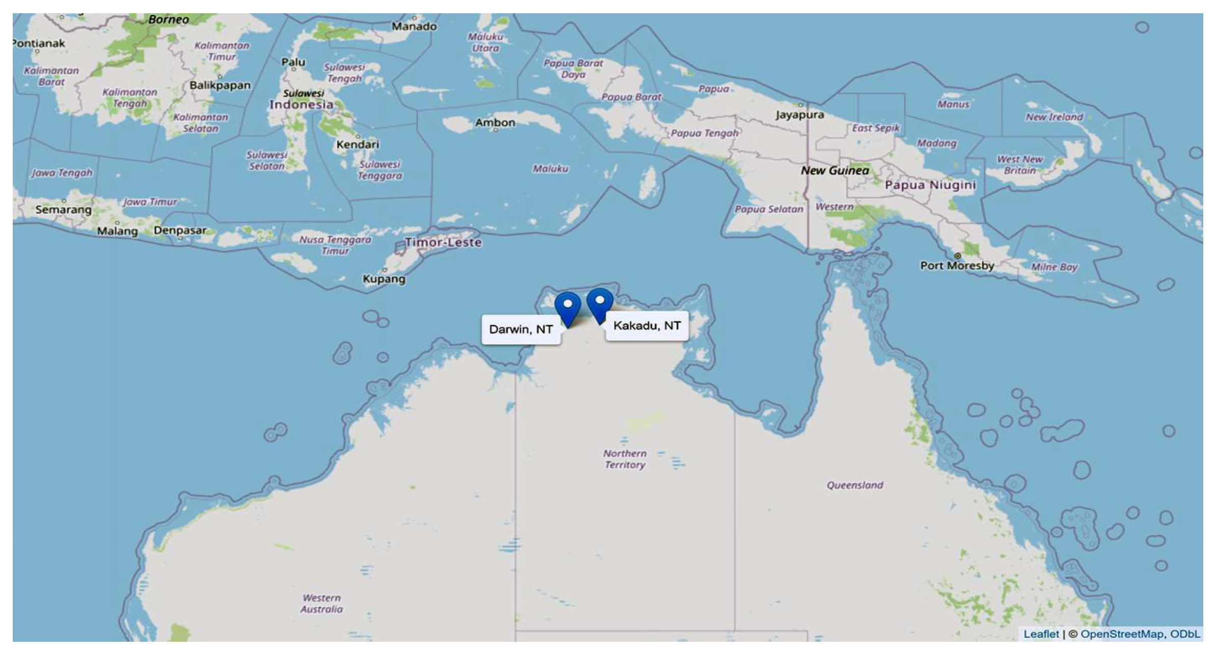
Single-frequency commercial-grade GNSS receivers on the market utilise different combinations of GNSS signals, with the GPS ones being common with all of them. For that reason, this research utilises the GPS pseudorange observations for the derivation of experimental (true) TEC. The GPS pseudorange observations taken at the IGS reference station in Darwin, NT, Australia (Figure 5), for four scenarios of geomagnetic storms identified in Section 2.3 are used in this research. The selection of the IGS Darwin reference stations was driven by its position in the sub-equatorial region, with pronounced ionospheric disturbance effects and with its proximity to the INTERMAGNET [30] Kakadu, NT, Australia, reference station. The true TEC is estimated from dual-frequency GNSS pseudorange observations using the procedure outlined in (7) (Section 1), with the GPS-TEC Programme software, revision 3.0, developed by Dr Gopi Seemala [31]. The GPS-TEC Programme deploys estimates of the satellite bias b_s as provided by the University of Bern. The receiver bias b_r is estimated by using the re-scaling standardisation procedure applied to the raw GPS TEC estimates [31].

2.5. Geomagnetic Field Density Observations at INTERMAGNET Reference Station Kakadu, NT

The INTERMAGNET operates the world network of stationary reference sites that systematically collect the observations of the geomagnetic field density vector components B_x, B_y and B_z [30]. The observation procedure requires the measurements to be taken on a daily basis, every minute. Collected observations are stored in structured text files openly available to interested parties. Observations taken at the INTERMAGNET reference station Kakadu, NT, Australia (Figure 5), for four scenarios of geomagnetic storms identified in Section 2.3 are used in the presented research.

The selection of the INTERMAGNET Kakadu reference stations as the source of geomagnetic field density observations was driven by its proximity to the IGS Darwin reference stations. The research assumes similar geomagnetic and ionospheric conditions, resulting in similar GNSS pseudorange measurement degradations, in the locations of two reference stations separated by a distance of 178.5 km.

2.6. Material Summary Per Geomagnetic Storm Scenario

As described in Section 2.2, this research utilises four sets of data (time series) per scenario: TEC values and three components of the geomagnetic field density vector. Data sets of geomagnetic field density components and the associated experimental TEC are statistically analysed to assist the development of the ambient-aware GNSS TEC prediction model for PNT in the case of short-term rapidly developing ionospheric storms. The results of the statistical analysis are presented in a box-plot form. The exploratory statistical analysis results are summarised in the rest of this section for the four scenarios defined in Section 2.3.

2.6.1. The Mid-March 2015 Geomagnetic Storm Scenario (The St Patrick’s Day 2015 Storm, Storm 1)

Box plots of predictors B_x, B_y and B_z and the experimentally derived TEC target are presented in Figure 6.

The results of the exploratory statistical analysis of related time series of TEC, B_x, B_y and B_z variables show that none of them follow a normal statistical distribution. The TEC, B_y and B_z variables extend a number of outliers, with the respective long right tails of the corresponding experimental statistical distributions. The B_x variable extends several outliers at the left tail of its experimental statistical distribution.

2.6.2. The Late-May 2017 Geomagnetic Storm Scenario (Storm 2)

Box plots of predictors B_x, B_y and B_z and the experimentally derived TEC target are presented in Figure 7.

The results of the exploratory statistical analysis of related time series of TEC, B_x, B_y and B_z variables show that none of them follow a normal statistical distribution. The TEC variable yields numerous outliers at the right tail, while the B_x and B_y variables extend outliers at the left tails of their corresponding experimental statistical distributions. Additionally, the B_y variable yields a few outliers at the right tail.

2.6.3. The Early-September 2017 Geomagnetic Storm Scenario (Storm 3)

Box plots of predictors B_x, B_y and B_z and the experimentally derived TEC target are presented in Figure 8.

The results of the exploratory statistical analysis of related time series of TEC, B_x, B_y and B_z variables show that none of them follow a normal statistical distribution. While TEC values extend a few outliers on the right tail of the statistical distribution, the B_x and B_y variables yield numerous outliers at both tails of their corresponding experimental statistical distributions.

2.6.4. The Late-September 2017 Geomagnetic Storm Scenario (Storm 4)

Box plots of predictors B_x, B_y and B_z and the experimentally derived TEC target are presented in Figure 9.

The results of the exploratory statistical analysis of related time series of variables show TEC and B_z as following a normal statistical distribution. The B_x and B_y variables experienced a number of outliers, with slight tails, left and right.

2.6.5. Analysis and Discussion

Overall, the exploratory analysis of TEC and geomagnetic field density component observations leads to the conclusion of short-term rapidly developing storms as a well-described class of space weather events affecting the GNSS positioning performance. Additional analysis is conducted to obtain a deeper insight into the nature of TEC dynamics during four geomagnetic storms under consideration. The Cullen–Frey method [32] is applied to estimate the theoretical statistical distribution that fits data in all four TEC sets concerned. The Cullen–Frey method examines the relationship between kurtosis and the square of skewness of bootstrapped samples (subsets) of the original data.

The Cullen and Frey graph analysis reveals the beta statistical distribution as the most promising fit to the experimental data of all four cases considered. Three of them extend a high similarity of the theoretical statistical distribution fit, while the May 2017 storm extends a somewhat larger square of skewness. The findings confirm the case of short-term rapidly developing geomagnetic storms as a well-defined class of GNSS-related space weather events.

Additional exploratory statistical analysis is performed to identify the processes behind TEC dynamics for all four cases of rapidly developing short-term geomagnetic storms, including the following statistical tests [33]: (i) the two-sample t-test to determine whether the means of two sets of TEC observations of different geomagnetic storms are equal, (ii) the two-sample F-test to determine whether the variances of two sets of TEC observations of different geomagnetic storms are equal and (iii) the two-sample Kolmogorov–Smirnoff test to determine whether two sets of TEC observations of different geomagnetic storms follow the same statistical distribution. The exploratory statistical analysis finds that no pairs of TEC sets share either the same mean, variance or result from the same statistical distribution. Given the complexity of the TEC generation processes, the results of the exploratory analysis confirm the expectations. Additionally, the results of statistical tests indicate the need for an advanced method for TEC correction model development. The inference leads to the selection of machine learning-based methods as a suitable approach in the solution of TEC prediction model development.

The resulting Cullen and Frey diagrams are depicted in Figure 10.

The Cullen and Fray analysis, the exploratory data analysis and statistical tests [33] are performed in the R environment for statistical computing [21] using the R package fitdistrplus [32] for the former and the standard packages for the latter analyses.

3. Research Results

We aggregate the time series of all four scenarios into a single pool of observations while keeping the variable-related structure, thus composing a set of observations as a representative sample comprising descriptions of different variances of short-term rapidly developing geomagnetic storms. The aggregated original pool consists of 13,817 observations of TEC (outcome) and B_x, B_y and B_z (predictors) variables from the four selected scenarios (Section 2.3). We split the pool of observations into training (model development) and testing (model evaluation) subsets of the original pool of observations using the 80–20 Pareto principle [34,35]. The cross-validation procedure is involved in the development of both the SGB-based and BC-based TEC prediction model candidates to mitigate the effects of a non-normal experimental distribution and randomisation involved in observation selection for training and testing subsets of the original data. The testing subset is used for the assessment of Klobuchar model performance to provide a benchmark (reference) model for additional comparisons of the quality of developed TEC prediction model candidates. 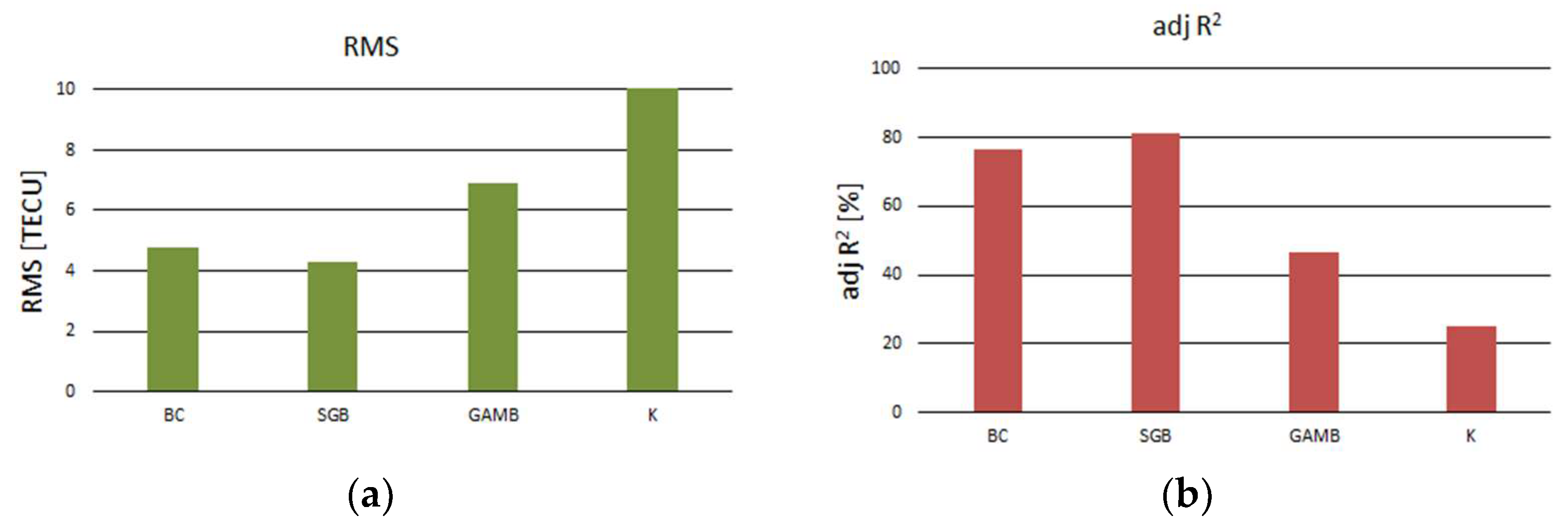Section 2.2.4 outlines the method performance assessment criteria, including root-mean-square error (RMSE) for bias modelling performance assessment, the adjusted coefficient of determination (adjR²) for variance modelling performance assessment and the P-O diagram for graphical assessment of the model agility. Model development and model performance validation tasks are performed using the tailored software our team developed in the R environment for statistical computing. Assessment results of the ability of candidate PPR-based, SGB-based, BCART-based and Klobuchar models to describe bias and variance in the testing subset are depicted in Figure 11 and outlined in

Table 1. TEC prediction model development time.

	Bagged CART (BCART)	Stochastic Gradient Boosting (SGB)	Boosted Generalized Additive Model (GAMB)
Model development time [s]	17.89	32.15	13.43

.

The Klobuchar model, the standard GPS error correction model considered a reference model in this research, performs poorly during short-term rapidly developing geomagnetic storms in sub-equatorial regions. It extends a large RMSE and describes only 25% of the original variance. Contenders for the TEC prediction model perform far better than Klobuchar, in support of the hypothesis of improved GNSS ionospheric correction estimation based solely on the near-real-time local geomagnetic field density vector observations. The PPR model reduces by nearly 30% the Klobuchar model RMSE, and doubles the original variance coverage, compared with the Klobuchar model. The BCART model halves the Klobuchar model RMSE and covers more than 76% of the original variance. The SGB-based TEC prediction model extends an even better RMSE value than the BCART model and is capable of modelling more than 81% of the original variance.

Statistical learning models develop as a result of experience. They may be designed to improve their predictive capacity and performance. The time required to complete model development may indicate the computational effort needed to develop the model as related information for GPS positioning process developers and operators. Model development times for the TEC predictive model contenders are examined, with the results presented in Table 1.

The SGB-based model requires the most time to develop, almost twice as much as needed for BCART model development. Considering the performance accomplished, the selection of the BCART model may be a good trade-off for applications where computing resources are critical. The PPR model requires just about one-fifth of the SGB model development time, which trades with a significantly reduced performance in comparison with the SGB model.

The P-O diagrams reveal the agility of the TEC model candidates, as shown in Figure 12.

Considering the performance assessment indices defined in Section 2.2.4, the stochastic gradient boosting (SGB) TEC prediction model extends the best performance during short-term rapidly developing geomagnetic storms in the sub-equatorial region of all three models assessed.

4. Discussion

This research addresses the development of the ambient-aware GNSS TEC prediction model suitable for integration within the ambient-aware GNSS PNT framework as an alternative to standard GNSS ionospheric correction models, such as the Klobuchar model. The proposed ambient-aware GNSS TEC prediction model development methodology is demonstrated in the scenario of short-term rapidly developing ionospheric storms, one of the extreme cases of ionospheric conditions that may cause significant degradation of the GNSS PNT performance. The proposed ambient-aware GNSS TEC prediction model returns the TEC estimate for the particular case of the ionospheric conditions, determined by the values of predictors (B_x, B_y and B_z) at the time of prediction.

Based on the statistical properties of four selected cases of short-term rapidly developing ionospheric storms, three ambient-aware GNSS TEC prediction models are developed and their performance is assessed and compared mutually and in relation to the Klobuchar model’s performance in the same cases. As a result, the stochastic gradient boosting (SGB) TEC prediction model is found to be the best performer in the group. The SGB GNS TEC prediction model covers bias with a root-mean-square error (RMSE) of 4.28 TECU, a 60% improvement compared with the Klobuchar model. Further to this, the stochastic gradient boosting (SGB) TEC prediction model describes 82% of the original variance in derived experimental TEC observations, compared with just 25% as extended by the Klobuchar model. The stochastic gradient boosting (SGB) TEC prediction model requires more time and effort to be developed. However, once developed, it provides the best performance, with reasonable execution time concerning deployment in modern computationally improved devices, such as smartphones, IoT devices, cars, drones and others.

The proposed GNSS TEC prediction model aims at deployment within the ambient-aware GNSS PNT framework, either on mobile devices or within the positioning-as-a-service framework. Particular concern is given to implementation on devices utilising single-frequency GNSS PNT, with the aim to provide an alternative to standardised global ionospheric correction models.

The implementation of the proposed method and the model are rather simple and straightforward in modern software-defined radio (SDR)-based GNSS receivers and even more elegant and efficient in the positioning-as-a-service distributed GNSS processes. Utilisation of the SDR concept renders the GNSS PNT process and algorithm transparent and flexible in terms of improvement of the existing PNT algorithm and for the introduction of new services by exploitation of methods and techniques of statistics, computer science and mobile communications. We demonstrated the deployment of the proposed ambient-aware GNSS TEC prediction model within a laboratory ambient-aware PNT framework, which includes the open-source RTKLIB SDR, in both real-time and post-processing simulations. In the post-processing scenario, the ionospheric corrections were calculated using the proposed ambient-aware GNSS TEC prediction model, with data structured in the IONEX format.

Sources of data may be either the mobile unit’s own measurements of the positioning environment conditions (components of the geomagnetic field in the vicinity of a GPS/GNSS receiver) using the unit’s own sensors, trusted third-party data (NOAA, NASA, EU Copernicus, INTERMAGNET, etc.) delivered through a dedicated and encrypted communications protocol via the mobile internet or both. The actual benefit achieved depends on the mobile unit’s ability to measure the geomagnetic field components accurately and correctly and on the third party’s ability to provide near-real-time data of high accuracy. Furthermore, thorough and systematic consideration should be given to communications safety and to means of deployment and operation of machine learning methods to safeguard them from adversarial cyber-attacks [36,37]. A case of geomagnetic data-based spoofing may be overcome with authentication, sensor information fusion and additional analysis of time series of data.

This research provides the proposal for the method, and its proof-of-principle justification, thus establishing a solid framework for further refinements and developments planned to be accomplished by this group. Future research will focus on model development and validation for different levels of ionospheric disturbances and ambients of PNT (geographic latitudes, urban/rural environments, inclusion of information from other ambient sensors, etc.).

5. Conclusions

Satellite navigation has become one of the pillars of modern civilisation and an essential component of the national infrastructure. Space weather and ionospheric conditions render the prime source of single-frequency GNSS PNT service disruptions and degradations. The PTA of GNSS PNT services requires novel approaches in tackling the ionospheric effects on GNSS PNT. Standard global ionospheric correction models cannot mitigate the local ionospheric disturbances, as well as those of high dynamics. A self-adaptive positioning environment-aware GNSS position estimation algorithm, which engages a bespoke machine learning-based GNSS ionospheric correction model, offers huge promises in the PTA of GNSS. Here, we show that even in the case of demanding ionospheric conditions, such as during a short-term fast-developing geomagnetic storm in a sub-equatorial region, a machine learning-based environment-aware GNSS ionospheric correction model developed and operated by a position estimation entity, either a traditional GNSS receiver or a positioning-as-a-service system, may provide a substantial improvement over the existing global Klobuchar model, which is considered as a benchmark.

This research evaluates three candidates for the ambient-aware GNSS PNT ionospheric correction models based on machine learning methods and large sets of experimental observations of geomagnetic field density components as predictors and TEC/single-frequency GPS ionospheric delay as the target. Machine learning development methods for three models are selected based on the results of the exploratory statistical analysis of predictors and target observations. The performance of the three GPS ionospheric model candidates, (i) the bagged CART model, (ii) the boosted generalized additive model (GAMB) and (iii) the stochastic gradient boosting (SGB) model, are assessed and compared with the Klobuchar model as the benchmark.

The ambient-aware SGB TEC/GNSS pseudorange measurement error predictive model is proposed as the result of the comparison, based on experimental observations and a statistical/machine learning model development technique, with the component of the geomagnetic field density vector as the sole predictor and TEC as the target. The TEC prediction model is developed and validated for GNSS ionospheric delay corrections during short-term rapidly developing geomagnetic storms in a sub-equatorial region, which significantly reduces (60%) bias error compared with standard Klobuchar model and describes 82% of the original TEC variance. The research finds D_st to be a good classifier for the ionospheric condition scenarios.

Further research is needed to refine the methodology for machine learning-based model development method selection and validation to be deployed for various classes and scenarios of ionospheric conditions and geographic latitudes, enhance the robustness of the machine learning-based model to safe-guard it against malicious attacks and establish an architecture-agnostic framework for operational deployment of the resulting optimal machine learning-based and positioning environment-aware bespoke ionospheric correction model that contributes to GNSS resilience development through advanced PTA deployment.