Distributed Phased Multiple-Input Multiple-Output Radars for Early Warning: Observation Area Generation

Abstract

This paper introduces a resource management approach for distributed multiple-input multiple-output (MIMO) radar systems equipped with phased array antennas. The approach focuses and adjusts narrow beams from all transmit and receive nodes to generate a regularly shaped observation area for reliable detection. Based on this, a structured early warning framework can be built by evenly arranging sufficient observation areas to cover the surveillance region and periodically scanning these areas for continuous monitoring. Observation area generation, a core technique for this framework, involves the joint optimization of beamforming weights for both transmit and receive nodes, as well as the beam dwell time. Our optimization strategy is designed to achieve two key objectives: minimizing beam dwell time to ensure rapid alerts for defense systems, and minimizing node transmit power to extend operational time while reducing the risk of intercept. To address the problem of observation area generation, we propose a two-stage method. The first stage uses the signal-to-clutter-plus-noise ratio (SCNR) as a new criterion to determine the transmit and receive beamforming weights. The second stage employs a power factor as an additional variable to scale the transmit beamforming weights under various beam dwell times, constructing a Pareto solution set for the problem. Numerical simulations validate the effectiveness of our method, demonstrating improved detection capabilities compared to monostatic phased array radar systems.

1. Introduction

Distributed multiple-input multiple-output (MIMO) radar systems synthesize the strengths of MIMO technology with separated architectures, thus providing significant enhancements in target detection and resolution capabilities [1,2,3,4,5]. Generally, their operating modes are categorized into two types: ubiquitous and non-ubiquitous [6]. The ubiquitous mode is characterized by broad beams at both transmit and receive nodes, which ensure complete illumination of a surveillance region without the need for beam direction adjustment. In this mode, radar systems can provide continuous and uninterrupted monitoring. In contrast, the non-ubiquitous mode utilizes high-gain, narrow beams to concentrate energy on specific targets or small areas. This mode enables radar systems to detect targets at a greater distance more quickly by sacrificing coverage in a single observation. However, selective coverage may result in unmonitored gaps within the surveillance area, which could lead to delayed threat detection. To mitigate this risk, radar systems must actively steer and focus all beams, conducting periodic scans over the entire surveillance region. Thus, effective beam scheduling is essential to achieve the early warning function in the non-ubiquitous mode [7].

1.1. Related Works and Motivation

Current research on distributed MIMO radar systems predominantly concentrates on beam scheduling for target tracking scenarios [8,9,10,11]. In these scenarios, the trajectory and motion model of a target can be used to predict its location, which is vital for effective beam scheduling. The predictability of target locations enables beam scheduling to be achieved through node assignment, i.e., a node steers its beam toward the predicted location of the target. However, early warning scenarios present more complex challenges for beam scheduling due to the unpredictability of target locations and the absence of well-defined observation areas. In distributed MIMO radars, observation areas are formed within the overlapping volume of all transmit and receive beams. Determining the coverage of observation areas based on detection performance or half-power beam width often results in irregular shapes that change with location [12]. The variability complicates the task of arranging observation areas to fully cover a surveillance region. In contrast, monostatic radars offer a more straightforward approach using beam-shaped observation areas. The half-power beam width determines the azimuth and elevation ranges of the observation areas, while the detection performance determines their distance range [13]. This feature allows for the pre-arrangement of multiple observation areas at equal angular intervals to ensure a complete coverage of the surveillance region. This approach, referred to as beam arrangement [14,15], raises a question of whether distributed MIMO radar systems can generate regularly shaped observation areas suitable for uniform arrangement. Fortunately, the advanced beamforming capability of phased array antennas, which offers the flexibility and precision required for effective beam steering and shaping, is the necessary technical foundation to achieve this.

Phased array antennas are capable of changing the shape and direction of beams without physical movements, which makes them widely applied in fields such as aviation, defense and wireless communication [16,17,18]. Distributed MIMO radars with phased array antennas, also called distributed phased MIMO radars, can independently control the shape and direction of the beam at each node. These systems have the ability to mold observation areas into regular shapes for uniform arrangement through the adjustment of focused transmit and receive beams. Once these areas are prearranged, they become the fundamental units for resource allocation, allowing radar systems to focus on core functions such as early warning and target tracking, rather than detailed beam resource management. This process also introduces a new challenge: the beamforming problem. In recent years, many references have studied this problem [19,20,21,22,23,24,25]. Most of them focus on collocated MIMO radars, making great contributions to improving radar performance in terms of signal-to-interference-plus-noise ratio [19,20,21,22], power consumption [19], and beam pattern peak side-lobe level [19,25]. Collocated MIMO radars typically require the estimation of the direction of arrival, the angles of arrival, and the time delays [26,27,28]. The elements of collocated MIMO radars satisfy the far-field assumption, which ensures that the direction from each element to a target is the same. As a result, beamforming is tasked to concentrate the beam energy in the azimuth and elevation directions of the target. However, these methods are not directly applicable to distributed MIMO radars. For distributed MIMO radars with widely separated nodes, the far-field assumption does not hold between elements of different nodes. Moreover, these systems must control the accumulation of beam energy in a three-dimensional space. Therefore, there is a need for a beamforming method that integrates the capabilities of all nodes.

1.2. Contributions

On the basis of the above reasons, in this paper, we examine an approach for generating a predefined observation area in a typical non-ubiquitous mode, i.e., the focused-transmit focused-receive (FTFR) operating mode. This approach allows distributed phased MIMO radars to adjust the spatial distribution of detection performance by optimizing the transmit and receive beamforming weights and the beam dwell time. Our main contributions are summarized as follows:

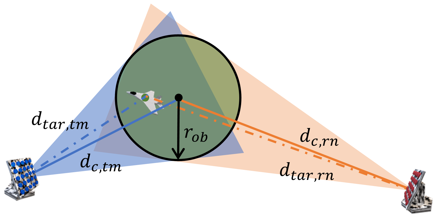
• A mathematical model for evaluating the detection performance of distributed MIMO radars with widely separated phased array antennas is developed. This model considers the correlation of target echoes received in different channels by extending the target model in [29] from circle to sphere. Meanwhile, it also considers a ground clutter environment based on the bistatic radar clutter model in [30].
• An optimization strategy for the generation of observation areas is presented. There is an inherent trade-off under fixed detection coverage and performance requirements: a shorter beam dwell time demands increased transmit power. Although a shorter dwell time accelerates target detection, increased transmit power raises the risk of intercept. To balance radar detection efficiency and survivability, our optimization strategy minimizes the transmit power and beam dwell time of the nodes. In addition, we consider the worst case for targets to be detected, similar to [7].
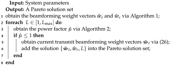
• A two-stage method for solving the problem of observation area generation is proposed. To separately optimize the beamforming weights and the beam dwell time, we introduce the signal-to-clutter-plus-noise ratio (SCNR) as a criterion and a power factor as a variable. The first stage jointly optimizes the transmit and receive beamforming weights to balance the SCNRs of all transmit–receive channels at all cells under test (CUT) within an observation area. Linearized successive convex approximation (SCA) and trust region techniques [31] are used to solve this optimization problem. The second stage optimizes the power factor under various beam dwell times to scale down the transmit beamforming weights. A binary search method is used to build a Pareto solution set for the original problem.

This paper is structured as follows. Section 2 presents the system model, Section 3 formulates the observation area generation problem and proposes a solving method. Section 4 and Section 5 provide the simulations, analysis, and discussion. Finally, Section 6 concludes this paper. The basic notations and symbols are shown in

Table 1. The table of notations and symbols.

Notation	Meaning
${(·)}^{*}$	conjugate operation
${(·)}^H$	conjugate transpose operation
${(·)}^{†}$	transpose operation
$max\{·\}$	extract the maximum element
$min\{·\}$	extract the minimum element
$\lfloor ·\rfloor$	round down to the closest integer
${cos}^{-1}(·)$	arc cosine function
${tan}^{-1}(·)$	arc tangent function
⊗	Kronecker product
⊙	element-wise multiplication
$\mathbb{E}$	statistical expectation
$\mathrm{blkdiag}\{·\}$	block diagonal matrix created by the elements
Symbol	Meaning
${\mathbb{Z}}^{+}$	a set of positive integers
$\mathbb{C}$	a set of complex numbers
${[X_{·},Y_{·},Z_{·}]}^{†}$	global rectangular coordinates
${[x_{·},y_{·},z_{·}]}^{†}$	local rectangular coordinates
$({\vartheta }_{·},{\phi }_{·},d_{·})$	spherical coordinates (in a node coordinate system)
$({\theta }_{·},{\varphi }_{·},r_{·})$	spherical coordinates (in a target coordinate system)
${\Theta }_{·}$	global azimuth angle
${\Phi }_{·}$	global elevation angle
${\mathbf{I}}_{·}$	unit matrix/identity matrix

.

2. System Model and Detection Performance

  Consider a distributed MIMO radar system with M transmit nodes and N receive nodes, as shown in Figure 1. Each node is equipped with a phased array antenna and is widely separated from the others. We have made several foundational assumptions to clearly describe the system model:

• Each node is equipped with a uniform planar array antenna and has an identical number of elements.
• For each node, the far-field assumption is valid, i.e., all elements of a node share the same beam propagation direction towards any target or CUT.
• The radar system is assumed to be perfectly calibrated, for example, using GPS satellites [32], allowing for the ignoring of time synchronization errors between different nodes.

Figure 1. Geometry of a distributed MIMO radar system.

Figure 1. Geometry of a distributed MIMO radar system.

The geometric configuration of the radar system is established within a ground coordinate system, O-$XYZ$, which serves as a global reference frame. The $XY$ plane coincides with the ground plane and the Z axis is perpendicular to it. In the ground coordinate system, the planar centers of the mth transmit node and the nth receive node are located at ${\mathbf{X}}_{tm}={[X_{tm},Y_{tm},Z_{tm}]}^{†}$ and ${\mathbf{X}}_{rn}={[X_{rn},Y_{rn},Z_{rn}]}^{†}$, respectively, where $m=1,\dots ,M$ and $n=1,\dots ,N$. There is a surveillance region that has been divided into multiple cubic cells under test (CUTs). Assume that an observation area contains K CUTs. The center of the kth CUT is located at ${\mathbf{X}}_{vk}={[X_{vk},Y_{vk},Z_{vk}]}^{†}$, where $k=1,\dots ,K$. To define steering vectors and radiation patterns, a node coordinate system is established for each node. This coordinate system serves as a local reference frame. The origin is located in the planar center of the node. The x axis is along the boresight direction, i.e., the normal direction of the planar antenna, and the $xz$ plane remains perpendicular to the ground plane. The global rectangular coordinates of the kth CUT can be converted to the local spherical coordinates by

$$\left\{\begin{array}{cc}\hfill {\vartheta }_{k,★}& ={cos}^{-1}(x_{k,★}/\sqrt{x_{k,★}^2+y_{k,★}^2}),\hfill \\ \hfill {\phi }_{k,★}& ={tan}^{-1}(z_{k,★}/\sqrt{x_{k,★}^2+y_{k,★}^2}),\hfill \\ \hfill d_{k,★}& =\sqrt{x_{k,★}^2+y_{k,★}^2+z_{k,★}^2},\hfill \end{array}\right.$$

(1)

with

$${\mathbf{x}}_{k,★}={\left[\begin{array}{c}{x}_{k,★},y_{k,★},z_{k,★}\end{array}\right]}^{†}={\mathbf{R}}_{★}^{†}·({\mathbf{X}}_{vk}-{\mathbf{X}}_{★}),$$

where $★=tm,rn$. ${\mathbf{X}}_{★}$ is the planar center of each node. ${\vartheta }_{k,★}$ and ${\phi }_{k,★}$ are the azimuth and elevation angles of the beam propagation direction, respectively. $d_{k,★}$ is the distance between the node and the kth CUT. ${\mathbf{x}}_{k,★}$ is the local rectangular coordinates. ${\mathbf{R}}_{★}$, the rotation matrix for the transformation from the local coordinates to the global coordinates, is given by [33]

$${\mathbf{R}}_{★}=\left[\begin{array}{ccc}cos{\Theta }_{★}& -sin{\Theta }_{★}& 0\\ sin{\Theta }_{★}& cos{\Theta }_{★}& 0\\ 0& 0& 1\end{array}\right]\left[\begin{array}{ccc}cos{\Phi }_{★}& 0& -sin{\Phi }_{★}\\ 0& 1& 0\\ sin{\Phi }_{★}& 0& cos{\Phi }_{★}\end{array}\right].$$

Based on the local spherical coordinates in (1), the steering vector of the kth CUT in the $(m,n)$ channel is given by [34]

$${\tilde{\mathit{\alpha }}}_{k,★}={\tilde{\mathit{\alpha }}}_y({\vartheta }_{k,★},{\phi }_{k,★})\otimes {\tilde{\mathit{\alpha }}}_z\left({\phi }_{k,★}\right)\in {\mathbb{C}}^{U\times 1},$$

(2)

with

$$\begin{array}{cc}\hfill {\tilde{\mathit{\alpha }}}_y({\vartheta }_{k,★},{\phi }_{k,★})& ={\left[\begin{array}{c}\dots ,exp\left\{j{\displaystyle \frac{2\pi f_c}{c}}{y}_{★,u}sin{\vartheta }_{k,★}cos{\phi }_{k,★,}\right\},\dots \end{array}\right]}^{†}\in {\mathbb{C}}^{U_{col}\times 1},\hfill \\ \hfill {\tilde{\mathit{\alpha }}}_z\left({\phi }_{k,★}\right)& ={\left[\begin{array}{c}\dots ,exp\{j{\displaystyle \frac{2\pi f_c}{c}}{z}_{★,u^{\prime }}sin{\phi }_{k,★}\},\dots \end{array}\right]}^{†}\in {\mathbb{C}}^{U_{row}\times 1},\hfill \\ \hfill y_{★,u}& =\Delta d_{e,col}·(u-(U_{col}+1)/2),u=1,\dots ,U_{col},\hfill \\ \hfill z_{★,u^{\prime }}& =\Delta d_{e,row}·(u^{\prime }-(U_{row}+1)/2),u^{\prime }=1,\dots ,U_{row},\hfill \end{array}$$

where $f_c$ is the carrier frequency. c is the light speed. $U=U_{col}{U}_{row}$ is the total element number. $U_{col}$ and $U_{row}$ are the element numbers in the column and row directions, respectively. $(0,y_{★,u},z_{★,u^{\prime }})$ are the rectangular coordinates of elements in the node coordinate system. $\Delta d_{e,col}$ and $\Delta d_{e,row}$ are the intervals between adjacent elements in column and row directions. Assume that all elements have a Gaussian radiation pattern [35]. The radiation pattern of elements is

$$G_{k,★}=G_{0}exp\left\{-2.773\left({\vartheta }_{k,★}^2/{\vartheta }_{3dB,★}^2+{\phi }_{k,★}^2/{\phi }_{3dB,★}^2\right)\right\},$$

(3)

where $G_0=4\pi /({\vartheta }_{3dB,★}·{\phi }_{3dB,★})$ is the peak element gain. ${\vartheta }_{3dB,★}$ and ${\phi }_{3dB,★}$ are the 3 dB beam widths of elements in the azimuth and elevation directions.

In the following subsections, a mathematical model will be developed to evaluate the detection capability of the distributed MIMO radar at the kth CUT.

2.1. Target Echo Model

Consider a moving target located at the kth CUT, which consists of Q scattering points. This target remains within the kth CUT before each channel has received at least L consecutive pulses. In early warning scenarios, target attitude is typically unknown. For analytical purposes, we consider a spherical target with isotropic scattering characteristics. Let $(\theta ,\varphi ,r)$ denote the local spherical coordinates of a point in the target coordinate system, as shown in Figure 2. The origin is located at the sphere center, i.e., the target center. The axes of the target coordinate system are parallel to those of the ground coordinate system. The normalized scattering coefficient at this point is given by [29]

$$\tilde{\eta }(\theta ,\varphi ,r)=\sum _{q=1}^Q{\tilde{\nu }}_q·\delta (\theta -{\theta }_q)·\delta (\varphi -{\varphi }_q)·\delta (r-r_q),$$

where $\delta (·)$ is a Dirac delta function. $({\theta }_q,{\varphi }_q,r_q)$ is the local spherical coordinates of the qth scattering point. ${\tilde{\nu }}_q\sim \mathcal{CN}(0,1/V)$ is the scattering intensity that follows a Gaussian distribution of zero mean. $V=\left(4\pi r_{size}^3\right)/3$ is the target volume and $r_{size}$ is the sphere radius, i.e., the target size. By integrating all echoes from points within the target, the target echo received at the nth node can be expressed as

$${\tilde{y}}_{k,n}\left(t\right)=\sum _{m=1}^M\sum _{\ell =1}^L{\int \int \int }_{\Omega }{\tilde{a}}_{k,m,n}{h}_{k,m,n}{\tilde{e}}_{k,m,n,\ell }(\theta ,\varphi ,r)·\tilde{\eta }(\theta ,\varphi ,r)·{\tilde{s}}_m(t-{\tau }_{k,m,n,\ell })\mathrm{d}\Omega ,$$

(4)

where $\Omega$ is the space covered by the target. ${\tilde{a}}_{k,m,n}$ is the $(m,n)$ channel response. $h_{k,m,n}$ is path loss. ${\tau }_{k,m,n,\ell }$ is the time delay. ${\tilde{s}}_m$ is the baseband signal transmitted by the mth transmit node. ${\tilde{e}}_{k,m,n,\ell }$, which is the phase term caused by target motion, is [13]

$${\tilde{e}}_{k,m,n,\ell }=exp\left\{-j{\displaystyle \frac{2\pi }{\lambda }}\left(d_{m,n,0}(\theta ,\varphi ,r)-v_{m,n}·\left(\ell T_{PRI}+{\displaystyle \frac{d_{m,n,\ell }(\theta ,\varphi ,r)}{c}}\right)\right)\right\},$$

(5)

where $d_{m,n,0}$ and $d_{m,n,\ell }$ are the bistatic path length at the initial time and the ℓth sample time. $v_{m,n}$ is the projection of the target velocity in the $(m,n)$ channel. Note that the distance between the target and any node is much greater than both the edge length of the CUTs and the target size. Thus, the variations in channel response and path loss can be neglected for different points within the target. Using the steering vector for the kth CUT in (2), the $(m,n)$ channel response with known transmit and receive beamforming weight vectors ${\tilde{\mathit{w}}}_{tm}$ and ${\tilde{\mathit{w}}}_{rn}\in {\mathbb{C}}^{U\times 1}$ is

$${\tilde{a}}_{k,m,n}={\tilde{\mathit{w}}}_{rn}^H{\tilde{\mathit{\alpha }}}_{k,rn}{\tilde{\mathit{\alpha }}}_{k,tm}^H{\tilde{\mathit{w}}}_{tm}.$$

(6)

Based on the radiation pattern in (3), the corresponding path loss is [36]

$$h_{k,m,n}=\sqrt{{\displaystyle \frac{{\lambda }^2{\sigma }_{m,n}^2{G}_{k,tm}{G}_{k,rn}}{{\left(4\pi \right)}_3{d}_{k,tm}^2{d}_{k,rn}^2{\mathcal{L}}_{k,m,n}}}},$$

(7)

where $\lambda$ is the wave length. ${\sigma }_{m,n}^2$ is the radar cross-section (RCS) of the target in the channel. ${\mathcal{L}}_{k,m,n}$ is the system loss.

2.2. Ground Clutter Echo Model

Consider the $(m,n)$ channel shown in Figure 3. A channel coordinate system is built with the midpoint of the baseline projection as the origin $O_{m,n}$. The x axis is along the baseline projection on the ground plane and the z axis is perpendicular to the ground plane. Note that the distance from the nodes to the clutter belt is much greater than the height of these nodes. The clutter belt can be approximated by the area between two ellipses with the projection coordinates of the two nodes as the focal points. We then partition the clutter belt into B non-overlapping surfaces with an angular interval of $\Delta \theta$. Specifically, $\Delta \theta$ is defined as $2\pi /B$. The centers of these clutter surfaces are distributed approximately along an elliptical path. For the kth CUT, the semi-major axis and the semi-minor axis of the ellipse are

$$\begin{array}{cc}\hfill & {\mathcal{a}}_{k,m,n}={\displaystyle \frac{1}{2}}(d_{k,tm}+d_{k,rn}),\hfill \\ \hfill & {\mathcal{b}}_{k,m,n}={\displaystyle \frac{1}{2}}\left\{\sqrt{{({\mathcal{a}}_{k,m,n}-\Delta ϵ/2)}^2-{\mathcal{c}}_{m,n}^2}+\sqrt{{({\mathcal{a}}_{k,m,n}+\Delta ϵ/2)}^2-{\mathcal{c}}_{m,n}^2}\right\},\hfill \end{array}$$

with

$${\mathcal{c}}_{m,n}={\displaystyle \frac{1}{2}}\sqrt{{(X_{tm}-X_{rn})}^2+{(Y_{tm}-Y_{rn})}^2},$$

where $\Delta ϵ$ is the edge length of CUTs. The center coordinates of the bth clutter surface are described by a parametric representation of an ellipse:

$${\mathit{x}}_{k,b,m,n}=\left[\begin{array}{c}{x}_{k,b,m,n}\\ y_{k,b,m,n}\\ z_{k,b,m,n}\end{array}\right]=\left[\begin{array}{c}{\mathcal{a}}_{k,m,n}cos(\Delta \theta ·\left(b-1\right))\\ {\mathcal{b}}_{k,m,n}sin(\Delta \theta ·\left(b-1\right))\\ 0\end{array}\right],$$

where $b=1,\dots ,B$. Assume that each clutter surface is composed of multiple scattering points. By integrating all echoes from points within these clutter surfaces, the clutter echo received at the nth node is

$${\tilde{c}}_{k,n}\left(t\right)=\sum _{m=1}^M\sum _{\ell =1}^L\sum _{b=1}^B{\int \int }_{\mathit{x}\in {\Omega }_{k,b,m,n}}{\tilde{a}}_{k,b,m,n}{h}_{k,b,m,n}{\tilde{e}}_c\left(\mathit{x}\right)·{\tilde{\eta }}_c\left(\mathit{x}\right)·{\tilde{s}}_m(t-{\tau }_{k,m,n,\ell })\mathrm{d}\mathit{x},$$

where ${\Omega }_{k,b,m,n}$ is the space occupied by the bth clutter surface in the $(m,n)$ channel. ${\tilde{a}}_{k,b,m,n}$ is the channel response of the clutter surface. $h_{k,b,m,n}$ is the path loss. ${\tilde{e}}_c$ is the phase term caused by internal motion in clutter surfaces. ${\tilde{\eta }}_c$ is the normalized scattering coefficient of clutter. Note that the distance from the centers of the clutter surfaces to any node is much greater than the size of a clutter surface. Thus, the differences in channel response and path loss for different points within a clutter surface are ignored. Let $({\vartheta }_{k,b,★},{\phi }_{k,b,★},d_{k,b,★})$ denote the spherical coordinates of ${\mathbf{x}}_{k,b,m,n}$ in the node coordinate system. The center coordinates of the clutter surface can be transformed into the ground coordinate system by

$${\mathbf{X}}_{k,b,m,n}={\mathbf{R}}_{m,n}{\mathbf{x}}_{k,b,m,n}+{\mathbf{X}}_{m,n},$$

with

$${\mathbf{R}}_{m,n}=\left[\begin{array}{ccc}cos{\Theta }_{m,n}& -sin{\Theta }_{m,n}& 0\\ sin{\Theta }_{m,n}& cos{\Theta }_{m,n}& 0\\ 0& 0& 1\end{array}\right],$$

where ${\mathbf{R}}_{m,n}$ is the rotation matrix. ${\Theta }_{m,n}$ is the azimuth angle of the x axis of the channel coordinate system. ${\mathbf{X}}_{m,n}={[(X_{tm}+X_{rn})/2,(Y_{tm}+Y_{rn})/2,0]}^{†}$ is the translation vector between two coordinate systems. By replacing ${\mathbf{X}}_{vk}$ in (1) with ${\mathbf{X}}_{k,b,m,n}$, we can obtain the spherical coordinates of ${\mathbf{x}}_{k,b,m,n}$ in the node coordinate system. Substituting into (2) and (6), the channel response of the clutter surface can be expressed as

$${\tilde{a}}_{k,b,m,n}={\tilde{\mathit{w}}}_{rn}^H{\tilde{\mathit{\alpha }}}_{k,b,rn}{\tilde{\mathit{\alpha }}}_{k,b,tm}^H{\tilde{\mathit{w}}}_{tm},$$

where ${\tilde{\mathit{\alpha }}}_{k,b,tm}$ and ${\tilde{\mathit{\alpha }}}_{k,b,rn}$ are the steering vector of the mth transmit node and nth receive node at the bth clutter surface, respectively. Substituting into (3), we can obtain the radiation pattern of elements in these two nodes denoted by $G_{k,b,tm}$ and $G_{k,b,rn}$. $h_{k,b,m,n}$, the path loss similar to (7), is then given by

$$h_{k,b,m,n}=\sqrt{{\displaystyle \frac{{\lambda }^2{\sigma }_{k,b,m,n}^2{G}_{k,b,tm}{G}_{k,b,rn}}{{\left(4\pi \right)}_3{d}_{k,b,tm}^2{d}_{k,b,rn}^2{\mathcal{L}}_{k,b,m,n}}}},$$

where ${\sigma }_{k,b,m,n}^2={\gamma }_{k,b,m,n}\Delta s_{k,b,m,n}$ is the RCS of the clutter surface determined by the constant gamma model [35]. $\Delta s_{k,b,m,n}=\Delta ϵ\Delta \theta \parallel {\mathit{x}}_{k,b,m,n}\parallel$ is the area of the clutter surface. ${\gamma }_{k,b,m,n}={\gamma }_0\sqrt{sin{\psi }_{k,b,tm}sin{\psi }_{k,b,rn}}$ is the clutter reflectivity. ${\gamma }_0$ is a normalized reflectivity parameter. ${\psi }_{k,b,tm}$ and ${\psi }_{k,b,rn}$ are the grazing angles of the mth transmit node and the nth receive node on the clutter surface.

2.3. Radar Detection Performance

This subsection derives a detector based on the likelihood ratio test. Assume that all parameters of the above models are known. Target echoes, ground clutter echoes, and noise are statistically independent. The detector provides the best detection capability of the distributed MIMO radar.

Based on the target echo and ground clutter echo, the received signal at the nth node is

$${\tilde{r}}_{k,n}\left(t\right)={\tilde{y}}_{k,n}\left(t\right)+{\tilde{c}}_{k,n}\left(t\right)+{\tilde{n}}_n\left(t\right),$$

(8)

where ${\tilde{n}}_n\left(t\right)$ is the zero-mean white noise at the nth receive node. Assume the transmit signals from different transmit nodes are strictly orthogonal, i.e., the transmit signals satisfy the following condition:

$$\int {\tilde{s}}_m\left(t\right){\tilde{s}}_{m^{\prime }}^{*}\left(t\right)\mathrm{d}t=\left\{\begin{array}{cc}1,& m=m^{\prime },\\ 0,& m\ne m^{\prime }.\end{array}\right.$$

The matched filter outputs of all receive nodes can be expressed in vector form as

$${\tilde{\mathbf{r}}}_k={[\underset{{\tilde{\mathbf{r}}}_{k,1,1}}{\underbrace{{\tilde{r}}_{k,1,1,1},\cdots ,{\tilde{r}}_{k,1,1,L}}},\cdots ,\underset{{\tilde{\mathbf{r}}}_{k,M,N}}{\underbrace{{\tilde{r}}_{k,M,N,1},\cdots ,{\tilde{r}}_{k,M,N,L}}}]}^{†}\in {\mathbb{C}}^{MNL\times 1},$$

(9)

with

$$\begin{array}{cc}\hfill {\tilde{r}}_{k,m,n,\ell }& ={\tilde{y}}_{k,m,n,\ell }+{\tilde{c}}_{k,m,n,\ell }+{\tilde{n}}_{k,m,n,\ell },\hfill \\ \hfill {\tilde{y}}_{k,m,n,\ell }& ={\tilde{a}}_{k,m,n}{h}_{k,m,n}{\int \int \int }_{\Omega }{\tilde{e}}_{k,m,n,\ell }(\theta ,\varphi ,r)·\tilde{\eta }(\theta ,\varphi ,r)\mathrm{d}\Omega ,\hfill \\ \hfill {\tilde{c}}_{k,m,n,\ell }& =\sum _{b=1}^B{\tilde{a}}_{k,b,m,n}{h}_{k,b,m,n}{\int \int }_{\mathit{x}\in {\Omega }_{k,b,m,n}}{\tilde{e}}_c\left(\mathit{x}\right)·{\tilde{\eta }}_c\left(\mathit{x}\right)\mathrm{d}\mathit{x},\hfill \end{array}$$

where ${\tilde{n}}_{k,m,n,\ell }\sim \mathcal{CN}(0,{\tilde{\mathit{\omega }}}_{rn}^H{\tilde{\mathit{\omega }}}_{rn}{\sigma }_{\tilde{\mathit{n}}}^2)$ is the thermal noise sampled in the ℓth pulse in the $(m,n)$ channel. ${\sigma }_{\tilde{\mathit{n}}}^2=k_0{T}_0{B}_{\tilde{\mathit{n}}}$ is the noise power of the elements. $k_0$ is the Boltzmann constant. $T_0$ is the “standard” noise temperature. $B_{\tilde{\mathit{n}}}$ is the receiver noise bandwidth. If the intensities of all scattering points are independent and follows a zero-mean complex Gaussian distribution, then, due to the Central Limit Theorem when the number of scattering points is sufficiently large, the target echo is normally distributed with mean zero and variance determined by the square of the magnitude of the product of the channel response and path loss, i.e., ${\tilde{y}}_{k,m,n,\ell }\sim \mathcal{CN}(0,\parallel {\tilde{a}}_{k,m,n}{h}_{k,m,n}{\parallel }^2)$. Similarly, we have ${\tilde{c}}_{k,m,n,\ell }\sim \mathcal{CN}(0,{\sum }_b\parallel {\tilde{a}}_{k,b,m,n}{h}_{k,b,m,n}{\parallel }^2)$.

The matched filter outputs only contain ground clutter echoes and noise in the hypothesis ${\mathcal{H}}_0$. They also contain target echoes under the ${\mathcal{H}}_1$ hypothesis. Thus, the target detection problem can be formulated as a binary hypothesis test:

$${\tilde{\mathbf{r}}}_k=\left\{\begin{array}{cc}{\tilde{\mathbf{c}}}_k+{\tilde{\mathbf{n}}}_k,\hfill & \hfill {\mathcal{H}}_0,\\ {\tilde{\mathbf{y}}}_k+{\tilde{\mathbf{c}}}_k+{\tilde{\mathbf{n}}}_k,\hfill & \hfill {\mathcal{H}}_1.\end{array}\right.$$

The covariance matrix of ${\tilde{\mathbf{r}}}_k$ under these hypotheses is a square diagonal matrix:

$${\Sigma }_i=\mathbb{E}\left({\tilde{\mathbf{r}}}_k{\tilde{\mathbf{r}}}_k^H\right|{\mathcal{H}}_i)=\mathrm{blkdiag}\{{\Sigma }_{i,1},\dots ,{\Sigma }_{i,m},\dots ,{\Sigma }_{i,M}\},$$

(10)

with

$$\begin{array}{cc}\hfill {\Sigma }_{0,m}& =\mathrm{blkdiag}\left\{\mathbb{E}\left({\tilde{\mathbf{c}}}_{k,m,n}{\tilde{\mathbf{c}}}_{k,m,n}^H\right)\right|n=1,\dots ,N\}+\mathrm{blkdiag}\left\{{\tilde{\mathit{\omega }}}_{rn}^H{\tilde{\mathit{\omega }}}_{rn}{\sigma }_{\tilde{\mathbf{n}}}^2{\mathbf{I}}_{L\times L}\right|n=1,\dots ,N\},\hfill \\ \hfill {\Sigma }_{1,m}& =\mathbb{E}\left({\tilde{\mathbf{y}}}_{k,tm}{\tilde{\mathbf{y}}}_{k,tm}^H\right)+{\Sigma }_{0,m},\hfill \\ \hfill {\tilde{\mathbf{y}}}_{k,tm}& ={[{\tilde{\mathbf{y}}}_{k,m,1}^{†},\dots ,{\tilde{\mathbf{y}}}_{k,m,N}^{†}]}^{†},\hfill \end{array}$$

where $i=0,1$. Due to the orthogonality of the signals transmitted by the transmit nodes, the target echoes received from different transmit nodes are uncorrelated, i.e.,  $\mathbb{E}\left({\tilde{\mathbf{y}}}_{k,tm}{\tilde{\mathbf{y}}}_{k,t{m}^{\prime }}^H\right)=\mathbf{0}$ if $m\ne m^{\prime }$. Furthermore, since the clutter belts in different channels are spatially distinct, the echoes from different clutter belts are not correlated, i.e., $\mathbb{E}\left({\tilde{\mathbf{c}}}_{k,m,n}{\tilde{\mathbf{c}}}_{k,m^{\prime },n^{\prime }}^H\right)=\mathbf{0}$ if $m\ne m^{\prime }$ or $n\ne n^{\prime }$. Noise is assumed to be independent in both time and space. Note that our system model takes into account the spatial and temporal correlations of the target echoes, and the temporal correlations of echoes from the same clutter belt. The specific methods for calculating the covariance of the matched filter outputs are detailed in Section 4.

The joint probability density functions (PDFs) in the hypothesis satisfy the following conditions:

$$\begin{array}{c}\hfill \mathcal{P}\left({\tilde{\mathbf{r}}}_k\right|{\mathcal{H}}_0)\propto exp\{-{\tilde{\mathbf{r}}}_k^H{\Sigma }_0^{-1}{\tilde{\mathbf{r}}}_k\},\\ \hfill \mathcal{P}\left({\tilde{\mathbf{r}}}_k\right|{\mathcal{H}}_1)\propto exp\{-{\tilde{\mathbf{r}}}_k^H{\Sigma }_1^{-1}{\tilde{\mathbf{r}}}_k\},\end{array}$$

with

$$\begin{array}{cc}\hfill & {\Sigma }_0={\Sigma }_{{\tilde{\mathbf{c}}}_k}+{\Sigma }_{{\tilde{\mathbf{n}}}_k},\hfill \\ \hfill & {\Sigma }_1={\Sigma }_{{\tilde{\mathbf{y}}}_k}+{\Sigma }_{{\tilde{\mathbf{c}}}_k}+{\Sigma }_{{\tilde{\mathbf{n}}}_k},\hfill \end{array}$$

By ignoring constant items, a test statistic can be defined as

$$\begin{array}{c}\hfill T\left({\tilde{\mathbf{r}}}_k\right)={\displaystyle \frac{log\left(\mathcal{P}\left({\tilde{\mathbf{r}}}_k\right|{\mathcal{H}}_1)\right)}{log\left(\mathcal{P}\left({\tilde{\mathbf{r}}}_k\right|{\mathcal{H}}_0)\right)}}={\tilde{\mathbf{r}}}_k^H({\Sigma }_0^{-1}-{\Sigma }_1^{-1}){\tilde{\mathbf{r}}}_k.\end{array}$$

To obtain the PDF of the test statistic, we normalize ${\tilde{\mathbf{r}}}_k$. Then, the test statistic can be rewritten as

$$T\left({\tilde{\mathbf{r}}}_k\right|{\mathcal{H}}_i)={\tilde{\mathbf{r}}}_k^H{\Lambda }_i{\tilde{\mathbf{r}}}_k,$$

where ${\Lambda }_i$ is a diagonal matrix whose diagonal elements are the eigenvalues of ${\Sigma }_i^{1/2}({\Sigma }_0^{-1}-{\Sigma }_1^{-1}){\Sigma }_i^{1/2}$. ${\tilde{\mathbf{r}}}_k$ has the property that ${\tilde{\mathbf{r}}}_k\sim \mathcal{CN}(0,{\mathbf{I}}_{MNL})$. The rewritten test statistic follows a weighted chi-square distribution. Thus, the false alarm probability and detection probability are approximated by [37]

$$\begin{array}{cc}\hfill & {\mathcal{P}}_{fa}=\mathcal{P}(T\left({\tilde{\mathbf{r}}}_k\right|{\mathcal{H}}_0)\ge \gamma )=1-Q_{\Gamma }(\gamma ,{\Lambda }_0),\hfill \\ \hfill & {\mathcal{P}}_d=\mathcal{P}(T\left({\tilde{\mathbf{r}}}_k\right|{\mathcal{H}}_1)\ge \gamma )=1-Q_{\Gamma }(\gamma ,{\Lambda }_1),\hfill \end{array}$$

(11)

where $\gamma$ is the detection threshold. $Q_{\Gamma }$ is the incomplete gamma function, and its probability density function is

$$f\left(z\right)={\displaystyle \frac{{\beta }^{\alpha }{z}^{\alpha -1}}{\Gamma \left(\alpha \right)}}{e}^{-\beta z},$$

with

$$\begin{array}{cc}\hfill & \alpha =\mathrm{Tr}{\left\{{\Lambda }_i\right\}}^2/\left(4\mathrm{Tr}\left\{{\Lambda }_i^2\right\}\right),\hfill \\ \hfill & \beta =2\mathrm{Tr}\left\{{\Lambda }_i^2\right\}/\left(\mathrm{Tr}\left\{{\Lambda }_i\right\}\right).\hfill \end{array}$$

Thus, for a given false alarm probability, we can obtain the detection probability by

$${\mathcal{P}}_d=1-Q_{\Gamma }(Q_{\Gamma }^{-1}(1-{\mathcal{P}}_{fa},{\Lambda }_0),{\Lambda }_1).$$

(12)

Echo data from different channels can be matched using a grid-based method [38]. For this observation area, the multiple target detection problem can be transformed into K single-target detection problems by searching from cell to cell.

3. Optimization Problem and Solving Method

  In this section, we formulate observation area generation as a bi-objective programming problem and then propose a two-stage method to solve it.

3.1. Observation Area Generation Problem

Mathematically, observation area generation incorporates optimizing the beamforming weights and the beam dwell time under the transmit power budget and detection performance requirement. Thus, the decision variables can be divided into two types. One is the transmit and receive beamforming weights, which can be expressed in a set form as

$$\begin{array}{cc}\hfill {\tilde{\mathit{w}}}_t& =\{{\tilde{\mathit{w}}}_{t1},\dots ,{\tilde{\mathit{w}}}_{tm},\dots ,{\tilde{\mathit{w}}}_{tM}\},\hfill \\ \hfill {\tilde{\mathit{w}}}_r& =\{{\tilde{\mathit{w}}}_{r1},\dots ,{\tilde{\mathit{w}}}_{rn},\dots ,{\tilde{\mathit{w}}}_{rN}\},\hfill \end{array}$$

with

$$\begin{array}{cc}\hfill {\tilde{\mathit{w}}}_{tm}& ={\left[\begin{array}{c}{\tilde{w}}_{tm,1},\dots ,{\tilde{w}}_{tm,u},\dots ,{\tilde{w}}_{tm,U}\end{array}\right]}^{†}\in {\mathbb{C}}^{U\times 1},\hfill \\ \hfill {\tilde{\mathit{w}}}_{rn}& ={\left[\begin{array}{c}{\tilde{w}}_{rn,1},\dots ,{\tilde{w}}_{rn,u},\dots ,{\tilde{w}}_{rn,U}\end{array}\right]}^{†}\in {\mathbb{C}}^{U\times 1},\hfill \end{array}$$

where ${\tilde{w}}_{★,u}$ is the beamforming weight of the uth element in a node, $u=1,\dots ,U$. The other is the beam dwell time. In pulse radar systems with a fixed pulse repetition interval (PRI), it is equivalent to the pulse number $L\in {\mathbb{Z}}^{+}$.

The main constraints are also divided into two types: power constraints and detection performance constraints. Typically, there is a power limit for each element of the transmit nodes. Thus, the transmit beamforming weight for each element must satisfy the following conditions:

$${\tilde{w}}_{tm,u}^{*}{\tilde{w}}_{tm,u}\le P_{max},\forall u=1,\dots ,U,m=1,\dots ,M,$$

where $P_{max}$ is the maximum transmit power of elements. Meanwhile, the detection probability for each CUT within the observation area must exceed a specified threshold ${\mathcal{P}}_d^{req}$. Let $\theta =\{{\sigma }_{min}^2,v_{min},r_{min}\}$ denote an information set of the targets to be detected in the worst case, where ${\sigma }_{min}^2$, $v_{min}$, and $r_{min}$ are the minimum RCS, velocity, and size of the targets. The worst case for the targets to be detected is established based on three critical factors:

• Targets with a small RCS produce a low-power echo, making them less detectable.
• Targets moving at low speeds are more difficult to distinguish from ground clutter.
• Small targets produce high-correlated echoes, which can degrade the performance of a non-coherent accumulation detector.

Replacing the corresponding parameters of the target echo model in (4), i.e., assigning the values of $\mathit{\theta }$ to ${\sigma }_{m,n}^2$, $v_{m,n}$, and $r_{\mathrm{size}}$, we can construct the constraints based on the detection probability in (12) as

$${\mathcal{P}}_{d,k}({\tilde{\mathit{w}}}_t,{\tilde{\mathit{w}}}_r,L|\mathit{\theta },{\mathcal{P}}_{fa})\ge {\mathcal{P}}_d^{req},\forall k=1,\dots ,K.$$

(13)

In addition, under the assumption that the target does not leave the current CUT, the pulse number has an upper bound:

$$L_{max}=⌊{\displaystyle \frac{\Delta ϵ/v_{max}-max\{(d_{k,m}+d_{k,n})/c\}-\Delta \tau }{T_{PRI}}}⌋,$$

where $v_{max}$ is the maximum target velocity. $\Delta \tau$ is the pulse duration.

To achieve the early warning purpose of rapid target detection and timely response, it is crucial to minimize the beam dwell time, which corresponds to minimizing the pulse number, as expressed in the first objective function:

$${\mathcal{F}}_1=L.$$

However, there is a trade-off between the above objective and the transmit power. Reducing the pulse number means that the radar needs to increase its transmit power to maintain detection performance. This would lead to a higher probability of intercept. Therefore, considering the survivability of each transmit node in radar systems, we build the second objective function as

$${\mathcal{F}}_2=max\left\{{\tilde{\mathit{w}}}_{tm}^H{\tilde{\mathit{w}}}_{tm}\right|m=1,\dots ,M\}.$$

(14)

Combining these objective functions and constraints, we formulate the optimization problem of observation area generation as

$$\begin{array}{ccc}\hfill & \underset{{\tilde{\mathit{w}}}_t,{\tilde{\mathit{w}}}_r,L}{min}{\mathcal{F}}_1\hfill & \\ \hfill & \underset{{\tilde{\mathit{w}}}_t,{\tilde{\mathit{w}}}_r,L}{min}{\mathcal{F}}_2\hfill & \\ \mathrm{s}.\mathrm{t}.\hfill & \hfill & \\ \mathrm{C}1:\hfill & {\tilde{w}}_{tm,u}^{*}{\tilde{w}}_{tm,u}\le P_{max},\hfill & \forall m,u,\hfill \\ \mathrm{C}2:\hfill & {\tilde{\mathit{w}}}_{rn}^H{\tilde{\mathit{w}}}_{rn}=1,\hfill & \forall n\hfill \\ \mathrm{C}3:\hfill & {\mathcal{P}}_{d,k}({\tilde{\mathit{w}}}_t,{\tilde{\mathit{w}}}_r,L|\mathit{\theta },{\mathcal{P}}_{fa})\ge {\mathcal{P}}_d^{req},\hfill & \forall k,\hfill \\ \mathrm{C}4:\hfill & L\le L_{max},L\in {\mathbb{Z}}^{+},\hfill & \\ \mathrm{C}5:\hfill & {\tilde{\mathit{w}}}_{tm}\in {\mathbb{C}}_{U\times 1},{\tilde{\mathit{w}}}_{rn}\in {\mathbb{C}}_{U\times 1}.\hfill & \forall m,n\hfill \end{array}$$

(15)

The scale of receive beamforming weights does not affect the power ratio relationship among target echoes, clutter echoes, and noise. Without loss of generality, the normalization constraints C2 are introduced in (15).

3.2. Observation Area Generation Method

As depicted in (15), the observation area generation problem contains two objectives: minimizing the time and power resource consumption. Furthermore, due to the complex form of the constraints on detection performance, it is difficult to directly solve this problem. In this subsection, we introduce a strategy to balance the signal-to-clutter-plus-noise ratio (SCNR) for different channels of different CUTs. For CUTs within the observation area, this strategy is designed to maximize the minimum SCNR of channels. With this strategy, we divide the entire optimization process into two stages. Initially, we optimize the transmit and receive beamforming weights with constant modulus constraints. Subsequently, according to the detection performance constraints, we scale the transmit beamforming weights for various feasible pulse numbers. The details are as follows.

3.2.1. Local Similarity of Target Echo Power

The distributed MIMO radar exhibits a desirable characteristic in the FTFR mode, as described in the following lemma. This characteristic is the foundation for the balanced SCNR strategy.

Lemma 1.

Consider a distributed phased MIMO radar intended for detecting an isotropic target located within an observation area. Assume that each node adjusts its beam width to perfectly cover the area and that all transmit nodes have the same transmit power. Under these conditions, the target echo power received in each channel should be approximately equal, especially if the area size is much smaller than the distance between the area and the nodes. 

Proof. 

For analytical simplicity, we ignore variations in the main lobe beam energy due to beamforming weights in (6) and constant terms of the path loss in (7). The target echo power received in the $(m,n)$ channel is inversely proportional to the beam width, as well as the square of the distances between the node and the target:

$$P_{tar,m,n}\propto {\displaystyle \frac{1}{d_{tar,tm}^2{d}_{tar,rn}^2{\vartheta }_{bf,tm}{\phi }_{bf,tm}{\vartheta }_{bf,rn}{\phi }_{bf,rn}}},$$

where $d_{tar,tm}$ and $d_{tar,rn}$ are the distances from the target to the transmit node and receive node. To simplify the definition, consider an observation area with a spherical boundary, whose radius is denoted by $r_{ob}$. To meet coverage requirements, the sphere is tangent to the cone beams, as shown in Figure 4. Thus, the 3 dB beam width obtained by the beamforming weights is ${\vartheta }_{bf,★}={\phi }_{bf,★}=2arcsin(r_{ob}/d_{c,★})$, where $★=tm,rn$. $d_{c,★}$ is the distance between the center of the area and the node. If $r_{ob}$ is much less than $d_{c,★}$, we have $d_{c,★}\approx d_{tar,★}$ and $arcsin(r_{ob}/d_{c,★})\approx r_{ob}/d_{c,★}$. Then, the target echo power can be approximated as

$$P_{tar,m,n}\propto {\displaystyle \frac{d_{c,tm}^2{d}_{c,rn}^2}{d_{tar,tm}^2{d}_{tar,rn}^2}}{\displaystyle \frac{1}{r_{ob}^4}}\approx {\displaystyle \frac{1}{r_{ob}^4}}.$$

□

Figure 4. Geometric relationships in the case of perfect coverage.

Figure 4. Geometric relationships in the case of perfect coverage.

This characteristic allows us to balance the target echo power received at each channel of all CUTs in the observation area, facilitating further balancing of the SCNR. Furthermore, it remains unaffected by the location of the observation areas. Thus, we can flexibly arrange observation areas to cover the surveillance region.

3.2.2. Balanced SCNR Strategy

In monostatic radar systems, the SCNR serves as a convenient proxy for detection probability [39]. However, each transmit–receive channel in distributed MIMO radar systems has its own SCNR. According to the matched filter output in (9), the SCNR of the $(m,n)$ channel at the kth CUT can be expressed as

$$SCN{R}_{k,m,n}({\tilde{\mathit{w}}}_{tm},{\tilde{\mathit{w}}}_{rn})={\displaystyle \frac{{\mathcal{N}}_{k,m,n}({\tilde{\mathit{w}}}_{tm},{\tilde{\mathit{w}}}_{rn})}{{\mathcal{D}}_{k,m,n}({\tilde{\mathit{w}}}_{tm},{\tilde{\mathit{w}}}_{rn})}},$$

(16)

with

$$\begin{array}{cc}\hfill {\mathcal{N}}_{k,m,n}({\tilde{\mathit{w}}}_{tm},{\tilde{\mathit{w}}}_{rn})& =\parallel {\tilde{a}}_{k,m,n}{h}_{k,m,n}{\parallel }^2,\hfill \\ \hfill {\mathcal{D}}_{k,m,n}({\tilde{\mathit{w}}}_{tm},{\tilde{\mathit{w}}}_{rn})& ={\sum }_b{\parallel {\tilde{a}}_{k,b,m,n}{h}_{k,b,m,n}\parallel }^2+{\sigma }_{\tilde{\mathit{n}}}^2{\tilde{\mathit{w}}}_{rn}^H{\tilde{\mathit{w}}}_{rn},\hfill \end{array}$$

where ${\mathcal{N}}_{k,m,n}$ is the target echo power. ${\mathcal{D}}_{k,m,n}$ is the power of clutter plus noise. Obviously, the main reasons for the differences in SCNR between channels include the variation in channel response, path loss, target RCS, and clutter power. The direct integration of channels with low SCNR can lead to a degradation in detection performance [40]. Weighting and selective techniques can be used to eliminate or reduce the detrimental effects of low-SCNR channels on detection performance  [41,42]. The weighting technique adjusts the contribution of individual channels according to their SCNR, effectively reducing the influence of less reliable channels. The selective technique excludes channels that do not exceed a specified SCNR threshold, ensuring that the detection process only uses reliable channels. These techniques will help radar systems against the effect caused by channels with low SCNR, thus enhancing detection performance. This also indicates that channels with consistent SCNR are beneficial in improving radar detection performance. According to Lemma 1, distributed MIMO radars have the potential to achieve consistency in SCNR during signal acquisition for isotropic targets.

For optimal detection performance, the SCNR should be maximized while maintaining consistency. Based on the definition of SCNR in (16), the purpose can be achieved by solving an optimization problem of transmit and receive beamforming weights as follows:

$$\begin{array}{ccc}\hfill & \underset{{\tilde{\mathit{w}}}_t,{\tilde{\mathit{w}}}_r}{max}min\left\{SCN{R}_{k,m,n}({\tilde{\mathit{w}}}_{tm},{\tilde{\mathit{w}}}_{rn})|k,m,n\right\}\hfill & \\ \mathrm{s}.\mathrm{t}.\hfill & \hfill & \\ \mathrm{C}1:\hfill & {\tilde{w}}_{tm,u}^{*}{\tilde{w}}_{tm,u}=P_{max},\hfill & \forall m,u,\hfill \\ \mathrm{C}2:\hfill & {\tilde{\mathit{w}}}_{rn}^H{\tilde{\mathit{w}}}_{rn}=1,\hfill & \forall n.\hfill \end{array}$$

(17)

Compared to the original problem (15), the power constraints of the elements in the transmit nodes are rewritten as equality constraints. Under these constraints, the total power emitted by each transmit node is equal. Although SCNR is not directly equivalent to detection probability, this strategy provides a consistent level of detection performance for CUTs within the observation area.

The optimization of beamforming weights is inherently a fractional programming problem. Using the Taylor expansion and the Dinkelbach method [43], the solution to this non-convex problem can be approximated by solving a sequence of simpler convex optimization problems. Since the original problem is non-convex, the final solution is typically a local optimum. Moreover, the selection of the initial expansion point can affect the convergence speed and the quality of the final solution. To ensure that the final solution achieves stable performance, we introduce a method to select the initial expansion point.

3.2.3. Selection of Initial Expansion Point

  The initial expansion point represents the initial beamforming weights assigned to a node. These weights are designed to focus beam energy on an observation area, ensuring balanced energy allocation to every CUT within it, which is consistent with the concept of perfect coverage in Lemma 1. For the mth transmit node, this purpose could be achieved by solving the following problem:

$$\begin{array}{ccc}\hfill & \underset{{\tilde{\mathit{w}}}_{tm}}{max}min\left\{\parallel {\tilde{\mathit{w}}}_{tm}^H{\tilde{\mathit{\alpha }}}_{k,tm}{\parallel }^2|k\right\}\hfill & \\ \mathrm{s}.\mathrm{t}.\hfill & {\tilde{w}}_{tm,u}^{*}{\tilde{w}}_{tm,u}=P_{max},\hfill & \forall u.\hfill \end{array}$$

(18)

A feasible solution to the problem can be obtained when the beam generated by the beamforming weights perfectly covers the observation area. This implies that we can find a feasible solution by adjusting the beam width. The beam width adjustment method used here involves the spatial synthesis of beams from multiple subarrays, which was inspired by the beam broadening method in [44]. All beams from the subarrays converge at a point on the line from the node to the observation area. In the node coordinate system, the coordinates of the point are denoted by $({\vartheta }_{c,tm},{\phi }_{c,tm},d)$, where d is the distance between the point and the node. The phase difference for elements in a subarray consists of two components: one between the elements and the subarray center, and the other between the subarray center and the array center. If each subarray contains only one element, the phase difference between the element and the subarray center is zero. Thus, the phase difference of the $(u,u^{\prime })$ element can be expressed as

$$\Delta {\gamma }_{u,u^{\prime }}=d-\sqrt{{(dcos{\vartheta }_{c,tm}cos{\phi }_{c,tm})}^2+{(dsin{\vartheta }_{c,tm}cos{\phi }_{c,tm}-y_{tm,u})}^2+{(dsin{\phi }_{c,tm}-z_{tm,u^{\prime }})}^2}.$$

(19)

The beamforming weight vector can then be represented by a function of d as

$${\tilde{\mathit{w}}}_{tm}\left(d\right)=\sqrt{P_{max}}exp\left\{j{\displaystyle \frac{2\pi }{\lambda }}\Delta \gamma \right\}$$

with

$$\Delta \gamma ={[\Delta {\gamma }_{1,1},\dots ,\Delta {\gamma }_{1,U_{row}},\dots ,{\gamma }_{U_{col},1},\dots ,\Delta {\gamma }_{U_{col},U_{row}}]}^{†}.$$

The beam generated by ${\tilde{\mathit{w}}}_{tm}\left(d\right)$ broadens as d decreases. Thus, we can obtain a solution to the problem in (18) by solving the following unconstrained optimization problem with a search method.

$$\underset{d}{max}min\left\{\parallel {\tilde{\mathit{w}}}_{tm}^H\left(d\right){\tilde{\mathit{\alpha }}}_{k,tm}{\parallel }^2|k\right\}.$$

(20)

This process is also applicable to other transmit and receive nodes.

3.2.4. Linearization Method

The numerator and denominator of the SCNR in (16) are real-valued functions with complex variables. Obviously, they are not satisfied with the Cauchy–Riemann equation, so they are non-analytic and not complex differentiable [45]. We adopt the Wirtinger derivatives to obtain their first-order Taylor expansions. For the given transmit and receive beamforming weight vectors ${\tilde{\mathit{w}}}_{tm,0}$ and ${\tilde{\mathit{w}}}_{rn,0}$ as the expansion point, the linear approximation of ${\mathcal{N}}_{k,m,n}$ is

$${\overline{\mathcal{N}}}_{k,m,n}({\tilde{\mathit{w}}}_{tm},{\tilde{\mathit{w}}}_{rn})=2\Re \{{\dot{\mathcal{N}}}_{k,tm,n}·({\tilde{\mathit{w}}}_{tm}-{\tilde{\mathit{w}}}_{tm,0})\}+2\Re \{{\dot{\mathcal{N}}}_{k,m,rn}·({\tilde{\mathit{w}}}_{rn}-{\tilde{\mathit{w}}}_{rn,0})\}+{\mathcal{N}}_{k,m,n}({\tilde{\mathit{w}}}_{tm,0},{\tilde{\mathit{w}}}_{rn,0})$$

with

$$\begin{array}{cc}\hfill & {\dot{\mathcal{N}}}_{k,tm,n}={\displaystyle \frac{\partial {\mathcal{N}}_{k,m,n}}{\partial {\tilde{\mathit{w}}}_{tm}^{†}}}{|}_{{\tilde{\mathit{w}}}_{tm}={\tilde{\mathit{w}}}_{tm,0},{\tilde{\mathit{w}}}_{rn}={\tilde{\mathit{w}}}_{rn,0}}=h_{k,m,n}^2·{\mathcal{g}}_{k,rn}\left({\tilde{\mathit{w}}}_{rn,0}\right)·{\tilde{\mathit{w}}}_{tm,0}^H{\tilde{\mathit{\alpha }}}_{k,tm}{\tilde{\mathit{\alpha }}}_{k,tm}^H,\hfill \\ \hfill & {\dot{\mathcal{N}}}_{k,m,rn}={\displaystyle \frac{\partial {\mathcal{N}}_{k,m,n}}{\partial {\tilde{\mathit{w}}}_{rn}^{†}}}{|}_{{\tilde{\mathit{w}}}_{tm}={\tilde{\mathit{w}}}_{tm,0},{\tilde{\mathit{w}}}_{rn}={\tilde{\mathit{w}}}_{rn,0}}=h_{k,m,n}^2·{\mathcal{g}}_{k,tm}\left({\tilde{\mathit{w}}}_{tm,0}\right)·{\tilde{\mathit{w}}}_{rn,0}^H{\tilde{\mathit{\alpha }}}_{k,rn}{\tilde{\mathit{\alpha }}}_{k,rn}^H,\hfill \\ \hfill & {\mathcal{g}}_{k,★}\left({\tilde{\mathit{w}}}_{★,0}\right)={\tilde{\mathit{w}}}_{★,0}^H{\tilde{\mathit{\alpha }}}_{k,★}{\tilde{\mathit{\alpha }}}_{k,★}^H{\tilde{\mathit{w}}}_{★,0},\hfill \end{array}$$

where $★=tm,rn$. Similarly, the linear approximation of ${\mathcal{D}}_{k,m,n}$ is

$${\overline{\mathcal{D}}}_{k,m,n}({\tilde{\mathit{w}}}_{tm},{\tilde{\mathit{w}}}_{rn})=2\Re \{{\dot{\mathcal{D}}}_{k,tm,n}·({\tilde{\mathit{w}}}_{tm}-{\tilde{\mathit{w}}}_{tm,0})\}+2\Re \{{\dot{\mathcal{D}}}_{k,m,rn}·({\tilde{\mathit{w}}}_{rn}-{\tilde{\mathit{w}}}_{rn,0})\}+{\mathcal{D}}_{k,m,n}({\tilde{\mathit{w}}}_{tm,0},{\tilde{\mathit{w}}}_{rn,0})$$

with

$$\begin{array}{cc}\hfill & {\dot{\mathcal{D}}}_{k,tm,n}={\displaystyle \frac{\partial {\mathcal{D}}_{k,m,n}}{\partial {\tilde{\mathit{w}}}_{tm}^{†}}}{|}_{{\tilde{\mathit{w}}}_{tm}={\tilde{\mathit{w}}}_{tm,0},{\tilde{\mathit{w}}}_{rn}={\tilde{\mathit{w}}}_{rn,0}}={\sum }_b{h}_{k,b,m,n}^2·{\mathcal{g}}_{k,b,rn}\left({\tilde{\mathit{w}}}_{rn,0}\right)·{\tilde{\mathit{w}}}_{tm,0}^H{\tilde{\mathit{\alpha }}}_{k,b,tm}{\tilde{\mathit{\alpha }}}_{k,b,tm}^H,\hfill \\ \hfill & {\dot{\mathcal{D}}}_{k,m,rn}={\displaystyle \frac{\partial {\mathcal{D}}_{k,m,n}}{\partial {\tilde{\mathit{w}}}_{rn}^{†}}}{|}_{{\tilde{\mathit{w}}}_{tm}={\tilde{\mathit{w}}}_{tm,0},{\tilde{\mathit{w}}}_{rn}={\tilde{\mathit{w}}}_{rn,0}}={\sum }_b{h}_{k,b,m,n}^2·{\mathcal{g}}_{k,b,tm}\left({\tilde{\mathit{w}}}_{tm,0}\right)·{\tilde{\mathit{w}}}_{rn,0}^H{\tilde{\mathit{\alpha }}}_{k,b,rn}{\tilde{\mathit{\alpha }}}_{k,b,rn}^H+{\sigma }_{\tilde{\mathit{n}}}^2{\tilde{\mathit{w}}}_{rn,0}^H,\hfill \\ \hfill & {\mathcal{g}}_{k,b,★}\left({\tilde{\mathit{w}}}_{★,0}\right)={\tilde{\mathit{w}}}_{★,0}^H{\tilde{\mathit{\alpha }}}_{k,b,★}{\tilde{\mathit{\alpha }}}_{k,b,★}^H{\tilde{\mathit{w}}}_{★,0}.\hfill \end{array}$$

Then, based on the Dinkelbach method, the problem in (17) can be linearized by

$$\begin{array}{ccc}\hfill & \underset{{\tilde{\mathit{w}}}_t,{\tilde{\mathit{w}}}_r}{max}min\left\{{\overline{\mathcal{N}}}_{k,m,n}-y{\overline{\mathcal{D}}}_{k,m,n}|k,m,n\right\}\hfill & \\ \mathrm{s}.\mathrm{t}.\hfill & \hfill & \\ \mathrm{C}1:\hfill & {\tilde{w}}_{tm,u}^{*}{\tilde{w}}_{tm,u}=P_{max},\hfill & \forall m,u,\hfill \\ \mathrm{C}2:\hfill & {\tilde{\mathit{w}}}_{rn}^H{\tilde{\mathit{w}}}_{rn}=1,\hfill & \forall n,\hfill \end{array}$$

(21)

where y is an auxiliary variable that can be obtained by

$$y=min\left\{{\displaystyle \frac{{\overline{\mathcal{N}}}_{k,m,n}({\tilde{\mathit{w}}}_{tm,0},{\tilde{\mathit{w}}}_{rn,0})}{{\overline{\mathcal{D}}}_{k,m,n}({\tilde{\mathit{w}}}_{tm,0},{\tilde{\mathit{w}}}_{rn,0})}}\right\}.$$

(22)

3.2.5. Optimization of Transmit and Receive Beamforming Weights

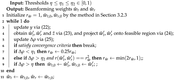
  To transform the linearized problem in (21) into a convex optimization problem, we use an additional variable z and relax the constraints C1 and C2. Specifically, the linearized problem is rewritten as

$$\begin{array}{ccc}\hfill & \underset{{\tilde{\mathit{w}}}_t,{\tilde{\mathit{w}}}_r,z}{max}z\hfill & \\ \mathrm{s}.\mathrm{t}.\hfill & \hfill & \\ \mathrm{C}1:\hfill & {\tilde{w}}_{tm,u}^{*}{\tilde{w}}_{tm,u}\le P_{max},\hfill & \forall m,u,\hfill \\ \mathrm{C}2:\hfill & {\tilde{\mathit{w}}}_{rn}^H{\tilde{\mathit{w}}}_{rn}\le 1,\hfill & \forall n\hfill \\ \mathrm{C}3:\hfill & {\overline{\mathcal{N}}}_{k,m,n}-y{\overline{\mathcal{D}}}_{k,m,n}\ge z,\hfill & \forall k,m,n\hfill \\ \mathrm{C}4:\hfill & r({\tilde{\mathit{w}}}_t,{\tilde{\mathit{w}}}_r)\le r_{\tilde{\mathit{w}}}^2.\hfill & \end{array}$$

(23)

with

$$r({\tilde{\mathit{w}}}_t,{\tilde{\mathit{w}}}_r)={\sum }_m\parallel {\tilde{\mathit{w}}}_{tm}-{\tilde{\mathit{w}}}_{tm,0}{\parallel }^2/\parallel {\tilde{\mathit{w}}}_{tm,0}{\parallel }^2+{\sum }_n\parallel {\tilde{\mathit{w}}}_{rn}-{\tilde{\mathit{w}}}_{rn,0}{\parallel }^2/{\parallel {\tilde{\mathit{w}}}_{rn,0}\parallel }^2\le r_{\tilde{\mathit{w}}}^2.$$

The constraint C4, based on the trust region [31], is designed to ensure that the solution is also suitable for the original problem in (17). This convex problem can be effectively addressed by specialized convex optimization toolboxes, such as CVX, YALMIP, or Mosek. Let $\{{\widehat{\mathit{w}}}_t,{\widehat{\mathit{w}}}_r,\widehat{z}\}$ denote the obtained solution. The solution should be projected onto the feasible region of the original problem. For the mth transmit node and the nth receive node, the projection process is

$$\begin{array}{cc}\hfill & {\widehat{\mathit{w}}}_{tm}\leftarrow \sqrt{P_{max}}exp\{j\angle {\widehat{\mathit{w}}}_{tm}\},\hfill \\ \hfill & {\widehat{\mathit{w}}}_{rm}\leftarrow {\widehat{\mathit{w}}}_{rm}/\parallel {\widehat{\mathit{w}}}_{rm}\parallel .\hfill \end{array}$$

(24)

To evaluate the actual increase in the minimum value of SCNRs, we define a ratio

$$\Delta \rho =min\{{\mathcal{N}}_{k,m,n}({\widehat{\mathit{w}}}_{tm},{\widehat{\mathit{w}}}_{rn})-y{\mathcal{D}}_{k,m,n}({\widehat{\mathit{w}}}_{tm},{\widehat{\mathit{w}}}_{rn})\}/\widehat{z}.$$

(25)

If $\Delta \rho$ is positive and large enough, rebuild the problem in (23) by using the solution as the new expansion point; otherwise, reduce the value of $r_{\tilde{\mathit{w}}}$ in C4 and then reoptimize the problem. Iterate these two steps until one of the following convergence criteria is satisfied:

• $\widehat{z}<0$ or $|r_{\tilde{\mathit{w}}}|\le \epsilon$.
• The iteration count has reached its maximum value.

where $\epsilon$ is a small enough positive constant. The whole process of the successive convex approximation (SCA)-based method for the first stage is given in Algorithm 1. In this paper, we set $\eta =0$, ${\eta }_1=0.25$, and ${\eta }_2=0.75$.

Algorithm 1: SCA-based method for the optimization of beamforming weights

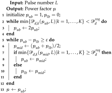
3.2.6. Optimization of Transmit Power and Pulse Number

This stage optimizes the transmit power of the transmit nodes and the pulse number. To keep the balance of SCNRs in all transmit–receive channels, a uniform power factor is set for all transmit nodes, i.e., transmit nodes share a power factor and have equal transmit power. Therefore, the objective in (14) is equivalent to minimizing the power factor. For a given power factor $\mathcal{p}\in (0,1]$, the actual power of the mth transmit node is

$$P_{tm}=\mathcal{p}{\widehat{\mathit{w}}}_{tm}^H{\widehat{\mathit{w}}}_{tm}=\mathcal{p}{P}_{max}U,$$

(26)

where $m=1,\dots ,M$. Multiplied by the square root of the power factor, the transmit beamforming weight vectors are scaled down to

$${\tilde{\mathcal{w}}}_t=\sqrt{\mathcal{p}}{\widehat{\mathit{w}}}_t.$$

Then, the observation area generation problem in (15) can be written as

$$\begin{array}{cc}\hfill & \underset{\mathcal{p},L}{min}L\hfill \\ \hfill & \underset{\mathcal{p},L}{min}\mathcal{p}\hfill \\ \hfill & \mathrm{s}.\mathrm{t}.\hfill \\ \hfill & {\mathcal{P}}_{d,k}(\mathcal{p},L|{\widehat{\mathit{w}}}_t,{\widehat{\mathit{w}}}_r,\theta ,{\mathcal{P}}_{fa})\ge {\mathcal{P}}_d^{req},\forall k,\hfill \\ \hfill & L\le L_{max},L\in {\mathbb{Z}}^{+},\hfill \\ \hfill & \mathcal{p}\in (0,1],\hfill \end{array}$$

(27)

where ${\widehat{\mathit{w}}}_t$ and ${\widehat{\mathit{w}}}_r$ are the transmit and receive beamforming weight vectors, which are determined at the first stage. Obviously, it is difficult to derive an analytical expression from (12), which describes the relationship between the detection probability and these two parameters $\mathcal{p}$ and L. Fortunately, increasing the transmit power or the pulse number will improve or at least maintain the detection probability, while all other conditions remain constant. Based on this monotonicity, we can determine the optimal power factor for a specified pulse number by a binary search, whose process is shown in Algorithm 2. Therefore, by repeating this search process, the optimal power factors for all feasible pulse numbers will be obtained. We can construct a Pareto solution set for the problem in (27) by integrating all feasible solutions, i.e., their power factors are less than 1. By combining these two stages, the process of our method is given in Algorithm 3. To control the number of loops, we set $L_{max}=20$.

Algorithm 2: Binary search for optimization of transmit power and pulse number

Algorithm 3: Summary of the proposed method

3.2.7. Time Complexity

The original form of the observation area generation problem in (15) contains two types of decision variables: the transmit–receive beamforming complex weights and the pulse number. Their total dimension is $2(M+N)U+1$. Hence, with the grid consisting of $N_s$ points in each dimension, the time complexity of the grid search method is

$$\mathcal{O}\left(N_s^{2(M+N)U+1}\right).$$

Our proposed method has two stages. In the first stage, each iteration utilizes the interior point method to solve a convex programming problem in (23). This problem has $(M+N)U$ complex variables, a real variable, and $KMN+N+MU+1$ constraints. In each iteration, the time complexity is

$${\mathcal{O}}_1(N_{c1}{N}_{v1}^3+N_{c1}^2{N}_{v1}^2+N_{c1}^3+N_{v1}^3),$$

with

$$\begin{array}{cc}\hfill N_{c1}& =KMN+N+MU+1,\hfill \\ \hfill N_{v1}& =2(M+N)U+1.\hfill \end{array}$$

For each feasible pulse number, the time complexity of the binary search in the second stage is ${\mathcal{O}}_2(log(1/\epsilon ))$, determined by the precision $\epsilon$. Thus, the time complexity of the second stage is ${\mathcal{O}}_2(L_{max}log(1/\epsilon ))$. The total time complexity of the proposed method is $I_1{\mathcal{O}}_1+{\mathcal{O}}_2$, where $I_1$ is the maximum iterations of the first stages. The time complexity of the grid search method has an exponential relationship with $2(M+N)U+1$. When $(M+N)U$ is large, the proposed method has a lower time complexity compared to the grid search method.

4. Simulation Result and Analysis

We analyze a 4 × 4 distributed phased MIMO radar system under two node placement schemes, uniform and random, as shown in Figure 5. There is a surveillance region that has been divided into multiple CUTs. In the ground coordinate system, this surveillance region has an azimuth angle range of −35° to 35°, a horizontal distance range to the origin of 6 to 12 km, and a height range of 3 to 9 km. To fully cover the surveillance region, 205 cubic observation areas are arranged as shown in Figure 6. Other parameters of the system model are given in

Table 2. The basic parameters.

NODE	Symbol	Meaning	Value
	$U_{col}$	element number in column	10
	$U_{row}$	element number in row	10
	U	total element number	100
	${\vartheta }_{3dB,★}$	3 dB beam width in elevation	180°
	${\phi }_{3dB,★}$	3 dB beam width in azimuth	180°
	$P_{max}$	element maximum transmit power	50 W
	$f_c$	carrier frequency	1 GHz
	$T_{PRI}$	pulse repetition interval	1 ms
	$\mathcal{L}$	system loss	4 dB
	$B_{\tilde{\mathit{n}}}$	noise bandwidth	0.5 MHz
TARGET	Symbol	Meaning	Value
	$v_{min}$	minimum velocity	170 km/h
	$v_{max}$	maximum velocity	1080 km/h
	${\sigma }_{min}^2$	minimum RCS	1 m2
	$r_{size}$	target size	1 m
OTHERS	Symbol	Meaning	Value
	$\Delta \theta$	angle interval of clutter surfaces	5°
	$\Delta ϵ$	edge length of CUTs	300 m
	$v_{wind}$	wind speed	1.25 m/h
	${\mathcal{P}}_d^{req}$	threshold of detection performance	0.9
	${\mathcal{P}}_{fa}$	false alarm probability	1 × 10−6
	${\gamma }_0$	normalized reflectivity parameter	1

. In early warning scenarios, the emphasis is on the rapid detection and identification of potential threats rather than the precise localization of targets. The low range resolution is typically enough. Hence, we set the signal bandwidth $B_{band}$ to 0.5 MHz, and the edge length of the CUTs can be approximated by $\Delta ϵ=c/\left(2B_{band}\right)$ = 300 m. To simplify the analysis, the noise bandwidth is equal to the signal bandwidth. In addition, the system loss for each channel is set to an identical value, i.e., ${\mathcal{L}}_{k,m,n}={\mathcal{L}}_{k,b,m,n}=\mathcal{L}$.

We then provide the calculation methods for target echo covariance and ground clutter covariance. The covariance of matched filter output of target echoes is given by

$$\mathbb{E}\left({\tilde{y}}_{k,m,n,\ell }{\tilde{y}}_{k,m^{\prime },n^{\prime },{\ell }^{\prime }}^{*}\right)={\displaystyle \frac{1}{V}}{\tilde{a}}_{k,m,n}{h}_{k,m,n}{\tilde{a}}_{k,m^{\prime },n^{\prime }}^{*}{h}_{k,m^{\prime },n^{\prime }}{\beta }_{k,m,n,\ell }{\beta }_{k,m^{\prime },n^{\prime },{\ell }^{\prime }}^{*}{\mathcal{I}}_{m,n,m^{\prime },n^{\prime }},$$

with

$$\begin{array}{cc}\hfill & {\beta }_{k,m,n,\ell }=exp\left\{j{\displaystyle \frac{2\pi }{\lambda }}(v_{m,n}\ell T_{PRI}-(r_{tm}+r_{rn}))\right\},\hfill \\ \hfill & {\mathcal{I}}_{m,n,m^{\prime },n^{\prime }}=4\pi \left({\displaystyle \frac{sin\left(D_{m,n,m^{\prime },n^{\prime }}{r}_{size}\right)}{{\left(D_{m,n,m^{\prime },n^{\prime }}\right)}^3}}-{\displaystyle \frac{r_{size}cos\left(D_{m,n,m^{\prime },n^{\prime }}{r}_{size}\right)}{{\left(D_{m,n,m^{\prime },n^{\prime }}\right)}^2}}\right),\hfill \\ \hfill & {\mathcal{A}}_{m,n}={\displaystyle \frac{2\pi }{\lambda }}(cos{\theta }_{tm}cos{\varphi }_{tm}+cos{\theta }_{rn}cos{\varphi }_{rn}),\hfill \\ \hfill & {\mathcal{B}}_{m,n}={\displaystyle \frac{2\pi }{\lambda }}(sin{\theta }_{tm}cos{\varphi }_{tm}+sin{\theta }_{rn}cos{\varphi }_{rn}),\hfill \\ \hfill & {\mathcal{C}}_{m,n}={\displaystyle \frac{2\pi }{\lambda }}(sin{\varphi }_{tm}+sin{\varphi }_{rn}),\hfill \\ \hfill & D_{m,n,m^{\prime },n^{\prime }}^2={({\mathcal{A}}_{m,n}-{\mathcal{A}}_{m^{\prime },n^{\prime }})}^2+{({\mathcal{B}}_{m,n}-{\mathcal{B}}_{m^{\prime },n^{\prime }})}^2+{({\mathcal{C}}_{m,n}-{\mathcal{C}}_{m^{\prime },n^{\prime }})}^2,\hfill \end{array}$$

where $({\theta }_{★},{\varphi }_{★},r_{★})$ are the spherical coordinates of the nodes in the target coordinate system, $★=tm,rn$. These coordinates can be obtained by setting the origin of the target coordinate system at the center of the CUT. The details of the derivation can be found in Appendix A. We can find that the target echo covariance is influenced by the target velocity, size, node location, and sampling time.

Internal motion, such as the tree leaves swaying in the wind, causes clutter decorrelation in time. According to the Billingsley model [46], the covariance of matched filter output of clutter echoes is given by

$$\mathbb{E}\left({\tilde{c}}_{k,m,n,\ell }{\tilde{c}}_{k,m,n,{\ell }^{\prime }}^{*}\right)={\sigma }_{\tilde{\mathbf{c}},k,m,n}^2·\left({\displaystyle \frac{{\alpha }_0}{{\alpha }_0+1}}+{\displaystyle \frac{1}{{\alpha }_0+1}}{\displaystyle \frac{{\left({\beta }_0\lambda \right)}^2}{{\left({\beta }_0\lambda \right)}^2+{\left(4\pi {\tau }_{\ell ,{\ell }^{\prime }}\right)}^2}}\right),$$

with

$$\begin{array}{cc}\hfill & {\alpha }_0=489.8v_w^{-1.55}{f}_c^{-1.21},\hfill \\ \hfill & {\beta }_0=0.1048({log}_{10}{v}_w+0.4147),\hfill \\ \hfill & {\sigma }_{\tilde{\mathbf{c}},k,m,n}^2=\sum _{b=1}^B{\parallel {\tilde{a}}_{k,b,m,n}{h}_{k,b,m,n}\parallel }^2,\hfill \\ \hfill & {\tau }_{\ell ,{\ell }^{\prime }}=|\ell -{\ell }^{\prime }|T_{PRI}.\hfill \end{array}$$

where $v_w$ is the wind speed in statute miles per hour.

4.1. Influence of Initial Beamforming Weights

In this subsection, we evaluate the influence of initial beamforming weights on the optimization method for beamforming weights, as outlined in Section 3.2.5. We compare two methods for selecting initial beamforming weights. One is the method we propose in Section 3.2.3. The other is a conventional method that uses a predefined set of weights to steer the beam in a specific direction. We select an observation area with its center defined by ${\mathbf{X}}_c=[7050,-3150,3600]$ m in the ground coordinate system. Using (1) and (2), we obtain the steering vectors denoted by ${\tilde{\mathit{\alpha }}}_{c,★}$, where $★=tm,rn$. Note that the initial beamforming weights should satisfy the constraints in (17). To achieve full transmit power, the initial beamforming weight vector for the mth transmit node is calculated as ${\tilde{\mathit{w}}}_{tm,0}=\sqrt{P_{max}}exp\{j\angle {\tilde{\mathit{\alpha }}}_{c,tm}\}$. Similarly, the initial beamforming weight vector for the nth receive node is determined through normalization: ${\tilde{\mathit{w}}}_{rn,0}={\tilde{\mathit{\alpha }}}_{c,rn}/\parallel {\tilde{\mathit{\alpha }}}_{c,rn}\parallel$. These weight vectors allow each node to direct its beam towards the observation area.

Figure 7 illustrates the initial and optimized results of SCNRs in a channel at each CUT within the observation area. We can find that all SCNRs have improved. The results of different initial value methods differ greatly under the uniform node placement scheme. Compared to conventional beamforming weights, the initial weights obtained through our proposed method lead to a more balanced result. The mean SCNR has seen at least a 10.45 dB improvement. Furthermore, the SCNR range has been significantly condensed, with its maximum interval reduced from 19.51 to 10.89 dB. However, when conventional beamforming weights are used, the corresponding improvement is only 6.37 dB, and the SCNR range is narrowed from 36.61 to 27.19 dB. Under the random node placement scheme, the results from different initial value methods are essentially the same. The mean SCNR shows an improvement of at least 13.90 dB, and the range of SCNR values has been reduced from 13.55 to 8.02 dB.

The failure of the conventional beamforming method arises because the required beam width for a node is not constant; it varies with the distance from the node to the observation area and is influenced by the size of the observation area. However, the conventional beamforming method produces a fixed beam width, making it difficult to consistently satisfy the varying requirements of the nodes. Figure 8 shows the antenna radiation pattern of the node closest to the observation area. It can be found that the beam width formed by the conventional beamforming method is too narrow to cover the selected observation area under the uniform node placement scheme. For CUTs within the observation area, the difference in antenna beam power is greater than 28 dB. Using our proposed method, the difference can be reduced to less than 5 dB. Under the random node placement scheme, the node is far enough from the observation area. We can find that these two methods are equivalent, which can be easily proven by setting $d\to +\infty$ in (19). The final differences are both less than 7 dB.

The above results demonstrate a significant sensitivity of our beamforming weight optimization method to the selected initial beamforming weights. However, by employing our method for selecting initial beamforming weights, we can ensure convergence to an acceptable suboptimal solution.

4.2. Influence of Pulse Number

This subsection evaluates the influence of the pulse number on the power factor and the coverage of observation area. Figure 9 shows the power factor obtained with different pulse numbers. The power factor represents the scaling of the transmit power. The actual transmit power of the nodes is the product of the maximum power of the elements, the specified power factor, and the number of elements. It can be found that, without sacrificing detection performance, the required transmit power is reduced by increasing the pulse number. However, it is important to note that this relationship is not linear; as the pulse number increases, the decrease in transmit power becomes less significant. In practice, considering the energy utilization efficiency of our system, we can select the optimal pulse number that minimizes energy consumption. Furthermore, the logarithm of the feasible power factors should be less than 0. This limitation makes the effective range of pulse numbers for these two node placement schemes both begin at 3.

Next, we use the Intersection over Union (IoU) as the evaluation metric. The IoU measures the overlapping volume between the predefined and generated observation areas relative to their total volume. The higher the IoU value, the closer the generated observation area is to the predefined one. Figure 10 shows the generated observation areas with pulse numbers of 3, 5, and 7. Under the uniform node placement scheme, the IoU is stable at around 0.38 with power factors of 0.77, 0.41, and 0.29. Under the random node placement scheme, the IoU is stable at around 0.24 with power factors of 0.70, 0.40, and 0.29. The coverage of the generated observation area is consistent and is capable of completely covering the predetermined observation area. The low IoU suggests that cubic observation areas may not be optimal in terms of energy utilization efficiency. However, the regular shape will facilitate the arrangement of observation areas in a surveillance region.

4.3. Influence of Observation Area Locations

This subsection evaluates the influence of observation area locations on the required time resources and the energy utilization efficiency. The minimum pulse number required in each observation area is shown in Figure 11. These two node placement schemes result in total pulse numbers of 756 and 811, respectively, which are below the upper bound of pulse number $L_{max}\approx \Delta ϵ/\left(v_{max}{T}_{PRI}\right)=1000$. This ensures that a target can be observed once before it crosses a CUT. In general, as the distance between the observation areas and the radar system increases, so does the required number of pulses. This occurs because the area of clutter belts expands with increasing distance. This expansion leads to a decrease in SCNR, which requires an increase in pulses to maintain radar detection capability.

Figure 12 shows five generated observation areas in different locations. We observe that the directionality of the generated observation areas intensifies as the distance increases, with their boundaries evolving from a roughly spherical shape to an ellipsoidal one. The IoU reduces from 0.49 to 0.29 for the uniform node placement scheme, and from 0.29 to 0.18 for the random node placement scheme. Although a uniformly aligned arrangement of observation areas is simple, it comes at the cost of reduced energy utilization efficiency. This trade-off between the convenience of the observation area arrangement and the efficiency of radar energy utilization brings high challenges to the design and arrangement of observation areas.

To further validate the effectiveness of our proposed method, a comparison was made with a monostatic phased array radar system. The monostatic phased array radar can be built by setting the number of nodes M, N to 1, the number of elements U to 20 × 20 and reducing the placement radius to 0. According to the empirical formula, the azimuth and elevation beam width of this phased array radar are equal to 5° [17]. To fully cover the surveillance region, 120 beam positions are required. The pulse number assigned to each beam position is $L_{max}$/120 ≈ 8. The detection performance of each CUT is calculated separately. For the kth CUT, the beamforming weights are determined by the corresponding steering vector in (2) as

$$\begin{array}{cc}\hfill & {\tilde{\mathit{w}}}_{tm}=\sqrt{P_{max}}{\tilde{\mathit{\alpha }}}_{k,tm},\hfill \\ \hfill & {\tilde{\mathit{w}}}_{rn}=W_{Cheb}\odot {\tilde{\mathit{\alpha }}}_{k,rn}/\parallel W_{Cheb}\odot {\tilde{\mathit{\alpha }}}_{k,rn}\parallel ,\hfill \end{array}$$

where $W_{Cheb}$ is a 2D Chebyshev window with side-lobe attenuation 40 dB. ⊙ is the operation of element-wise multiplication. Under these parameters, the time and power resources are fully utilized for the phased array radar. Figure 13 shows the detection performance of CUTs located at different heights. It can be found that the phased array radar exhibits non-uniform detection performance in the surveillance region. The detection probability decreases significantly with increasing distance from the radar. Moreover, even the maximum value of the detection probability is considerably lower than the desired threshold of 0.9. In contrast, distributed phased MIMO radars that adopted different node placement schemes are capable of providing the required detection performance, as shown in Figure 13b,c. Although detection performance is also affected by the location of CUTs, the performance differences over the surveillance region are relatively small. Uniform detection performance in different CUTs minimizes the risk of missing potential threats due to variations in position.

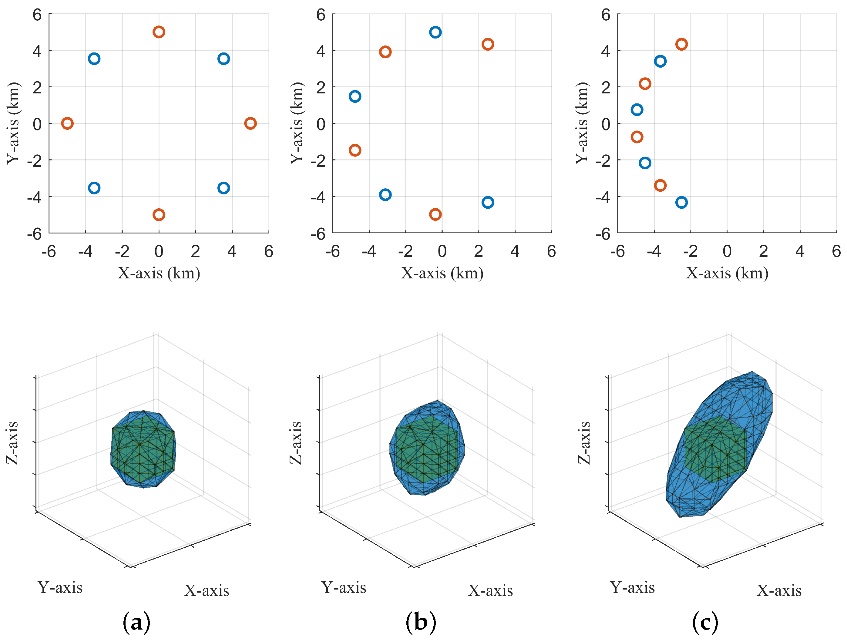
4.4. Influence of Node Location

In this subsection, we compare the effects of node placement on the energy utilization efficiency. All nodes are evenly located on an arc. The center of an observation area is located at [0, 0, 5000] m. This geometric relationship effectively eliminates the variability introduced by the distance differences between the nodes and the observation area. Figure 14 shows the generated observation area with various node placements. We find that as the angle range of placement decreases, the IoU gradually reduces from 0.69 to 0.31, while the pulse number or the power factor increases to some extent. When the placement angle of the nodes is limited in a narrow range, the generated observation area exhibits enhanced directivity. This is attributed to the similarity in the direction of energy radiation from the nodes towards the observation area. In contrast, as the placement angle widens, it leads to a reduction in directivity. The mismatch between the shape of the predefined observation area and the geometric distribution of the nodes can result in wasted beam energy, which affects the radar detection efficiency. This is also indicated by the results in Section 4.3. When using cubic observation areas, the uniform node placement scheme results in lower energy wastage. Specifically, the observation areas have a higher IoU value with a lower pulse number requirement.

5. Discussion

5.1. The Effectiveness of the Balanced SCNR Strategy

In our method, the balanced SCNR strategy is the key to solving the observation area generation problem. This strategy aims to enhance the overall detection capability of observation areas and ensure that no single channel or CUT dominates. The result of Figure 7 has shown that the balanced SCNR strategy significantly improves the mean SCNR and reduces the SCNR range for all CUTs in the observation area. This effect reflects a more effective utilization of radar resources, contributing to a more reliable target detection, even in the presence of clutter and noise. This reliability is also reflected in the fact that the coverage of the generated observation area hardly changes with the transmit power and the pulse number, which is shown in Figure 10. Compared to monostatic phased radars, the detection capability of distributed phased MIMO radars is no longer affected by the distance to targets, as shown in Figure 13. Therefore, without compromising detection performance, distributed phased MIMO radars can reduce transmit power to increase node survivability and operational time, or increase transmit power in exchange for time to perform other radar tasks. The balanced SCNR strategy not only enhances the fault tolerance of the system but also allows greater scalability and flexibility in dynamic environments. However, we only verified the effectiveness of this strategy under centralized processing. To accommodate the situation of limited communication resources, it is necessary to further verify its effectiveness under decentralized processing [47,48].

5.2. A Trade-Off between Beam Energy Utilization Efficiency and Scheduling Convenience

The ability to shape observation areas is affected by geometric relationships, as shown in Figure 12 and Figure 14. The generated observation areas are not precisely aligned with the predefined areas, resulting in a lower IoU value. This difference is particularly obvious when the observation area is far from the radar system and the angle range of node placement is limited.

The fundamental reasons of this result is multifaceted. Firstly, the geometry of the nodes and the shape of the observation areas do not match. Secondly, the distribution and intensity of the clutter vary with different distances. Finally, phased array antennas have limitations in adjusting the beam width, as shown in Figure 8. It is difficult to achieve perfect coverage of the observation area. To enhance beam energy utilization efficiency, it is essential to design a suitable shape for observation areas. However, an overly complex shape will cause difficulties in observation area arrangement and increase the complexity of beam scheduling.

6. Conclusions

In this paper, we proposed a method for distributed phased MIMO radars to actively generate a predefined observation area by optimizing the beamforming weights and beam dwell time. This method constructs a Pareto solution set, balancing radar detection efficiency and survivability while ensuring that the radar can provide an acceptable detection capability within the observation area. Although this method does not give an optimal resource management scheme for early warning scenarios, it can be used to construct a structured early warning framework for resource management.

Simulations reveal that the proposed method can efficiently generate a predefined observation area in a wide region. By uniformly arranging observation areas with regular shapes to cover the surveillance area, radar systems can achieve the early warning function without the need to focus on the specific details of beam scheduling. However, some limitations of the method have also been revealed. In particular, the ability to generate observation areas is significantly influenced by the geometric relationship between nodes and observation areas. To obtain a high utilization efficiency of beam energy, a more refined design of the observation area shape is needed in applications. Future work will focus on optimizing the design of observation areas, including the shape, performance threshold, and location arrangement.

References

1. Fishler, E.; Haimovich, A.; Blum, R.; Cimini, L.; Chizhik, D.; Valenzuela, R. Spatial diversity in radars-models and detection performance. IEEE Trans. Signal Process. 2006, 54, 823–838. [Google Scholar] [CrossRef]
2. Haimovich, A.M.; Blum, R.S.; Cimini, L.J. MIMO radar with widely separated antennas. IEEE Signal Process. Mag. 2008, 25, 116–129. [Google Scholar] [CrossRef]
3. Aittomaki, T.; Koivunen, V. Performance of MIMO radar with angular diversity under swerling. IEEE J. Sel. Top. Signal Process. 2010, 4, 101–114. [Google Scholar] [CrossRef]
4. Qi, C.; Xie, J.; Zhang, H.; Ding, Z.; Yang, X. Optimal configuration of array elements for hybrid distributed PA-MIMO radar system based on target detection. Remote Sens. 2022, 14, 4129. [Google Scholar] [CrossRef]
5. Sadeghi, M.; Behnia, F.; Amiri, R.; Farina, A. Target localization geometry gain in distributed MIMO Radar. IEEE Trans. Signal Process. 2021, 69, 1642–1652. [Google Scholar] [CrossRef]
6. Rabideau, D.; Parker, P. Ubiquitous MIMO multifunction digital array radar. In Proceedings of the Thrity-Seventh Asilomar Conference on Signals, Systems & Computers, Pacific Grove, CA, USA, 9–12 November 2003; pp. 1057–1064. [Google Scholar]
7. Luo, D.; Wen, G.; Liang, Y.; Zhu, L.; Song, H. Beam scheduling for early warning with distributed MIMO radars. IEEE Trans. Aerosp. Electron. Syst. 2023, 59, 6044–6058. [Google Scholar] [CrossRef]
8. Chen, H.; Ta, S.; Sun, B. Cooperative game approach to power allocation for target tracking in distributed MIMO radar sensor networks. IEEE Syst. J. 2015, 15, 5423–5432. [Google Scholar] [CrossRef]
9. Zhang, H.; Liu, W.; Xie, J.; Zhang, Z.; Lu, W. Joint subarray selection and power allocation for cognitive target tracking in large-scale MIMO radar networks. IEEE Syst. J. 2020, 14, 2569–2580. [Google Scholar] [CrossRef]
10. Zhang, H.; Liu, W.; Zhang, Z.; Lu, W.; Xie, J. Joint target assignment and power allocation in multiple distributed MIMO radar networks. IEEE Syst. J. 2021, 15, 694–704. [Google Scholar] [CrossRef]
11. Lu, X.; Yi, W.; Kong, L. LPI-Based transmit resource scheduling for target tracking with distributed MIMO radar systems. IEEE Trans. Veh. 2023, 72, 14230–14244. [Google Scholar] [CrossRef]
12. Liang, Y.; Wen, G.; Zhu, L.; Luo, D.; Song, H. Detection power of a distributed MIMO radar system. IEEE Trans. Aerosp. Electron. Syst. 2023, 59, 3463–3479. [Google Scholar] [CrossRef]
13. Richards, M.A. Fundamentals of Radar Signal Processing; McGraw-Hill: New York, NY, USA, 2009. [Google Scholar]
14. Fielding, J.E. Beam overlap impact on phased-array target detection. IEEE Trans. Aerosp. Electron. Syst. 1993, 29, 404–411. [Google Scholar] [CrossRef]
15. Lu, J.; Hu, W.; Xiao, H.; Yu, W. Novel cued search strategy based on information gain for phased array radar. J. Syst. Eng. Electron. 2008, 19, 292–297. [Google Scholar]
16. Hansen, R.C. Phased Array Antennas; John Wiley & Sons: Hoboken, NJ, USA, 2009. [Google Scholar]
17. Mailloux, R.J. Phased Array Antenna Handbook; Artech House: Norwood, MA, USA, 2018. [Google Scholar]
18. Wang, H.; Xu, L.; Yan, Z.; Gulliver, T.A. Low complexity MIMO-FBMC sparse channel parameter estimate for industrial big data communications. IEEE Trans. Ind. Informat. 2021, 17, 3422–3430. [Google Scholar] [CrossRef]
19. Wu, J.; Shi, C.; Zhang, W.; Zhou, J. Joint beamforming design and power control game for a MIMO radar system in the presence of multiple jammers. IEEE Trans. Aerosp. Electron. Syst. 2024, 60, 759–773. [Google Scholar] [CrossRef]
20. Ding, Z.; Xie, J. Joint transmit and receive beamforming for cognitive FDA-MIMO radar with moving target. IEEE Sens. J. 2021, 21, 20878–20885. [Google Scholar] [CrossRef]
21. Zhou, J.; Li, H.; Cui, W. Joint design of transmit and receive beamforming for transmit subaperturing MIMO radar. IEEE Signal Process Lett. 2019, 26, 1648–1652. [Google Scholar] [CrossRef]
22. Zhou, J.; Li, H.; Cui, W. Low-Complexity joint transmit and receive beamforming for MIMO radar with multi-targets. IEEE Signal Process Lett. 2022, 27, 1410–1414. [Google Scholar] [CrossRef]
23. Faghand, E.; Mehrshahi, E.; Ghorashi, S.A. Complexity reduction in beamforming of uniform array antennas for MIMO radars. IEEE Trans. Radar Syst. 2023, 59, 413–422. [Google Scholar] [CrossRef]
24. Huang, J.; Su, H.; Yang, Y. Robust adaptive beamforming for MIMO radar in the presence of covariance matrix estimation error and desired signal steering vector mismatch. IET Radar Sonar Navig. 2020, 14, 118–126. [Google Scholar] [CrossRef]
25. Liu, R. Transmit-Receive beamforming for distributed phased-MIMO radar system. IEEE Trans. Veh. 2022, 71, 1439–1453. [Google Scholar] [CrossRef]
26. Zhang, R.; Cheng, L.; Wang, S.; Lou, Y.; Gao, Y.; Wu, W.; Ng, D.W.K. Integrated sensing and communication with massive MIMO: A unified tensor approach for channel and target parameter estimation. IEEE Trans. Wirel. Commun. 2024, 23, 8571–8587. [Google Scholar] [CrossRef]
27. Yu, X.; Alhujaili, K.; Cui, G.; Monga, V. MIMO radar waveform design in the presence of multiple targets and practical constraints. IEEE Trans. Signal Process. 2020, 68, 1974–1989. [Google Scholar] [CrossRef]
28. Wang, X.; Guo, Y.; Wen, F. EMVS-MIMO radar with sparse Rx geometry: Tensor modeling and 2D direction finding. IEEE Trans. Aerosp. Electron. Syst. 2023, 59, 8062–8075. [Google Scholar] [CrossRef]
29. Zhou, S.; Liu, H.; Zhao, Y.; Hu, L. Target spatial and frequency scattering diversity property for diversity MIMO radar. Signal Process. 2011, 91, 269–276. [Google Scholar] [CrossRef]
30. Pola, M.; Bezousek, P.; Pidanic, J. Model comparison of bistatic radar clutter. In Proceedings of the 2013 Conference on Microwave Techniques (COMITE), Pardubice, Czech Republic, 17–18 April 2013; pp. 182–185. [Google Scholar]
31. Nocedal, J.; Wright, S.J. Numerical Optimization; Springer: New York, NY, USA, 2006. [Google Scholar]
32. Weiss, M. Synchronization of bistatic radar systems. In Proceedings of the IGARSS 2004, 2004 IEEE International Geoscience and Remote Sensing Symposium, Anchorage, AK, USA, 20–24 September 2004; pp. 1750–1753. [Google Scholar]
33. Goldstein, H.; Poole, C.P.; Safko, J.L. Classical Mechanics; Wesley: San Francisco, CA, USA, 2002. [Google Scholar]
34. Agatonović, M.; Stanković, Z.; Dončov, N.; Sit, L.; Milovanović, B.; Zwick, T. Application of artificial neural networks for efficient high-resolution 2D DOA estimation. Radioengineering 2012, 21, 1178–1186. [Google Scholar]
35. Barton, D.K. Radar Equations for Modern Radar; Artech House: Boston, MA, USA, 2013. [Google Scholar]
36. Zhang, H.; Xie, J.; Shi, J.; Zhang, Z.; Fu, X.; Zwick, T. Sensor scheduling and resource allocation in distributed MIMO radar for joint target tracking and detection. IEEE Access 2019, 7, 62387–62400. [Google Scholar] [CrossRef]
37. Bodenham, D.A.; Adams, M.N. A comparison of efficient approximations for a weighted sum of chi-squared random variables. Stat. Comput. 2016, 26, 917–928. [Google Scholar] [CrossRef]
38. Yang, S.; Yi, W.; Jakobsson, A. Multitarget detection strategy for distributed MIMO radar with widely separated antennas. IEEE Trans. Geosci. 2022, 60, 5113516. [Google Scholar] [CrossRef]
39. Radmard, M.; Chitgarha, M.M.; Majd, M.N.; Nayebi, M.M. Anenna placement and power allocation optimization in mimo detection. IEEE Trans. Aerosp. Electron. Syst. 2014, 50, 1468–1478. [Google Scholar] [CrossRef]
40. Hu, Q.; Su, H.; Zhou, S.; Liu, Z. Target detection with SNR diversity for distributed MIMO radar. In Proceedings of the 2015 IEEE Radar Conference, Johannesburg, South Africa, 27–30 October 2015; pp. 87–90. [Google Scholar]
41. Liu, H.; Zhou, S.; Su, H.; Yu, Y. Detection performance of spatial-frequency diversity MIMO radar. IEEE Trans. Aerosp. Electron. Syst. 2014, 50, 3137–3155. [Google Scholar]
42. Yang, Y.; Cui, G.; Yi, W. Distributed MIMO radar detection with channel evaluation and selection strategy. In Proceedings of the 2014 IEEE Radar Conference, Cincinnati, OH, USA, 19–23 May 2014; pp. 1214–1217. [Google Scholar]
43. Dinkelbach, W. On nonlinear fractional programming. Manag. Sci. 1967, 13, 492–498. [Google Scholar] [CrossRef]
44. Rajagopal, S. Beam broadening for phased antenna arrays using multi-beam subarrays. In Proceedings of the 2012 IEEE International Conference on Communications (ICC), Ottawa, ON, Canada, 10–15 June 2012; pp. 3637–3642. [Google Scholar]
45. Remmert, R. Theory of Complex Functions; Springer: New York, NY, USA, 1991. [Google Scholar]
46. Long, M.W. Radar Reflectivity of Land and Sea; Artech House: Boston, MA, USA, 2001. [Google Scholar]
47. Lishchenko, V.; Khudov, H.; Tahyan, K.; Sapegin, E.; Zvonko, A.; Serdiuk, O. Method of the detection quality improving by complexing of the same synchronous radars into multi-radar system. In Proceedings of the 2022 IEEE 41st International Conference on Electronics and Nanotechnology (ELNANO), Kyiv, Ukraine, 10–14 October 2022; pp. 496–499. [Google Scholar]
48. Barkat, M.; Varshney, P.K. Decentralized CFAR signal detection. IEEE Trans. Aerosp. Electron. Syst. 1989, 25, 141–149. [Google Scholar] [CrossRef]
Figure 2. Geometry in the target coordinate system.
Remotesensing 16 03052 g002
Figure 3. Geometry in a channel coordinate system.
Remotesensing 16 03052 g003
Figure 5. Geometric relationships of two node placement schemes. (a) In the ground coordinate system, all nodes are evenly spaced along a circle with a radius of 5 km and a height of 0.2 km. The angular interval between the adjacent nodes is 45°. (b) All nodes are randomly distributed inside a cylinder with a height of 0.2 km and a radius of 5 km. The boresight direction of these nodes is towards the center of the surveillance area.
Remotesensing 16 03052 g005
Figure 6. Geometric relationships of observation areas. (a) CUTs contained in the surveillance region. (b) Observation area arrangement. Observation areas are designed in the shape of a cube, with an edge length five times that of the CUTs. This means that each observation area contains 125 CUTs at most. For ease of display, observation areas are randomly colored. Observation area arrangement scheme contains 5 layers; each layer has 41 observation areas.
Remotesensing 16 03052 g006
Figure 7. The range of SCNRs in channels and their mean value. The first and second lines show the results under the uniform and random node placement schemes. (a) Using the conventional beamforming method. (b) Using our proposed method.
Remotesensing 16 03052 g007
Figure 8. The antenna radiation pattern of the closest node. The first and second lines show the results under the uniform and random node placement schemes. (a) Geometric relationships of the node. The marker of the closest node has been filled. (b) Using the conventional beamforming method. (c) Using our proposed method.
Remotesensing 16 03052 g008
Figure 9. Power factors under different pulse numbers.
Remotesensing 16 03052 g009
Figure 10. Predefined and generated observation area. (a) Under the uniform node placement scheme. (b) Under the random node placement scheme. The CUTs covered under different pulse numbers are labeled separately. The public CUTs are indicated with point markers. The unique CUTs that cover the pulse numbers 3, 5, and 7 are indicated with diamond-, cross-, and circle-shaped markers.
Remotesensing 16 03052 g010
Figure 11. The requirement of minimum pulse number for observation area arrangement. The first and second lines show the results under the uniform and random node placement schemes. The minimum pulse numbers of observation areas from the bottom layer to the top layer are shown in (ae).
Remotesensing 16 03052 g011
Figure 12. Generated and predefined observation areas in different locations. These two types of observation areas are marked with blue and green, respectively. The first and second lines show the results under the uniform and random node placement schemes. The predefined observation area centers in (ae) have consistent Y and Z coordinates, specifically, Y = −150 m and Z = 3600 m, respectively. Each area is distinguished by a unique X coordinate, ranging from 5550 to 11550 m at intervals of 1500 m. For the uniform placement scheme, the IoUs are as follows: 0.49, 0.45, 0.39, 0.33, and 0.29. The power factors are 0.86, 0.72, 0.77, 0.87, and 0.74. For the random placement scheme, the IoUs are 0.29, 0.27, 0.26, 0.22, and 0.18. The power factors are 0.90, 0.91, 0.70, 0.95, and 0.86.
Remotesensing 16 03052 g012
Figure 13. Comparison of detection performance in the surveillance region. The heights of the CUTs from the first row to the last one are 3.6, 5.4, 7.2, and 9 km. (a) Phased array radar. (b) Distributed phased MIMO radar under the uniform node placement scheme. (c) Distributed phased MIMO radar under the random node placement scheme.
Remotesensing 16 03052 g013
Figure 14. Generated observation areas under different node placements. The first line shows the node placements and the second line shows the coverage of observation areas. The transmit and receive nodes are marked with blue and red, respectively. The generated and predefined observation areas are marked with blue and green, respectively. In (ac), the angle ranges of placement are 0° to 360°, 60° to 300°, and 120° to 240°. The IoUs of these observation areas are 0.69, 0.53, and 0.31. Their pulse numbers are 2, 2, and 4. The corresponding power factors are 0.66, 0.86, and 0.73.
Remotesensing 16 03052 g014