Wildfire Threshold Detection and Progression Monitoring Using an Improved Radar Vegetation Index in California

Abstract

To address the recent increase in wildfire severity and incidence, as well as the subsequent financial and physical costs, forest managers and wildland firefighting agencies rely on remotely sensed products for better decision-making and mitigation efforts. To address the remote sensing needs of these agencies, which include high spatial resolution, immunity to atmospheric and solar illumination effects, and day/night capabilities, the use of synthetic aperture radar (SAR) is under investigation for application in current and upcoming systems for all phases of a wildfire. Focusing on the active phase, a method for monitoring wildfire activity is presented based on changes in the radar vegetation index (RVI). L-band backscatter measurements from NASA/JPL’s UAVSAR instrument are used to obtain RVI images on multiple dates during the 2020 Bobcat (located in Southern CA, USA) and Hennessey (located in Northern CA, USA) fires and the 2021 Caldor (located in the Sierra Nevada region of CA, USA) fire. Changes in the RVI between measurement dates of a single fire are then compared to indicators of fire activity such as ancillary GIS-based burn extent perimeters and the Landsat 8-based difference normalized burn ratio (dNBR). An RVI-based wildfire “burn” detector/index is then developed by thresholding the RVI change. A combination of the receiver operating characteristic (ROC) curves and F1 scores for this detector are used to derive change detection thresholds at varying spatial resolutions. Six repeat-track UAVSAR lines over the 2020 fires are used to determine appropriate threshold values, and the performance is subsequently investigated for the 2021 Caldor fire. The results show good performance for the Bobcat and Hennessey fires at 100 m resolution, with optimum probability of detections of 67.89% and 71.98%, F1 scores of 0.6865 and 0.7309, and Matthews correlation coefficients of 0.5863 and 0.6207, respectively, with an overall increase in performance for all metrics as spatial resolution becomes coarser. The results for pixels identified as “burned” compare well with other fire indicators such as soil burn severity, known progression maps, and post-fire agency publications. Good performance is also observed for the Caldor fire where the percentage of pixels identified as burned within the known fire perimeters ranges from 37.87% at ~5 m resolution to 88.02% at 500 m resolution, with a general increase in performance as spatial resolution increases. All detections for Caldor show dense collections of burned pixels within the known perimeters, while pixels identified as burned that lie outside of the know perimeters have a sparse spatial distribution similar to noise that decreases as spatial resolution is degraded. The Caldor results also align well with other fire indicators such as soil burn severity and vegetation disturbance.

1. Introduction

Wildfires are natural phenomena that play an integral role in the dynamic cycle of terrestrial ecology and support numerous environmental functions [1,2], broadly categorized as “provisioning”, “regulatory”, “cultural”, and “support” services [1]. More specifically, these services can include the restoration of deteriorating ecosystems that rely on fire [3], a reduction in future fire hazards by minimizing the large-scale accumulation of surface and canopy fuels (i.e., vegetation biomass) [4], plant and animal species diversity and propagation [5], and the promotion of vegetation competition [6].

While the natural occurrence of wildfires is expected, anthropogenic activity [7,8] has resulted in ecological disturbances that in turn have influenced the severity of wildfires and the rate of their occurrence. Any increase in wildfire activity can be extremely detrimental, leading to significant impacts such as burned acreage and property damage [8,9]. The associated costs can be substantial, with 2020 alone resulting in U.S. national wildfire suppression costs exceeding USD 1.6 billion [10,11] and physical property damages to the state of California in excess of USD 4.2 billion [12]. Other impacts can include soil quality degradation [13], decreased water quality [14], and increased levels of atmospheric pollution [8].

To address the impacts of wildfires, government and wildfire mitigation agencies such as the National Interagency Fire Center and the U.S. Forest Service implement a variety of monitoring and forecasting systems in the US [8,15]. These systems incorporate information on multiple geophysical variables such as vegetation levels, soil moisture, and meteorology as inputs to long-term fire risk prediction models and to predict the complex behaviors of active fires [15]. The National Fire Danger Rating System, for example, incorporates multiple remotely sensed environmental variables derived from space- or air-borne passive optical, hyperspectral, and infrared imagery [16,17,18]. These imaging methods also have an established history of research, highlighting their usefulness in estimating many ecological variables and natural hazard applications. This includes the use of multispectral and hyperspectral techniques to estimate the moisture content of vegetation in wetland environments, vegetation biomass, and Leaf Area Index (LAI), and even to differentiate wetland plant species [19]. One multispectral metric commonly used to estimate vegetation levels is the normalized difference vegetation index (NDVI), which has been used to monitor fire-induced disturbance using clear pre- and post-fire imagery [20] and to assess post-fire ecosystem recovery to varying degrees of success [20,21].

While the usefulness of passive optics-based imaging techniques has been proven, their effectiveness during active fire periods can be impacted by the influence of solar illumination and atmospheric occlusion due to smoke [22]. An example of potential atmospheric effects is presented in Figure 1, in which Sentinel-2 optical imagery available at 10 m spatial resolution [23,24] taken over the 2021 Caldor fire in California, USA, is contrasted with a normalized difference vegetation index (NDVI) image at 5 km spatial resolution derived from VIIRS satellite multispectral optical data on the same date [25]. The opacity effects of smoke from the actively burning Caldor fire are evident and preclude the ability to remotely sense the region of interest. To account for some of these potential atmospheric impacts, current research looks to improve on metrics like the NDVI through methods such as atmospheric correction [26]. While these methods show promise, they have inherent limitations and rely on incorporating further ancillary information. A simpler approach is the use of microwave synthetic aperture radar (SAR). The microwave backscatter measurements of SAR systems can be used to combat these effects, given the all-weather active microwave imaging capabilities of SAR, their insensitivity to solar illumination, and their ability to provide the meter-scale spatial resolutions relevant for active fire monitoring [27], as indicated by a recent U.S. Forest Service–NASA joint workshop on satellite data needs for natural resource management [28].

Many radar-based metrics, including SAR, exist to monitor ecological variables that have natural hazard applications such as soil moisture [29], vegetation water content (VWC) [30], snow water equivalent [31], and deformation due to changes in various variables such as forest structure using interferometric SAR [32]. Studies related to soil moisture indicate a wide variety of successful applications such as flood monitoring and warning [33,34] and drought predictions [35], while coherence, or the coherence index, can be used to identify earthquake-related damages and large changes in surface structure due to landslides [36]. One ecological variable that is of interest to wildfire applications and natural resource management is vegetation [28].

The vegetation combustion that fuels a wildfire is a key indicator of fire activity [37]. The decreased vegetation levels that occur as a fire progresses suggest that both the degree and extent of active burn can be identified using remote sensing methods related to monitoring vegetation properties. A method based on sensing changes in vegetation properties requires quantifying vegetation levels at multiple times as a fire progresses.

Although many potential approaches for quantifying vegetation properties from radar backscatter measurements are available such as the radar forest degradation index (RFDI) and canopy structure index (CSI) [38], the RVI [39] was chosen for use due to its many desirable attributes which include its simplicity, reduced sensitivity to geometry/topography/calibration, and high degree of sensitivity to vegetation properties [40]. In particular, the RVI is an intensity normalized cross-polarized backscatter measurement that has shown good performance in monitoring vegetation properties in past studies over highly vegetated surfaces [41] and across various platforms [42,43].

To demonstrate the potential effectiveness of SAR-based scientific products in wildfire monitoring, particularly an improved RVI, we report a change detection method with air-borne SAR measurements for monitoring the active phase of wildfires. The focus on the active phase of a wildfire’s lifecycle arises from the crucial need in this phase for identifying burning or recently burned areas as part of managing fire response and resource allocations. Three wildfires (the Bobcat and Hennessey fires of 2020 and the Caldor fire of 2021) are investigated to assess the effectiveness of the method for varying SAR spatial resolutions and across multiple fires.

2. Methods

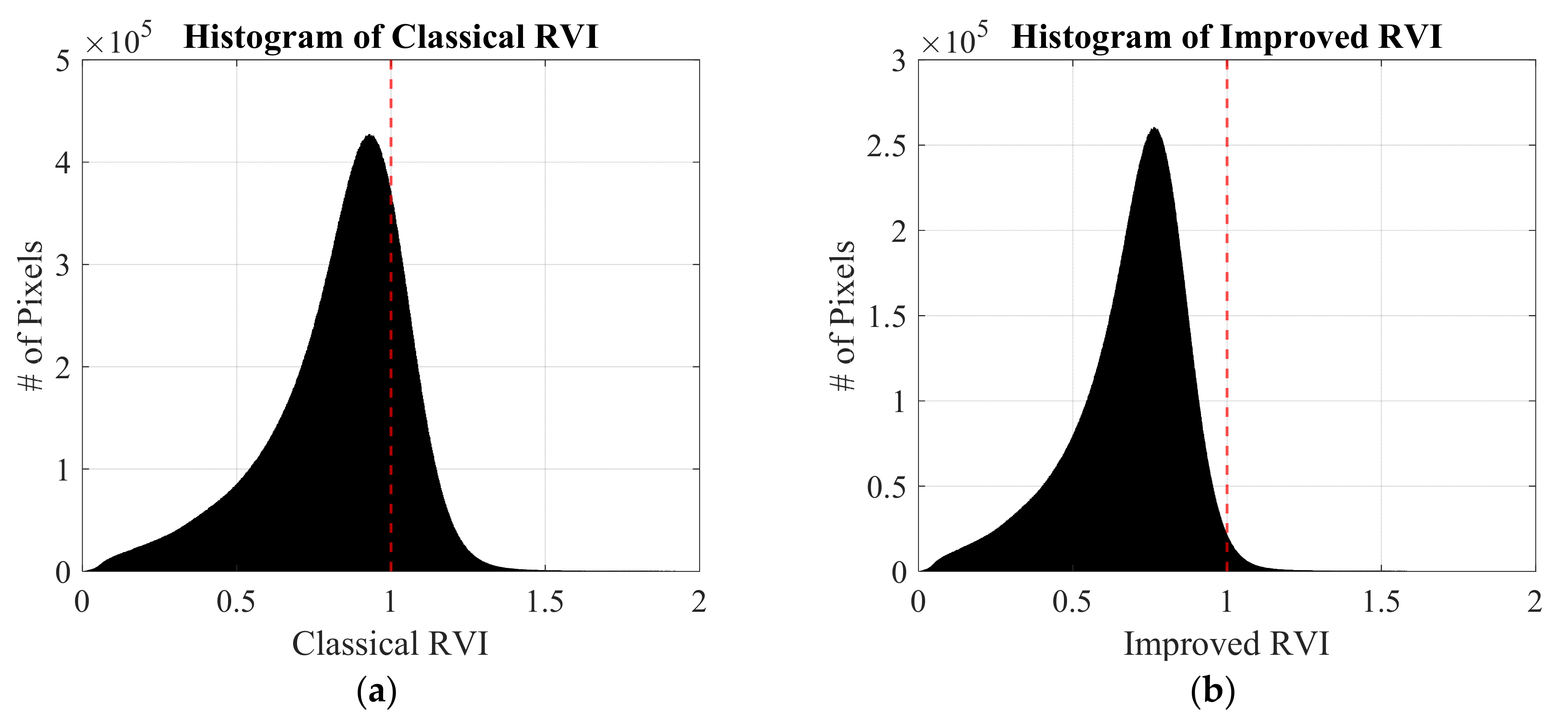
2.1. Radar Vegetation Index

The RVI is defined here as

$$\mathrm{RVI}={\displaystyle \frac{\kappa {\sigma }_{HV}}{{\sigma }_{HH}+{\sigma }_{VV}+2{\sigma }_{HV}}}$$

(1)

in which horizontally and vertically co-polarized Normalized Radar Cross-Section (NRCS) measurements are represented by ${\sigma }_{HH}$ and ${\sigma }_{VV},$ respectively, while ${\sigma }_{HV}$ represents the cross-polarized NRCS, and κ is a constant. The RVI is defined so that under certain assumptions with κ = 8 (identified as the “classical RVI”), it should range from 0 to 1, with 0 indicating bare surfaces and 1 indicating highly vegetated surfaces such as forests [39]. While this holds true for some models of vegetation scattering, it is less true in a more general sense and can lead to RVI estimates greater than 1 for many dense vegetation classes not used in developing the initial study (i.e., non-agricultural crops). Reference [44] instead proposes the use of κ = 6.57 (identified as an “improved RVI”) as applicable across a wider variety of vegetated surface conditions. Other recent RVI analyses include the development of a truncated version using Sentinel-1 [45]. One drawback in using the RVI in the form presented in equation 1 is that NRCS measurements in HH, VV, and HV polarization combinations (${\sigma }_{HH}, {\sigma }_{VV}, {\sigma }_{HV}$) are required that may not be available in all SAR observing modes, including dual, compact, or hybrid polarimetric acquisition modes (e.g., RADARSAT Constellation Mission (RCM) [46] or NASA/ISRO synthetic aperture radar (NISAR) [47]). In such cases where full polarimetry is unavailable, the use of cross-pol (HV) has shown potential for monitoring vegetation changes related to wildfire activity [48] and a dual-pol RVI is currently being investigated [49].

To analyze the potential implications of different κ pre-factors, Figure 2 illustrates histograms of the RVI from UAVSAR measurements [50] taken over the regions surrounding the three fires described in Section 3 using either κ = 8 for the “classical” RVI (left-hand column) or κ = 6.57 for the “improved” RVI (right-hand column). For the sites selected, the classical RVI method leads to large numbers of pixels with a value greater than 1, mostly for “evergreen forests” and “shrub/scrub” (i.e., non-agricultural vegetation). The results show that the use of κ = 6.57 reduces the prevalence of RVI values greater than one, making it desirable for continued analyses. The value κ = 6.57 (improved RVI) is therefore used in computing the RVI in what follows.

2.2. Change Detection Method

The change detection method developed here uses the RVI measured at two or more times during a fire’s lifecycle. The most recent RVI value minus a preceding value is then taken so that negative changes in the RVI indicate losses in vegetation. A simple threshold detection method for this change can then be applied to identify newly burned areas. To seek an appropriate detection threshold, a combination of receiver operating characteristic (ROC) curve [51,52] and F1 score [53] analyses can be used for cases in which ancillary ground truth information on the location of burned areas is available. This method (i.e., the use of the ROC curve and F1 score) was chosen for application over other statistical parameters due to its simplicity of calculation/application and “robustness” when compared to other methods [51]. Furthermore, ROC curves have been used to good effect in previous detection studies [54,55], while the F1 score has been shown to be suitable for applications to SAR [56,57,58] and other radar detection applications [59,60].

2.3. Accuracy Assessment Metrics

The ROC curve, in particular, plots the probability of detection

$$P_{detection}={\displaystyle \frac{Tru{e}_{positive}}{Tota{l}_{positive}}}$$

(2)

versus the probability of false alarm

$$P_{false alarm}={\displaystyle \frac{Fals{e}_{positive}}{Tota{l}_{negative}}}$$

(3)

as the detection threshold is varied [51]. Determining the probability of detection and the probability of false alarm requires “ground truth” reference information on both burned and unburned pixels. Ground truth information is obtained from GIS-based burn extent perimeters for the dates of radar observation [61]. Using the burn perimeters, a map is created where all pixels within the perimeter are flagged as “burned”, assuming at lease some degree of burn. Since uniform burning within the perimeter is not realistic, this information is further fine-tuned using the Landsat 8-based difference normalized burn ratio (dNBR) available at 30 m spatial resolution [62,63,64,65,66,67]. The dNBR is used to identify pixels within the burn perimeter that have been identified as experiencing very little or no degree of burn activity; such locations are then flagged as “unburned” pixels. Using the normalized burn ratio (NBR),

$$\mathrm{NBR}={\displaystyle \frac{\mathrm{NIR}-\mathrm{SWIR}}{\mathrm{NIR}+\mathrm{SWIR}}}$$

(4)

the dNBR is calculated as the difference in the NBR

$$\mathrm{dNBR}={\mathrm{NBR}}_{\mathrm{previous}}-{\mathrm{NBR}}_{\mathrm{current}}$$

(5)

of near-infrared (NIR, Landsat 8 band 5) and short-wave infrared (SWIR, Landsat 8 band 7) channels, with the most current NBR subtracted from its previous value.

This information is used to identify unburned regions when clear surface Landsat 8 imagery is available close to the same dates of investigation [67]. Given this combined ground truth information, the ROC curve provides a visual summary of the tradeoffs of the detection and false alarm probabilities versus the threshold level. A summary of the Landsat files used in this process is presented in

Table 1. Summary of Landsat files used in ground truth referencing for Bobcat and Hennessey fires.

Fire Name:	Date:	Landsat File:
Bobcat Fire	5 September 2020	LC08_L2SP_041036_20200905_20200918_02_T1
Bobcat Fire	10 October 2020	LC08_L2SP_041036_20201007_20220526_02_T1
Hennessey Fire	9 August 2020	LC08_L2SP_044033_20200809_20200918_02_T1
Hennessey Fire	12 October 2020	LC08_L2SP_044033_20201012_20201105_02_T1

.

The F1 score is defined as

$$\mathrm{F}1 \mathrm{score}={\displaystyle \frac{\mathrm{TP}}{\mathrm{TP}+\raisebox{1ex}{$1$}\!\left/ \!\raisebox{-1ex}{$2$}\right.\left(\mathrm{FP}+\mathrm{FN}\right)}}$$

(6)

where TP (true positive) is representative of correctly identified “burned” pixels, FP (false positive) is representative of incorrectly identified “burned” pixels, FN (false negative) is representative of incorrectly identified “unchanged” pixels, and TN (true negative) is representative of correctly identified “unchanged” pixels. The F1 score can be used to assess candidate threshold values given its blend of information on precision and recall [68]. In the study that follows, a threshold value that maximizes the F1 score at a given scene is considered “optimal” and used to delineate RVI change values indicative of wildfire burning.

The results reported focus on the probability of detection (P_d) and the probability of false alarm (P_fa) for the “optimal” threshold chosen by the maximum F1 score for varying spatial resolutions. Additionally, the Matthews correlation coefficient

$$\mathrm{MCC}={\displaystyle \frac{\mathrm{TP}\cdot \mathrm{TN}-\mathrm{FP}\cdot \mathrm{FN}}{\sqrt{\left(\mathrm{TP}+\mathrm{FN}\right)\left(\mathrm{TP}+\mathrm{FP}\right)\left(\mathrm{TN}+\mathrm{FP}\right)\left(\mathrm{TN}+\mathrm{FN}\right)}}},$$

(7)

indicative of the spatial correlation between ground truth reference maps and detection maps, is also reported for varying spatial resolutions [69]. The MCC typically ranges from −1 to 1, with −1 being an inversely correlated result, 0 being uncorrelated, and 1 being perfectly correlated. The inclusion of the MCC is performed to further substantiate the detection results and is chosen as it has been shown to be one of the strongest indicators of performance for binary classifications (i.e., the classification of “burned” and “unburned” pixels for this study) [70,71]. All statistical metrics are calculated using the number of burned and unburned pixels identified by these methods.

3. Description of Data

3.1. UAVSAR Data

Polarimetric L-band radar backscatter measurements from the NASA/JPL UAVSAR instrument [50,72] are used to examine the performance of the proposed change detection method. UAVSAR operates at center frequency of 1.26 GHz (~23.79 cm wavelength) and observes over a swath that spans incidence angles ranging from 25 to 65 degrees. Although the data have an original spatial resolution of approximately 0.8–1.8 m, the data are multi-looked to ~5 m resolution on an equiangular georeferenced grid to reduce speckle effects and to simplify the colocation of measurements between repeat-pass flights. A summary of the basic operating characteristics of the UAVSAR instrument is presented in

Table 2. A summary table of the radar characteristics of the UAVSAR instrument used in this study [72].

UAVSAR Characteristic	Quantity/Value
Radar Type	Synthetic Aperture Radar
Frequency	1.26 GHz
Wavelength	23.79 cm
Bandwidth	80 MHz
Polarization	Full Pol (HH, VV, HV, VH)
Swath Width	16 km
Incidence Angle	25 degrees–65 degrees
Transmit Power	3.1 kW
Altitude	2000–18,000 m
Inherent Spatial Resolution	~1.8 m
Products Used	MLC, Ground Range Projected Intensity

.

3.2. Wildfire Sites

Three major wildfire events (the 2020 Bobcat, 2020 Hennessey, and 2021 Caldor fires, see Figure 3) were identified that had repeat-pass UAVSAR overflights during the active fire period or that had one pass during the active fire period and another immediately prior to or immediately following. The three fires selected for this study focus on the state of California due to the depth and availability of wildfire-related datasets and information with which to perform comparison analyses. Additionally, the state of California provides an interesting testbed to investigate the method over different land classes as the area comprises a variety of climatological regimes over a small geographic region [73,74,75,76]. This is the case with the three fires identified for study which lie in different climatologic regions of the state. This information can be used to better understand and analyze fire detection results.

The Bobcat fire burned from 6 September to 27 November 2020 in the Angeles National Forest (Northeast of Los Angeles) in California and covered an area of approximately 115,997 acres (469 km²) [10,11,12,77]. UAVSAR repeat-track lines were flown on 18 September and 14/15 October 2020 during the active burn phase of the fire that have substantial geographic overlap with the known burn perimeters. This actively burning region during this time consists predominantly of “shrub/scrub” vegetation with intermixed areas of “evergreen forest” [78] and lies in a semi-arid region of California that receives less rainfall than the other two wildfire locations being investigated [77]. The southern and central portions of the wildfire cover a semi-mountainous region, while the northern portion covers a lower-elevation region with reduced surface height variations approaching a more desert-like area [73,74,75]. A satellite image highlighting the respective UAVSAR dates of the fire burn perimeters and a National Land Cover Database (NLCD) map are provided in Figure 4a,b. The Bobcat fire represents a scenario in which significant time has elapsed between UAVSAR measurements and in which extensive burning has occurred between the measurement dates.

The Hennessey fire burned from 17 August to 2 October 2020 near Lake Berryessa (North of San Francisco), California [10,11,79], and covered an area of approximately 305,651 acres (1237 km²) (see Figure 4c,d). Four UAVSAR repeat-track lines with substantial geographic overlap with the overall burn extent perimeter are available for 3 September and 14 October 2020. The region surrounding the Hennessey fire is predominantly classified as “shrub/scrub” and “grassland/herbaceous”, with minimal areas of evergreen forest [78], and lies in a region of northern California that receives more rainfall than the region of the Bobcat fire [73,74,75]. This region has elevation and surface variations similar to those in the semi-mountainous region of the Bobcat fire. It should be noted that the western region of the fire footprint begins to approach more low mountainous terrain, while the eastern region approaches flatter terrain and agricultural fields, as indicated by the dark brown color in Figure 4d. Overall, this region is dominated more by low vegetation and grasslands compared to the other two sites. The Hennessey fire event represents a scenario where approximately one and a half months have elapsed between UAVSAR measurements, with the overall perimeter being established by the first measurement date and with continued burning occurring between the two UAVSAR measurement dates.

The Caldor fire burned from 14 August to 21 October 2021 in the El Dorado National Forest near Lake Tahoe, CA, and covered an area of approximately 221,835 acres (898 km²) [80,81]. This fire has repeat-track UAVSAR measurements on 25 August and 31 August 2021 that overlap the full burn extent perimeter footprint (Figure 4e,f). The region surrounding the Caldor fire is dominated by evergreen forest [78] and lies at a much higher elevation than the other sites investigated. The Caldor region also receives significantly more rainfall than the other wildfire sites [73]. Overall, the area surrounding the Caldor fire is predominantly mountainous terrain and is dominated more by forested and dense vegetation classes. The wildfire approaches urbanized areas to the northeast of the fire burn perimeters near Lake Tahoe and to the far west of the imagery shown. The Caldor fire represents a scenario where less than a week has elapsed between UAVSAR measurements and fire-induced vegetation changes are expected in newly burned areas.

The multiple repeat-track UAVSAR lines of the Bobcat and Hennessey fires have minimal geographic overlap and are flown in an east–west direction, with individual repeat-track lines lying either north or south of each other. For these fires, flight lines are numbered 1 through n, with the number of the line increasing for more southerly tracks (e.g., “Bobcat Line 1” lies to the north of “Bobcat Line 2”; “Hennessey Line 1” is the northern-most line and “Hennessey Line 4” is the southern-most line for the Hennessey fire). The overall spatial footprint of each repeat-track UAVSAR flightline will be highlighted in all forthcoming imagery by a dashed black outline for reference.

4. Results and Analysis

The analysis to follow first investigates changes in the RVI as indications of vegetation loss for each wildfire. Next, an analysis of ROC curves and F1 scores for the Bobcat and Hennessey fires is presented as a method of determining an “optimal” detection threshold that is used to create wildfire detection maps. The threshold determined is then applied to the Caldor wildfire.

Calculations were performed at spatial resolutions of 5 m, 25 m, 50 m, 100 m, 200 m, and 500 m to examine the impact of the spatial resolution. These spatial resolutions are determined by resampling UAVSAR measurements from the inherent UAVSAR resolution using a simple average. Unless otherwise stated, 100 m is used as the “default” resolution in most images. A spatial resolution of 100 m matches the requirements of many of the scientific products being developed/delivered by the NASA/ISRO NISAR mission [47,82] that were determined by the associated science communities and serves to moderate the impacts of speckle and thermal noise errors while remaining sufficiently fine for use in many applications. The results can also be used to examine the viability of future ~100 m wildfire products for the NISAR mission.

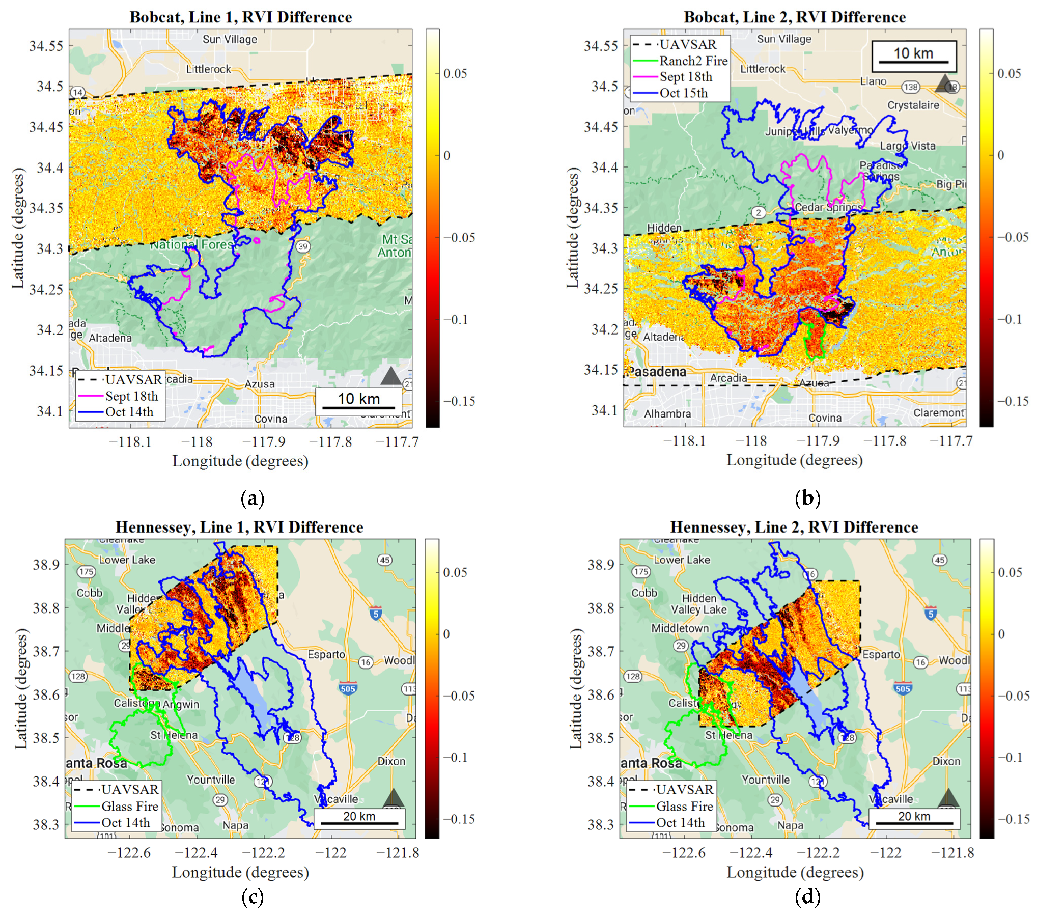
4.1. RVI Change Results

Using the calculated RVI for each UAVSAR date, the RVI change at 100 m resolution is plotted in Figure 5 for the Bobcat (Figure 5a,b), Hennessey (Figure 5c–f), and Caldor (Figure 5g) fires. The area of UAVSAR coverage is indicated with a dashed black outline, while the fire burn extent perimeters are shown as solid lines, with the applicable dates indicated in the plot legends. The outlines of other wildfires active in the area at the time of the UAVSAR measurements are also included and shown as neon green solid lines. It should be noted that any areas within the UAVSAR perimeters that do not contain information are due to UAVSAR flagging for extreme incidence angles or for inapplicable land classifications (i.e., urban areas, surface water, bare surfaces) in the NLCD [78]. This is most noticeable for the Bobcat fire (specifically Figure 5b) due to the urban areas around the city of Los Angeles. Finally, all subplots within Figure 5 are created using the same color map and scale (i.e., color bar range of RVI values) for better inter-comparison of the results. This can result in some fires having RVI changes below the largest negative change value in the color scale. Any pixels that go below the minimum scale value appear as black pixels.

The results for both lines of the Bobcat fire (Figure 5a,b) show clear correlations between the fire perimeter locations and losses (i.e., negative changes) in the RVI. The largest negative changes in the RVI are approximately −0.18 that occur in the most recently burned locations between the two perimeters.

In line 1, the largest RVI losses occur between the perimeters along the northern portion of the 14th October perimeter. The results for line 1 also show additional localized RVI losses within the original 18th September perimeter, which indicates continued burning. However, these changes are modest compared to the more drastic changes in the area between the perimeters. Line 2 also shows large losses in the RVI between the burn perimeters, with the largest ones occurring near the eastern and western edges of the two perimeters. Changes within the original perimeter are also larger than those for line 1, suggesting continued burning on a larger scale than in line 1. Furthermore, the resulting RVI changes show good agreement with outside sources of burn severity and fire classification for the Bobcat fire. This includes official thematic burn severity available through Monitoring Trends in Burn Severity (MTBS-U.S. Geologic Survey/U.S. Forest Service) [83,84], fire/burn classification using the LANDFIRE 2020 vegetation disturbance layer [85], and other sophisticated burn severity methods used for the Bobcat fire such as MODIS/ASTER burn severity/fire intensity composites [86] and other ancillary information [87].

Overall, the Bobcat results demonstrate the sensitivity of RVI changes to new burning as well as continuing burning that occurs within the one-month period between flights. The results are also able to identify negative changes in the RVI for the nearby Ranch2 fire, where a containment perimeter for the burn was established prior to the first UAVSAR date and highlights continued burning for that location.

Similar results are observed for the Hennessey fire in Figure 5c–f, with the highest degree of change again occurring within the known fire perimeter. It is noted that the Hennessey fire did not have fire burn perimeter information for both UAVSAR dates used in the analysis as minimal change in burning containment occurred, so a single perimeter (after the second flight date) is shown. Since the first UAVSAR date occurs near the establishment of the containment perimeter of the active burn period for the Hennessey fire, it will be assumed that this is a case where the burning that has occurred continued to burn up to the second UAVSAR date.

All four UAVSAR repeat-track lines show negative changes within the fire perimeter, with the largest negative changes occurring in the western perimeter areas. The eastern portions of the wildfire footprint with minimal to no change in the RVI within the fire perimeter appear visually correlated with the “grasslands” classification in Figure 4d, potentially indicating reduced RVI sensitivity to burning for this vegetation type, although a full analysis of sensitivity to particular terrain classes has not been completed at this time. Changes in the RVI are also evident within the nearby Glass fire that ignited after the first UAVSAR measurements were taken that highlights a region of new burning. Additionally, the RVI change results also show good agreement with outside sources for burn severity and classification such as the MTBS burn severity dataset [83,84], LANDFIRE 2020 vegetation disturbance “burn/fire” classification [85], and soil burn severity maps published in the official post-fire response evaluation [88].

The results for the Caldor fire in Figure 5g again show the largest changes in the RVI in areas between the perimeters for the measurement dates. The areas of largest change occur in the most western part of the burned region and in the northeast part of the most recent perimeter. The results also indicate no large-scale losses in the RVI within the 25th August perimeter. Given the 6-day time difference between UAVSAR observations of the Caldor fire, small changes in the RVI for continued burning are overshadowed by the larger changes due to new burning, which is not surprising. A comparison of Figure 5 (which uses the same color scale) further suggests that the short time between flights reduces the amount of RVI change observed for the Caldor fire. Overall, the RVI change for Caldor shows agreement with the areas of largest negative change and other fire indicators such as MTBS thematic burn severity for the region being studied during the active fire [83,84], LANDFIRE 2021 vegetation disturbance [89], and other metrics such as soil burn severity identified in the Caldor post-fire recovery framework [90].

It should be noted that the Caldor fire results in frequent positive changes in the RVI compared to the other wildfires being studied. It is possible that the mountainous terrain of the Caldor fire compared to the other wildfire sites could be the cause of this effect. Additionally, some of the largest positive changes in the RVI occur within the same small regions in which the largest negative changes occur. These effects are suspected of being caused by a change in the dominant scattering mechanism due to burning that can lead to higher backscatter from the surface due to less vegetation attenuation. Further discussion on this phenomenon is beyond the scope of this paper and is a subject for future analyses.

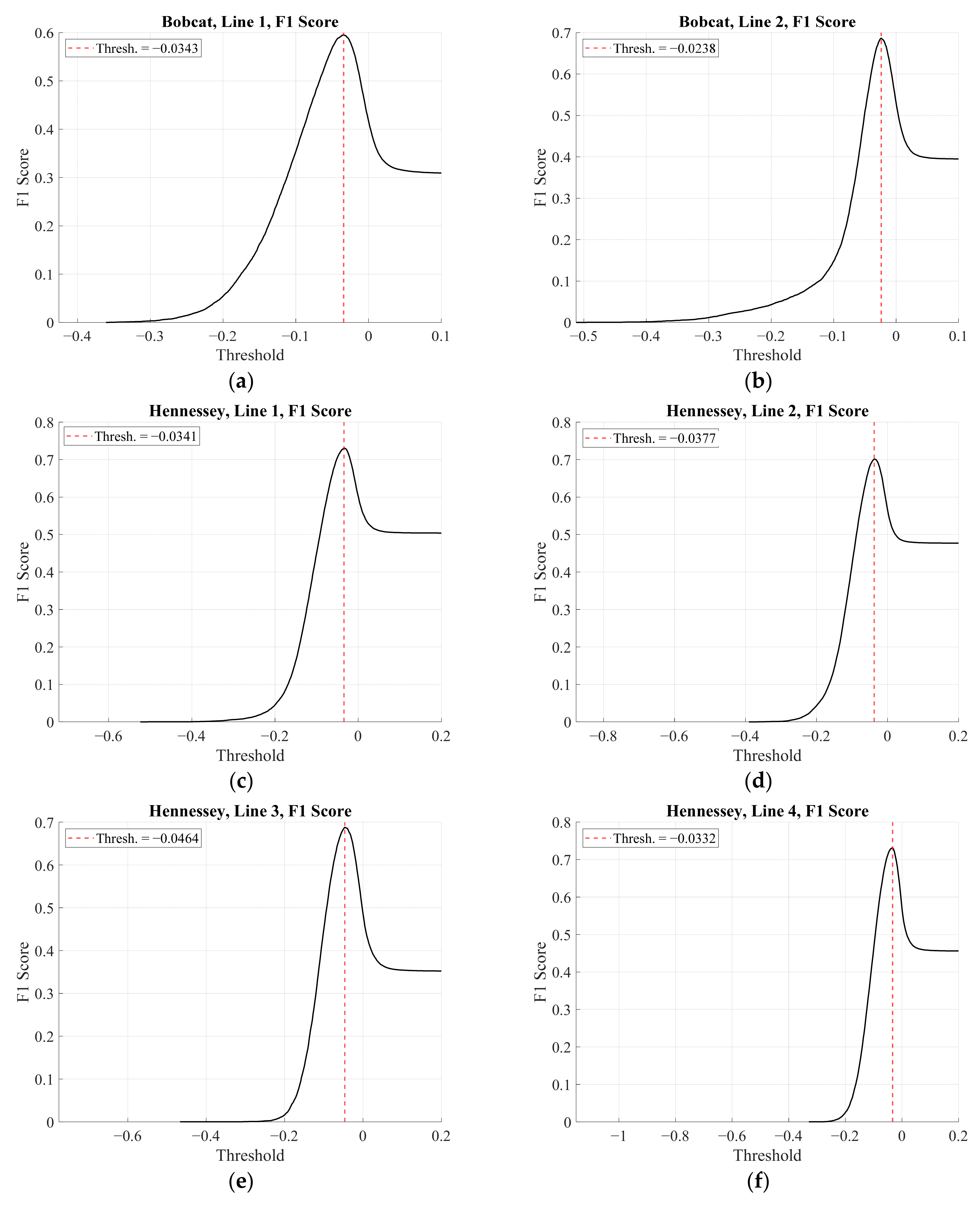
4.2. ROC Curves and F1 Score Results

Using the RVI change results together with the fire GIS perimeters and the Landsat 8-based dNBR, a ROC curve was calculated for each repeat-track line for each wildfire analyzed. The analysis was repeated with NRCS values multi-looked to spatial resolutions of ~ 5 (inherent SAR resolution), 25, 50, 100, 200, and 500 m by recomputing the RVI at each resolution. A corresponding “truth” reference map marking “burned” and “not burned” pixels was also developed for each resolution using the mode of the finest resolution ground truth pixels within a coarser map cell. A threshold detector was applied to the RVI change at each spatial resolution, with any RVI change less than the threshold receiving a ‘burned’ classification and ‘not burned’ otherwise. Missed detections and false alarms were then identified by comparing the two maps. Because the Caldor fire dataset has only 5 days between UAVSAR flights, Landsat 8 coverage was not available for use in establishing the reference map. Caldor measurements are therefore excluded from the ROC and F1 studies. The Landsat 8-based dNBR images used in ground truthing for the Bobcat and Hennesey fire are shown in Figure 6, with ground truth reference maps at 100 m spatial resolution provided in Figure 7. It is noted here that the thresholds used to classify burn severity are based on the Landsat8 dNBR thresholds commonly used (regrowth < −0.1; unburned: −0.1–+0.1; low severity: +0.1–+0.27; moderate severity: +0.27–+0.66; high severity: >+0.66) [91].

ROC curves at varying spatial resolutions for both the Bobcat and Hennessy fires are presented in Figure 8 and compared to a 1:1 line indicating a “random guess” detector. For all UAVSAR repeat-tracks across both fires, the results show a detection performance that improves as the spatial resolution is degraded (i.e., less speckle influence and more accurate RVI measurement) and that is slightly better for Bobcat line 2 compared to Bobcat line 1 and the Hennessey fire. The tradeoffs of the detection and false alarm probabilities are also evident.

The F1 score was also calculated as a function of the detector threshold for all repeat-track lines for the Bobcat and Hennessey fires. The results at 100 m spatial resolution are shown in Figure 9 along with a vertical red line indicating the maximum F1 score for each individual case, with the resulting threshold value labeled in the legend. A full statistical analysis for each maximum F1 score for varying spatial resolutions is presented in

Table 3. Table of F1 score results for UAVSAR detection of Bobcat and Hennessey fires.

Resolution:	Threshold:	F1 Score:	Pd:	Pfa:
Bobcat, Line 1
5 m	−0.0657	0.3933	43.81%	17.16%
25 m	−0.0582	0.4351	45.13%	13.72%
50 m	−0.0466	0.5007	49.61%	10.66%
100 m	−0.0343	0.5953	57.33%	7.86%
200 m	−0.0248	0.6831	67.26%	6.71%
500 m	−0.0166	0.7399	78.08%	7.44%
Bobcat, Line 2
5 m	−0.0264	0.4437	55.89%	30.51%
25 m	−0.0274	0.4841	56.67%	24.58%
50 m	−0.0280	0.5627	58.90%	16.13%
100 m	−0.0238	0.6865	67.89%	9.71%
200 m	−0.0176	0.7973	81.67%	7.79%
500 m	−0.0151	0.8923	91.86%	4.86%
Hennessey, Line 1
5 m	−0.0370	0.5735	63.55%	28.78%
25 m	−0.0422	0.6159	63.22%	20.96%
50 m	−0.0390	0.6694	66.85%	16.45%
100 m	−0.0341	0.7305	71.29%	12.13%
200 m	−0.0294	0.7721	76.17%	10.90%
500 m	−0.0252	0.7984	82.51%	12.52%
Hennessey, Line 2
5 m	−0.0361	0.53689	61.58%	22.38%
25 m	−0.0406	0.5775	61.28%	23.25%
50 m	−0.0412	0.6312	62.75%	16.43%
100 m	−0.0377	0.7010	66.46%	10.56%
200 m	−0.0294	0.7558	73.40%	9.55%
500 m	−0.0279	0.7912	77.24%	8.09%
Hennessey, Line 3
5 m	−0.0512	0.4755	56.28%	22.38%
25 m	−0.0532	0.5240	56.57%	16.49%
50 m	−0.0491	0.5952	61.02%	12.12%
100 m	−0.0464	0.6879	65.60%	6.82%
200 m	−0.0384	0.7636	74.22%	5.38%
500 m	−0.0347	0.8080	79.05%	4.31%
Hennessey, Line 4
5 m	−0.0389	0.5693	62.08%	23.97%
25 m	−0.403	0.6092	63.16%	18.97%
50 m	−0.0419	0.6652	64.75%	12.71%
100 m	−0.0332	0.7309	71.98%	10.47%
200 m	−0.0237	0.7792	74.13%	6.72%
500 m	−0.0307	0.81656	78.11%	5.47%

and includes the associated probability of detection and the probability of false alarm for each UAVSAR line investigated.

The results again highlight an increasing trend in performance as the spatial resolution becomes coarser, as seen in the ROC curves (increased probability of detection vs. decreased probability of false alarm). Overall, the methods at 500 m resolution result in a probability of detection of 77.24% or greater and a probability of false alarm of 12.52% or less. At the finest ~5 m resolution, the probability of detection is 43.81% or greater and the probability of false alarm is 30.51% or less. At 100 m resolution, the results show a probability of detection of 57.33% or greater and a probability of false alarm of 12.13% or less. The highest probability of detection at 100 m is 71.98% for the southern-most UAVSAR line over the Hennessey fire, and the smallest probability of false alarm is 6.82% for Hennessey line 3. In general, the results for the Hennessey fire at 100 m show higher probabilities of detection, while the Bobcat fire shows smaller probabilities of false alarm. These results highlight the tradeoff of detector performance versus spatial resolution, with an “optimal” value in this tradeoff depending on the application of interest. Finer resolutions may be warranted for monitoring variations in a fire at the regional level, while coarser resolutions may be warranted for identifying new fire locations on a global scale.

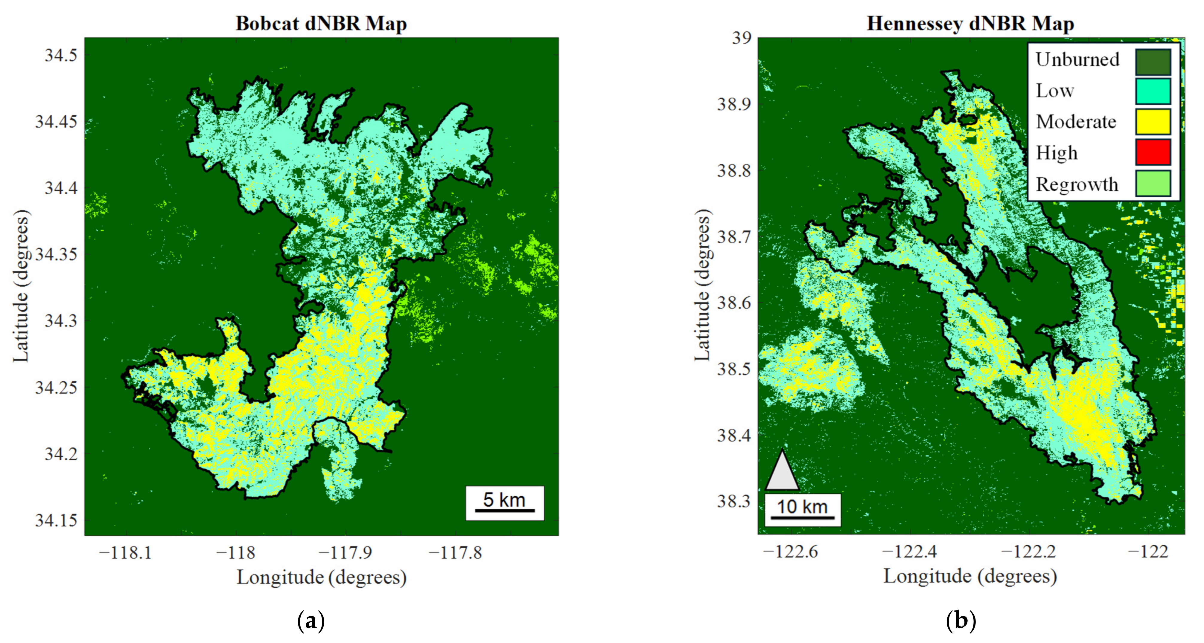
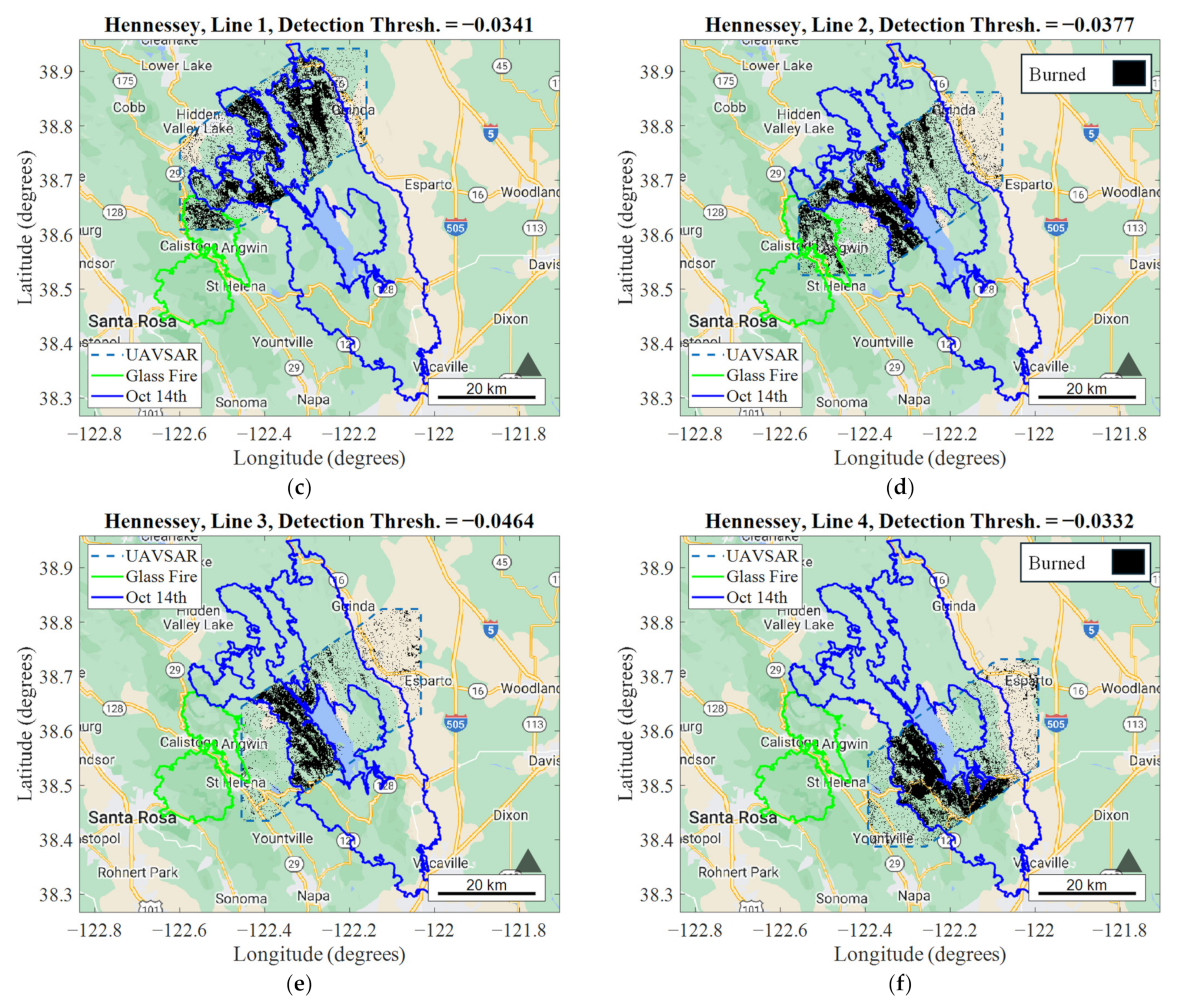
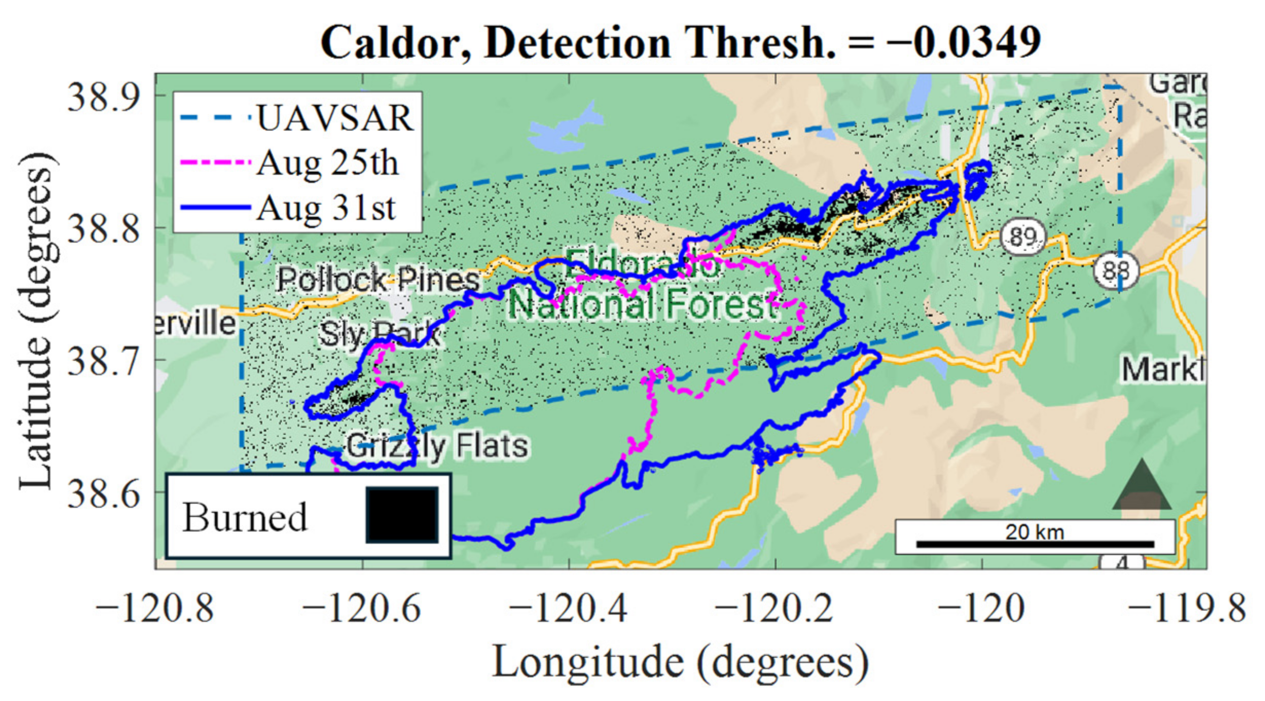
4.3. Threshold Detection Results

Using the threshold values that maximized the 100 m F1 score for each flight track (Table 3), a wildfire detection map can be created for each repeat-track line. The resulting fire detection maps (burned areas marked with black pixels) are presented at 100 m resolution in Figure 10. The results again show a high degree of correlation, as indicated by the MCC, between the detected “burned” pixels and the reference maps (Figure 7) for each fire. Spatial correlations (MCC values) between Figure 7 and Figure 10 are presented in

Table 4. Matthews correlation coefficients for detection results at varying spatial resolutions.

Site:	5m:	25 m:	50 m:	100 m:	200 m:	500 m:
Bobcat Line 1	0.2467	0.3055	0.3924	0.5099	0.6129	0.6788
Bobcat Line 2	0.2254	0.2934	0.4153	0.5863	0.7274	0.8542
Hennessey Line 1	0.3336	0.4173	0.5043	0.5991	0.6571	0.6896
Hennessey Line 2	0.2901	0.3694	0.4647	0.5770	0.6492	0.7011
Hennessey Line 3	0.3060	0.3808	0.4805	0.6094	0.7034	0.7599
Hennessey Line 4	0.3651	0.4334	0.5289	0.6207	0.6955	0.7469

. Additionally, all detection images presented show false detections that take on a generally granular pattern outside of the fire perimeters that is typical of the inherent speckle noise present in SAR imagery [92,93]. While detection imagery for other spatial resolutions is not presented in this study to limit the number of figures and focus on potential NISAR-like applications, the results generally highlight an increase in these speckle-like false detections at much finer resolutions that decrease as the spatial resolution becomes coarser. Although advanced speckle filtering (i.e., Lee or Wiener filtering) of the raw UAVSAR measurements was not applied, the trend nevertheless highlights that the simple averaging method used to multi-look to coarser spatial resolutions performs de facto filtering that decreases speckle influences. While speckle noise is common in SAR imagery, larger “clumps” of false detections may suggest other influences that are discussed in the next section.

For both Bobcat line 1 and line 2, the majority of burned pixels and the largest concentrations lie within the burn perimeters of the two dates, again highlighting the ability to identify new burning. Both lines also identify pixels within the initial Sept 18th “continued burning” perimeter, as discussed previously, although this is more prevalent in line 2 than line 1 for reasons that are under continued investigation. The spatial correlations (MCC) between the RVI classifications and the corresponding truth maps at 100 m spatial resolution are 0.5099 and 0.5863 for lines 1 and 2, respectively. Burning occurring in the Ranch2 fire is also identified. The detection results agree with other wildfire metrics such as MTBS burn severity maps [83,84], LANDFIRE 2020 vegetation disturbance burn classification [85], and MASTER fire intensity/burn severity data [86]. Furthermore, the detection results show an improvement in detections over the HV-only approach used in [48]. However, it should be noted that [48] uses different UAVSAR dates (pre-fire and post-fire) to map burn scarring in their analysis, rather than the active burning over a shorter period of time that this study examines. It should also be noted that the Bobcat region was undergoing long-term drought conditions at the time of burning [11,48,94,95], and this may have led to vegetation losses or decreases in vegetation health that led to false alarms. Finally, a cluster of false alarms in the northeast region of line 1 appears to coincide with an urbanized/residential area that is not flagged. Due to the time of year and the vicinity of the fire, it is possible that these false alarms are triggered by a seasonal loss of vegetation in this residential region or possible mitigation efforts to prevent further burning or damage to this area.

The Hennessey results (Figure 10c–f) again show the highest fraction of burned pixels within the perimeters of the Hennessey and nearby Glass fires. The areas of burned pixels detected correlate well with the reference maps in Figure 7, as indicated by the MCC, for all four lines (see Table 4, MCC results). The Hennessey fire provides an example of utilizing this method to estimate continued burn extent activity within a contained event. Spatial correlations (indicated by MCC) of 0.5991, 0.5770, 0.6094, and 0.6207 are obtained between the RVI estimated and truth burned area maps at 100 m spatial resolution. The detection results for the Hennessey fire also show agreement with other fire activity metrics such as MTBS severity [83,84], LANDFIRE 2020 vegetation disturbance [85], and soil burn severity, as highlighted in the post-fire analysis [88]. It should again be noted that while the Hennessey region typically receives more rainfall than Bobcat region, there were still ongoing drought conditions in California at the time that may have influenced false alarms [95,96,97].

The MCC information summarized in Table 4 shows an increase in correlation as the spatial resolution is degraded, consistent with the improvements in detection performance as the resolution is coarsened. Line 2 for the Bobcat fire and Hennessey lines 3 and 4 show a 500 m correlation of 0.7469 or higher, while Hennesey lines 1 and 4 show the highest correlations (maximum 0.36) at 5 m resolution.

The detections and spatial correlation information reported in the preceding discussions used a threshold for each line that maximized the F1 score of that line when compared to the corresponding reference information. While the thresholds used were similar (ranging from −0.0238 to −0.0464, see titles of Figure 10a–f), it is desirable, if possible, to identify a single threshold value that could be used in all cases while retaining reasonable performance. A single combined threshold value using data from all six repeat-track lines of the combined Hennessey and Bobcat fires was therefore determined using the simple average of all thresholds determined for each spatial resolution. The resulting threshold values determined in this manner are listed as a function of spatial resolution in

Table 5. Table of universal thresholds for testing Caldor Fire.

Resolution	Threshold
5 m	−0.0425
25 m	−0.0436
50 m	−0.0410
100 m	−0.0349
200 m	−0.0287
500 m	−0.0250

.

The derived 100 m threshold (−0.0349) was then applied to the Caldor fire for which only reported fire perimeters and no usable coincident LandSat data were available. The resulting detection map is presented in Figure 11 and shows the concentration of detected locations in the region between the two flight date perimeters, but there are fewer detections within the earlier perimeter. This concentration is reasonable given the 5-day difference between flights in this case; so, vegetation changes in already burned areas may be moderate when compared to newly burned areas. The results generally show a high degree of correlation with known progression maps. Furthermore, a study by the U.S. Department of Agriculture Forest Service [90] assessed a post-fire framework at the Caldor site that provides in-depth analyses on vegetation-based damages using products such as Rapid Assessment on Vegetation Condition (RAVG), Basal Area Percent Cover, Basal Area Loss, and Departure from Natural Range of Variability (NRV). The report found high degrees of vegetation loss/damage in the areas identified as “burned” in Caldor, shown in Figure 11. Finally, the burned area detections in Figure 11 show agreement with known burned areas from other metrics such as MTBS burn severity [84] and LANDFIRE 2021 vegetation disturbance [89]. Overall, the results for the Caldor fire highlight the potential for the development of a universal or regional threshold value of changes in the RVI to monitor wildfire progression.

4.4. RVI Measurement Errors

Both speckle and thermal noise can cause errors in attempts to determine the RVI. Thermal noise effects are related to the noise Equivalent Sigma Zero (NESZ) or noise floor of the measurement, which represents the NRCS level of the inherent noise in the absence of a transmitted signal (i.e., independent additive noise) [98]. Speckle noise effects arise due to the inherently random nature of scattering from Earth’s surface. Both thermal and speckle noise effects are reduced by the “multi-looking” (i.e., averaging) of SAR measurements, as described by the system’s K_p parameter. Other system calibration errors can also contribute to errors in the measurement of the RVI. While further quantitative studies of these aspects are currently in process and are not reported here, in general, the very low NESZ and significant multi-looking of the UAVSAR [99,100] dataset enable RVI measurements of sufficient quality to distinguish burned and non-burned regions.

5. Conclusions

A method for monitoring wildfire activity using changes in the RVI was presented. The results demonstrate that the RVI-based threshold wildfire detector showed high spatial correlation with known wildfire burn extent perimeters and other fire activity indicators, such as Landsat 8-based dNBR. The method proved effective across multiple fires covering different environmental regimes and at varied spatial resolutions, indicating an approach with significant potential for broader application in wildfire monitoring.

Future research could explore the integration of this method with other remote sensing techniques to improve the accuracy and real-time application. Additionally, extending this study to include a wider range of wildfire events and different geographic regions would help to further validate and refine the approach. This could mean adding more wildfires from 2022 and 2023 with UAVSAR coverage, as well as fine-tuning an application for the upcoming NISAR mission.

The ability to accurately detect and monitor wildfires using SAR-based methods has significant practical implications for fire management and mitigation efforts. By providing timely and reliable data on fire progression and locations, this method can aid in the allocation of resources, the planning of evacuation routes, and the overall strategy for combating wildfires. The implementation of this technique in both current and future operational systems could enhance the effectiveness of wildfire response and management, thereby further minimizing fire-related damage and costs.

While the RVI change detection method has shown promising results, some limitations still need to be addressed. The impact of measurement errors requires further analysis given the relatively small changes in the RVI that were used in the detection process. For implementation on global or regional scales, future research should emphasize developing thresholds based on characteristics such as region, season, climate, and/or vegetation type.

In conclusion, the RVI change detection threshold method offers an apparently robust and reliable methodology for monitoring wildfire progression using polarimetric SAR measurements. The success of this method in identifying burned areas and correlating these with other fire indicators and products suggests its potential for operational use in wildfire management and implementation in future SAR missions, such as the upcoming NISAR mission. Continued research and development in this area will be crucial in enhancing our capabilities to monitor and respond to wildfire events effectively.

References

1. Pausas, J.G.; Keeley, J.E. Wildfires as an ecosystem service. Front. Ecol. Environ. 2019, 17, 289–295. [Google Scholar] [CrossRef]
2. Hutto, R.L. The Ecological Importance of Sever Wildfires: Some Like It Hot. Ecol. Appl. 2008, 18, 1827–1834. [Google Scholar] [CrossRef]
3. Keane, R.E.; Agee, J.K.; Fule, P.; Keeley, J.E.; Key, C.; Kitchen, S.G.; Miller, R.; Schulte, L.A. Ecological effects of large fires on US Landscapes: Benefit or catastrophe? Int. J. Wildland Fire 2008, 17, 696–712. [Google Scholar] [CrossRef]
4. Keane, R.E.; Karau, E. Evaluating the ecological benefits of wildfire by integrating fire and ecosystem simulation models. Ecol. Model. 2010, 221, 1162–1172. [Google Scholar] [CrossRef]
5. Leblon, B.; Bourgeau-Chavez, L.; San-Miguel-Ayanz, J. Use of remote sensing in wildfire management. In Sustainable Development—Authoritative and Leading Edge Content for Environmental Management; IntechOpen: London, UK, 2012; pp. 55–82. [Google Scholar]
6. Stavi, I. Wildfires in grasslands and shrublands: A review of impacts on vegetation, soil, hydrology, and geomorphology. Water 2019, 11, 1042. [Google Scholar] [CrossRef]
7. Williams, A.P.; Abatzoglou, J.T.; Gershunov, A.; Guzman-Morales, J.; Bishop, D.A.; Balch, J.K.; Lettenmaier, D.P. Observed impacts of anthropogenic climate change on wildfire in California. Earth’s Future 2019, 7, 892–910. [Google Scholar] [CrossRef]
8. Sharma, S.; Dhakal, K. Boots on the ground and eyes in the sky: A perspective on estimating fire danger from soil moisture content. Fire 2021, 4, 45. [Google Scholar] [CrossRef]
9. Dennison, P.E.; Brewer, S.C.; Arnold, J.D.; Moritz, M.A. Large wildfire trends in the Western United States, 1984–2011. Geophys. Res. Lett. 2014, 41, 2928–2933. [Google Scholar] [CrossRef]
10. National Interagency Coordination Center, Geographic Area Coordination Center. 2020 National Large Incident Year-to-Date Report. 2020. Available online: https://gacc.nifc.gov/sacc/predictive/intelligence/NationalLargeIncidentYTDReport.pdf (accessed on 20 January 2023).
11. National Interagency Coordination Center. Wildland Fire Summary and Statistics Annual Report. 2020. Available online: https://www.nifc.gov/sites/default/files/NICC/2-Predictive%20Services/Intelligence/Annual%20Reports/2020/annual_report_0.pdf (accessed on 20 January 2023).
12. California Department of Forestry and Fire Protection (CAL FIRE). 2020 Wildfire Activity Statistics (CALFIRE Redbook). 2020. Available online: https://34c031f8-c9fd-4018-8c5a-4159cdff6b0d-cdn-endpoint.azureedge.net/-/media/calfire-website/our-impact/fire-statistics/2020-wildfire-activity-stats.pdf?rev=da776d6b864342edb2fe0782b1afd9af&hash=17B19313E6A54CBE1D4693FAAC27F23C/ (accessed on 20 January 2023).
13. Pereira, P.; Francos, M.; Brevik, E.C.; Ubeda, X.; Bogunovic, I. Post-fire Soil Management. Curr. Opin. Environ. Sci. Health 2018, 5, 26–32. [Google Scholar] [CrossRef]
14. Kalabokidis, K.D. Effects of Wildfire Suppression Chemicals on People and the Environment—A Review. Glob. Nest Int. J. 2000, 2, 129–137. [Google Scholar]
15. National Park Service. Fire Monitoring Handbook. Available online: https://www.nps.gov/orgs/1965/upload/fire-effects-monitoring-handbook.pdf (accessed on 1 December 2023).
16. Allison, R.; Johnston, J.; Craig, G.; Jennings, S. Airborne Optical and Thermal Remote Sensing for Wildfire Detection and Monitoring. Sensors 2016, 16, 1310. [Google Scholar] [CrossRef]
17. Nolde, M.; Plank, S.; Riedlinger, T. Utilization of Hyperspectral Remote Sensing Imagery for Improving Burnt Area Mapping Accuracy. Remote Sens. 2021, 13, 5029. [Google Scholar] [CrossRef]
18. Hua, L.; Shao, G. The Progress of Operational Forest Fire Monitoring with Infrared Remote Sensing. J. For. Res. 2016, 28, 215–229. [Google Scholar] [CrossRef]
19. Adam, E.; Mutanga, O.; Rugege, D. Multispectral and Hyperspectral Remote Sensing for Identification and Mapping of Wetland Vegetation: A Review. Wetl. Ecol. Manag. 2009, 18, 281–296. [Google Scholar] [CrossRef]
20. Hislop, S.; Jones, S.; Soto-Berelov, M.; Skidmore, A.; Haywood, A.; Nguyen, T.H. Using Landsat Spectral Indices in Time-Series to Assess Wildfire Disturbance and Recovery. Remote Sens. 2018, 10, 460. [Google Scholar] [CrossRef]
21. João, T.; João, G.; Bruno, M.; João, H. Indicator-Based Assessment of Post-Fire Recovery Dynamics Using Satellite NDVI Time-Series. Ecol. Indic. 2018, 89, 199–212. [Google Scholar] [CrossRef]
22. Ulaby, F.T.; Long, D.G.; Blackwell, W.; Elachi, C.; Fung, A.; Ruf, C.; Sarabandi, K.; van Zyl, J.; Zebker, H. Microwave Radar and Radiometric Remote Sensing; The University of Michigan Press: Ann Arbor, MI, USA, 2017. [Google Scholar]
23. European Space Agency (ESA). Copernicus Sentinel Data. 2021. Available online: https://browser.dataspace.copernicus.eu/ (accessed on 1 August 2023).
24. Spoto, F.; Sy, O.; Laberinti, P.; Martimort, P.; Fernandez, V.; Colin, O.; Hoersch, B.; Meygret, A. Overview of Sentinel-2. In Proceedings of the 2012 IEEE International Geoscience and Remote Sensing Symposium, Munich, Germany, 22–27 July 2012; pp. 1707–1710. [Google Scholar]
25. Vermote, E. NOAA CDR Program, (2019): NOAA Climate Data Record (CDR) of AVHRR Normalized Difference Vegetation Index, Version 5, [2018–2022], NOAA National Centers for Environmental Information. Available online: https://www.ncei.noaa.gov/data/land-normalized-difference-vegetation-index/access/ (accessed on 1 August 2023).
26. Moravec, D.; Komárek, J.; López-Cuervo Medina, S.; Molina, I. Effect of Atmospheric Corrections on NDVI: Intercomparability of Landsat 8, Sentinel-2, and UAV Sensors. Remote Sens. 2021, 13, 3550. [Google Scholar] [CrossRef]
27. Tsai, Y.-L.S.; Dietz, A.; Oppelt, N.; Kuenzer, C. Remote Sensing of Snow Cover Using Spaceborne SAR: A Review. Remote Sens. 2019, 11, 1456. [Google Scholar] [CrossRef]
28. United States Department of Agriculture, Forest Service. 2019 Forest Service-NASA Joint Applications Workshop: Satellite Data to Support Natural Resource Management: A Framework for Aligning NASA Products with Land Management Agency Needs. 2023. Available online: https://www.fs.usda.gov/rm/pubs_series/rmrs/gtr/rmrs_gtr436.pdf (accessed on 1 June 2024).
29. Forgotson, C.; O’Neill, P.E.; Carrera, M.L.; Belair, S.; Das, N.N.; Mladenova, I.E.; Bolten, J.D.; Jacobs, J.M.; Cho, E.; Escobar, V.M. How Satellite Soil Moisture Data Can Help to Monitor the Impacts of Climate Change: SMAP Case Studies. IEEE J. Sel. Top. Appl. Earth Obs. Remote Sens. 2020, 13, 1590–1596. [Google Scholar] [CrossRef]
30. Bernardino, P.N.; Oliveira, R.S.; Van Meerbeek, K.; Hirota, M.; Furtado, M.N.; Sanches, I.A.; Somers, B. Estimating Vegetation Water Content from Sentinel-1 C-band SAR Data Over Savanna and Grassland Ecosystems. Environ. Res. Lett. 2024, 19, 034019. [Google Scholar] [CrossRef]
31. Patil, A.; Singh, G.; Rüdiger, C. Retrieval of Snow Depth and Snow Water Equivalent Using Dual Polarization SAR Data. Remote Sens. 2020, 12, 1183. [Google Scholar] [CrossRef]
32. Carstairs, H.; Mitchard, E.T.A.; McNicol, I.; Aquino, C.; Burt, A.; Ebanega, M.O.; Dikongo, A.M.; Bueso-Bello, J.-L.; Disney, M. An Effective Method for InSAR Mapping of Tropical Forest Degradation in Hilly Areas. Remote Sens. 2022, 14, 452. [Google Scholar] [CrossRef]
33. Wanders, N.; Karssenberg, D.; de Roo, A.; de Jong, S.M.; Bierkens, M.F. The Suitability of Remotely Sensed Soil Moisture for Improving Operational Flood Forecasting. Hydrol. Earth Syst. Sci. 2014, 18, 2343–2357. [Google Scholar] [CrossRef]
34. Horton, D.; Johnson, J.T.; Al-Khaldi, M.; Baris, I.; Park, J.; Bindlish, R. Soil Moisture During 2015 Spring Flood Events from the SMAP Radar Time-Series Ratio Algorithm. In Proceedings of the 2024 United States National Committee of URSI National Radio Science Meeting (USNC-URSI NRSM), Boulder, CO, USA, 9–12 January 2024; p. 352. [Google Scholar]
35. Eswar, R.; Das, N.N.; Poulsen, C.; Behrangi, A.; Swigart, J.; Svoboda, M.; Entekhabi, D.; Yueh, S.; Doorn, B.; Entin, J. SMAP Soil Moisture Change as an Indicator of Drought Conditions. Remote Sens. 2018, 10, 788. [Google Scholar] [CrossRef]
36. Olen, S.; Bookhagen, B. Mapping Damage-Affected Areas after Natural Hazard Events Using Sentinel-1 Coherence Time Series. Remote Sens. 2018, 10, 1272. [Google Scholar] [CrossRef]
37. Ottmar, R.D. Wildland Fire Emissions, Carbon, and Climate: Modeling Fuel Consumption. For. Ecol. Manag. 2014, 317, 41–50. [Google Scholar] [CrossRef]
38. Chen, H.; White, J.C.; Beaudoin, A. Derivation and Assessment of Forest-Relevant Polarimetric Indices Using RCM Compact-Pol Data. Int. J. Remote Sens. 2023, 44, 381–406. [Google Scholar] [CrossRef]
39. Kim, Y.; van Zyl, J.J. A Time-series Approach to Estimate Soil Moisture Using Polarimetric Radar Data. IEEE Trans. Geosci. Remote Sens. 2009, 47, 2519–2527. [Google Scholar]
40. Saatchi, S. SAR Methods for Mapping and Monitoring Forest Biomass. In The SAR Handbook: Comprehensive Methodologies for Forest Monitoring and Biomass Estimation, 1st ed.; Flores-Anderson, A.I., Herndon, K.E., Thapa, R.B., Cherrington, E., Eds.; SilvaCarbon Program: Washington, DC, USA, 2019; pp. 207–246. [Google Scholar]
41. Huang, Y.; Walker, J.P.; Gao, Y.; Wu, X.; Monerris, A. Estimation of Vegetation Water Content from the Radar Vegetation Index at L-band. IEEE Trans. Geosci. Remote Sens. 2016, 54, 981–989. [Google Scholar] [CrossRef]
42. Kim, Y.; Jackson, T.; Bindlish, R.; Lee, H.; Hong, S. Radar Vegetation Index for Estimating the Vegetation Water Content of Rice and Soybean. IEEE Geosci. Remote Sens. Lett. 2012, 9, 564–568. [Google Scholar]
43. Chang, J.G.; Shoshany, M.; Oh, Y. Polarimetric Radar Vegetation Index for Biomass Estimation in Desert Fringe Ecosystems. IEEE Trans. Geosci. Remote Sens. 2018, 56, 7102–7108. [Google Scholar] [CrossRef]
44. Szigarski, C.; Jagdhuber, T.; Baur, M.; Thiel, C.; Parrens, M.; Wigneron, J.-P.; Piles, M.; Entekhabi, D. Analysis of the Radar Vegetation Index and Potential Improvements. Remote Sens. 2018, 10, 1776. [Google Scholar] [CrossRef]
45. Haldar, D.; Verma, A.; Kumar, S.; Chauhan, P. Estimation of Mustard and Wheat Phenology Using Multi-date Shannon Entropy and Radar Vegetation Index from Polarimetric Sentinel-1. Geocarto Int. 2021, 37, 5935–5962. [Google Scholar] [CrossRef]
46. Thompson, A.A. Overview of the RADARSAT Constellation Mission. Can. J. Remote Sens. 2015, 41, 401–407. [Google Scholar] [CrossRef]
47. NASA/ISRO Synthetic Aperture Radar Mission. NISAR Handbook. Available online: https://nisar.jpl.nasa.gov/system/documents/files/26_NISAR_FINAL_9-6-19.pdf (accessed on 1 May 2024).
48. An, K.; Jones, C.; Lou, Y. Developing a Detection and Monitoring Framework for Wildfire Regimes with L-Band Polarimetric SAR. Submitted to AGU Earth and Space Science. 2023. Available online: https://essopenarchive.org/users/600587/articles/632138-developing-a-detection-and-monitoring-framework-for-wildfire-regimes-with-l-band-polarimetric-sar (accessed on 1 June 2024).
49. Mandai, D.; Bhogapurapu, N.R.; Kumar, V.; Dey, S.; Ratha, D.; Bhattacharya, A.; Loper-Sanchez, J.M.; McNairn, H.; Rao, Y.S. Vegetation Monitoring Using a New Dual-POL Radar Vegetation Index: A Preliminary Study with Simulated NASA-ISRO SAR (NISAR) L-band Data. In Proceedings of the IGARSS 2020—2020 IEEE International Geoscience and Remote Sensing Symposium, Waikoloa, HI, USA, 26 September–2 October2020; pp. 4870–4873. [Google Scholar]
50. NASA/JPL-Caltech. UAVSAR Data. Available online: https://uavsar.jpl.nasa.gov/cgi-bin/data.pl (accessed on 15 August 2023).
51. Peterson, W.W.; Birdsall, T.G. The Theory of Signal Detectability. Trans. IRE Prof. Group Inf. Theory 1953, 4, 171–212. [Google Scholar] [CrossRef]
52. Candy, J.; Breitfeller, E. Receiver Operating Characteristic (ROC) Curves: An Analysis Tool for Detection Performance. In No. LLNL-TR-642693; Lawrence Livermore National Lab: Livermore, CA, USA, 2013. [Google Scholar]
53. Goutte, C.; Gaussier, E. A Probabilistic Interpretation of Precision, Recall and F-score, with Implication for Evaluation. In Proceedings of the European Conference on Information Retrieval, Berlin/Heidelberg, Germany, 21–23 March 2005; pp. 345–359. [Google Scholar]
54. Bechtel, T.; Capineri, L.; Windsor, C.; Inagaki, M.; Ivashov, S. Comparison of ROC Curves for Landmine Detection by Holographic Radar with ROC Data from Other Methods. In Proceedings of the 2015 8th International Workshop on Advanced Ground Penetrating Radar (IWAGPR), Florence, Italy, 7–10 July 2015; pp. 1–4. [Google Scholar]
55. Chang, C.-I. An Effective Evaluation Tool for Hyperspectral Target Detection: 3D Receiver Operating Characteristic Curve Analysis. IEEE Trans. Geosci. Remote Sens. 2021, 59, 5131–5153. [Google Scholar] [CrossRef]
56. Zhang, L.; Gao, G.; Chen, C.; Gao, S.; Yao, L. Compact Polarimetric Synthetic Aperture Radar for Target Detection: A Review. IEEE Geosci. Remote Sens. Mag. 2022, 10, 115–152. [Google Scholar] [CrossRef]
57. Waldeland, A.; Reksten, J.; Salberg, A.-B. Avalanche Detection in SAR Images Using Deep Learning. In Proceedings of the IGARSS 2018—2018 IEEE International Geoscience and Remote Sensing Symposium, Valencia, Spain, 22–27 July 2018; pp. 2386–2389. [Google Scholar]
58. Rapuzzi, A.; Nattero, C.; Pelich, R.; Chini, M.; Campanella, P. CNN-based Building Footprint Detection from Sentinel-1 SAR Imagery. In Proceedings of the IGARSS 2020—2020 IEEE International Geoscience and Remote Sensing Symposium, Waikoloa, HI, USA, 26 September–2 October 2020; pp. 1707–1710. [Google Scholar]
59. Ng, W.; Wang, G.; Siddhartha; Lin, Z.; Dutta, B.J. Range-Doppler Detection in Automotive Radar with Deep Learning. In Proceedings of the 2020 International Joint Conference on Neural Networks (IJCNN), Glasgow, UK, 19–24 July 2020; pp. 1–8. [Google Scholar]
60. Palffy, A.; Dong, J.; Kooij, J.F.; Gavrila, D.M. CNN-Based Road User Detection Using the 3D Radar Cube. IEEE Robot. Autom. Lett. 2020, 5, 1263–1270. [Google Scholar] [CrossRef]
61. California Department of Forestry and Fire Protection (CAL FIRE). Fire Perimeters Through. 2021. Available online: https://frap.fire.ca.gov/mapping/gis-data/ (accessed on 20 January 2023).
62. Keeley, J.E. Fire Intensity, Fire Severity and Burn Severity: A Brief Review and Suggested Usage. Int. J. Wildland Fire 2009, 18, 116–126. [Google Scholar] [CrossRef]
63. Roy, D.P.; Boschetti, L.; Trigg, S.N. Remote Sensing of Fire Severity: Assessing the Performance of the Normalized Burn Ratio. IEEE Geosci. Remote Sens. Lett. 2006, 3, 112–116. [Google Scholar] [CrossRef]
64. Escuin, S.; Navarro, R.; Fernández, P. Fire Severity Assessment by Using NBR (Normalized Burn Ratio) and NDVI (Normalized Difference Vegetation Index) Derived from Landsat TM/ETM Images. Int. J. Remote Sens. 2007, 29, 1053–1073. [Google Scholar] [CrossRef]
65. Cardil, A.; Mola-Yudego, B.; Blázquez-Casado, Á.; González-Olabarria, J.R. Fire and Burn Severity Assessment: Calibration of Relative Differenced Normalized Burn Ratio (RdNBR) with Field Data. J. Environ. Manag. 2019, 235, 342–349. [Google Scholar] [CrossRef]
66. Loveland, T.R.; Irons, J.R. Landsat 8: The Plans, the Reality, and the Legacy. Remote Sens. Environ. 2016, 185, 1–6. [Google Scholar] [CrossRef]
67. Landsat 8 Data Available from the U.S. Geological Survey. Available online: https://earthexplorer.usgs.gov/ (accessed on 10 December 2023).
68. Liu, L. Encyclopedia of Database Systems; Springer: New York, NY, USA, 2009. [Google Scholar]
69. Stoica, P.; Babu, P. Pearson–Matthews Correlation Coefficients for Binary and Multinary Classification. Signal Process 2024, 222, 109511. [Google Scholar] [CrossRef]
70. Chicco, D.; Jurman, G. The Advantages of the Matthews Correlation Coefficient (MCC) over F1 Score and Accuracy in Binary Classification Evaluation. BMC Genom. 2020, 21, 6. [Google Scholar] [CrossRef] [PubMed]
71. Chicco, D.; Warrens, M.J.; Jurman, G. The Matthews Correlation Coefficient (MCC) is More Informative than Cohen’s Kappa and Brier Score in Binary Classification Assessment. IEEE Access 2021, 9, 78368–78381. [Google Scholar] [CrossRef]
72. Hensley, S.; Wheeler, K.; Sadowy, G.; Jones, C.; Shaffer, S.; Zebker, H.; Miller, T.; Heavey, B.; Chuang, E.; Chao, R.; et al. The UAVSAR Instrument: Description and First Results. In Proceedings of the 2008 IEEE Radar Conference, Rome, Italy, 26–30 May 2008. [Google Scholar]
73. Kauffman, E. Climate and Topography. In Atlas of the Biodiversity of California; California Department of Fish and Wildlife, Ed.; California Department of Fish and Wildlife: Sacramento, CA, USA, 2024. [Google Scholar]
74. Mooney, H.A.; Zavaleta, E. Ecosystems of California; University of California Press: Oakland, CA, USA, 2016. [Google Scholar]
75. van Wagtendonk, J.W.; Sugihara, N.G.; Stephens, S.L.; Thode, A.E.; Shaffer, K.E.; Fites-Kaufman, J.; Keeley, J.E. Fire in California’s Ecosystems, 2nd ed.; University of California Press: Oakland, CA, USA, 2018. [Google Scholar]
76. Keeley, J.E.; Syphard, A.D. Different Historical Fire–Climate Patterns in California. Int. J. Wildland Fire 2017, 26, 253–268. [Google Scholar] [CrossRef]
77. United States Forest Service. Bobcat Fire. 2020. Available online: https://www.fs.usda.gov/Internet/FSE_DOCUMENTS/fseprd868759.pdf (accessed on 1 May 2024).
78. Dewitz, J. National Land Cover Database (NLCD) 2019 Products (ver. 2.0, June 2021). U.S. Geological Survey Data. 2021. Available online: https://www.usgs.gov/centers/eros/science/national-land-cover-database (accessed on 10 January 2024).
79. California Department of Forestry and Fire Protection (CAL FIRE). LNU Lightning Complex Fire Incident Report. 2020. Available online: https://www.fire.ca.gov/incidents/2020/8/17/lnu-lightning-complex/ (accessed on 1 May 2024).
80. California Department of Forestry and Fire Protection (CAL FIRE). Caldor Fire Incident Report. 2021. Available online: https://www.fire.ca.gov/incidents/2021/8/14/caldor-fire/ (accessed on 1 August 2023).
81. National Interagency Coordination Center. Wildland Fire Summary and Statistics Annual Report. 2021. Available online: https://www.nifc.gov/sites/default/files/NICC/2-Predictive%20Services/Intelligence/Annual%20Reports/2021/annual_report_0.pdf (accessed on 20 January 2023).
82. National Aeronautics and Space Administration (NASA). NISAR Level 2 Scientific Requirements. Available online: https://nisar.jpl.nasa.gov/mission/mission-requirements/level-2-science-requirements/ (accessed on 1 May 2024).
83. Eidenshink, J.; Schwind, B.; Brewer, K.; Zhu, Z.L.; Quayle, B.; Howard, S. A Project for Monitoring Trends in Burn Severity. Fire Ecol. 2007, 3, 3–21. [Google Scholar] [CrossRef]
84. MTBS Data Access: Fire Level Burn Severity Geospatial Data (1984–2022). (2024, May—Last revised). MTBS Project (USDA Forest Service/U.S. Geological Survey). Available online: http://mtbs.gov/direct-download (accessed on 15 June 2024).
85. LANDFIRE. Disturbance Layer 2020, LANDFIRE 2.0.0; U.S. Department of the Interior, Geological Survey, and U.S. Department of Agriculture: Washington, DC, USA, 2020. Available online: http://www.landfire.gov/viewer (accessed on 15 June 2024).
86. NASA MASTER Team. Burn Severity and Fire Intensity Composites of the Bobcat Fire Captured by the MASTER Instrument on the NASA ER-2 Aircraft. ArcGIS Online. 2020. Available online: https://maps.disasters.nasa.gov/arcgis/home/item.html?id=2af9b2af0f9848f7b002fe4d47c7c927# (accessed on 15 June 2024).
87. Mukherjee, S.; Siroratttanakul, K.; Vargas-Sanabria, D. Supplementing Earth Observation with Twitter Data to Improve Disaster Assessments: A Case Study of 2020 Bobcat Fire in Southern California. In Proceedings of the 72nd International Astronautical Congress (IAC), Dubai, United Arab Emirates, 25–29 October 2021. [Google Scholar]
88. California Department of Forestry and Fire Protection (CAL FIRE)/California Department of Conservation Biological Survey. Watershed Emergency Response Team Evaluation LNU Lightning Complex Fire Hennessey Fire. 2020. Available online: https://scwa2.com/wp-content/uploads/2020/12/WERT.LNU-Lightning-Complex.Hennessey-Fire-ID-273408.pdf (accessed on 15 June 2024).
89. LANDFIRE. Disturbance Layer 2021, LANDFIRE 2.0.0; U.S. Department of the Interior, Geological Survey, and U.S. Department of Agriculture: Washington, DC, USA, 2021. Available online: http://www.landfire.gov/viewer (accessed on 15 June 2024).
90. United States Department of Agriculture Forest Service (USDA FS). Post-Fire Restoration Framework in Mixed Conifer Forests in the 2021 Caldor Fire, Eldorado National Forest and the Lake Tahoe Basin Management Unit: Restoration Opportunities in the 2021 Caldor Fire. Available online: https://www.fs.usda.gov/Internet/FSE_DOCUMENTS/fseprd1134862.pdf (accessed on 10 June 2024).
91. Wasser, L.; Cattau, M. Calculate and Plot Difference Normalized Burn Ratio (dNBR) from Landsat Remote Sensing Data in R. Earth Lab. 2020. Available online: https://www.earthdatascience.org/courses/earth-analytics/multispectral-remote-sensing-modis/calculate-dNBR-R-Landsat/ (accessed on 20 July 2024).
92. Singh, P.; Diwakar, M.; Shankar, A.; Shree, R.; Kumar, M. A Review on SAR Image and Its Despeckling. Arch. Comput. Methods Eng. 2021, 28, 4633–4653. [Google Scholar] [CrossRef]
93. Singh, P.; Shree, R. Analysis and Effects of Speckle Noise in SAR Images. In Proceedings of the 2016 2nd International Conference on Advances in Computing, Communication, & Automation (ICACCA) (Fall), Bareilly, India, 30 September–1 October 2016; pp. 1–5. [Google Scholar]
94. NASA Earth Observatory. Bobcat Fire Scorches Southern California. 2020. Available online: https://earthobservatory.nasa.gov/images/147324/bobcat-fire-scorches-southern-california (accessed on 20 July 2024).
95. NASA Science. The Climate Connections of a Record Fire Year in the US West. 2020. Available online: https://science.nasa.gov/earth/climate-change/the-climate-connections-of-a-record-fire-year-in-the-us-west/ (accessed on 20 July 2024).
96. Jones, J.; California Wildfires Triple Amid Drought after Record 2020 Fire Season. Newsweek. 2021. Available online: https://www.newsweek.com/california-wildfires-triple-amid-drought-after-record-2020-fire-season-1592706 (accessed on 20 July 2024).
97. National Drought Mitigation Center; U.S. Department of Agriculture; National Oceanic and Atmospheric Administration. United States Drought Monitor: State of California in 2020; University of Nebraska-Lincoln: Lincoln, NE, USA, 2023. [Google Scholar]
98. Yang, J.; Zhong, L.; Yuan, X.; Wang, X.; Han, B.; Hu, Y. First Assessment of Noise-Equivalent Sigma-Zero in GF3-02 TOPSAR Mode with Sea Surface Wind Speed Retrieval. Acta Oceanol. Sin. 2023, 42, 84–96. [Google Scholar] [CrossRef]
99. Fore, A.G.; Chapman, B.D.; Hawkins, B.P.; Hensley, S.; Jones, C.E.; Michel, T.R.; Muellerschoen, R.J. UAVSAR Polarimetric Calibration. IEEE Trans. Geosci. Remote Sens. 2015, 53, 3481–3491. [Google Scholar] [CrossRef]
100. Minchew, B.; Jones, C.E.; Holt, B. Polarimetric Analysis of Backscatter from the Deepwater Horizon Oil Spill Using L-band Synthetic Aperture Radar. IEEE Trans. Geosci. Remote Sens. 2012, 50, 3812–3830. [Google Scholar] [CrossRef]
Figure 1. A comparison of optical imagery taken over the Caldor wildfire on 29 August 2021, using (a) the VIIRS-based normalized difference vegetation index (NDVI) [25] and (b) Copernicus/Sentinel imagery [23]. Both images highlight the deleterious impact of fire-generated smoke on optically based observations.
Remotesensing 16 03050 g001
Figure 2. The histogram results comparing the UAVSAR-based classical RVI [50] using a pre-factor of 8 (left-hand column) and the improved RVI using a pre-factor of 6.57 (right-hand column). The comparison is performed for the 3 different regions being studied and the results are combined to highlight different dominant land classifications: (a) classical RVI; (b) improved RVI.
Remotesensing 16 03050 g002
Figure 3. A map of the wildfire test sites. The Bobcat fire of 2020 is identified by the red pentagram, the Hennessey fire of 2020 is identified by the blue pentagram, and the Caldor fire of 2021 is identified by the green pentagram.
Remotesensing 16 03050 g003
Figure 4. Wildfire site satellite imagery (left-hand column) with burn extent perimeters on UAVSAR flight dates and National Land Cover Database (NLCD) [78] maps (right-hand column) with a summary legend of the most common land class types. (a) Bobcat fire satellite image; (b) Bobcat NLCD map; (c) Hennessey fire satellite image; (d) Hennessey NLCD map; (e) Caldor fire satellite image; and (f) Caldor NLCD map.
Remotesensing 16 03050 g004aRemotesensing 16 03050 g004b
Figure 5. The change in the improved RVI, with k = 6.57, (negative values indicate RVI decrease and vegetation loss) at 100 m spatial resolution for the Bobcat wildfire using UAVSAR measurements taken on 18 September and 14/15 October 2020, the Hennessey wildfire using UAVSAR measurements taken on 3 September and 14 October 2020, and the Caldor wildfire using UAVSAR measurements taken on 25 August and 31 August 2021. The color scale includes small negative changes (orange), with extreme negative changes in black. (a) Bobcat northern-most line (line 1); (b) Bobcat southern-most line (line 2); (c) Hennessey northern-most line (line 1); (d) Hennessey line 2; (e) Hennessey line 3; (f) Hennessey southern-most line (line 4); and (g) Caldor.
Remotesensing 16 03050 g005aRemotesensing 16 03050 g005b
Figure 6. Landsat 8-based difference Normalized Burn Ratio (dNBR): (a) Bobcat wildfire; (b) Hennessey wildfire. The Landsat 8 dNBR information [67] is used to identify pixels within the wildfire perimeter that are identified as not being burned (dark green areas) between the UAVSAR dates of interest for use with ground truthing.
Remotesensing 16 03050 g006
Figure 7. “Ground truth” reference maps at 100 m spatial resolution developed for this study. White pixels indicate a “not burned” classification, black pixels indicate a “burned” classification, and gray pixels are indicative of flagged pixels. Dashed black lines mark UAVSAR coverage limits. For Bobcat, the magenta and blue lines represent burn perimeters on the dates indicated and green represents the nearby Ranch2 fire; for Hennessey, the blue line represents burn perimeters on UAVSAR dates and green represents the nearby Glass fire. (a) Bobcat line 1; (b) Bobcat line 2; (c) Hennessey line 1; (d) Hennessey line 2; (e) Hennessey line 3; (f) Hennesey line 4.
Remotesensing 16 03050 g007
Figure 8. Receiver operating characteristic (ROC) curves and red dashed 1:1 lines for the Bobcat and Hennessey wildfires using data at 5 m (“SAR”), 25 m, 50 m, 100 m, 200 m, and 500 m: (a) Bobcat line 1; (b) Bobcat line 2; (c) Hennessey line 1; (d) Hennessey line 2; (e) Hennessey line 3; (f) Hennessey line 4.
Remotesensing 16 03050 g008
Figure 9. F1 scores for varying threshold values and 100 m resolution: (a) Bobcat line 1; (b) Bobcat line 2; (c) Hennessey line 1; (d) Hennessey line 2; (e) Hennessey line 3; (f) Hennessey line 4. Maximum Z1 scores are indicated by the vertical dashed line.
Remotesensing 16 03050 g009
Figure 10. Wildfire detection maps using RVI change detection at 100 m resolution; black dots indicate “burned” pixels. (a) Bobcat line 1; (b) Bobcat line 2; (c) Hennessey line 1; (d) Hennessey line 2; (e) Hennessey line 3; (f) Hennessey line 4.
Remotesensing 16 03050 g010aRemotesensing 16 03050 g010b
Figure 11. A wildfire detection map at 100 m resolution for the Caldor wildfire using a detection threshold of −0.0349.
Remotesensing 16 03050 g011