Abstract
When the near-field and far-field information of a target is uncertain, it is necessary to choose a suitable localization method. The modified polar representation (MPR) method integrates the two scenarios and achieves a unified localization with direction of arrival (DOA) estimation in the far field and position estimation in the near field. Previous studies have only proposed solutions for stationary environments and have not considered the motion factor. Therefore, this paper proposes a new unified positioning algorithm using multi-sensor time difference of arrival (TDOA) and frequency difference of arrival (FDOA) measurements without prior target source information. The method represents the position of the target source using MPR and describes the localization problem as a weighted least squares (WLS) problem with two constraints. We first obtain the initial estimates by WLS without considering the constraints and then investigate a two-step error correction method based on the constraints. The first step corrects the initial estimate using the Taylor series expansion technique, and the second step corrects the DOA estimate in the previous step using the direct error compensation technique based on the properties of the second constraint. Simulation experiments show that the method is effective for the unified positioning of moving targets and can achieve the Cramer–Rao lower bound (CRLB).
1. Introduction
Passive sensor positioning technology does not actively emit signals and is characterized by strong survivability and long-range capabilities. It has been widely used in sensor networks, radar, sonar, navigation, wireless communications, and other fields [1,2,3,4,5]. When the sensor and the target source remain stationary, a commonly used positioning method is to use the relevant parameters received by the sensor network, such as the time of arrival (TOA) [6,7,8], time difference of arrival (TDOA) [9,10,11,12], angle of arrival (AOA) [13,14,15], and received signal strength (RSS) [16,17], to establish a system of nonlinear measurement equations to estimate the source position. When there are motion characteristics of the sensor or target, a common positioning system is the combination of multiple types of measurements from sensors, such as the TDOA and frequency difference of arrival (FDOA) [18,19,20,21], to obtain the position and velocity of the target at the same time.
The premise for estimating the target position based on sensor measurements is to assume that the target is not too far away from the sensor [22], as the signal wavefront is curved in this condition, which helps determine the unique source location. However, the wavefront of the signal is approximately planar under far-field conditions, the target position cannot be derived, and only the direction of arrival (DOA) estimation can be performed. In actual scenarios, the distance of the target source location is usually unknown. If an inappropriate positioning algorithm is selected, the positioning performance will decrease.
To resolve this issue, Ref. [23] initially studied the unified far-field and near-field localization model based on the TDOA. They proposed to use the modified polar representation (MPR) method to represent the location by decoupling the target position into the DOA and inverse distance. Subsequently, the localization problem is transformed into a maximum likelihood estimation (MLE) problem and solved using a Gaussian Newton iterative method, where the initial values of the iterations are provided by the semidefinite relaxation (SDR) method. The method achieves a unified positioning with long-range direction finding and close-range positioning, where the position of the source is obtained by inverse-range recovery. However, the iterative method requires a proper initial value, otherwise divergence may occur. To eliminate the convergence problem, Ref. [22] proposed two closed-form solution methods, SUM and GTRS, in the framework of the MPR model, which can estimate the target parameters directly without initial values and achieve optimal localization performance. On this basis, Ref. [24] proposed the SCO-MPR method, which further reduced the estimation bias. In order to improve the robustness in strong noise environments, Ref. [25] proposed two SDR methods to estimate the source parameters, and both of their estimation performances can be close to the CRLB. Ref. [26] proposed unified localization models based on the AOA and hybrid AOA-TDOA, which are iteratively solved using the initial values of the SDR method. In contrast, Ref. [27,28] proposed AOA-based closed-form solution algorithms and SDR algorithms, respectively, which are not iterative solution algorithms, avoiding the divergence risk in [26]. In addition, considering the difficulty of determining the propagation velocity of a signal in an unknown medium, Ref. [29] proposed an SDR method with high noise immunity and an algebraic solution method with low computational degree, which realizes the unified localization of the unknown signal velocity. Although the above studies achieved significant results in the case of a stationary target, they did not consider the case of a moving target, and motion between the sensor and the target source is common in real application scenarios. For instance, the strategic placement of monitoring stations along the coastline is essential for detecting sea vessels and aerial crafts. Should we fail to anticipate their subsequent actions through the analysis of their velocities, we might miss the preemptive opportunity, potentially exposing us to grave dangers.
This paper investigates uniform localization without prior information about the target for moving target scenarios. Based on available research results, we continue to use the MPR model to express the target position and propose a new algebraic solution approach. The method converts the nonlinear localization equation into a linear equation by introducing auxiliary variables. Then, we obtain a WLS problem with two constraints by analyzing the nonlinear relationship between the elements of the auxiliary vector. Among them, the second constraint only relates to the source DOA information. We first ignore the constraints to obtain the initial estimation by the WLS algorithm and use the constraints to build new equations to improve the initial estimation to obtain the exact solution. Finally, simulation experiments show that the proposed algorithm is effective.
We use bold lowercase letters for vectors and bold uppercase letters for matrices: is the true value of ; is the norms of ; is the th element of ; is the vector consisting of the th to th elements of ; is the matrix consisting of row to row and column to column of ; and are column vectors of 0 and 1 of length ; denotes the matrix of zero; is the identity matrix of size ; denotes the diagonal matrix with and on the diagonal; and denotes the Hadamard product.
2. Measurement Model
We choose three-dimensional space as the localization scene. As shown in Figure 1, the position of the sensor is and the speed is , the position of the target is and the speed is , and is the range between the target source and the sensor, where . We set as the reference sensor.
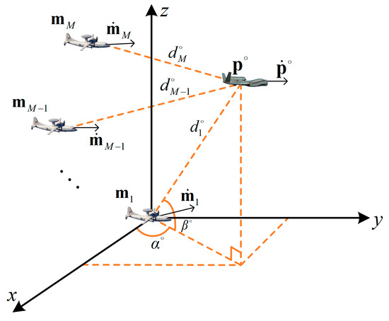
Figure 1.
The 3D localization scenarios.
Next, we derive the equations that relate the target parameters to the TDOA and FDOA. From the TDOA measurements, we obtain
where is the range difference (RD), which is the product of the TDOA and the signal propagation velocity, and can be expressed using the coordinates of the target as
To obtain the FDOA measurement formula, we take the derivative of both sides of (1) with respect to time, and the outcome is
where is the range difference rate (RDR), which can be calculated from FDOA measurements [18], and denotes the range rate, which is derived from Equation (2) for time:
Considering the error due to noise in the real situation, we make the measurement value the following:
where and . In addition, is the true RD vector, is the true RDR vector, and and are the measurement noise vectors.
We assume that and obey a Gaussian distribution with zero mean and , where is the covariance matrix of , and is the covariance matrix of .
3. The Proposed Location Method
Since the source range is unknown, inappropriate algorithms may be selected and result in suboptimal positioning performance. To solve this problem, referring to [23], this paper represents the position of the source as MPR coordinates to obtain a unified localization model. We introduce the velocity vector and denote the vector of the target parameters as , where is the azimuth angle of the target relative to the sensor , is the elevation angle of the target relative to the sensor , and is the inverse range between the target and the sensor and .
Squaring both sides of Formula (1) and combining it with formula (2), we obtain the TDOA equation [9]:
From Equation (6), we can see that the TDOA equation is only related to the position and not to the velocity , so we let (6) be derived with respect to time to obtain the FDOA equation:
To express the TDOA and FDOA equations using the MPR form, we can make and divide both sides of (6) and (7) by :
where is the unit vector of the pointing to the target, which has the expression
Then, substituting (5) into (8) and (9) and keeping only the linear error term, we can finally obtain the equations considering noise:
where , and represent noise error terms.
3.1. Unconstrained WLS
To design an estimation method for the nonlinear Equations (11) and (12), we define an auxiliary vector of size to turn the equations into linear equations and write the sets of measurement Equations (11) and (12) as a matrix:
where
Although we now have the linear matrix, Equation (13), the elements of the auxiliary vector have a nonlinear relationship with the target parameters, which can affect the estimation accuracy.
The derivation of the constraints is given below. Multiplying both sides of Equation (4) by gives the first constraint:
Moreover, according to the definition of , we can obtain the second constraint:
Thus, the localization problem is transformed into a WLS problem with two constraints:
where is the weighting matrix with the expression
and
Through (2) and (22), we can know that depends on the true parameters of the source, which are unknown. To solve this problem, we can make [18] and ignore the two constraints to solve for the unconstrained WLS estimate of :
From (23), we can obtain the parameters needed for . Then, we continue to solve for by substituting into (23), and so on several times to obtain a more accurate .
We assume that the measurement error in matrix is negligible, and then the covariance matrix of is
3.2. Optimization Algorithm Based on Constraints
3.2.1. Considering the First Constraint
This subsection uses the first constraint to reduce the estimation error of the previous step. We define a new auxiliary vector of size and express the auxiliary as the previous step estimate minus the error:
where is the estimation error term.
By expanding the first constraint in a first-order Taylor expansion [30], we obtain
Then, substituting (25) and (26) into (11) and (12) and combining the sets of measurement equations, we obtain the matrix equation
where
and the respective elements in the th row of and are
and the respective elements in the th row of and are
Using WLS to solve (25), we can obtain the error:
Therefore, the final estimate is obtained as
Similarly, we assume that the measurement error in matrix is negligible, and then the covariance matrix of (34) is
3.2.2. Considering the Second Constraint
In the previous subsection, we ignored the constraint on the unit vector . Since this constraint is only relevant for the DOA, this section uses this constraint to reduce the estimation results of from the previous step.
Defining as the true value plus the error value, we obtain
where is the error vector.
Substituting (36) into the second constraint and retaining the linear error term yields
Since is the first three elements of , Equation (37) can be rewritten as
where .
Through Equation (10), we know that
Then, by defining the vector and combining (38) and (39) to create the matrix, we can obtain the matrix
where
and
The WLS result of (40) is
where is the weighting matrix and
The calculation of requires the real parameters of the source, which can be derived with the help of the estimation results of the previous step since the parameter errors of the source obtained in the previous step are already small.
Finally, we can obtain the expression for the moving target parameter as
3.3. The Algorithmic Steps
In this subsection, we summarize the process of each step of the proposed method in this paper, as shown in Figure 2.
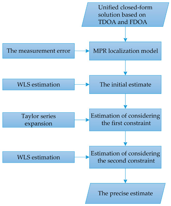
Figure 2.
The algorithmic flowchart.
4. Derivation of the CRLB
In this section, we present a detailed formulation of the CRLB under the model proposed in this paper. The CRLB is a lower bound describing the optimal performance of an unbiased estimator [31], which is defined as
where FIM is the Fisher information matrix and
where .
The partial derivative of with respect to is expressed as
From (1) and (4), we have
where .
Using (51), we can obtain
where
Using (52), we can obtain
where is
and from (64), we can obtain
With the above derivation, we end up with the . Substituting (49) into (48), we obtain the CRLB. The trace of the CRLB matrix is the minimum theoretical variance of the source parameters.
5. Numerical Simulations
In this section, we will verify the effectiveness of the proposed method through simulation. We use seven sensors, and their positions and velocities are shown in Table 1. For simplicity, we place the reference sensor at the origin. The covariance matrices are set to and , where is the variance of the measurement noise and is a matrix with diagonal elements of 1 and the rest of the elements of 0.5 [18,21]. To fully analyze the positioning performance, we use two evaluation metrics, mean square error (MSE) and bias, which are calculated as follows:
where is the number of Monte Carlo runs and is the estimation of the true value in the th Monte Carlo experiment.

Table 1.
Positions and speeds of sensors.
In this paper, two simulation scenarios are considered to estimate the target parameters based on target range variation and noise power variation, respectively. The algorithm presented in Section 3.2.1 of this paper is called OCWLS, and the algorithm after correcting the estimates in Section 3.2.2 is called TCWLS. Since all near-field localization algorithms in the Cartesian coordinate system have threshold effects, the classical Ho-TSWLS algorithm mentioned in [18] and the improved Ali-TSWLS algorithm mentioned in [21] are chosen as comparison algorithms. In addition, the CRLB is used as a standard for MSE estimation.
5.1. Impact of Source Range on Estimation Error
In this scenario, the target distance is increased from 10 to 200 km. The noise variance is and the angle of the source is randomly set to deg and deg. The variation in the DOA and inverse-range MSE estimations with increasing target distance is shown in Figure 3 and Figure 4. OCWLS and Ali-TSWLS have not achieved the CRLB, and their performance is approximately 2.7 dB above the CRLB. After using the optimized algorithm, we can observe that the localization performance is improved, with TCWLS reaching the CRLB and still maintaining an accurate estimation of the DOA at long range. However, the estimation of the DOA by Ho-TSWLS fails when the range increases to 120 km, and Ali-TSWLS fails when the range increases to 160 km due to the threshold effect. As seen in Figure 4, TCWLS also achieves the CRLB for the inverse-range MSE estimate. But Ho-TSWLS and Ali-TSWLS gradually increase starting from a km. Figure 5 shows the performance comparison of velocity MSE estimation with distance. When the km, Ho-TSWLS starts to deviate from the CRLB, while TCWLS stays close to the CRLB until the km. Ali-TSWLS is the best and stays close to the CRLB.
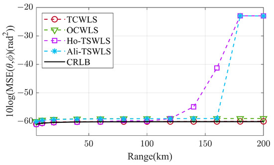
Figure 3.
Variation in MSE with distance for DOA estimate.
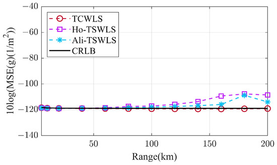
Figure 4.
Variation in MSE with distance for inverse-range estimate.
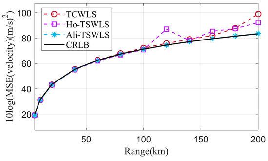
Figure 5.
Variation in MSE with distance for velocity estimate.
The variation in estimation bias with distance for the source parameters is shown in Figure 6, Figure 7 and Figure 8. For DOA estimation, the estimation bias of both OCWLS and TCWLS is much smaller than that of Ho-TSWLS and Ali-TSWLS, and TCWLS performs better than OCWLS, which is in line with the theoretical analysis. For inverse-distance estimation, the bias of TCWLS is much smaller than that of Ho-TSWLS and Ali-TSWLS, and Ali-TSWLS is about 3 dB lower than Ho-TSWLS. For speed estimation, the bias of the TCWLS and Ali-TSWLS methods is reduced by about 17 dB compared to Ho-TSWLS. The bias of TCWLS is lower than that of Ali-TSWLS up to 130 km, and beyond this point, the deviation of Ali-TSWLS becomes even lower. The results show that the proposed algorithm is equally effective for far-field targets, while Ho-TSWLS and Ali-TSWLS fail due to the threshold effect. Although Ali-TSWLS performs better for velocity estimation, it is poor for angle estimation.
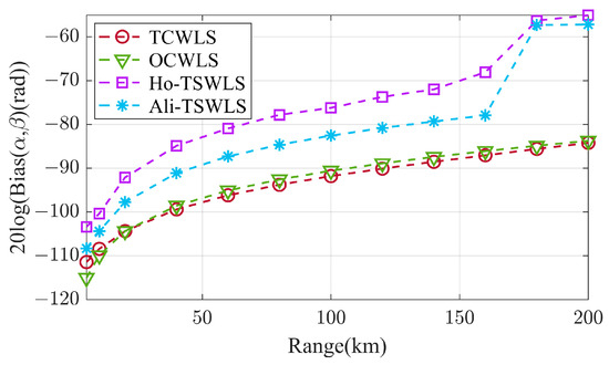
Figure 6.
Variation in bias with distance for DOA estimate.
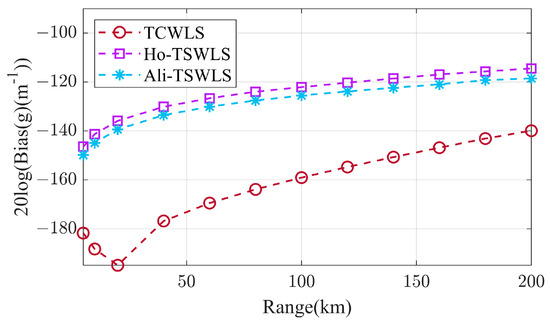
Figure 7.
Variation in bias with distance for inverse-range estimate.
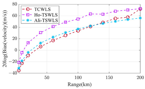
Figure 8.
Variation in bias with distance for velocity estimate.
Next, we transform the source parameters from MRP to the Cartesian coordinate system and compare the MSE and deviation of the source position to ensure the validity of the estimation of the target position. Figure 9 shows that before the distance reaches 160 km, the performance of all algorithms is equivalent, and the proposed algorithm begins to have a threshold effect when the km. This is caused by converting the inverse range into distance. A small inverse-range perturbation will cause a huge distance error, thus causing the position MSE to become larger. Although the MSE estimates of Ho-TSWLS and Ali-TSWLS are reasonable, they cannot provide an accurate DOA estimate. Figure 10 shows that TCWLS achieves the lowest deviation performance. We can conclude that TCWLS has the best bias performance in target location estimation, but sometimes the MSE performance may be degraded due to smaller inverse-range perturbations caused by excessively long distance or strong noise.

Figure 9.
Variation in MSE with distance for position estimate.
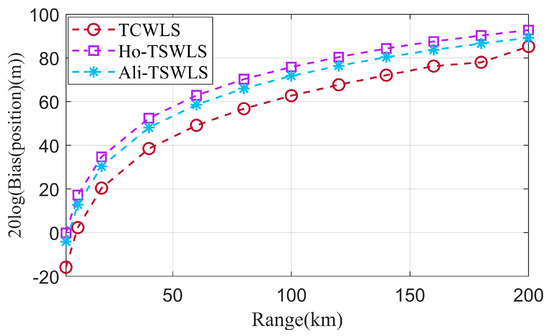
Figure 10.
Variation in bias with distance for position estimate.
5.2. Impact of Measurement Noise on Estimation Error
In the previous subsection, it is known that the proposed algorithm applies to far-field sources. In this subsection, we will analyze the effect of noise power on the positioning performance of the proposed algorithm in the near-field case. Noise power increased from -40 dB to 40 dB. The target is at a fixed distance of 15 km, with coordinates and speed .
Figure 11, Figure 12 and Figure 13 compare the MSE performance of several methods for target parameter estimation. For target angle estimation, OCWLS and TCWLS are consistently close to the CRLB, and OCWLS is about 2 dB higher than TCWLS. In contrast, Ho-TSWLS already deviates from the CRLB when , and Ali-TSWLS already deviates from the CRLB when . Similarly, TCWLS has stable performance for target inverse-range estimation, whereas Ho-TSWLS and Ali-TSWLS start to deteriorate in performance when . For speed estimation, TCWLS and Ho-TSWLS already deviate from the CRLB when , while Ali-TSWLS remains close to it until .
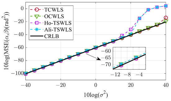
Figure 11.
Variation in MSE with noise power for DOA estimate.
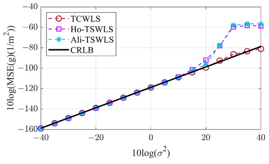
Figure 12.
Variation in MSE with noise power for inverse-range estimate.
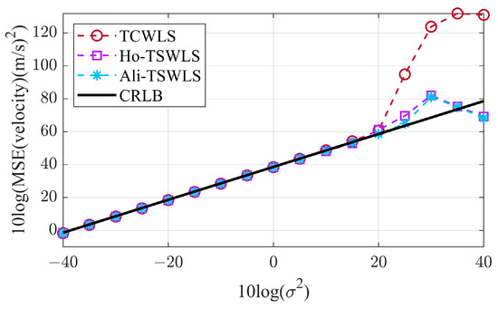
Figure 13.
Variation in MSE with noise power for velocity estimate.
Figure 14, Figure 15 and Figure 16 present the bias estimations. For DOA estimates, OCWLS and TCWLS are about 11 dB lower than Ho-TSWLS and about 6 dB lower than Ali-TSWLS. TCWLS has the best bias performance. For velocity estimation, TCWLS is about 19 dB lower than Ho-TSWLS when and about 4.5 dB lower than Ali-TSWLS when . However, Ali-TSWLS performance is best when .
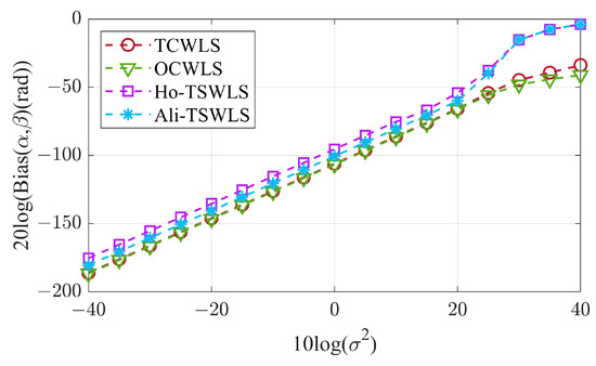
Figure 14.
Variation in bias with noise power for DOA estimate.
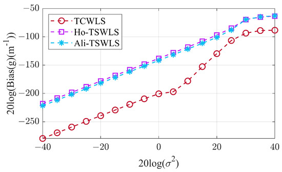
Figure 15.
Variation in bias with noise power for inverse-range estimate.
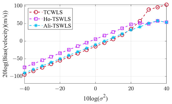
Figure 16.
Variation in bias with noise power for velocity estimate.
Next, the target parameters are transformed from MRP to a Cartesian coordinate system to compare the MSE and bias of the target location. Figure 17 shows that the performance of all algorithms is consistent when . However, the MSE estimates of the position of Ho-TSWLS and Ali-TSWLS are smaller when . The reason why the MSE of the proposed algorithm suddenly becomes larger was explained in Section 5.1 and will not be repeated here. Figure 18 compares the bias of all algorithms for position estimation and shows that TCWLS is the best when .
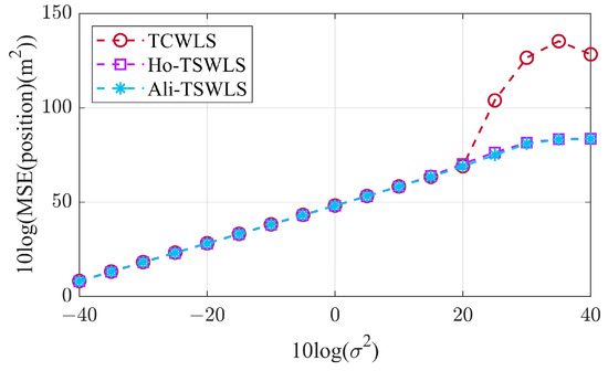
Figure 17.
Variation in MSE with noise power for position estimate.
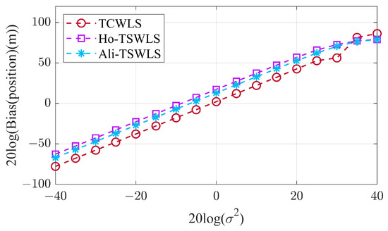
Figure 18.
Variation in bias with noise power for position estimate.
5.3. Computation Time
Finally, to compare the complexity of the algorithms, we calculated the average running time of several algorithms. Our simulation processing platform consists of a typical PC harnessing the power of an Intel i7-10700 CPU and a substantial 32.0 GB RAM. The equipment was sourced from Lenovo, in Beijing, China. It employs MATLAB R2021b as its software environment for executing the simulation processes. The simulation scenario is the one in Section 5.2, and the running time is shown in Table 2. Since several algorithms are closed-form solution algorithms, the running times are in the same order of magnitude, and the proposed algorithm has a slightly higher running time than Ho-TSWLS and Ali-TSWLS for the estimation of a moving target.
Table 2.
Average running time.
6. Discussion
This paper proposes a new moving target positioning method in three-dimensional space. The algorithm aims to locate the target without prior information of distance. The positions of the sensors in this paper are picked uniformly and randomly in three-dimensional space without having to maintain a certain configuration to be effectively localized. This can be successfully applied in complex scenarios.
From the simulation results, it can be concluded that under low noise power conditions, TCWLS can achieve the CRLB with a lower bias than the near-field Ho-TSWLS and Ali-TSWLS. However, it should be acknowledged that TCWLS first deviates from the CRLB for the velocity estimate as the noise power increases. This is the direction we need to continue to study in the future. In addition, we need to be aware that small perturbations in the distance inverse estimate can cause large distance and position estimation errors in far-field or strongly noisy power situations. As shown in Equation (46), if the azimuth or elevation angles are at certain specific angles, such as deg, this can cause the weighting matrix to become a singular matrix affected by , ultimately leading to poor positioning performance. This can be avoided by selecting a different sensor as the reference sensor.
TCWLS can also be used in two-dimensional space by simplifying the equations. Furthermore, it can also be used with slight modifications if sensor parameter errors need to be considered.
7. Conclusions
We propose a new positioning algorithm that does not require prior distance knowledge of the moving target. For a near-field target, we can accurately estimate the location and velocity of the target. For a far-field target, we can accurately estimate the DOA of the target. The method first builds a unified model using MPR, then creates an optimization problem with two constraints, and finally obtains an exact closed-form solution via WLS and an optimization algorithm. Simulation experiments validate that the proposed unified localization approach is superior to the traditional near-field moving target localization method. Our future work will focus on improving the robustness of the proposed algorithm in strong noise environments.
Author Contributions
Conceptualization, W.G. and X.S.; methodology, W.G. and X.S.; software, W.G. and X.S.; validation, W.G. and X.S.; formal analysis, W.G. and C.Z.; investigation, C.Z. and Q.W.; resources, W.G.; data curation, W.G. and C.Z.; writing—original draft preparation, W.G. and X.S.; writing—review and editing, Q.W. and Y.L.; visualization, X.S.; supervision, Q.W.; project administration, Q.W.; funding acquisition, Y.L. All authors have read and agreed to the published version of the manuscript.
Funding
This research was funded by the National Natural Science Foundation of China, grant numbers 62171337, 62201434, 62101396, and 62301391, and supported by the Postdoctoral Fellowship Program of CPSF under Grant Number GZC20233512.
Data Availability Statement
Data are contained within the article.
Acknowledgments
The authors would like to thank all editors and reviewers for their valuable comments and suggestions.
Conflicts of Interest
The authors declare no conflicts of interest.
References
- Weinstein, E. Optimal source localization and tracking from passive array measurements. IEEE Trans. Acoust. Speech Signal Process. 1982, 30, 69–76. [Google Scholar] [CrossRef]
- Rappaport, T.S.; Reed, J.H.; Woerner, B.D. Position location using wireless communications on highways of the future. IEEE Commun. Mag. 1996, 34, 33–41. [Google Scholar] [CrossRef]
- Flückiger, M.; Neild, A.; Nelson, B.J. Optimization of receiver arrangements for passive emitter localization methods. Ultrasonics 2012, 52, 447–455. [Google Scholar] [CrossRef]
- Indelman, V.; Gurfil, P.; Rivlin, E. Real-Time Vision-Aided Localization and Navigation Based on Three-View Geometry. IEEE Trans. Aerosp. Electron. Syst. 2012, 48, 2239–2259. [Google Scholar] [CrossRef]
- Le, T.-K.; Ono, N. Closed-Form and Near Closed-Form Solutions for TDOA-Based Joint Source and Sensor Localization. IEEE Trans. Signal Process. 2017, 65, 1207–1221. [Google Scholar] [CrossRef]
- Chan, Y.T.; Tsui, W.Y.; So, H.C.; Ching, P.C. Time-of-Arrival Based Localization Under NLOS Conditions. IEEE Trans. Veh. Technol. 2006, 55, 17–24. [Google Scholar] [CrossRef]
- Junyang, S.; Molisch, A.F.; Salmi, J. Accurate Passive Location Estimation Using TOA Measurements. IEEE Trans. Wireless Commun. 2012, 11, 2182–2192. [Google Scholar] [CrossRef]
- Nguyen, N.H.; Dogancay, K. Optimal Geometry Analysis for Multistatic TOA Localization. IEEE Trans. Signal Process. 2016, 64, 4180–4193. [Google Scholar] [CrossRef]
- Chan, Y.T.; Ho, K.C. A simple and efficient estimator for hyperbolic location. IEEE Trans. Signal Process. 1994, 42, 1905–1915. [Google Scholar] [CrossRef]
- Xu, E.; Ding, Z.; Dasgupta, S. Source Localization in Wireless Sensor Networks From Signal Time-of-Arrival Measurements. IEEE Trans. Signal Process. 2011, 59, 2887–2897. [Google Scholar] [CrossRef]
- Ho, K.C. Bias Reduction for an Explicit Solution of Source Localization Using TDOA. IEEE Trans. Signal Process. 2012, 60, 2101–2114. [Google Scholar] [CrossRef]
- Malanowski, M.; Kulpa, K. Two_Methods_for_Target_Localization_in_Multistatic_Passive_Radar. IEEE Trans. Aerosp. Electron. Syst. 2012, 48, 572–580. [Google Scholar] [CrossRef]
- Dogancay, K. Emitter localization using clustering-based bearing association. IEEE Trans. Aerosp. Electron. Syst. 2005, 41, 525–536. [Google Scholar] [CrossRef]
- Wang, Y.; Ho, K.C. An Asymptotically Efficient Estimator in Closed-Form for 3-D AOA Localization Using a Sensor Network. IEEE Trans. Wireless Commun. 2015, 14, 6524–6535. [Google Scholar] [CrossRef]
- Zheng, Y.; Sheng, M.; Liu, J.; Li, J. Exploiting AoA Estimation Accuracy for Indoor Localization: A Weighted AoA-Based Approach. IEEE Wireless Commun. Lett. 2019, 8, 65–68. [Google Scholar] [CrossRef]
- Wang, G.; Yang, K. A New Approach to Sensor Node Localization Using RSS Measurements in Wireless Sensor Networks. IEEE Trans. Wireless Commun. 2011, 10, 1389–1395. [Google Scholar] [CrossRef]
- Feng, C.; Au, W.S.A.; Valaee, S.; Tan, Z. Received-Signal-Strength-Based Indoor Positioning Using Compressive Sensing. IEEE Trans. Mob. Comput. 2012, 11, 1983–1993. [Google Scholar] [CrossRef]
- Ho, K.C.; Xu, W. An Accurate Algebraic Solution for Moving Source Location Using TDOA and FDOA Measurements. IEEE Trans. Signal Process. 2004, 52, 2453–2463. [Google Scholar] [CrossRef]
- Yu, H.; Huang, G.; Gao, J.; Liu, B. An Efficient Constrained Weighted Least Squares Algorithm for Moving Source Location Using TDOA and FDOA Measurements. IEEE Trans. Wireless Commun. 2012, 11, 44–47. [Google Scholar] [CrossRef]
- Qu, X.; Xie, L.; Tan, W. Iterative Constrained Weighted Least Squares Source Localization Using TDOA and FDOA Measurements. IEEE Trans. Signal Process. 2017, 65, 3990–4003. [Google Scholar] [CrossRef]
- Noroozi, A.; Oveis, A.H.; Hosseini, S.M.; Sebt, M.A. Improved Algebraic Solution for Source Localization from TDOA and FDOA Measurements. IEEE Wireless Commun. Lett. 2018, 7, 352–355. [Google Scholar] [CrossRef]
- Sun, Y.; Ho, K.C.; Wan, Q. Solution and Analysis of TDOA Localization of a Near or Distant Source in Closed Form. IEEE Trans. Signal Process. 2019, 67, 320–335. [Google Scholar] [CrossRef]
- Wang, Y.; Ho, K.C. TDOA Positioning Irrespective of Source Range. IEEE Trans. Signal Process. 2017, 65, 1447–1460. [Google Scholar] [CrossRef]
- Sun, Y.; Ho, K.C.; Wang, G.; Chen, H.; Yang, Y.; Chen, L.; Wan, Q. Computationally Attractive and Location Robust Estimator for IoT Device Positioning. IEEE Internet Things J. 2022, 9, 10891–10907. [Google Scholar] [CrossRef]
- Wang, G.; Ho, K.C. Convex Relaxation Methods for Unified Near-Field and Far-Field TDOA-Based Localization. IEEE Trans. Wireless Commun. 2019, 18, 2346–2360. [Google Scholar] [CrossRef]
- Wang, Y.; Ho, K.C. Unified Near-Field and Far-Field Localization for AOA and Hybrid AOA-TDOA Positionings. IEEE Trans. Wireless Commun. 2018, 17, 1242–1254. [Google Scholar] [CrossRef]
- Sun, Y.; Ho, K.C.; Wan, Q. Eigenspace Solution for AOA Localization in Modified Polar Representation. IEEE Trans. Signal Process. 2020, 68, 2256–2271. [Google Scholar] [CrossRef]
- Chen, X.; Wang, G.; Ho, K.C. Semidefinite relaxation method for unified near-Field and far-Field localization by AOA. Signal Process. 2021, 181, 107916. [Google Scholar] [CrossRef]
- Wang, G.; Xiao, Y.; Ho, K.C.; Huang, L. Unified Near-Field and Far-Field TDOA Source Localization Without the Knowledge of Signal Propagation Speed. IEEE Trans. Commun. 2024, 72, 2166–2181. [Google Scholar] [CrossRef]
- Zhang, F.; Sun, Y.; Zou, J.; Zhang, D.; Wan, Q. Closed-Form Localization Method for Moving Target in Passive Multistatic Radar Network. IEEE Sensors J. 2020, 20, 980–990. [Google Scholar] [CrossRef]
- Kay, S.M. Fundamentals of Statistical Signal Processing: Estimation Theory, 1st ed.; Prentice-Hall: Englewood Cliffs, NJ, USA, 1993. [Google Scholar]
Disclaimer/Publisher’s Note: The statements, opinions and data contained in all publications are solely those of the individual author(s) and contributor(s) and not of MDPI and/or the editor(s). MDPI and/or the editor(s) disclaim responsibility for any injury to people or property resulting from any ideas, methods, instructions or products referred to in the content. |
© 2024 by the authors. Licensee MDPI, Basel, Switzerland. This article is an open access article distributed under the terms and conditions of the Creative Commons Attribution (CC BY) license (https://creativecommons.org/licenses/by/4.0/).