Visual Localization Method for Unmanned Aerial Vehicles in Urban Scenes Based on Shape and Spatial Relationship Matching of Buildings

Abstract

In urban scenes, buildings are usually dense and exhibit similar shapes. Thus, existing autonomous unmanned aerial vehicle (UAV) localization schemes based on map matching, especially the semantic shape matching (SSM) method, cannot capture the uniqueness of buildings and may result in matching failure. To solve this problem, we propose a new method to locate UAVs via shape and spatial relationship matching (SSRM) of buildings in urban scenes as an alternative to UAV localization via image matching. SSRM first extracts individual buildings from UAV images using the SOLOv2 instance segmentation algorithm. Then, these individual buildings are subsequently matched with vector e-map data (stored in .shp format) based on their shape and spatial relationship to determine their actual latitude and longitude. Control points are generated according to the matched buildings, and finally, the UAV position is determined. SSRM can efficiently realize high-precision UAV localization in urban scenes. Under the verification of actual data, SSRM achieves localization errors of 7.38 m and 11.92 m in downtown and suburb areas, respectively, with better localization performance than the radiation-variation insensitive feature transform (RIFT), channel features of the oriented gradient (CFOG), and SSM algorithms. Moreover, the SSRM algorithm exhibits a smaller localization error in areas with higher building density.

1. Introduction

Owing to the small size and suitable flexibility of unmanned aerial vehicles (UAVs), their application fields are constantly expanding, and they are now widely employed in map surveying and mapping, emergency search and rescue, and military reconnaissance fields. Accurate positioning is a prerequisite for UAVs to realize precise control and mission execution. A global navigation satellite system (GNSS) provides a universal localization method for UAVs. However, GNSS signals readily exhibit interference in complex electromagnetic environments, where the localization accuracy and reliability are substantially affected [1,2]. Therefore, it is necessary to assist UAVs in obtaining localization information by other means.

UAVs generally carry small, low-cost vision sensors when performing tasks; thus, vision-based localization methods are generally used to replace or as a supplement to GNSS [3,4]. In the vision-based localization method, vision sensors carried by UAVs are used to sense the environment, after which the position of the UAVs can be estimated upon image information processing and analysis. Vision-based localization methods do not rely on external signals and provide the advantage of high anti-interference ability [5,6]. For outdoor scenes, the absolute visual localization method based on image matching is the most commonly employed method. The basic principle of vision-based localization is to match real-time UAV images with geo-referenced data, which are usually pre-collected UAV images or satellite remote sensing images. Then, the latitude and longitude corresponding to each pixel of the UAV images can be obtained, and finally, the UAV position can be determined [1,7]. Image matching methods, such as the mutual information (MI) and scale-invariant feature transform (SIFT) methods, generally involve the use of grayscale and texture features to describe image similarity [8,9], leading to failure when there are temporal, imaging perspective, and lighting condition differences between the geo-referenced images and UAV images.

To address the above challenges, a few researchers have proposed the use of map-based matching methods to achieve UAV localization. For example, Nassar [10] considered the shape and area information of individual buildings to match UAV images and a map produced from geo-referenced images, referred to as semantic shape matching (SSM). Map-based matching methods can overcome the differences in color and lighting between UAV images and geo-referenced data [11]. However, the existing map-based matching methods entail the use of geo-referenced maps produced from remote sensing images, which indicates that these maps may not be accurate. Moreover, buildings within a given city are often dense and exhibit similar shapes. Thus, the use of the shape and area of buildings alone cannot capture their uniqueness. Therefore, prior methods can hardly match individual buildings in urban scenes.

According to theory in the field of geographic information science, the most accurate feature of a spatial scene is the spatial relationship [12], and the spatial distribution of buildings can uniquely characterize a given scene. To address the issue of insufficient feature descriptions and the possible failure of existing map-based matching methods, we propose a novel autonomous UAV localization method for urban scenes based on the shape and spatial relationship matching (SSRM) of buildings in urban scenes. The main contributions of our study are as follows:

(1)

In SSRM, vector e-map data (stored in .shp format) are used as geo-referenced data instead of pre-collected images or image-based map-related data. The e-map data can comprehensively reflect the individual and spatial relationship characteristics of buildings while also reducing the amount of data prestored on UAVs.

(2)

We propose a scene matching method in which the shape information and spatial relationships of buildings are used to match UAV images and geo-referenced data. Compared with existing map-based matching methods, increased consideration is given to the spatial relationships between buildings, thus greatly enhancing the robustness of the matching process.

(3)

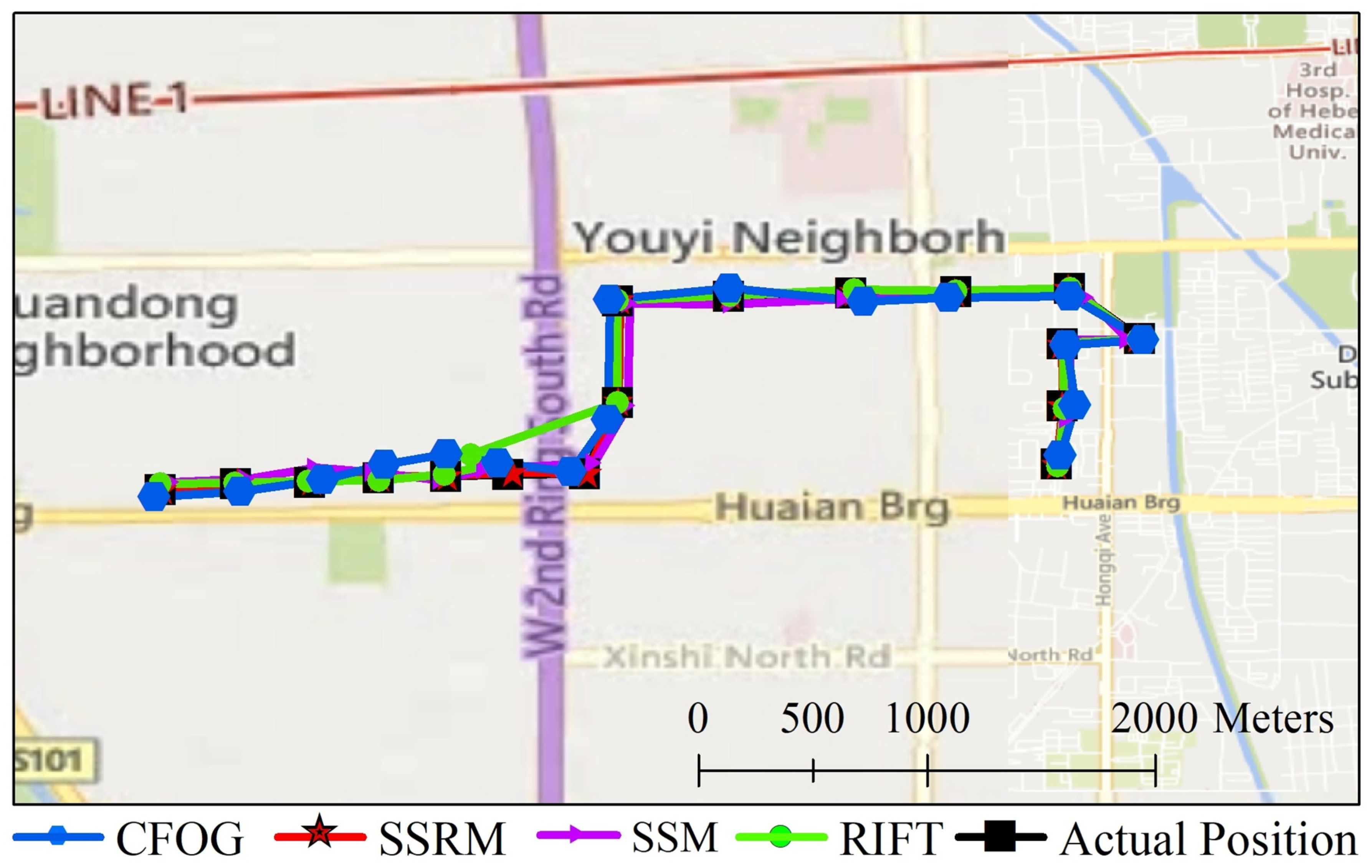
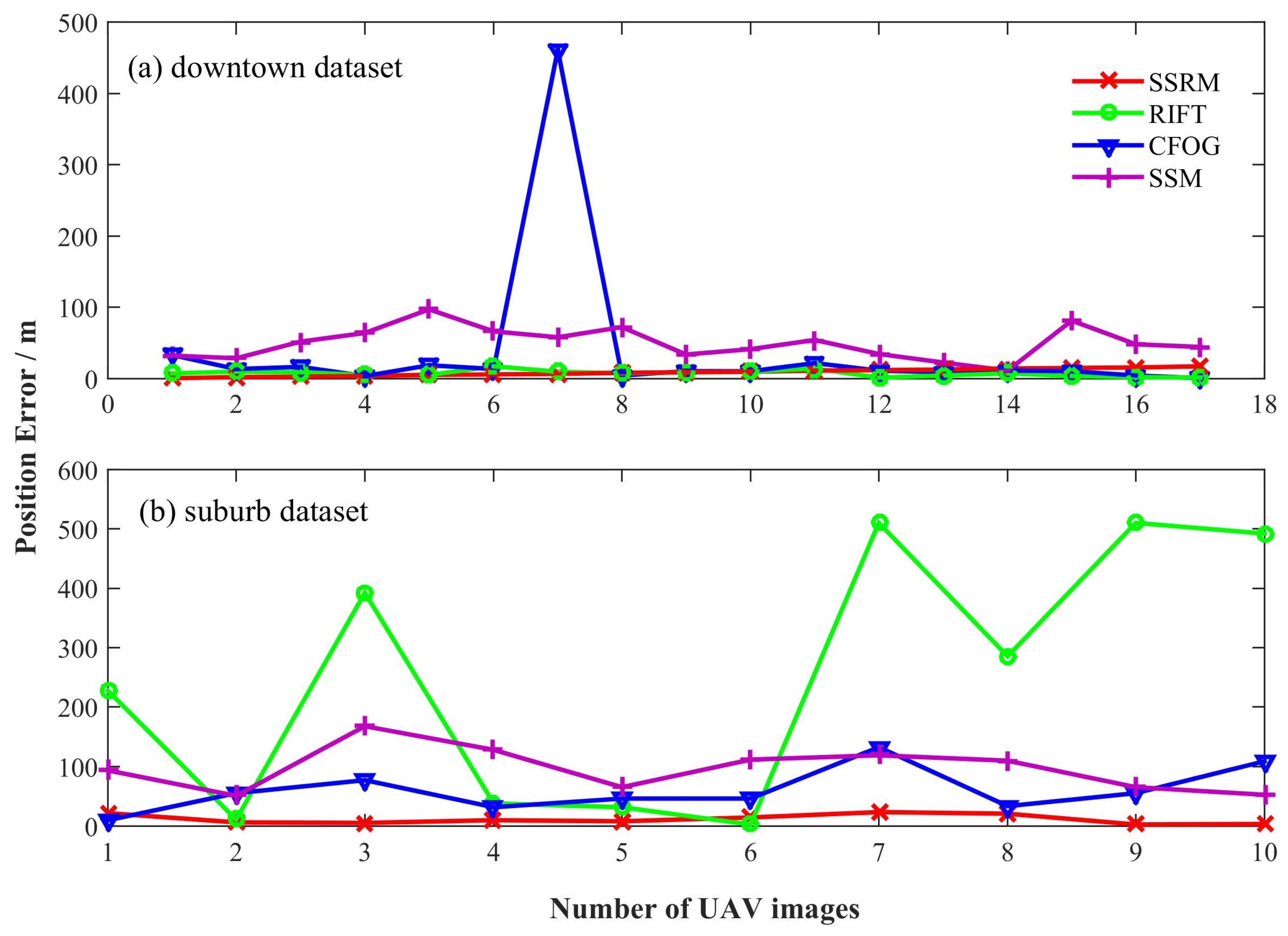
The effectiveness of the SSRM method is verified via simulation flight data. Moreover, we compare the SSRM method with the radiation-variation insensitive feature transform (RIFT) feature matching algorithm [13], the channel features of oriented gradient (CFOG) template matching algorithm [14], and the SSM map-based algorithm [10]. The consideration of the shape and spatial relationships of buildings ensures the accuracy of scene matching and provides far better localization accuracy.

The remainder of the article is organized as follows: In Section 2, related works are introduced. Our method is described in detail in Section 3. Section 4 presents the datasets and experiments used to validate our method. Section 5 provides the validation results and the comparative experimental results. The factors that may introduce errors are discussed in Section 6. Finally, conclusions are noted, and future research directions are outlined in Section 7.

2. Related Works

Absolute visual localization methods are classified into two categories according to the geo-referenced data used for matching UAV images: image-based matching methods and map-based matching methods.

2.1. Image-Based Matching Methods

Image-based matching methods generally involve the use of high-resolution satellite remote sensing images or pre-collected UAV images with geographic coordinates as geo-referenced images, and UAV images are matched with geo-referenced images. The different image matching algorithms can be subcategorized into template matching methods, feature matching methods, and deep learning-based matching methods.

2.1.1. Template Matching Methods

Template matching methods typically entail the use of robust similarity metrics to evaluate image similarity within a predefined window. Grayscale information within the window is usually employed to compute the similarity metric [15]. In template matching, it is usually assumed that there is a slight difference in appearance between the UAV and geo-referenced images, so the sum of squared differences (SSD) and normalized cross correlation (NCC) are often adopted as standard matching templates [16,17]. However, there are inevitably temporal differences, illumination differences, and imaging perspective differences between UAV images and geo-referenced images, which usually lead to the failure to match UAV images with geo-referenced images [1]. The MI method is more robust to radiometric differences and can resist nonlinear grayscale distortion, and this method aims to calculate the mutual information value in the search window between the UAV images and geo-referenced images [18].

In addition to using grayscale information to calculate the template similarity metric, the geometric structure and morphological features can be used to characterize the similarity between images. For projecting and quantizing histograms of oriented gradients (PQ-HOG) algorithms [19], oriented gradients are used as the basic similarity metric. Moreover, the phase congruency (PC) exhibits greater resistance to illumination and contrast variations, so the histogram of oriented phase congruency (HOPC) method utilizes phase congruency intensity and orientation information to construct similarity descriptors [20]. On the basis of the HOPC method, the CFOG method extracts local descriptors at each pixel to form a pixelwise feature representation, and fast Fourier transform (FFT) is used to define a fast similarity measure in the frequency domain for improving the computational efficiency [14]. The CFOG method has been successfully applied in multiple commercial software programs and has been demonstrated to achieve higher matching accuracy than does the HOPC method [21].

When land cover change occurs between the UAV and geo-referenced image, the above methods may fail. In addition, template matching methods usually require iteration of the geo-referenced image to calculate the similarity within different windows, after which the window with the greatest similarity can be selected as the matching result, thus requiring intensive computations.

2.1.2. Feature Matching Methods

Feature matching methods do not search the whole image but extract representative feature points, so the number of computations is greatly reduced [22]. However, seasonal or color differences between the UAV and geo-referenced images usually lead to the failure of classical feature operators, such as the SIFT, ORB, and SURF operators. Therefore, researchers have proposed image matching schemes that are independent of image color differences. Mantelli et al. proposed the abBRIEF operator, which aims to use the CIE color space to match UAV and geo-referenced images [23]. Ye et al. constructed a feature detector, namely, the minimum moment of phase congruency (MMPC)-Lap method, to robustly determine luminance and contrast variations [20]. Li et al. proposed the RIFT method, using PC for feature point detection and the maximum index map (MIM) for feature description, which makes it unsensitive to nonlinear radiation distortions [13].

In noncooperative areas, high-resolution satellite remote sensing images are usually used as geo-referenced images, and the scale and color differences between UAV and geo-referenced images are generally obvious. In addition, when there are imaging perspective differences between the UAV and geo-referenced images, the complex three-dimensional structure within a city can lead to different areas of exposure for buildings, and a land object can exhibit varying appearances. Therefore, feature matching methods typically yield more mismatched points and a poorer performance.

2.1.3. Deep Learning-Based Matching Methods

Compared with template matching and feature matching methods, deep learning-based methods provide superior learning and representation capabilities for deep features of images and provide obvious advantages in scene adaptation and robustness. Initially, deep learning-based methods were used to extract more representative feature points, which were then combined with traditional similarity metrics to increase the image alignment accuracy [24,25]. Thereafter, research gradually shifted to end-to-end image matching. Danial et al. proposed a self-supervised image matching framework, SuperPoint, which first utilized feature points of simple geometric shapes (e.g., triangles, rectangles) in a synthetic dataset to train a pre-trained detector, namely, MagicPoint. The homographic adaptation module was subsequently used to help relate the feature points across different perspectives and scales to increase the feature point redetection rate and the cross-domain utility [26]. Sarlin et al. proposed a network, namely, SuperGLUE, that can simultaneously perform feature matching and nonmatching point filtering. In SuperGLUE, a graph neural network (GNN) is used to predict the loss function of matching, solve the differentiable optimal transport problem, and ultimately realize feature matching. Moreover, SuperGLUE uses a flexible content aggregation mechanism based on the attention mechanism, which enables it to perceive potential 3D scenes and perform feature matching [27]. Inspired by the SuperGLUE architecture, Sun et al. proposed a new detector-free local image feature matching method, namely, LoFAR. In the LoFAR method, a transformer with self- and cross-attention layers is employed to obtain the feature descriptors of two images. Dense matching is achieved at the coarse-grained level, and dense matching is subsequently refined at the subpixel level [28].

The SuperPoint, SuperGLUE, and LoFAR methods are widely used in simultaneous localization and mapping (SLAM), which also indicates that they require that the matched images exhibit the same size. In outdoor image matching, UAV images and geo-referenced data are always of different sizes, and iteration of the whole geo-referenced image for matching with the UAV image is needed. Furthermore, deep learning-based methods require numerous samples for training, and many geo-referenced images must be stored on UAVs in advance, especially for large flight areas.

2.2. Map-Based Matching Methods

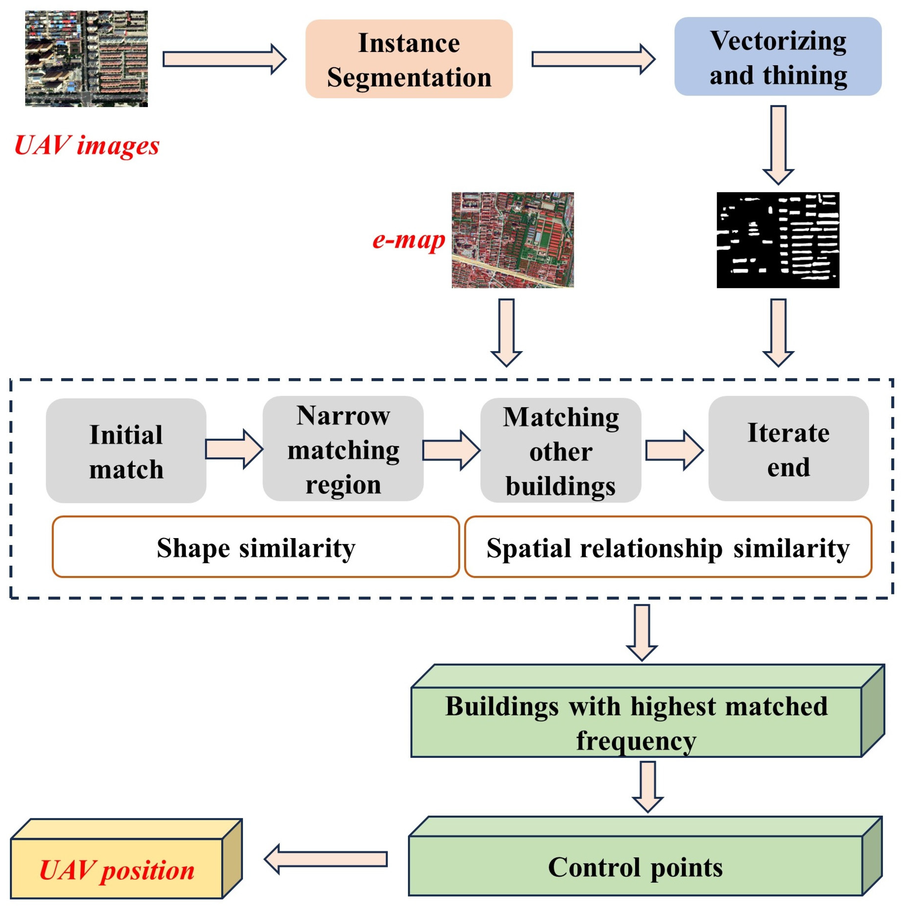
Instead of using pre-collected or satellite remote sensing images as geo-referenced data, maps reflecting land cover are used in map-based matching methods.

UAV images may exhibit different colors due to weather and temporal differences, but the land cover type rarely changes. Therefore, land cover data can be used as geo-referenced data. Masselli et al. employed land cover classification results from Google Earth images as geo-referenced data [29]; during flight, the collected images were classified to land cover and matched with the aforementioned geo-referenced map. Choi proposed a building ratio map (BRM) method, in which the building layer from pre-collected remote sensing images is applied as geo-referenced data. In the BRM method, the ratio of buildings within circles with different radii is determined to produce feature vectors, which are then used to estimate the similarity between UAV images and the building layer for retrieving candidate UAV flight areas [11]. Hao et al. abstracted buildings as point clouds, which could be further regarded as geo-referenced data to match UAV images via a point cloud matching algorithm [30]. Wang et al. reported that the shadow map is a stable feature for scene matching navigation and proposed a shadow-based matching method for the localization of low-altitude flight UAVs [31].

Currently, only a few studies have focused on map-based matching, and there is no unanimously recognized scheme. Moreover, existing methods still entail the use of pre-collected remote sensing images as geo-referenced data, which introduces additional errors.

3. Methodology

In the absence of GNSS signals, if the takeoff position of the UAV is known, the inertial navigation system (INS) can provide rough location information for the UAV within a certain period. The flight altitude of the UAV is generally derived from barometric altimeters. Furthermore, the internal parameters of the camera are known, so the spatial resolution of the UAV images can be calculated directly. The magnetometer can provide UAV flight orientation information. Thus, UAV images can be geometrically corrected with flight orientation information [32,33]. When the camera is at the real nadir, the latitude and longitude of the central pixel of an image reflect the UAV position.

If the takeoff position, spatial resolution, and orientation of UAV images are known, our method first extracts the roof outlines of individual buildings from UAV images, after which they are matched with building entities in the e-map based on their shape and spatial relationship. The buildings with the highest matched frequency can be used to generate control points accordingly, which ultimately can be applied to determine the UAV position. The overall flow is shown in Figure 1.

If the UAV location at takeoff is also unknown, then as long as the city where the UAV is located is known and a rough location is manually specified for the UAV, SSRM takes more time only in the first matching. And once the approximate position of the UAV at a certain moment is determined, the matching range can be narrowed down.

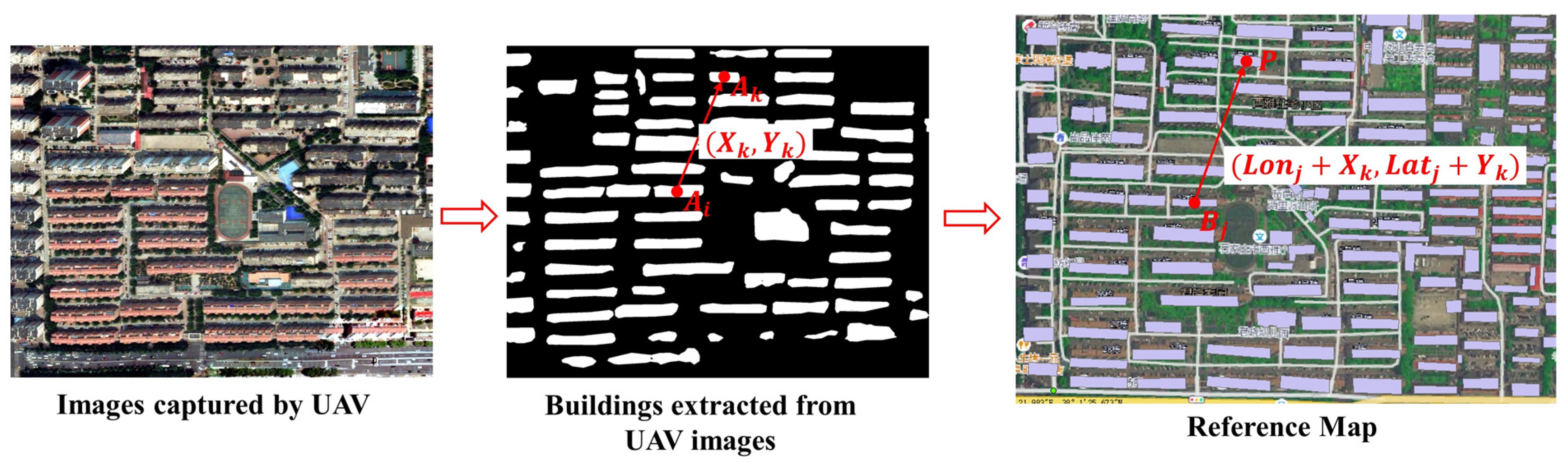
3.1. Individual Building Extraction

The instance segmentation algorithm not only exhibits the characteristics of semantic segmentation (for pixel-level classification and effective outline extraction) but also exhibits the characteristics of target detection (for distinguishing and locating different individuals of the same category). Therefore, the instance segmentation algorithm is generally selected to extract individual buildings from remote sensing images. Owing to the need for fast image interpretation in UAV localization and considering that the buildings in UAV images are almost always large targets, we use the SOLOv2 model for individual building extraction, thereby relying on its efficiency and favorable instance segmentation ability for large targets [34,35]. The SOLOv2 model, based on the SOLO architecture, uses ResNet101 trained on the ImageNet dataset as the backbone network to extract features. And then, the feature pyramid network (FPN) outputs feature maps of different sizes as inputs for the prediction head, which divides the input feature maps into S × S grids. If the center of the object falls within a grid cell, the grid is responsible for (1) predicting the semantic category by a category branch and (2) segmenting the object instance by a mask branch. Finally, the SOLOv2 model uses matrix non-maximum suppression (NMS) to parallelize the NMS, which renders it advantageous in terms of both its speed and accuracy.

Implementation Details. We use the SOLOv2 model under the MMDetection framework. Multiscale sampling and random flipping are employed for image enhancement during training to adapt to buildings with varying scales at different spatial resolutions. The base learning rate is set to 0.01 with a weight decay of 0.0001 and a momentum of 0.9. The Dice coefficient, which is a metric used to estimate the similarity between the image segmentation results and ground-truth data, is adopted as the loss function of the mask branch. The Dice coefficient represents the degree of overlap between the image segmentation target and the ground truth. The maximum number of iteration epochs is set to 5000 for training.

After extracting the individual buildings from UAV images, the buildings are converted into outline information and stored in the form of image coordinate strings. To reduce the computational burden for subsequent scene matching, the building outlines are thinned via the Douglas–Peucker algorithm [36]. Furthermore, individual buildings with areas smaller than 50 pixels are removed. Considering that the UAV orientation and flight altitude are known, the resolution of the images can be estimated, and the central pixel coordinates, actual area, and aspect ratio of the minimum bounding rectangle for all buildings can be calculated.

3.2. Scene Matching and UAV Position Determination

It is necessary to determine the scene of UAV images before the UAV spatial location can be obtained, which suggests the matching of semantic information interpreted from the UAV images with the e-map to determine which building within the geographic space corresponds to the building in the UAV images. Owing to the complexity of urban scenes and the high frequency of similar buildings, it is unreliable to use only the shape features of buildings for scene matching, such as in SSM [10]. Spatial scenes are most accurately characterized by spatial relationships rather than the shape and size of targets [12]. Therefore, we design a vector scene matching method based on the shape and spatial relationships of individual buildings, and the basic concept of this approach is shown in Figure 2.

Assuming that the UAV localization uncertainty is R = 500 m, A is the UAV image, and Map denotes the geo-referenced map, then the longest side length of each UAV image is r. The process of matching A and Map is as follows:

(1) Iterate over building individuals A_i (1 ≤ i ≤ N) extracted from UAV images.

(2) Using the initial position of the UAV as the center and a radius of (R + r) m, perform a spatial retrieval on Map, and the retrieval result is B. The central geographic coordinates of the buildings B_j (1 ≤ j ≤ M) in B are denoted as (Lon_j, Lat_j).

(3) Compute the Euclidean distances (spatial resolution × pixel distance) of the central pixel (x_i, y_i) of A_i from the four boundaries of the current UAV image. The distance between A_i and the upper boundary is L_t, the distance from the lower boundary is L_b, the distance from the left boundary is L_l, and the distance from the right boundary is L_r.

(4) Iterate over B_j. If the area ratio of B_j to A_i AreaRatio(B_j, A_i) and the minimum bounding rectangle aspect ratio of B_j to A_i AspectRatio(B_j, A_i) satisfy the following relationship:

$$0.5\le AreaRatio(B_j,A_i)\le 2$$

(1)

$$0.5\le AspectRatio(B_j,A_i)\le 2$$

(2)

then, B_j matches A, and proceed to the next step. Otherwise, continue iterating over B_j.

(5) With B_j as the center, construct the buffer zone along four directions in B. The buffer distance on the north side is L_t, the buffer distance on the south side is L_b, the buffer distance on the west side is L_l, and the buffer distance on the east side is L_r. The buildings within the buffer zone constitute the final candidate map to be matched.

(6) Calculate the Euclidean vector distance (X_k, Y_k) between the central pixel of each A_k(k ≠ i) and the central pixel of A_i and apply the spatial analysis technique to determine whether point P(Lon_j + X_k, Lat_j + Y_k) is located in a building on the candidate map. If not, there is no matching building for A_i, and if P is located in building B_c on the candidate map, we further determine whether the following relationships between A_k and B_c are satisfied:

$$0.5\le AreaRatio(B_c,A_k)\le 2$$

(3)

$$0.5\le AspectRatio(B_c,A_k)\le 2$$

(4)

If the above relationships hold, $B_c$ is considered successfully matched with $A_k$, and the number of matches is increased by one. Otherwise, $A_k$ is not associated with a matching building.

Finally, the frequency of successfully matched pairs of buildings in A and B is counted, and the top N (N ≤ 15) pairs of (A_m, B_m) with matched frequencies greater than 3 are adopted as the final successfully matched pairs. Considering the uncertainty in the instance segmentation algorithm when extracting building outlines, we assume that the central coordinates of the successfully matched A_m(x_m, y_m) and B_m(Lon_m, Lat_m) are the ground control point pairs. When the UAV camera is at the real nadir, the geographic coordinates corresponding to the central pixel of the image are the geographic coordinates of the UAV. Therefore, as expressed in Equations (5)–(10), the geographic coordinate of the central pixel of the UAV image can be calculated via a linear regression algorithm, and control points with an error greater than 2 times the standard deviation are excluded in the regression process:

$$b={\displaystyle \frac{\sum _{m=1}^{15}({Lat}_m-\overline{Lat})(y_m-\overline{y})}{\sum _{m=1}^{15}{(y_m-\overline{y})}^2}}$$

(5)

$$a=\overline{Lat}-b\overline{y}$$

(6)

$${Lat}_{center}=b{y}_{center}+a$$

(7)

$$d={\displaystyle \frac{\sum _{m=1}^{15}({Lon}_m-\overline{Lon})(x_m-\overline{x})}{\sum _{m=1}^{15}{(x_m-\overline{x})}^2}}$$

(8)

$$c=\overline{Lon}-b\overline{x}$$

(9)

$${Lon}_{center}=d{x}_{center}+c$$

(10)

where a, b, c, and d are the coefficients of the linear equation between the geographic coordinates and the image pixel coordinates; Lat_m and Lon_m are the central geographic coordinates of the successfully matched building in the e-map; $\overline{Lat}$ and $\overline{Lon}$ are the mean values of Lat_m and Lon_m, respectively; $x_m$ and $y_m$ are the central pixel coordinates of the successfully matched buildings in the UAV image; $\overline{x}$ and $\overline{y}$ are the mean values of $x_m$ and $y_m$, respectively; $x_{center}$ and $y_{center}$ are the central pixel coordinates of the UAV image; and ${Lat}_{center}$ and ${Lon}_{center}$ are the geographic coordinates corresponding to the center of the UAV image.

4. Data and Experiments

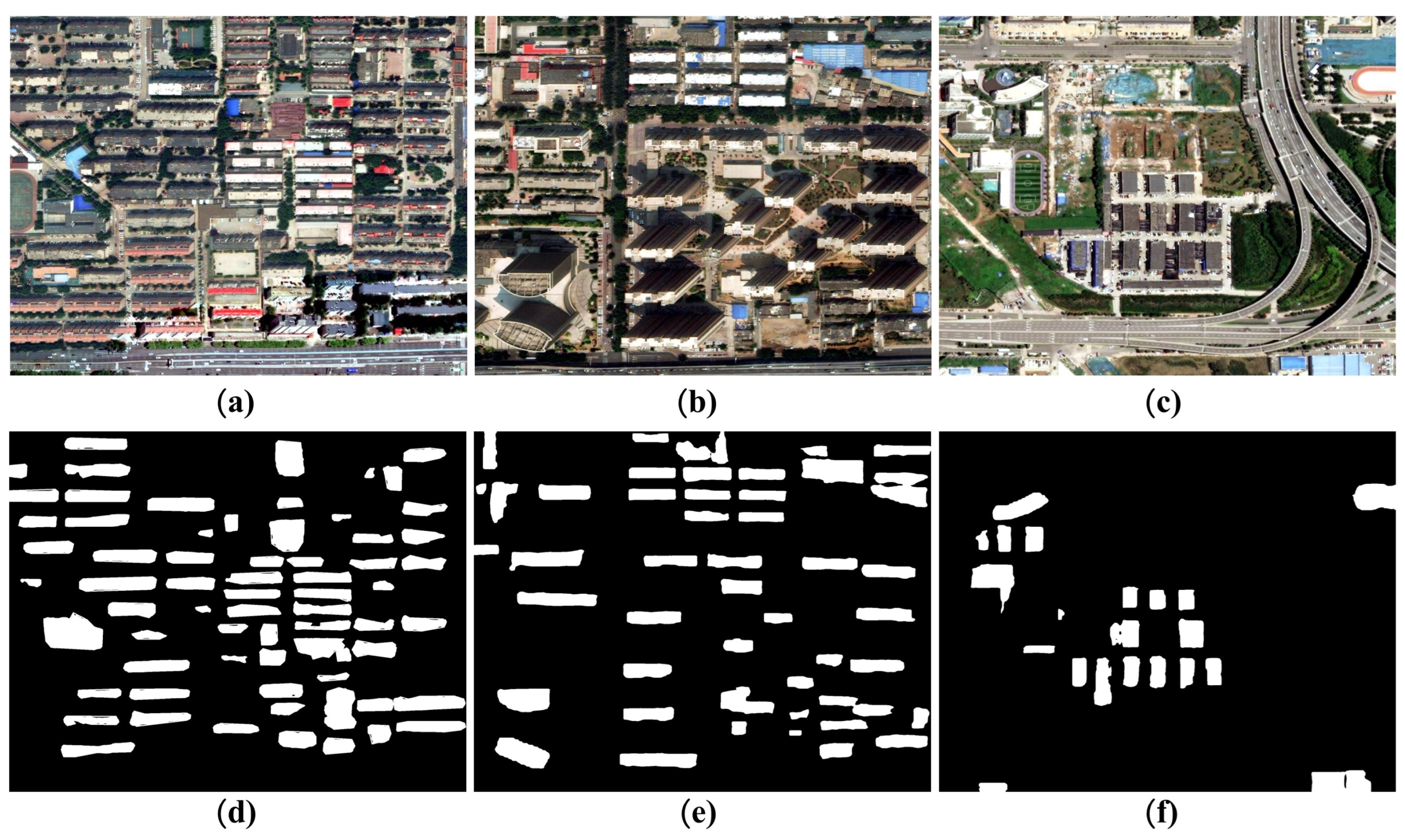
4.1. Instance Segmentation Dataset

Considering that images acquired during UAV flights exhibit a very high spatial resolution, we used Google Earth images with a spatial resolution of 0.3 m as the building instance segmentation dataset, and the sources included the publicly available BONAI dataset [37] and the self-constructed dataset for the Shijiazhuang area in China. The BONAI dataset contains 3300 images of 1024 pixels by 1024 pixels from six cities in China: Shanghai, Beijing, Harbin, Jinan, Chengdu, and Xi’an. As a supplement, 565 image samples from the Shijiazhuang area were used. The roofs of the buildings in all the images are labeled in detail and stored in Common Objects in Context (COCO) format (a commonly used sample set format proposed by Microsoft). A total of 3000 samples were randomly selected as the training set, 450 samples were selected as the validation set, and 415 samples were selected as the test set. Figure 3 shows examples of our dataset.

4.2. Geolocalization Dataset

Although the spatial resolution of low altitude UAV images is usually at the centimeter level, image matching methods typically expect similar or identical resolutions between UAV images and geo-referenced images to ensure matching accuracy. Even though the spatial resolution of UAV images is particularly high, the SOLOv2 algorithm cannot guarantee accurate extraction of the outline of the building. In addition, a high spatial resolution also means a large computational volume and low computational efficiency. Therefore, considering the restrictions of UAV flights inside cities, we referred to the method of Nassar [10] to simulate UAV images of about 0.3 m resolution with Google Earth images. We selected Shijiazhuang, China, as the experimental area. We randomly plotted two routes in Google Earth. The first one occurs in the downtown area with an extremely high building density, and the second one occurs in the suburb area with a relatively low building density. A total of 17 points along the first route and 10 points along the second route were then randomly chosen as UAV image acquisition points. Images with a side length of 500 m, a spatial resolution of 0.235 m along the longitudinal direction, and a spatial resolution of 0.3 m along the latitudinal direction centered on these acquisition points were collected via Google Earth. These images exhibited a resolution of 2127 pixels by 1675 pixels. The latitude and longitude of the image acquisition points were recorded as the ground truth.

4.3. E-Map Dataset

The building outline vector data of Shijiazhuang, as shown in Figure 4, were obtained from Gaode Map (an electronic map navigation software of China). The vector data are based on the GCJ-02 coordinate system, which is a coordinate system obtained by offsetting the WGS84 coordinates. Therefore, the vector data were reprojected to the WGS84 geographic coordinate system via the open-source GIS software Geographic Resources Analysis Support System (GRASS 7.0.3). Moreover, GRASS was used to calculate geometric features, such as the area, aspect ratio, and orientation of the smallest bounding rectangle and the central latitude and longitude of each building. The vector data employed in this study covered an area of over 786 km² in the Shijiazhuang area, with a total data volume of 21.1 Mb.

4.4. Comparison Experiments

The geo-referenced image used in the comparison experiments was a 1 m spatial resolution digital orthophoto image with geographic coordinate information. Notably, the image was refined by the surveying and mapping department. The image acquisition time was 2019, indicating that there were obvious color, imaging perspective, and scale differences between the geo-referenced image and the UAV images, as shown in Figure 5. Assuming that the UAV localization uncertainty is 500 m, an area of 1500 m × 1500 m completely covering the UAV image was randomly cropped within the geo-referenced image as the image patch to be matched. The digital orthophoto image used in the comparison experiments covered an area of 200 km², with a total data volume of 572 Mb.

The RIFT feature matching algorithm is insensitive to nonlinear radiation distortions and has been validated for different types of multimodal image datasets, including optical–optical, infrared–optical and synthetic aperture radar (SAR)–optical datasets [13]. The CFOG method also exhibits better adaptability to image color differences and has been demonstrated as a better algorithm than the MI and HOPC methods [14,21]. Thus, we chose the RIFT and CFOG algorithms as comparison algorithms for the image-based method. Moreover, we chose the SSM map-based method [10] as the ablation comparison algorithm for the SSRM method.

In the RIFT algorithm, both corner and edge points in the PC map are extracted as feature points. Because the PC map is sensitive to the spatial resolution, we resampled the UAV image to the spatial resolution of the geo-referenced image. The log-Gabor convolution sequence was subsequently used to construct the MIM, and the MIM was used to describe feature points via a SIFT-like method. Finally, an exhaustive search method was employed to match the feature points, and the random sample consensus (RANSAC) algorithm was used to filter outliers [13].

The CFOG algorithm was originally used for matching remote sensing images, so it defaults to the presence of geographic projections and coordinates in the images, and the geometric error is relatively small. However, in our experiments, the UAV position uncertainty is 500 m, so we first resampled the UAV image to the spatial resolution of the geo-referenced image and then manually selected eight control point pairs to approximate the transformation relationship between the UAV and geo-referenced images. Afterward, 200 template windows of 140 × 140 pixels in the UAV image were selected to match the geo-referenced image, and the central pixels of the matched windows were regarded as the final matched points [14].

In the SSM algorithm, the geo-reference map is extracted from the e-map with a coverage area of 750 m × 750 m centered on the UAV position. The features of the buildings in the UAV images were matched with those in the geo-reference map one by one. The buildings with the highest sum of the area similarity, minimum bounding rectangle similarity, and orientation similarity were regarded as successfully matched buildings, and duplicate matching pairs were removed [10].

5. Results

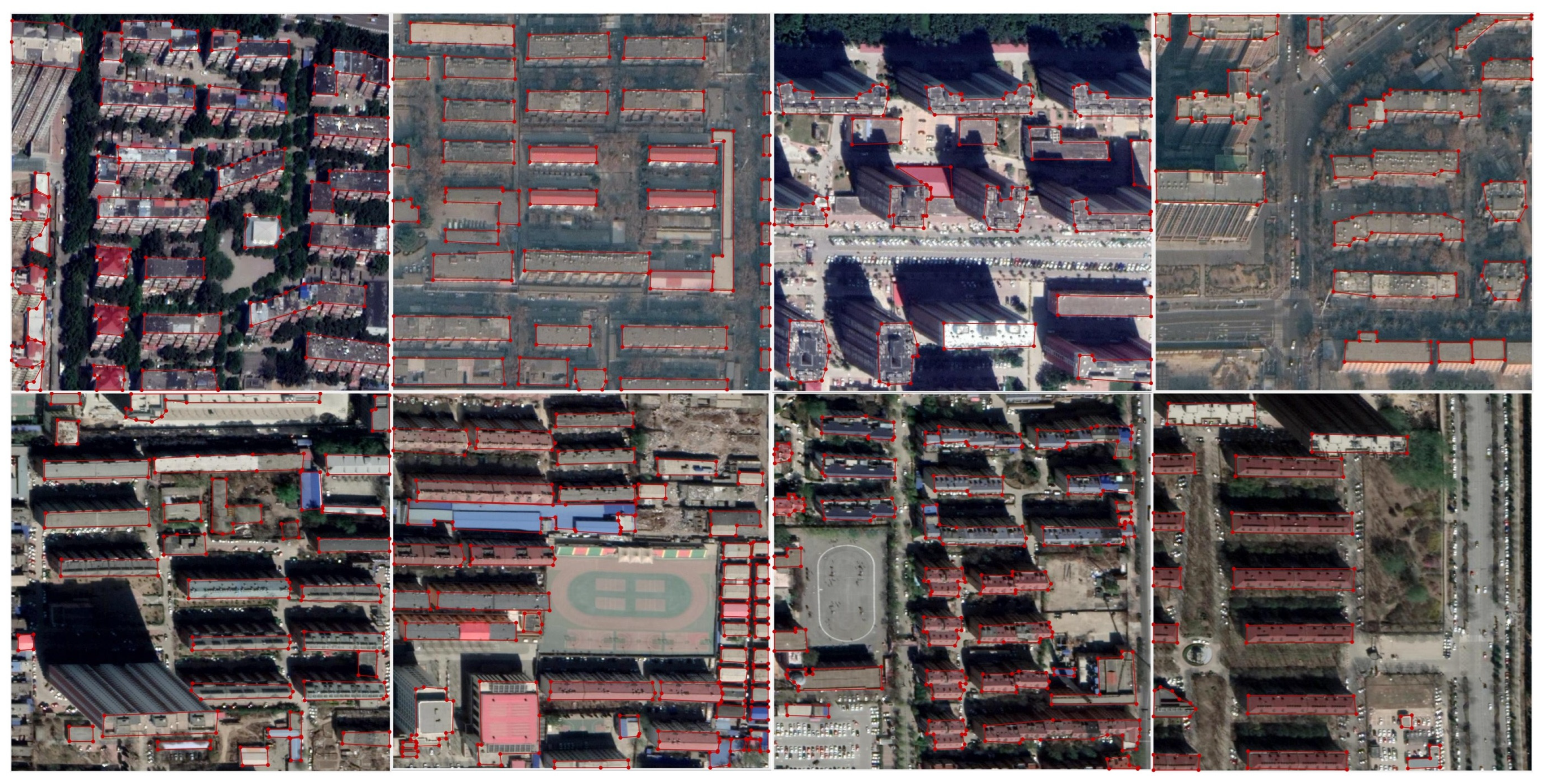
5.1. Instance Segmentation Results

We conducted instance segmentation experiments on a PC with an NVIDIA Tesla V100 GPU and 32 GB of video RAM. Figure 6 shows the building extraction results for some of the UAV images. Buildings with clear outlines and larger areas were extracted well. SOLOv2 achieved a value of 67.4% for AP50, which is the average precision at an intersection over union (IoU) threshold of 0.5, and a value of 64.1% for the recall rate for the test set, which is relatively satisfactory. However, there were still a few cases where buildings with high similarity with the background, small areas, or no obvious differences between individuals (e.g., buildings in urban villages) were missed. Moreover, the outlines of some buildings were not very accurate.

In terms of the processing efficiency, the average processing time for a single UAV image was 0.433 s, with an image interpretation time of 0.4 s and a thinning time of 0.033 s for converting building patches into outline information. Rapid extraction of individual buildings is highly beneficial for real-time UAV localization.

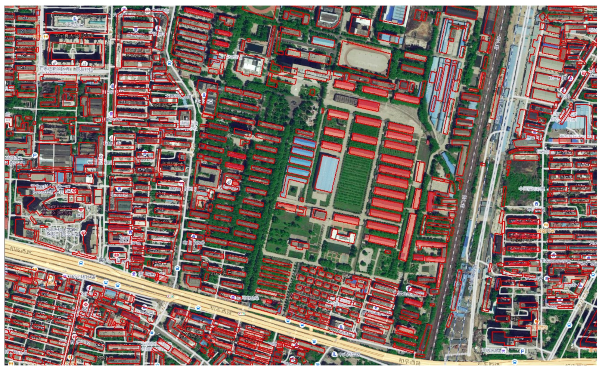
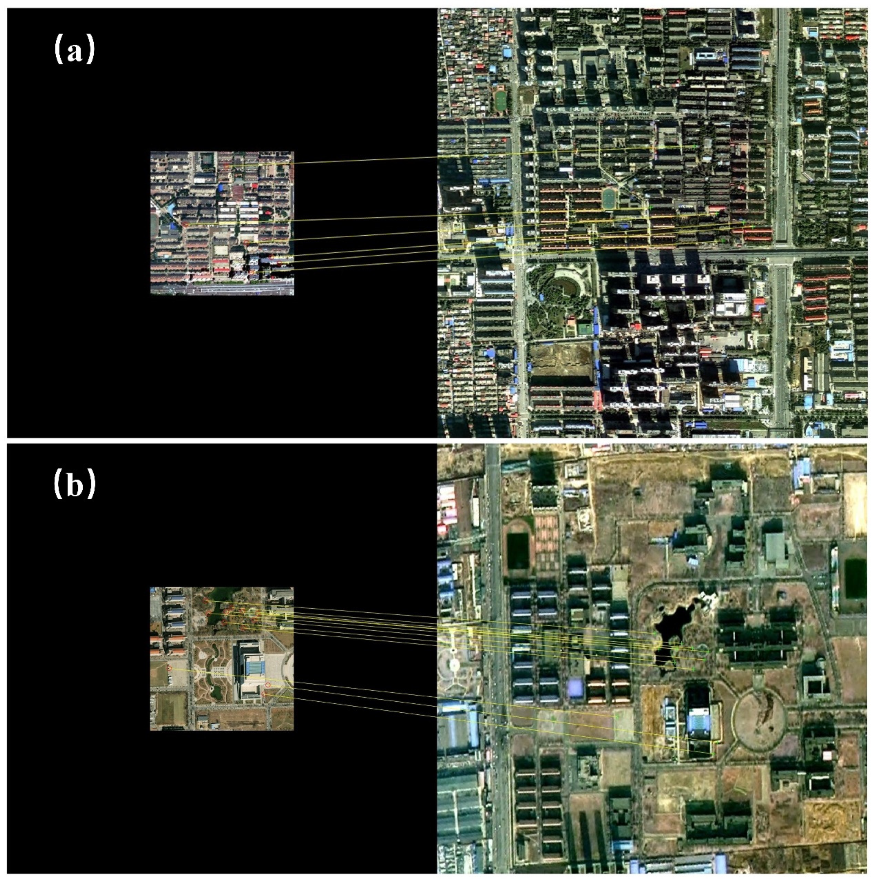
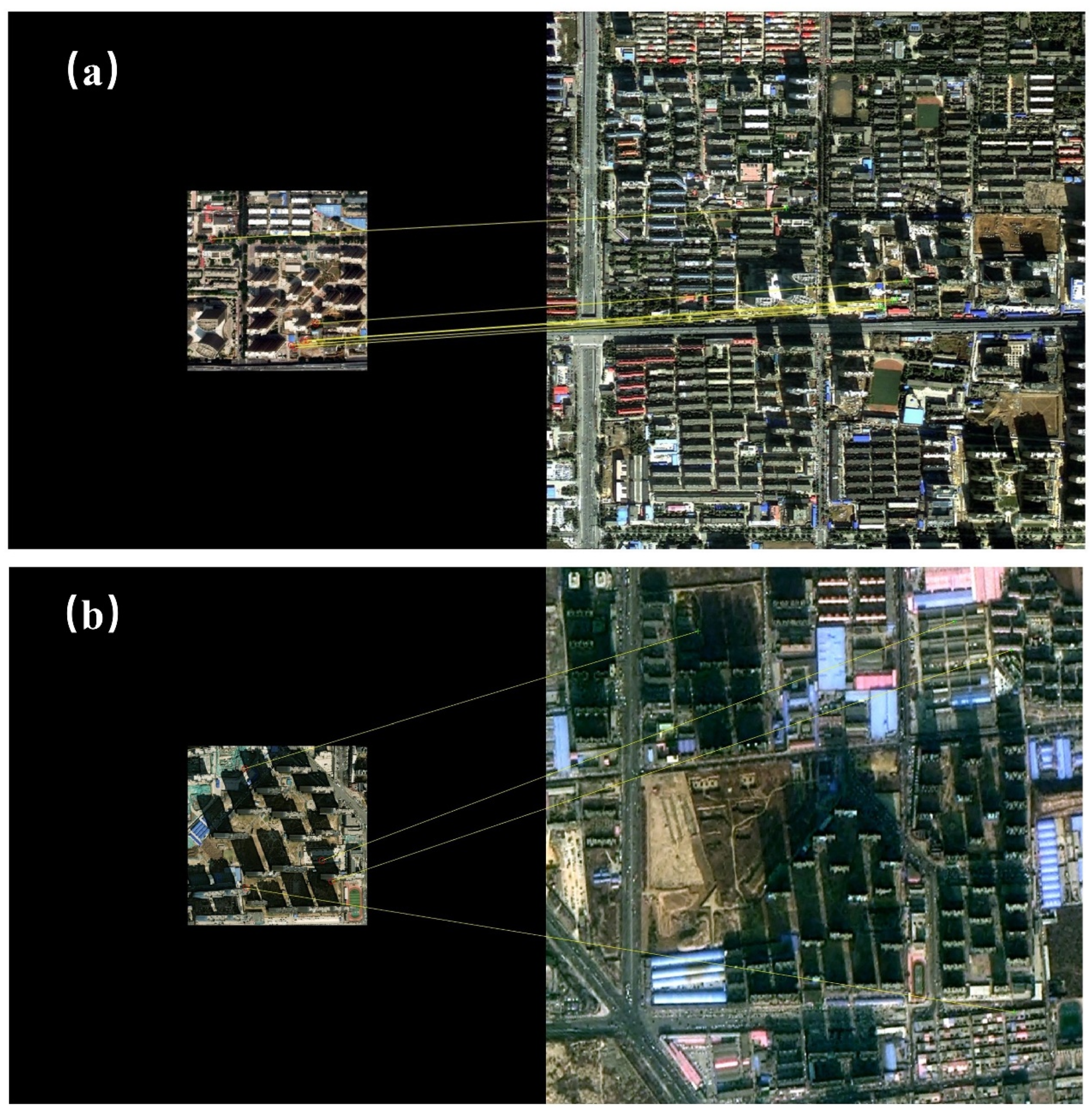
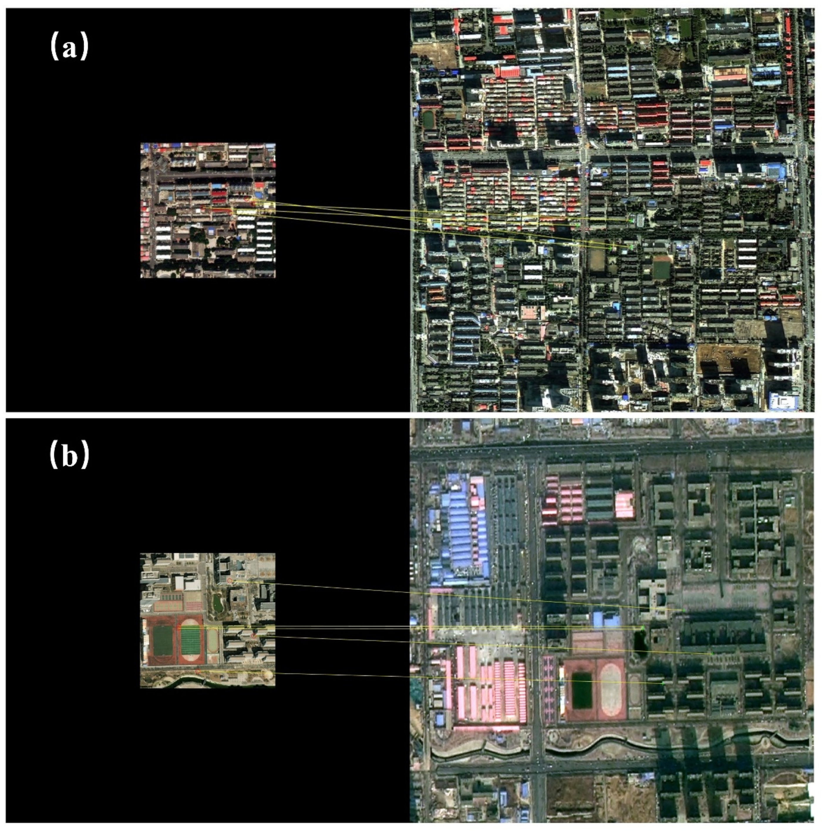
5.2. Scene Matching Results

The matching results of the RIFT algorithm are shown in Figure 7 and Figure 8. Figure 7 shows the results with small matching errors. According to the matching results, although there were differences in the lighting and imaging angles between the UAV and geo-referenced images, the phases between the images remained consistent, so the matching effect was relatively satisfactory. Figure 8 shows the results with a poor match performance. Owing to the existence of high-rise buildings, the significant differences in lighting angles and imaging perspectives resulted in the phase deviating between the UAV and geo-referenced images, leading to a poor matching performance. Therefore, the RIFT algorithm is still greatly influenced by the scene.

Figure 9 shows the matching results of the CFOG algorithm, and almost no feature points were matched correctly. This occurred because the assumption of phase consistency no longer holds when there are obvious lighting angle and imaging perspective differences between the UAV and geo-referenced images.

Figure 10 shows the matching results of the SSM method. Owing to the large number of similar buildings, many individual buildings were mismatched.

Figure 11 shows the matching results of the SSRM method for three scenes. A comparison of Figure 11a–c revealed that although some buildings in the UAV images were missed or demonstrated less accurate edges, the scene matching process filtered out those buildings and successfully matched those with good extraction results and clear contours. A comparison of Figure 11d–f revealed that, owing to sensor side-view imaging, the tops and bottoms of some tall buildings did not completely overlap, so the tops of buildings at different heights did not fully reflect the true spatial relationships among them. However, the scene matching process could facilitate the elimination of this inconsistency, and only buildings with consistent spatial relationships were matched with the e-map. According to the comparison of Figure 11g–i, owing to the phase difference, there were also inconsistencies in the e-map compared with the UAV images, such as redundant buildings, but the scene matching process was resistant to these e-map inaccuracies and could achieve correct scene matching.

5.3. UAV Localization Results

The overall localization performance of each algorithm is detailed in

Table 1. UAV localization results.

Method	Error/m		RMSE/m		Time/s
	Downtown	Suburb	Downtown	Suburb
RIFT	38.46	250.11	105.82	196.77	18.65
CFOG	49.59	59.85	21.45	35.08	2.01
SSM	43.74	96.44	18.12	35.81	0.748
SSRM	7.38	11.92	4.12	7.57	3.58

. The average UAV localization errors of the RIFT algorithm were 38.46 and 250.11 m, with root mean square error (RMSE) values of 105.82 and 196.77 m, for the downtown and suburb datasets, respectively. The average UAV localization errors of the CFOG algorithm were 49.59 and 59.85 m, with RMSE values of 21.45 and 35.08 m, for the downtown and suburb datasets, respectively. The localization results are shown in Figure 12 and Figure 13, and the performance differences among UAV images of different methods are shown in Figure 14. According to Figure 7 and Figure 8, and Table 1, although the RIFT algorithm performed well in matching certain images, its average localization error was still relatively large, indicating that it does not completely overcome the matching difficulties caused by lighting and imaging perspective differences. In addition, the localization error of the RIFT algorithm for the downtown dataset was much smaller than that for the suburb dataset. This occurred because in the suburb dataset, there were significant changes in the land cover type, as well as significant lighting angle and brightness differences between some UAV and geo-referenced images, resulting in significant phase consistency differences between these images and leading to poor matching results. Moreover, the RMSE of the RIFT algorithm was relatively large, indicating that this algorithm is not robust enough and is greatly affected by image scenes. Although the CFOG algorithm could rarely match the feature points correctly, the manually selected control points limited the scope of the template matching process. Therefore, although the average localization accuracy of the CFOG algorithm was low, the localization error and RMSE did not differ much between the urban and suburb datasets.

The SSM method achieved localization errors of 43.74 and 96.44 m, with RMSEs of 18.12 and 35.81 m, for the downtown and suburb datasets, respectively (Figure 12 and Figure 13, respectively). Sparse buildings resulted in poorer performance for the SSM algorithm for the suburb dataset. The shape and orientation features of buildings constrained the range of feature matching. However, multiple similar buildings in the urban scenes still limited the matching accuracy.

The SSRM method achieved average localization errors of 7.38 and 11.92 m, with RMSEs of 1.12 and 7.57 m, for the downtown and suburb datasets, respectively, as shown in Figure 12 and Figure 13, respectively. This demonstrated that the SSRM method significantly reduced the localization error compared with the SSM method, and the denser the buildings are, the higher the localization accuracy. In addition, the SSRM method is robust enough for the different scenes. The SSRM method completely avoids the matching problems caused by land cover change, image illumination, and imaging perspective differences between the UAV and geo-referenced images.

The CFOG algorithm is characterized by high computational efficiency, and its average matching time is 2.01 s. Owing to the complexity of feature point extraction and description, the RIFT algorithm achieves high computational complexity, and its average matching time is 18.65 s (including UAV image resampling). The average time of the SSM algorithm is 0.748 s, with the extraction of buildings from the UAV images requiring 0.4 s and the matching process lasting 0.3 s. The average time of the SSRM method is 3.58 s, of which the average time for building extraction from the UAV images is 0.40 s, the thinning operation time is 0.03 s, and the average time for scene matching based on SSRM is 3.15 s. The computational efficiency of the SSRM method is lower than that of the CFOG and SSM algorithms but significantly greater than that of the RIFT algorithm.

6. Discussion

The building layer of the Gaode map originates from the surveying department and exhibits a small geometric error. Although some buildings in the map may not be consistent with the UAV images due to rapid urban renewal, it does not affect the scene matching process and does not result in UAV localization errors.

The factor that influences the accuracy of the SSRM method is the accuracy of the control points, i.e., the accuracy of the central position of the successfully matched building. The central position of the building outlines is determined by the building extraction process. The deep learning-based building extraction method mainly leads to omission and commission errors and inaccurate outlines. Some buildings with similar features relative to the surrounding background, such as roads, could be missed. The omission of a building will result in it not being used as a ground control point, which does not affect the UAV localization accuracy when there are sufficient control points. Ground targets with similar features to those of buildings may be detected incorrectly. Misdetected buildings exhibit fewer matches in the scene matching process and are not regarded as control points. Thus, they do not affect the UAV localization accuracy.

The building outlines in the e-map represent the bottoms of the buildings, whereas the building outlines extracted from the UAV images represent the building roofs. Because there is an imaging angle in the UAV images, the roof outlines of the buildings do not coincide with the bottom outlines, as shown in Figure 6b, which leads to errors in the control points. For a fixed imaging angle, the higher the building is, the greater the position deviation between the top and bottom outlines in the UAV images and the larger the control point error. When the top outline does not overlap the bottom outline completely, the building is not considered to calculate the control points.

7. Conclusions

In this article, a novel UAV autonomous visual localization method, namely, the SSRM method, is proposed for urban scenes as an alternative to traditional methods based on image matching. The SSRM method first extracts individual buildings from the UAV images, and then uses the shape and spatial relationships of the buildings to match the UAV images with the vector e-map. According to the matching results, control points are generated using the center of the matched buildings, and they are applied to determine the UAV position. The SSRM method can address the impact of lighting, scale, and imaging perspective differences in the image matching process. The SSRM algorithm achieves a smaller localization error in areas with denser buildings. Moreover, the SSRM method requires much less data to be prestored on UAVs than does the image matching method, which is more advantageous in large-area scenarios.

To illustrate the effectiveness of the SSRM method, we apply it to simulated UAV images from Google Earth. In addition, the RIFT, CFOG, and SSM algorithms are utilized for absolute visual localization of UAVs in comparison experiments. The results show that the SSRM method better realizes scene localization and UAV position determination. The obvious difference in performance between the downtown and suburb datasets shows that the RIFT algorithm is not robust enough and is greatly affected by image scenes. The RIFT algorithm may still fail when there are obvious land cover changes or lighting angle and brightness differences between the UAV and geo-referenced images, because the assumption of phase consistency may not hold. The CFOG algorithm still cannot overcome the problems caused by lighting and imaging differences. The SSM algorithm, although extremely efficient computationally, results in incorrect matching due to the high similarity of buildings, further yielding a low localization performance. The results show that the SSRM method achieves better localization accuracy and is more robust.

Considering that the shape and spatial relationships of buildings are used for scene matching in the SSRM method, it may fail when dense buildings do not occur in UAV images for a long period. In addition, the SSRM method requires known orientation and scale information of the UAV images, and a possible future research direction is a scene matching method given an unknown orientation and scale of the UAV images.

References

1. Couturier, A.; Akhloufi, M.A. A review on absolute visual localization for UAV. Robot. Auton. Syst. 2021, 135, 103666. [Google Scholar]
2. Kinnari, J.; Verdoja, F.; Kyrki, V. GNSS-Denied Geolocalization of UAVs by Visual Matching of Onboard Camera Images with Orthophotos. In Proceedings of the 20th International Conference on Advanced Robotics, ICAR 2021, Manhattan, NY, USA, 6–10 December 2021; pp. 555–562. [Google Scholar]
3. Gui, J.; Gu, D.; Wang, S.; Hu, H. A review of visual inertial odometry from filtering and optimisation perspectives. Adv. Robot. 2015, 29, 1289–1301. [Google Scholar]
4. Liu, Y.; Bai, J.; Wang, G.; Wu, X.; Sun, F.; Guo, Z.; Geng, H. UAV Localization in Low-Altitude GNSS-Denied Environments Based on POI and Store Signage Text Matching in UAV Images. Drones 2023, 7, 451. [Google Scholar] [CrossRef]
5. Li, W. Research on UAV Localization Method based on Image Registration and System Design. Master Degree, Univeristy of Electronic Science and Technology, Chengdu, China, 2023. [Google Scholar]
6. Boiteau, S.; Vanegas, F.; Gonzalez, F. Framework for Autonomous UAV Navigation and Target Detection in Global-Navigation-Satellite-System-Denied and Visually Degraded Environments. Remote Sens. 2024, 16, 471. [Google Scholar] [CrossRef]
7. Zhao, C.; Zhou, Y.; Lin, Z.; Hu, J.; Pan, Q. Review of scene matching visual navigation for unmanned aerial vehicles. Sci. Sin. Inf. 2019, 49, 507–519. [Google Scholar]
8. Chen, J.; Chen, C.; Chen, Y. Fast algorithm for robust template matching with M-estimators. IEEE Trans. Signal Process. 2003, 51, 230–243. [Google Scholar]
9. Xu, Y.; Pan, L.; Du, C.; Li, J.; Jing, N.; Wu, J. Vision-based UAVs Aerial Image Localization: A Survey. In Proceedings of the 2nd ACM SIGSPATIAL International Workshop on AI for Geographic Knowledge Discovery, Seattle, WA, USA, 6 November 2018; pp. 8–18. [Google Scholar]
10. Nassar, A.; Amer, K.; ElHakim, R.; ElHelw, M. A Deep CNN-Based Framework For Enhanced Aerial Imagery Registration with Applications to UAV Geolocalization. In Proceedings of the IEEE/CVF Conference on Computer Vision and Pattern Recognition Workshops, Salt Lake City, UT, USA, 18–23 June 2018; pp. 1594–1604. [Google Scholar]
11. Choi, J.; Myung, H. BRM Localization: UAV localization in GNSS-denied environments based on matching of numerical map and UAV images. In Proceedings of the 2020 IEEE/RSJ International Conference on Intelligent Robots and Systems (IROS), Las Vegas, NV, USA, 25–29 October 2020; pp. 4537–4544. [Google Scholar]
12. Buck, A.R.; Keller, J.M.; Skubic, M. A modified genetic algorithm for matching building sets with the histograms of forces. In Proceedings of the IEEE Congress on Evolutionary Computation, Brisbane, Australia, 10–15 June 2012; pp. 1–7. [Google Scholar]
13. Li, J.; Hu, Q.; Ai, M. RIFT: Multi-Modal Image Matching Based on Radiation-Variation Insensitive Feature Transform. IEEE Trans. Image Process. 2020, 29, 3296–3310. [Google Scholar]
14. Ye, Y.; Bruzzone, L.; Shan, J.; Bovolo, F.; Zhu, Q. Fast and Robust Matching for Multimodal Remote Sensing Image Registration. IEEE Trans. Geosci. Remote 2019, 57, 9059–9070. [Google Scholar]
15. Zhang, X.; Leng, C.; Hong, Y.; Pei, Z.; Cheng, I.; Basu, A. Multimodal Remote Sensing Image Registration Methods and Advancements: A Survey. Remote Sens. 2021, 13, 5128. [Google Scholar] [CrossRef]
16. Lewis, J.P. Fast Template Matching. In Vision Interface 95; Canadian Image Processing and Pattern Recognition Society, Quebec, Canada, 15–19 May 1995; Canadian Image Processing and Pattern Recognition Society: Toronto, ON, Canada; Volume 95, pp. 120–123.
17. Wan, X.; Liu, J.; Yan, H.; Morgan, G.L.K. Illumination-invariant image matching for autonomous UAV localisation based on optical sensing. ISPRS J. Photogramm. Remote Sens. 2016, 119, 198–213. [Google Scholar]
18. Patel, B.; Barfoot, T.D.; Schoellig, A.P. Visual Localization with Google Earth Images for Robust Global Pose Estimation of UAVs. In Proceedings of the IEEE International Conference on Robotics and Automation (ICRA), Paris, France, 31 May–31 August 2020; pp. 6491–6497. [Google Scholar]
19. Sibiryakov, A. Fast and high-performance template matching method. In Proceedings of the IEEE Conference on Computer Vision and Pattern Recognition, Colorado Springs, CO, USA, 20–25 June 2011; pp. 1417–1424. [Google Scholar]
20. Ye, Y.; Shan, J.; Hao, S.; Bruzzone, L.; Qin, Y. A local phase based invariant feature for remote sensing image matching. ISPRS J. Photogramm. Remote Sens. 2018, 142, 205–221. [Google Scholar]
21. Fan, Z.; Zhang, L.; Liu, Y.; Wang, Q.; Zlatanova, S. Exploiting High Geopositioning Accuracy of SAR Data to Obtain Accurate Geometric Orientation of Optical Satellite Images. Remote Sens. 2021, 13, 3535. [Google Scholar] [CrossRef]
22. Haigang, S.; Chang, L.; Zhe, G.; Zhengjie, J.; Chuan, X. Overview of multi-modal remote sensing image matching methods. Acta Geod. Cartogr. Sin. 2022, 51, 1848–1861. [Google Scholar]
23. Mantelli, M.; Pittol, D.; Neuland, R.; Ribacki, A.; Maffei, R.; Jorge, V.; Prestes, E.; Kolberg, M. A novel measurement model based on abBRIEF for global localization of a UAV over satellite images. Robot. Auton. Syst. 2019, 112, 304–319. [Google Scholar]
24. Dusmanu, M.; Rocco, I.; Pajdla, T.; Pollefeys, M.; Sivic, J.; Torii, A.; Sattler, T. D2-Net: A Trainable CNN for Joint Detection and Description of Local Features. In Proceedings of the 2019 IEEE/CVF Conference on Computer Vision and Pattern Recognition (CVPR), Long Beach, CA, USA, 15–20 June 2019; pp. 8084–8093. [Google Scholar]
25. Kumar, B.V.; Carneiro, G.; Reid, I. Learning local image descriptors with deep siamese and triplet convolutional networks by minimising global loss functions. In Proceedings of the 2016 IEEE Conference on Computer Vision and Pattern Recognition (CVPR), Las Vegas, NV, USA, 26 June–1 July 2016; pp. 5385–5394. [Google Scholar]
26. DeTone, D.; Malisiewicz, T.; Rabinovich, A. SuperPoint: Self-Supervised Interest Point Detection and Description. In Proceedings of the IEEE Conference on Computer Vision and Pattern Recognition Workshops, Salt Lake City, UT, USA, 18–22 June 2018; pp. 224–236. [Google Scholar]
27. Sarlin, P.; DeTone, D.; Malisiewicz, T.; Rabinovich, A. SuperGlue: Learning Feature Matching with Graph Neural Networks. In Proceedings of the 2020 IEEE/CVF Conference on Computer Vision and Pattern Recognition (CVPR), Seattle, WA, USA, 14–19 June 2020; pp. 4937–4946. [Google Scholar]
28. Sun, J.; Shen, Z.; Wang, Y.; Bao, H.; Zhou, X. LoFTR: Detector-Free Local Feature Matching with Transformers. In Proceedings of the IEEE/CVF Conference on Computer Vision and Pattern Recognition, Nashville, TN, USA, 19–25 June 2021; pp. 8918–8927. [Google Scholar]
29. Masselli, A.; Hanten, R.; Zell, A. Localization of Unmanned Aerial Vehicles Using Terrain Classification from Aerial Images. Intell. Auton. Syst. 2016, 13, 831–842. [Google Scholar]
30. Yun, H.; Ziyang, M.; Jiawen, A.; Yuanqing, W. Localization method by aerial image matching in urban environment based on semantic segmentation. J. Huazhong Univerisity Sci. Technol. (Nat. Sci. Ed.) 2022, 11, 79–84. [Google Scholar]
31. Wang, H.; Cheng, Y.; Liu, N.; Zhao, Y.; Chan, H.C. An illumination-invariant shadow-based scene matching navigation approach in low-altitude flight. Remote Sens. 2022, 14, 3869. [Google Scholar] [CrossRef]
32. Shan, M.; Wang, F.; Lin, F.; Gao, Z.; Tang, Y.Z.; Chen, B.M. Google map aided visual navigation for UAVs in GPS-denied environment. In Proceedings of the IEEE Conference on Robotics and Biomimetics, Zhuhai, China, 6–9 December 2015; pp. 114–119. [Google Scholar]
33. Yol, A.; Delabarre, B.; Dame, A.; Dartois, J.; Marchand, E. Vision-based absolute localization for unmanned aerial vehicles. In Proceedings of the IEEE/RSJ International Conference on Intelligent Robots and Systems (IROS), Chicago, IL, USA, 14–18 September 2014; pp. 3429–3434. [Google Scholar]
34. Sun, L.; Sun, Y.; Yuan, S.; Ai, M. A survey of instance segmentation research based on deep learning. CAAI Trans. Intell. Syst. 2022, 17, 16. [Google Scholar]
35. Wang, X.; Zhang, R.; Kong, T.; Li, L.; Shen, C. SOLOv2: Dynamic and Fast Instance Segmentation. Adv. Neural Inf. Process. Syst. 2020, 33, 17721–17732. [Google Scholar]
36. Douglas, D.H.; Peucher, T.K. Algorithms for the reduction of the number of points required to represent a digitized line or its caricature. Int. J. Geogr. Inf. Sci. 1973, 2, 112–122. [Google Scholar]
37. Wang, J.; Meng, L.; Li, W.; Yang, W.; Yu, L.; Xia, G.S. Learning to Extract Building Footprints From Off-Nadir Aerial Images. IEEE Trans. Pattern Anal. Mach. Intell. 2023, 45, 1294–1301. [Google Scholar] [PubMed]
Figure 1. Flowchart of UAV autonomous localization in urban scenarios based on shape and spatial relationship matching of buildings.
Remotesensing 16 03065 g001
Figure 2. Basic diagram of the SSRM method.
Remotesensing 16 03065 g002
Figure 3. Examples of instance segmentation datasets. The red boxes are the labeled outlines of buildings.
Remotesensing 16 03065 g003
Figure 4. Electronic map vector data of a region in Shijiazhuang city from Gaode Map (an electronic map navigation software of China), superimposed on a satellite remote sensing image.
Remotesensing 16 03065 g004
Figure 5. Comparison between the UAV and geo-referenced image in the comparison experiments. (a,c) show UAV images and (b,d) show subsets of the geo-referenced image, and the red boxes indicate the positions of the UAV images in the subset.
Remotesensing 16 03065 g005
Figure 6. Building extraction results. (ac) show UAV images and (df) show building mask maps. (a,b) show the downtown area and (c) shows the suburb area.
Remotesensing 16 03065 g006
Figure 7. Good matching results of the RIFT algorithm. (a) shows the downtown area and (b) shows the suburb area.
Remotesensing 16 03065 g007
Figure 8. Poor matching results of the RIFT algorithm. (a) shows the downtown area and (b) shows the suburb area.
Remotesensing 16 03065 g008
Figure 9. Matching results of the CFOG algorithm. (a) shows the downtown area and (b) shows the suburb area.
Remotesensing 16 03065 g009
Figure 10. Matching results of the SSM method. (a,d) show the UAV images, (b,e) show the building extraction results, and (c,f) show the e-maps. (a) shows the downtown area and (d) shows the suburb area. The red points indicate the central points of the buildings, and the points connected by the green lines indicate the successfully matched buildings.
Remotesensing 16 03065 g010
Figure 11. Scene matching results of the SSRM method. (a,d,g) UAV images; (b,e,h) building extraction results from the UAV images; and (c,f,i) e-map data. (a,d) Downtown area and (g) suburb area. The red points indicate the central points of the buildings, and the points connected by the green lines indicate the successfully matched buildings.
Remotesensing 16 03065 g011
Figure 12. UAV localization results for the downtown dataset. The black line indicates the real UAV flight path, and the red, green, blue, and purple lines indicate the UAV flight paths estimated by SSRM, RIFT, CFOG, and SSM methods, respectively.
Remotesensing 16 03065 g012
Figure 13. UAV localization results for the suburb dataset. The black line indicates the real UAV flight path, and the red, green, blue, and purple lines indicate the UAV flight paths estimated by the SSRM, RIFT, CFOG, and SSM methods, respectively.
Remotesensing 16 03065 g013
Figure 14. Comparison of the UAV localization errors of the different algorithms.
Remotesensing 16 03065 g014