
Sensitivity of Local Climate Zones and Urban Functional Zones to Multi-Scenario Surface Urban Heat Islands


Abstract
1. Introduction
2. Study Area and Data
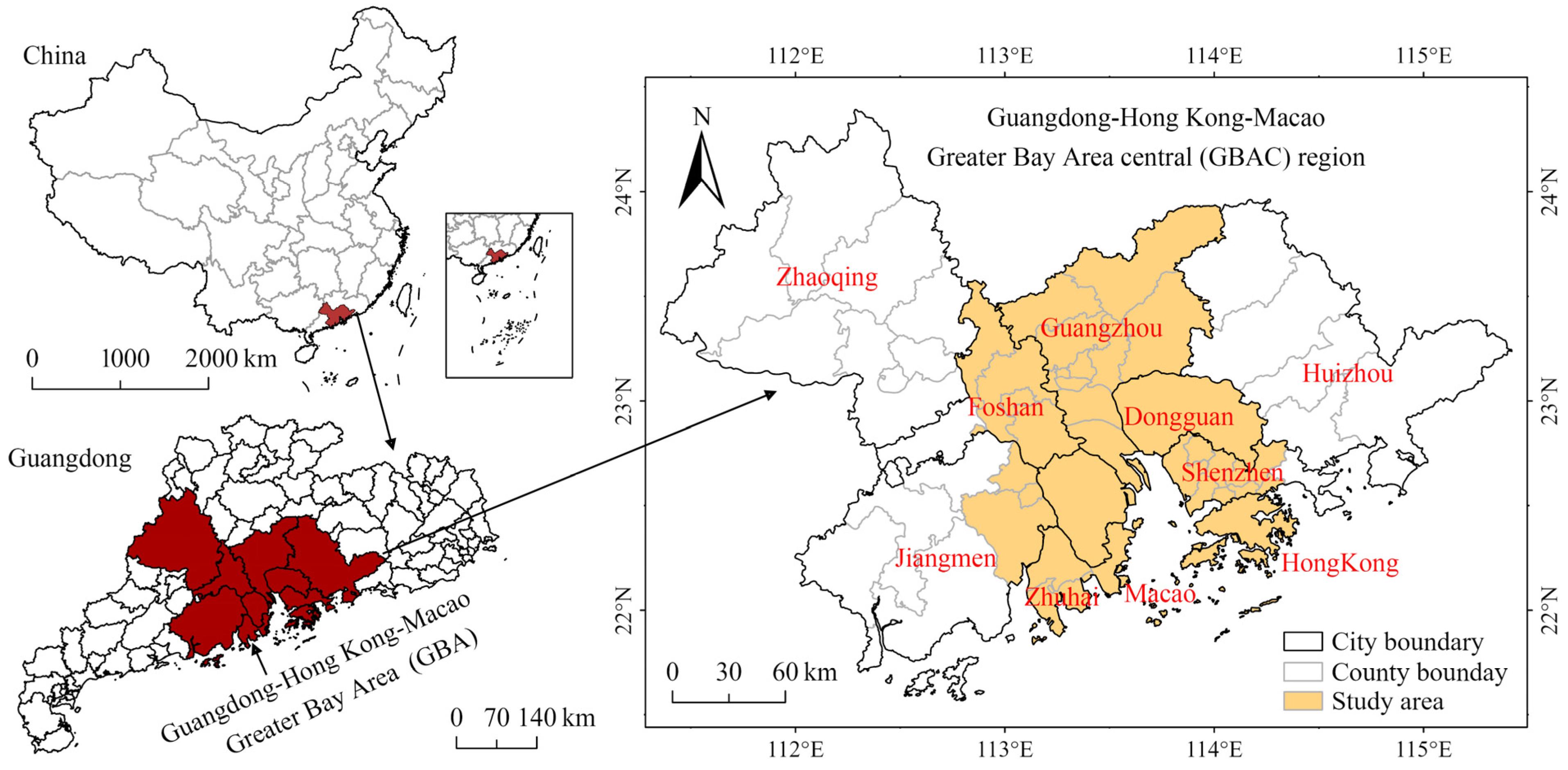
2.1. Study Area
2.2. Data Source and Processing

| Type | Spatial Resolution | Date | Sources |
|---|---|---|---|
| Landsat 8 image | 0.03 km | 14 November 2019 | Chinese Academy of Sciences Geospatial Data Cloud |
| MODIS image | 1 km | 11 November 2019 to 17 November 2019 | GEE (https://doi.org/10.5067/MODIS/MOD11A1.061, accessed on 26 January 2024) |
| Meteorological observation data | - | 14 November 2019 | GBAMWF |
| LCZ data | 0.1 km | 2019 | [39] |
| UFZ data | - | 2018 | [40] |
| POI data | - | 2018 | AutoNavi map |
| Road data | - | 2019 | Open Street Map |
| Building data | - | 2018 | Baidu Map |
| Population density data | 0.1 km | 2019 | WorldPop (https://hub.worldpop.org/, accessed on 22 January 2024) |
| Luojia01 nighttime light data | 0.13 km | 2019 | Wuhan University (http://59.175.109.173:8888/app/login.html, accessed on 21 January 2024) |
| Land use/cover data | 0.03 km | 2019 | [38] |
| ASTER GDEM V3 dataset | 0.03 km | 2019 | https://srtm.csi.cgiar.org/, accessed on 13 January 2024 |
| Urban area boundary data | 0.25 km | 2018 | [42] |
| China coastline data | - | 2021 | https://www.webmap.cn/commres.do?method=result100W, accessed on 11 January 2024 |
3. Methodology
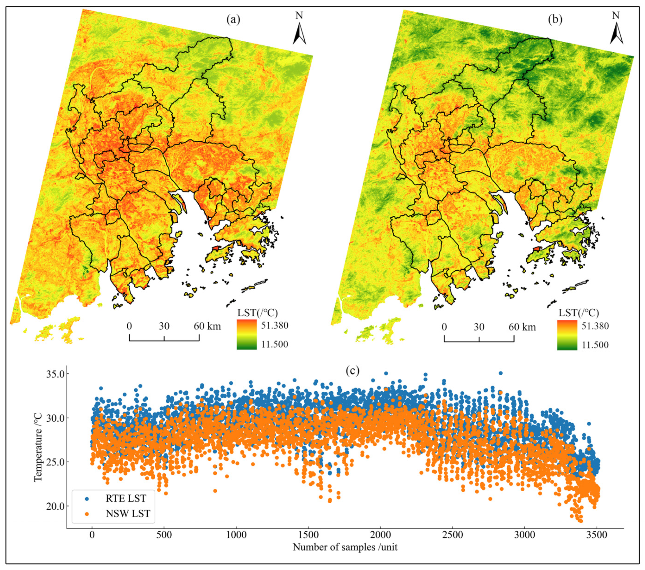
3.1. LST Retrieval
- (1)
- Radiative transfer equation (RTE) method
- (2)
- Nonlinear split-window (NSW) method
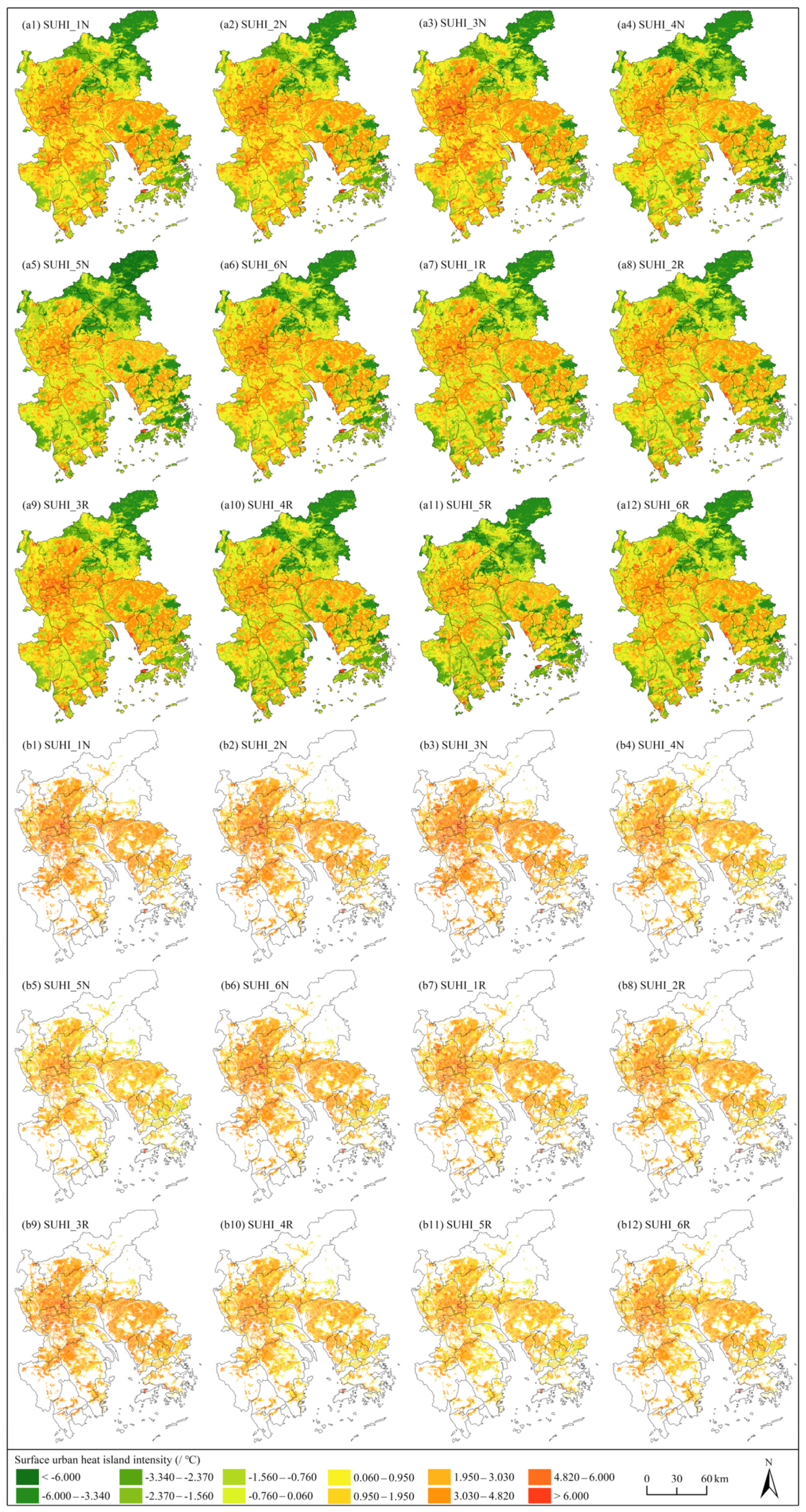
3.2. Calculation of SUHI
3.3. Spatial Gradient Boosting Trees (SGBT)
3.4. Geographically Weighted Regression Model (GWR)
4. Analysis and Results
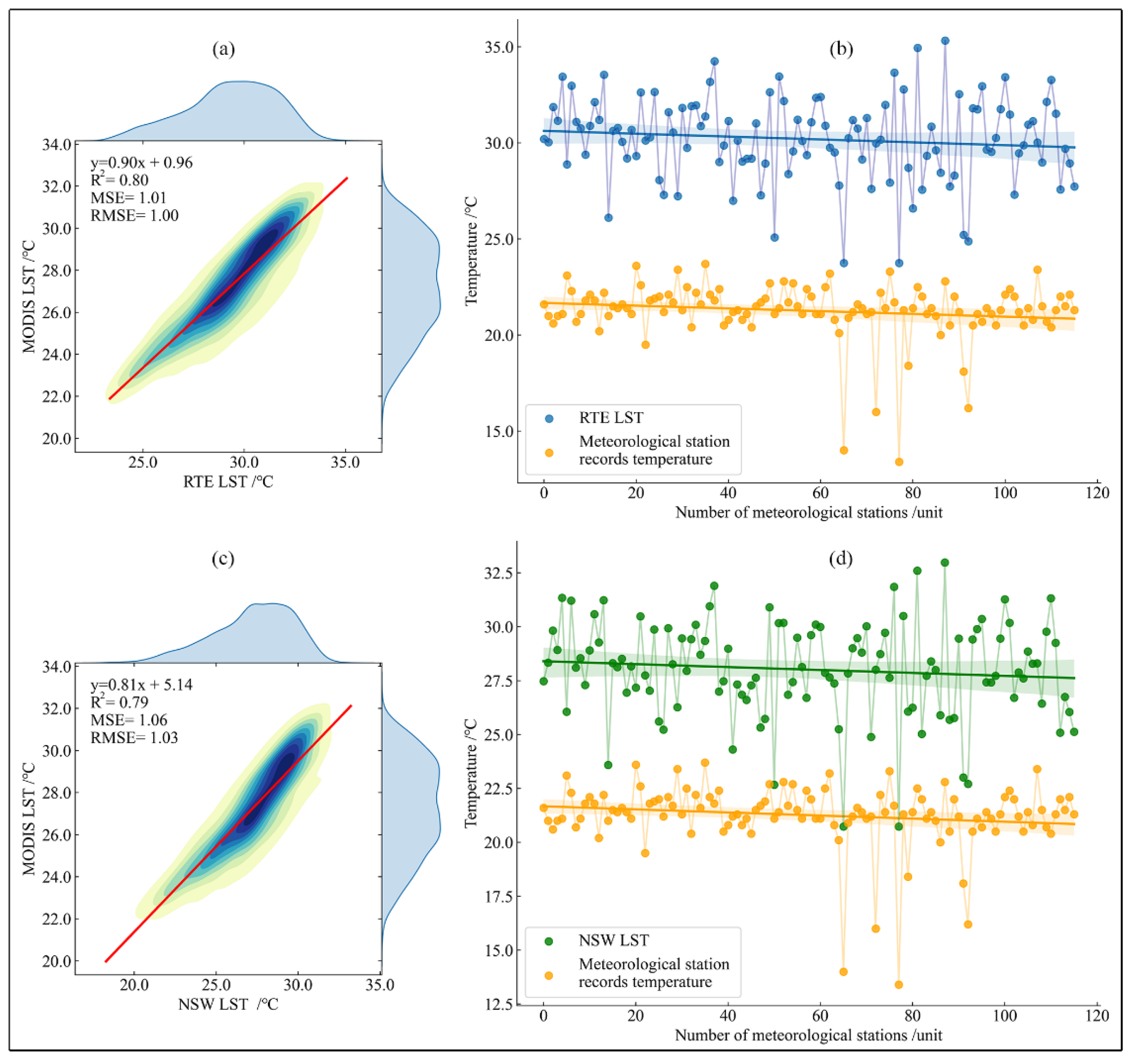
4.1. LST Validation
4.2. Sensitivity Analysis of LCZ Types and UFZ Types on SUHI
4.3. SUHI Influencing Factor Sensitivity
4.3.1. Global Sensitivity of SUHI Influencing Factors
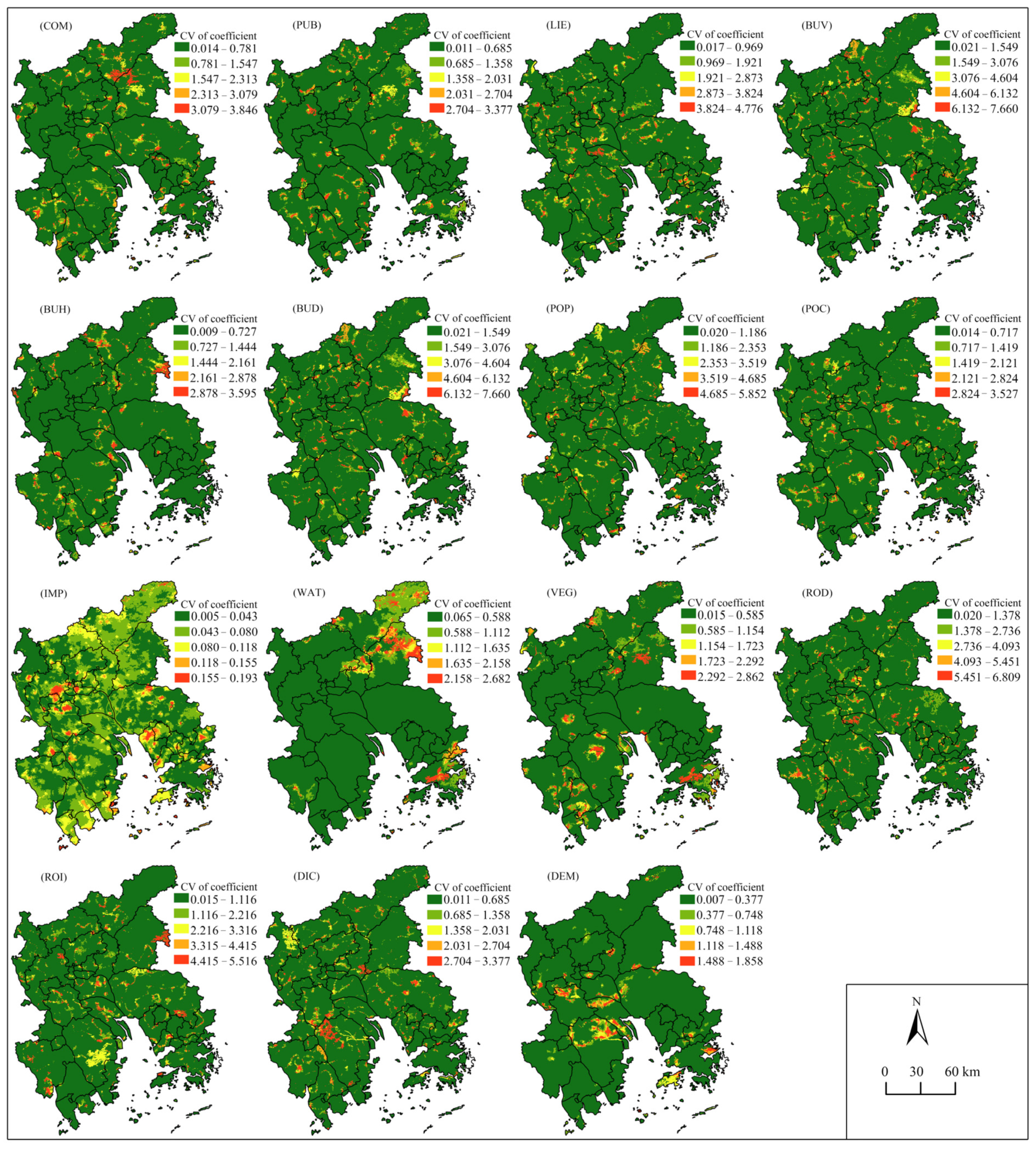
4.3.2. Local Spatial Sensitivity of SUHI Influencing Factors
5. Discussion
5.1. Uncertainty in SUHI Assessment
5.2. The Impact of Zoning Schemes of Analysis Units on SUHI Sensitivity
5.3. Insights and Recommendations for Urban Planning and Management
5.4. Limitations
6. Conclusions
Author Contributions
Funding
Data Availability Statement
Acknowledgments
Conflicts of Interest
Abbreviations
Appendix A
| Type | Count | TArea | Type | Count | TArea |
|---|---|---|---|---|---|
| LCZ 1 | 620 | 182.181 | LCZ A | 3224 | 4649.731 |
| LCZ 2 | 2022 | 566.731 | LCZ B | 3289 | 948.687 |
| LCZ 3 | 2863 | 1075.486 | LCZ C | 1336 | 242.570 |
| LCZ 4 | 3313 | 1051.295 | LCZ D | 5394 | 3421.576 |
| LCZ 5 | 1419 | 363.671 | LCZ E | 354 | 150.147 |
| LCZ 6 | 1742 | 458.427 | LCZ F | 1831 | 713.175 |
| LCZ 7 | 637 | 444.014 | LCZ G | 2637 | 1723.696 |
| LCZ 8 | 2855 | 3044.345 | |||
| LCZ 9 | 4375 | 1082.230 | |||
| LCZ 10 | 400 | 87.114 |
| Level 1 | Level 2 | Descriptions | Count |
|---|---|---|---|
| 01 Residential | 0101 Residential | Houses and apartment buildings-places where people live. | 8612 |
| 02 Commercial | 0201 Business | Buildings where people work, including office buildings, and commercial office places for finance, internet technology, e-commerce, media, etc. | 1364 |
| 0202 Commercial service | Houses and buildings for commercial retails, restaurants, lodging, and entertainment. | 2200 | |
| 03 Industrial | 0301 Industrial | Land and buildings used for manufacturing, warehouse, mining, etc. | 8311 |
| 04 Transportation | 0402 Transportation stations | Transportation facilities including motor, bus, and train stations and ancillary facilities. | 303 |
| 0403 Airport facilities | Airports for civil, military, and mixed uses. | 113 | |
| 05 Public management and service | 0501 Administrative | Lands used for government, military, and public service agencies. | 917 |
| 0502 Educational | Lands used for education and research, including schools, universities, institutes, and their ancillary facilities. | 1826 | |
| 0503 Medical | Lands used for hospitals, disease prevention, and emergency services. | 808 | |
| 0504 Sport and cultural | Lands used for public sports, training, and cultural services, including gym center, libraries, museums, exhibition centers, etc. | 844 | |
| 0505 Park and greenspace | Parks and greenspace lands used for entertainment and environmental conservations. | 3396 | |
| 06 Mixed-Use | 0601 Mixed-use | Integration of diverse functionalities, such as the combination of residential and commercial, commercial and office, etc. | 1724 |
| Factors | SUHI_1N | SUHI_2N | SUHI_3N | SUHI_4N | SUHI_5N | SUHI_6N | SUHI_1R | SUHI_2R | SUHI_3R | SUHI_4R | SUHI_5R | SUHI_6R |
|---|---|---|---|---|---|---|---|---|---|---|---|---|
| Intercept | 26.842 | 26.812 | 27.598 | 25.928 | 25.433 | 26.395 | 25.773 | 25.732 | 26.495 | 25.471 | 25.241 | 25.668 |
| COM | 1.522 | 1.522 | 1.522 | 1.522 | 1.522 | 1.522 | 1.522 | 1.522 | 1.522 | 1.522 | 1.522 | 1.522 |
| PUB | 2.816 | 2.816 | 2.816 | 2.816 | 2.816 | 2.816 | 2.822 | 2.822 | 2.822 | 2.822 | 2.822 | 2.822 |
| LIE | 2.477 | 2.477 | 2.477 | 2.477 | 2.477 | 2.477 | 2.477 | 2.477 | 2.477 | 2.477 | 2.477 | 2.477 |
| BUV | 1.150 | 1.150 | 1.150 | 1.150 | 1.150 | 1.150 | 1.151 | 1.151 | 1.151 | 1.151 | 1.151 | 1.151 |
| BUH | 1.826 | 1.826 | 1.826 | 1.826 | 1.826 | 1.826 | 1.820 | 1.820 | 1.820 | 1.820 | 1.820 | 1.820 |
| BUD | 2.223 | 2.223 | 2.223 | 2.223 | 2.223 | 2.223 | 2.218 | 2.218 | 2.218 | 2.218 | 2.218 | 2.218 |
| POP | 1.649 | 1.649 | 1.649 | 1.649 | 1.649 | 1.649 | 1.649 | 1.649 | 1.649 | 1.649 | 1.649 | 1.649 |
| POC | 1.823 | 1.823 | 1.823 | 1.823 | 1.823 | 1.823 | 1.825 | 1.825 | 1.825 | 1.825 | 1.825 | 1.825 |
| IMP | 3.915 | 3.915 | 3.915 | 3.915 | 3.915 | 3.915 | 3.904 | 3.904 | 3.904 | 3.904 | 3.904 | 3.904 |
| WAT | 1.494 | 1.494 | 1.494 | 1.494 | 1.494 | 1.494 | 1.594 | 1.594 | 1.594 | 1.594 | 1.594 | 1.594 |
| VEG | 2.981 | 2.981 | 2.981 | 2.981 | 2.981 | 2.981 | 2.941 | 2.941 | 2.941 | 2.941 | 2.941 | 2.941 |
| ROD | 2.788 | 2.788 | 2.788 | 2.788 | 2.788 | 2.788 | 2.794 | 2.794 | 2.794 | 2.794 | 2.794 | 2.794 |
| ROI | 1.470 | 1.470 | 1.470 | 1.470 | 1.470 | 1.470 | 1.465 | 1.465 | 1.465 | 1.465 | 1.465 | 1.465 |
| DIC | 1.189 | 1.189 | 1.189 | 1.189 | 1.189 | 1.189 | 1.181 | 1.181 | 1.181 | 1.181 | 1.181 | 1.181 |
| DEM | 1.612 | 1.612 | 1.612 | 1.612 | 1.612 | 1.612 | 1.535 | 1.535 | 1.535 | 1.535 | 1.535 | 1.535 |
| Factors | SUHI_1N | SUHI_2N | SUHI_3N | SUHI_4N | SUHI_5N | SUHI_6N | SUHI_1R | SUHI_2R | SUHI_3R | SUHI_4R | SUHI_5R | SUHI_6R |
|---|---|---|---|---|---|---|---|---|---|---|---|---|
| Intercept | 107.343 | 107.275 | 108.935 | 105.061 | 103.397 | 106.297 | 106.131 | 105.987 | 108.227 | 104.991 | 103.787 | 105.763 |
| COM | 1.509 | 1.509 | 1.509 | 1.509 | 1.509 | 1.509 | 1.510 | 1.510 | 1.510 | 1.510 | 1.510 | 1.510 |
| PUB | 2.088 | 2.088 | 2.088 | 2.088 | 2.088 | 2.088 | 2.089 | 2.089 | 2.089 | 2.089 | 2.089 | 2.089 |
| LIE | 1.751 | 1.751 | 1.751 | 1.751 | 1.751 | 1.751 | 1.751 | 1.751 | 1.751 | 1.751 | 1.751 | 1.751 |
| BUV | 1.153 | 1.153 | 1.153 | 1.153 | 1.153 | 1.153 | 1.158 | 1.158 | 1.158 | 1.158 | 1.158 | 1.158 |
| BUH | 1.826 | 1.826 | 1.826 | 1.826 | 1.826 | 1.826 | 1.846 | 1.846 | 1.846 | 1.846 | 1.846 | 1.846 |
| BUD | 1.679 | 1.679 | 1.679 | 1.679 | 1.679 | 1.679 | 1.679 | 1.679 | 1.679 | 1.679 | 1.679 | 1.679 |
| POP | 1.323 | 1.323 | 1.323 | 1.323 | 1.323 | 1.323 | 1.323 | 1.323 | 1.323 | 1.323 | 1.323 | 1.323 |
| POC | 1.406 | 1.406 | 1.406 | 1.406 | 1.406 | 1.406 | 1.406 | 1.406 | 1.406 | 1.406 | 1.406 | 1.406 |
| IMP | 8.391 | 8.391 | 8.391 | 8.391 | 8.391 | 8.391 | 8.380 | 8.380 | 8.380 | 8.380 | 8.380 | 8.380 |
| WAT | 1.093 | 1.093 | 1.093 | 1.093 | 1.093 | 1.093 | 1.099 | 1.099 | 1.099 | 1.099 | 1.099 | 1.099 |
| VEG | 8.654 | 8.654 | 8.654 | 8.654 | 8.654 | 8.654 | 8.674 | 8.674 | 8.674 | 8.674 | 8.674 | 8.674 |
| ROD | 2.228 | 2.228 | 2.228 | 2.228 | 2.228 | 2.228 | 2.222 | 2.222 | 2.222 | 2.222 | 2.222 | 2.222 |
| ROI | 1.165 | 1.165 | 1.165 | 1.165 | 1.165 | 1.165 | 1.163 | 1.163 | 1.163 | 1.163 | 1.163 | 1.163 |
| DIC | 1.207 | 1.207 | 1.207 | 1.207 | 1.207 | 1.207 | 1.209 | 1.209 | 1.209 | 1.209 | 1.209 | 1.209 |
| DEM | 1.162 | 1.162 | 1.162 | 1.162 | 1.162 | 1.162 | 1.130 | 1.130 | 1.130 | 1.130 | 1.130 | 1.130 |
References
- United Nations Department of Economic Social Affairs. World Urbanization Prospects 2018: Highlights; United Nations: New York, NY, USA, 2019. [Google Scholar]
- Fischer, E.; Detommaso, M.; Martinico, F.; Nocera, F.; Costanzo, V. A risk index for assessing heat stress mitigation strategies. An application in the Mediterranean context. J. Clean. Prod. 2022, 346, 131210. [Google Scholar] [CrossRef]
- Oke, T.R. The energetic basis of the urban heat island. Q. J. R. Meteorol. Soc. 1982, 108, 1–24. [Google Scholar] [CrossRef]
- UN (United Nations). Sustainable Development Goals (SDGs). Available online: https://sdgs.un.org/goals (accessed on 25 September 2015).
- Wu, Z.F.; Ren, Y. A bibliometric review of past trends and future prospects in urban heat island research from 1990 to 2017. Environ. Rev. 2019, 27, 241–251. [Google Scholar] [CrossRef]
- Sun, Y.; Wang, R.; Guo, Q.; Gao, C. Estimation of the Urban Heat Island Intensity Change and Its Relationships with Driving Factors Across China Based on the Human Settlement Scale. Huanjing Kexue 2021, 42, 501–512. [Google Scholar] [CrossRef] [PubMed]
- Jiang, S.; Peng, J.; Dong, J.; Cheng, X.; Dan, Y. Conceptual connotation and quantitative characterization of surface urban heat island effect. Acta Geogr. Sin. 2022, 77, 2249–2265. [Google Scholar]
- Fernandes, R.; Nascimento, V.; Freitas, M.; Ometto, J. Local Climate Zones to Identify Surface Urban Heat Islands: A Systematic Review. Remote Sens. 2023, 15, 884. [Google Scholar] [CrossRef]
- Clinton, N.; Gong, P. MODIS detected surface urban heat islands and sinks: Global locations and controls. Remote Sens. Environ. 2013, 134, 294–304. [Google Scholar] [CrossRef]
- Imhoff, M.L.; Zhang, P.; Wolfe, R.E.; Bounoua, L. Remote sensing of the urban heat island effect across biomes in the continental USA. Remote Sens. Environ. 2010, 114, 504–513. [Google Scholar] [CrossRef]
- Yao, R.; Wang, L.C.; Huang, X.; Niu, Z.G.; Liu, F.F.; Wang, Q. Temporal trends of surface urban heat islands and associated determinants in major Chinese cities. Sci. Total Environ. 2017, 609, 742–754. [Google Scholar] [CrossRef]
- Zhou, D.; Zhang, L.; Li, D.; Huang, D.; Zhu, C. Climate-vegetation control on the diurnal and seasonal variations of surface urban heat islands in China. Environ. Res. Lett. 2016, 11, 1748–9326. [Google Scholar] [CrossRef]
- Gu, Y.F.; Li, D. A modeling study of the sensitivity of urban heat islands to precipitation at climate scales. Urban Clim. 2018, 24, 982–993. [Google Scholar] [CrossRef]
- Liao, W.; Liu, X.; Wang, D.; Sheng, Y. The Impact of Energy Consumption on the Surface Urban Heat Island in China’s 32 Major Cities. Remote Sens. 2017, 9, 250. [Google Scholar] [CrossRef]
- Xie, Z.Q.; Du, Y.; Miao, Q.; Zhang, L.L.; Wang, N. An Approach to Characterizing the Spatial Pattern and Scale of Regional Heat Islands Over Urban Agglomerations. Geophys. Res. Lett. 2022, 49, 99117. [Google Scholar] [CrossRef]
- Liu, H.; He, B.-j.; Gao, S.; Zhan, Q.; Yang, C. Influence of non-urban reference delineation on trend estimate of surface urban heat island intensity: A comparison of seven methods. Remote Sens. Environ. 2023, 296, 113735. [Google Scholar] [CrossRef]
- Xu, D.; Wang, Y.Q.; Zhou, D.; Wang, Y.P.; Zhang, Q.; Yang, Y.J. Influences of urban spatial factors on surface urban heat island effect and its spatial heterogeneity: A case study of Xi’an. Build. Environ. 2024, 248, 111072. [Google Scholar] [CrossRef]
- Chen, Y.; Yang, J.; Yu, W.B.; Ren, J.Y.; Xiao, X.M.; Xia, J.C. Relationship between urban spatial form and seasonal land surface temperature under different grid scales. Sustain. Cities Soc. 2023, 89, 104374. [Google Scholar] [CrossRef]
- Gao, Y.J.; Zhao, J.Y.; Han, L. Quantifying the nonlinear relationship between block morphology and the surrounding thermal environment using random forest method. Sustain. Cities Soc. 2023, 91, 104443. [Google Scholar] [CrossRef]
- Geng, X.L.; Zhang, D.; Li, C.W.; Yuan, Y.; Yu, Z.W.; Wang, X.R. Impacts of climatic zones on urban heat island: Spatiotemporal variations, trends, and drivers in China from 2001–2020. Sustain. Cities Soc. 2023, 89, 104303. [Google Scholar] [CrossRef]
- Han, D.; Cai, H.; Wang, F.; Wang, M.; Xu, X.; Qiao, Z.; An, H.; Liu, Y.; Jia, K.; Sun, Z.; et al. Understanding the role of urban features in land surface temperature at the block scale: A diurnal cycle perspective. Sustain. Cities Soc. 2024, 111, 105588. [Google Scholar] [CrossRef]
- Manoli, G.; Fatichi, S.; Schlapfer, M.; Yu, K.; Crowther, T.W.; Meili, N.; Burlando, P.; Katul, G.G.; Bou-Zeid, E. Magnitude of urban heat islands largely explained by climate and population. Nature 2019, 93, e537–e547. [Google Scholar] [CrossRef]
- Stewart, I.D.; Oke, T.R. Local climate zones for urban temperature studies. Bull. Am. Meteorol. Soc. 2012, 93, 1879–1900. [Google Scholar] [CrossRef]
- Liu, Q.; Wang, J.; Bai, B. Unveiling nonlinear effects of built environment attributes on urban heat resilience using interpretable machine learning. Urban Clim. 2024, 56, 102046. [Google Scholar] [CrossRef]
- Li, Y.; Zhou, B.; Glockmann, M.; Kropp, J.P.; Rybski, D. Context sensitivity of surface urban heat island at the local and regional scales. Sustain. Cities Soc. 2021, 74, 103146. [Google Scholar] [CrossRef]
- Lin, A.Q.; Wu, H.; Luo, W.T.; Fan, K.X.; Liu, H. How does urban heat island differ across urban functional zones? Insights from 2D/3D urban morphology using geospatial big data. Urban Clim. 2024, 53, 101787. [Google Scholar] [CrossRef]
- Yuan, B.; Li, X.; Zhou, L.; Bai, T.; Hu, T.; Huang, J.; Liu, D.; Li, Y.; Guo, J. Global distinct variations of surface urban heat islands in inter- and intra-cities revealed by local climate zones and seamless daily land surface temperature data. ISPRS J. Photogramm. Remote Sens. 2023, 204, 1–14. [Google Scholar] [CrossRef]
- Liu, J.; Zhang, L.; Zhang, Q.P.; Zhang, G.L.; Teng, J.Y. Predicting the surface urban heat island intensity of future urban green space development using a multi-scenario simulation. Sustain. Cities Soc. 2021, 66, 102698. [Google Scholar] [CrossRef]
- Yao, R.; Wang, L.C.; Huang, X.; Niu, Y.; Chen, Y.S.; Niu, Z. The influence of different data and method on estimating the surface urban heat island intensity. Ecol. Indic. 2018, 89, 45–55. [Google Scholar] [CrossRef]
- Du, C.; Ren, H.; Qin, Q.; Meng, J.; Zhao, S. A practical split-window algorithm for estimating land surface temperature from Landsat 8 data. Remote Sens. 2015, 7, 647–665. [Google Scholar] [CrossRef]
- Ren, H.; Du, C.; Liu, R.; Qin, Q.; Yan, G.; Li, Z.L.; Meng, J. Atmospheric water vapor retrieval from Landsat 8 thermal infrared images. J. Geophys. Res. Atmos. 2015, 120, 1723–1738. [Google Scholar] [CrossRef]
- Mao, K.; Qin, Z.; Shi, J.; Gong, P. The research of split-window algorithm on the MODIS. Geomat. Inf. Sci. Wuhan Univ. 2005, 30, 703–707. [Google Scholar]
- Jiang, S.; Zhan, W.; Yang, J.; Liu, Z.; Huang, F.; Lai, J.; Li, J.; Hong, F.; Huang, Y.; Chen, J. Urban heat island studies based on local climate zones: A systematic overview. Acta Geogr. Sin 2020, 75, 1860–1878. [Google Scholar]
- Wang, Y.F.; Yao, Y.B.; Chen, S.Q.; Ni, Z.B.; Xia, B.C. Spatiotemporal evolution of urban development and surface urban heat island in Guangdong-Hong Kong-Macau greater bay area of China from 2013 to 2019. Resour. Conserv. Recycl. 2022, 179, 106063. [Google Scholar] [CrossRef]
- Yang, Z.; Chen, Y.; Wu, Z.; Zheng, Z.; Li, J. Spatial pattern of urban heat island and multivariate modeling of impact factors in the Guangdong-Hong Kong- Macao Greater Bay area. Resour. Sci. 2019, 41, 1154–1166. [Google Scholar]
- Deng, H.; Li, H. Characteristics of the spatiotemporal changes in urban agglomeration in the Guangdong–Hong Kong–Macao Greater Bay Area, China. J. Urban Plan. Dev. 2021, 147, 04021042. [Google Scholar] [CrossRef]
- SBPRC (Statistics Bureau of the People’s Republic of China). China Urban Statistics Yearbook; China Statistics Press: Beijing, China, 2020. [Google Scholar]
- Yang, J.; Huang, X. The 30 m annual land cover dataset and its dynamics in China from 1990 to 2019. Earth Syst. Sci. Data 2021, 13, 3907–3925. [Google Scholar] [CrossRef]
- Liu, S.; Shi, Q. Local climate zone mapping as remote sensing scene classification using deep learning: A case study of metropolitan China. Isprs J. Photogramm. Remote Sens. 2020, 164, 229–242. [Google Scholar] [CrossRef]
- Gong, P.; Chen, B.; Li, X.; Liu, H.; Wang, J.; Bai, Y.; Chen, J.; Chen, X.; Fang, L.; Feng, S.; et al. Mapping essential urban land use categories in China (EULUC-China): Preliminary results for 2018. Sci. Bull. 2020, 65, 182–187. [Google Scholar] [CrossRef] [PubMed]
- Shannon, C.E. A mathematical theory of communication. Bell Syst. Tech. J. 1948, 27, 379–423. [Google Scholar] [CrossRef]
- Huang, X.; Huang, J.; Wen, D.; Li, J. An updated MODIS global urban extent product (MGUP) from 2001 to 2018 based on an automated mapping approach. Int. J. Appl. Earth Obs. Geoinf. 2021, 95, 102255. [Google Scholar] [CrossRef]
- ESRI (Environmental Systems Research Institute). ArcGIS Pro: Release 3.0; Environmental Systems Research Institute: Redlands, CA, USA, 2022. [Google Scholar]
- Tan, Z.H.; Li, W.J.; Xu, B.; Chen, Z.X.; Liu, J. The estimation of land surface emissivity for Landsat TM6. Remote Sens. Nat. Resour. 2004, 3, 28–32. [Google Scholar]
- Balchin, W.G.V.; Pye, N. A micro-climatological investigation of bath and the surrounding district. Q. J. R. Meteorol. Soc. 1947, 73, 297–323. [Google Scholar] [CrossRef]
- Chow, W.T.; Brennan, D.; Brazel, A.J. Urban heat island research in Phoenix, Arizona: Theoretical contributions and policy applications. Bull. Am. Meteorol. Soc. 2012, 93, 517–530. [Google Scholar] [CrossRef]
- Deng, H.; Li, H. Identification of Urban Spatial Structure of Pearl River Delta Urban Agglomeration Based on Multisource Spatial Data. J. Urban Plan. Dev. 2023, 149, 05023010. [Google Scholar] [CrossRef]
- Chakraborty, T.; Lee, X. A simplified urban-extent algorithm to characterize surface urban heat islands on a global scale and examine vegetation control on their spatiotemporal variability. Int. J. Appl. Earth Obs. Geoinf. 2019, 74, 269–280. [Google Scholar] [CrossRef]
- Lai, J.; Zhan, W.; Huang, F.; Voogt, J.; Bechtel, B.; Allen, M.; Peng, S.; Hong, F.; Liu, Y.; Du, P. Identification of typical diurnal patterns for clear-sky climatology of surface urban heat islands. Remote Sens. Environ. 2018, 217, 203–220. [Google Scholar] [CrossRef]
- Quanz, J.A.; Ulrich, S.; Fenner, D.; Holtmann, A.; Eimermacher, J. Micro-scale variability of air temperature within a local climate zone in Berlin, Germany, during summer. Climate 2018, 6, 5. [Google Scholar] [CrossRef]
- Han, J.; Liu, J.; Liu, L.; Ye, Y. Spatiotemporal Changes in the Urban Heat Island Intensity of Distinct Local Climate Zones: Case Study of Zhongshan District, Dalian, China. Complexity 2020, 2020, 8820338. [Google Scholar] [CrossRef]
- Dong, P.; Jiang, S.; Zhan, W.; Wang, C.; Miao, S.; Du, H.; Li, J.; Wang, S.; Jiang, L. Diurnally continuous dynamics of surface urban heat island intensities of local climate zones with spatiotemporally enhanced satellite-derived land surface temperatures. Build. Environ. 2022, 218, 109105. [Google Scholar] [CrossRef]
- Zhang, Y.; Li, D.; Liu, L.; Liang, Z.; Shen, J.; Wei, F.; Li, S. Spatiotemporal Characteristics of the Surface Urban Heat Island and Its Driving Factors Based on Local Climate Zones and Population in Beijing, China. Atmosphere 2021, 12, 1271. [Google Scholar] [CrossRef]
- Elith, J.; Leathwick, J.R.; Hastie, T. A working guide to boosted regression trees. J. Anim. Ecol. 2008, 77, 802–813. [Google Scholar] [CrossRef]
- Snoek, J.; Larochelle, H.; Adams, R.P. Practical bayesian optimization of machine learning algorithms. Adv. Neural Inf. Process. Syst. 2012, 25, 2951–2959. [Google Scholar]
- Wu, J.; Chen, X.-Y.; Zhang, H.; Xiong, L.-D.; Lei, H.; Deng, S.-H. Hyperparameter optimization for machine learning models based on Bayesian optimization. J. Electron. Sci. Technol. 2019, 17, 26–40. [Google Scholar]
- Fotheringham, A.S.; Brunsdon, C.; Charlton, M. Geographically weighted regression. Sage Handb. Spat. Anal. 2009, 1, 243–254. [Google Scholar]
- SEEMCS (Shenzhen Ecological and Environmental Monitoring Center Station). DB4403/T 193—2021 Technical Specification of Urban Heat Island Effect Monitoring by Remote Sensing. Available online: https://amr.sz.gov.cn/attachment/0/865/865916/9301184.pdf (accessed on 26 October 2021).
- Feng, R.; Wang, F.; Wang, K.; Wang, H.; Li, L. Urban ecological land and natural-anthropogenic environment interactively drive surface urban heat island: An urban agglomeration-level study in China. Environ. Int. 2021, 157, 106857. [Google Scholar] [CrossRef] [PubMed]
- Li, K.; Chen, Y.; Gao, S. Uncertainty of city-based urban heat island intensity across 1112 global cities: Background reference and cloud coverage. Remote Sens. Environ. 2022, 271, 112898. [Google Scholar] [CrossRef]
- Gehlke, C.E.; Biehl, K. Certain effects of grouping upon the size of the correlation coefficient in census tract material. J. Am. Stat. Assoc. 1934, 29, 169–170. [Google Scholar]
- Fotheringham, A.S.; Wong, D.W.S. The Modifiable Areal Unit Problem in Multivariate Statistical Analysis. Environ. Plan. A Econ. Space 1991, 23, 1025–1044. [Google Scholar] [CrossRef]
- Deng, H.; Liu, K.; Feng, J. Understanding the impact of modifiable areal unit problem on urban vitality and its built environment factors. Geo-Spat. Inf. Sci. 2024, 1–17. [Google Scholar] [CrossRef]
- Li, Y.F.; Schubert, S.; Kropp, J.P.; Rybski, D. On the influence of density and morphology on the Urban Heat Island intensity. Nat. Commun. 2020, 11, 2647. [Google Scholar] [CrossRef]
- Liao, W.; Hong, T.; Heo, Y. The effect of spatial heterogeneity in urban morphology on surface urban heat islands. Energy Build. 2021, 244, 111027. [Google Scholar] [CrossRef]
- Huang, X.; Wang, Y. Investigating the effects of 3D urban morphology on the surface urban heat island effect in urban functional zones by using high-resolution remote sensing data: A case study of Wuhan, Central China. ISPRS J. Photogramm. Remote Sens. 2019, 152, 119–131. [Google Scholar] [CrossRef]
- Wu, B.; Zhang, Y.; Wang, Y.; He, Y.; Wang, J.; Wu, Y.; Lin, X.; Wu, S. Mitigation of Urban Heat Island in China (2000–2020) Through Vegetation-Induced Cooling. Sustain. Cities Soc. 2024, 112, 105599. [Google Scholar] [CrossRef]
- Liu, H.; Huang, B.; Zhan, Q.; Gao, S.; Li, R.; Fan, Z. The influence of urban form on surface urban heat island and its planning implications: Evidence from 1288 urban clusters in China. Sustain. Cities Soc. 2021, 71, 102987. [Google Scholar] [CrossRef]
- Hou, H.R.; Su, H.B.; Liu, K.; Li, X.K.; Chen, S.H.; Wang, W.M.; Lin, J.H. Driving forces of UHI changes in China’s major cities from the perspective of land surface energy balance. Sci. Total Environ. 2022, 829, 154710. [Google Scholar] [CrossRef]
- Yuan, Y.; Li, C.; Geng, X.; Yu, Z.; Fan, Z.; Wang, X. Natural-anthropogenic environment interactively causes the surface urban heat island intensity variations in global climate zones. Environ. Int. 2022, 170, 107574. [Google Scholar] [CrossRef]
- Hu, D.; Meng, Q.Y.; Zhang, L.L.; Zhang, Y. Spatial quantitative analysis of the potential driving factors of land surface temperature in different “Centers” of polycentric cities: A case study in Tianjin, China. Sci. Total Environ. 2020, 706, 135244. [Google Scholar] [CrossRef] [PubMed]
- Geletic, J.; Lehnert, M.; Savic, S.; Milosevic, D. Inter-/intra-zonal seasonal variability of the surface urban heat island based on local climate zones in three central European cities. Build. Environ. 2019, 156, 21–32. [Google Scholar] [CrossRef]
- Mo, N.; Han, J.; Yin, Y.D.; Zhang, Y.L. Seasonal analysis of land surface temperature using local climate zones in peak forest basin topography: A case study of Guilin. Build. Environ. 2024, 247, 111042. [Google Scholar] [CrossRef]


| Category | Factors | Unit | Variable |
|---|---|---|---|
| Work and living | The density of companies and enterprises | unit/km2 | COM |
| The density of public organizations | unit/km2 | PUB | |
| The density of life and entertainment | unit/km2 | LIE | |
| Buildings | The average building volume | m3/km2 | BUV |
| The average building height | m/km2 | BUH | |
| The average building density | - | BUD | |
| Population | Population density | - | POP |
| Population activity intensity | DN/km2 | POC | |
| Land use/cover | Impervious land ratio | % | IMP |
| Water area ratio | % | WAT | |
| Vegetation area ratio | % | VEG | |
| Traffic | Road density | - | ROD |
| Road intersection density | - | ROI | |
| Geography | Distance from coastline | km | DIC |
| Elevation | m | DEM |
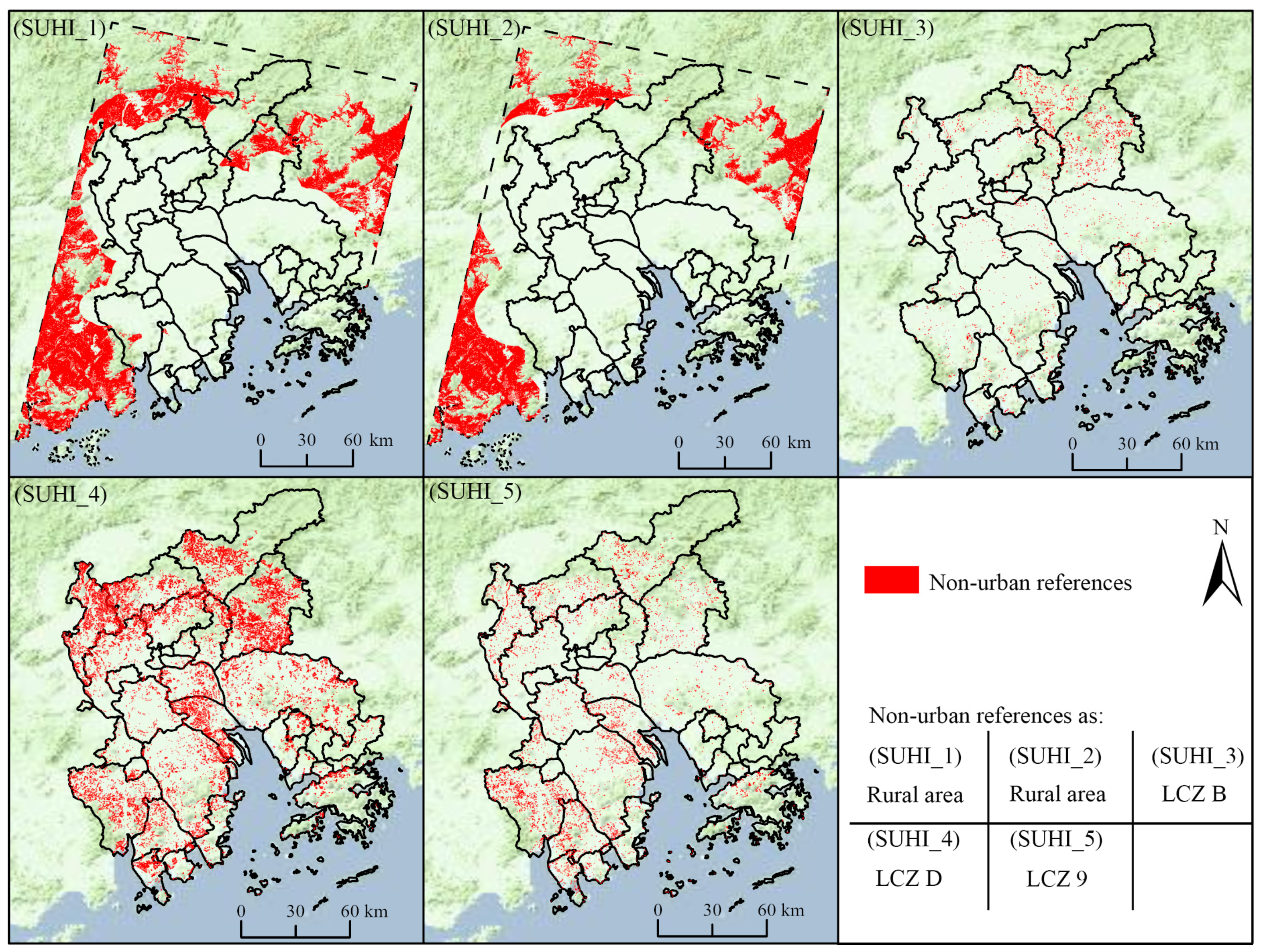
| SUHI Method | General Definition and Location | Excluded Factors | NSW LST | RTE LST |
|---|---|---|---|---|
| SUHI_1 | 10 km outside administrative non-urban areas | Water bodies and elevations exceeding ± 50 m of urban areas median elevation | 26.579 (SUHI_1N) | 29.009 (SUHI_1R) |
| SUHI_2 | 20 km outside administrative non-urban areas | Water bodies and elevations exceeding ± 50 m of urban areas median elevation | 26.593 (SUHI_2N) | 29.040 (SUHI_2R) |
| SUHI_3 | LCZ B | Elevations exceeding ± 50 m of urban areas median elevation | 26.263 (SUHI_3N) | 28.580 (SUHI_3R) |
| SUHI_4 | LCZ D | Elevations exceeding ± 50 m of urban areas median elevation | 27.078 (SUHI_4N) | 29.263 (SUHI_4R) |
| SUHI_5 | LCZ 9 | Elevations exceeding ± 50 m of urban areas median elevation | 27.488 (SUHI_5N) | 29.552 (SUHI_5R) |
| SUHI_6 | - | - | 26.800 (SUHI_6N) | 29.089 (SUHI_6R) |
| Type | SHUII | TRank | Grade | Type | SHUII | TRank | Grade |
|---|---|---|---|---|---|---|---|
| LCZ E | 4.219 | 1 | H | LCZ 5 | 1.950 | 16 | W |
| LCZ 10 | 3.872 | 2 | H | LCZ 1 | 1.859 | 17 | W |
| Commercial service | 3.282 | 3 | M | Educational | 1.777 | 18 | W |
| Industrial | 3.275 | 4 | M | Airport facilities | 1.621 | 19 | W |
| Transportation stations | 3.243 | 5 | M | Park and greenspace | 1.440 | 20 | I |
| LCZ 8 | 2.899 | 6 | M | LCZ 4 | 1.106 | 21 | I |
| Business | 2.678 | 7 | M | LCZ 6 | 0.725 | 22 | I |
| LCZ 3 | 2.606 | 8 | M | LCZ 9 | 0.203 | 23 | I |
| LCZ 2 | 2.540 | 9 | M | LCZ D | 0.103 | 24 | I |
| Medical | 2.509 | 10 | M | LCZ G | −0.076 | 25 | I |
| Sport and cultural | 2.401 | 11 | W | LCZ 7 | −0.224 | 26 | I |
| Mixed-use | 2.314 | 12 | W | LCZ A | −0.617 | 27 | I |
| Administrative | 2.287 | 13 | W | LCZ B | −1.147 | 28 | I |
| LCZ F | 2.237 | 14 | W | LCZ C | −1.947 | 29 | I |
| Residential | 2.151 | 15 | W |
| SUHI Scenarios | NUR_Standard | NUR_Water | NUR_DEM | |||
|---|---|---|---|---|---|---|
| NUR Scenarios | ALST | NUR Scenarios | ALST | NUR Scenarios | ALST | |
| SUHI_1N | NUR_1N_S | 26.579 | NUR_1N_W | 26.536 | NUR_1N_D | 26.349 |
| SUHI_2N | NUR_2N_S | 26.593 | NUR_2N_W | 26.546 | NUR_2N_D | 26.023 |
| SUHI_3N | NUR_3N_S | 26.263 | NUR_3N_W | 26.277 | NUR_3N_D | 25.253 |
| SUHI_4N | NUR_4N_S | 27.078 | NUR_4N_W | 27.061 | NUR_4N_D | 26.892 |
| SUHI_5N | NUR_5N_S | 27.488 | NUR_5N_W | 27.393 | NUR_5N_D | 27.185 |
| SUHI_6N | NUR_6N_S | 26.800 | NUR_6N_W | 26.763 | NUR_6N_D | 26.341 |
| SUHI_1R | NUR_1R_S | 29.009 | NUR_1R_W | 28.876 | NUR_1R_D | 28.578 |
| SUHI_2R | NUR_2R_S | 29.040 | NUR_2R_W | 28.903 | NUR_2R_D | 28.296 |
| SUHI_3R | NUR_3R_S | 28.580 | NUR_3R_W | 28.578 | NUR_3R_D | 27.684 |
| SUHI_4R | NUR_4R_S | 29.263 | NUR_4R_W | 29.195 | NUR_4R_D | 29.111 |
| SUHI_5R | NUR_5R_S | 29.552 | NUR_5R_W | 29.358 | NUR_5R_D | 29.299 |
| SUHI_6R | NUR_6R_S | 29.089 | NUR_6R_W | 28.982 | NUR_6R_D | 28.594 |
| SUHI Scenarios | SUHII | SUHI Scenarios | SUHII | ||
|---|---|---|---|---|---|
| LCZ | UFZ | LCZ | UFZ | ||
| SUHI_1N | 0.581 | 2.818 | SUHI_1R | 0.224 | 2.440 |
| SUHI_2N | 0.567 | 2.804 | SUHI_2R | 0.193 | 2.409 |
| SUHI_3N | 0.897 | 3.134 | SUHI_3R | 0.653 | 2.869 |
| SUHI_4N | 0.082 | 2.319 | SUHI_4R | −0.030 | 2.186 |
| SUHI_5N | −0.328 | 1.909 | SUHI_5R | −0.319 | 1.897 |
| SUHI_6N | 0.360 | 2.597 | SUHI_6R | 0.144 | 2.360 |
Disclaimer/Publisher’s Note: The statements, opinions and data contained in all publications are solely those of the individual author(s) and contributor(s) and not of MDPI and/or the editor(s). MDPI and/or the editor(s) disclaim responsibility for any injury to people or property resulting from any ideas, methods, instructions or products referred to in the content. |
© 2024 by the authors. Licensee MDPI, Basel, Switzerland. This article is an open access article distributed under the terms and conditions of the Creative Commons Attribution (CC BY) license (https://creativecommons.org/licenses/by/4.0/).
Share and Cite
Deng, H.; Zhang, S.; Chen, M.; Feng, J.; Liu, K. Sensitivity of Local Climate Zones and Urban Functional Zones to Multi-Scenario Surface Urban Heat Islands. Remote Sens. 2024, 16, 3048. https://doi.org/10.3390/rs16163048
Deng H, Zhang S, Chen M, Feng J, Liu K. Sensitivity of Local Climate Zones and Urban Functional Zones to Multi-Scenario Surface Urban Heat Islands. Remote Sensing. 2024; 16(16):3048. https://doi.org/10.3390/rs16163048
Chicago/Turabian StyleDeng, Haojian, Shiran Zhang, Minghui Chen, Jiali Feng, and Kai Liu. 2024. "Sensitivity of Local Climate Zones and Urban Functional Zones to Multi-Scenario Surface Urban Heat Islands" Remote Sensing 16, no. 16: 3048. https://doi.org/10.3390/rs16163048
APA StyleDeng, H., Zhang, S., Chen, M., Feng, J., & Liu, K. (2024). Sensitivity of Local Climate Zones and Urban Functional Zones to Multi-Scenario Surface Urban Heat Islands. Remote Sensing, 16(16), 3048. https://doi.org/10.3390/rs16163048