Joint Luminance-Saliency Prior and Attention for Underwater Image Quality Assessment

Abstract

Underwater images, as a crucial medium for storing ocean information in underwater sensors, play a vital role in various underwater tasks. However, they are prone to distortion due to the imaging environment, which leads to a decline in visual quality, which is an urgent issue for various marine vision systems to address. Therefore, it is necessary to develop underwater image enhancement (UIE) and corresponding quality assessment methods. At present, most underwater image quality assessment (UIQA) methods primarily rely on extracting handcrafted features that characterize degradation attributes, which struggle to measure complex mixed distortions and often exhibit discrepancies with human visual perception in practical applications. Furthermore, current UIQA methods lack the consideration of the perception perspective of enhanced effects. To this end, this paper employs luminance and saliency priors as critical visual information for the first time to measure the enhancement effect of global and local quality achieved by the UIE algorithms, named JLSAU. The proposed JLSAU is built upon an overall pyramid-structured backbone, supplemented by the Luminance Feature Extraction Module (LFEM) and Saliency Weight Learning Module (SWLM), which aim at obtaining perception features with luminance and saliency priors at multiple scales. The supplement of luminance priors aims to perceive visually sensitive global distortion of luminance, including histogram statistical features and grayscale features with positional information. The supplement of saliency priors aims to perceive visual information that reflects local quality variation both in spatial and channel domains. Finally, to effectively model the relationship among different levels of visual information contained in the multi-scale features, the Attention Feature Fusion Module (AFFM) is proposed. Experimental results on the public UIQE and UWIQA datasets demonstrate that the proposed JLSAU outperforms existing state-of-the-art UIQA methods.

1. Introduction

Underwater images serve as an important medium for transmitting ocean information, supporting autonomous underwater vehicles, remotely operated vehicles, and other marine instruments to help them efficiently complete tasks such as ocean resource exploration and deep-sea facility monitoring [1]. However, due to the unique properties of the underwater environment, the imaging process often suffers from light absorption and scattering, resulting in low contrast, color casts, haze effects, and other visual impediments that affect subsequent image processing systems in underwater instruments [2]. Consequently, extensive research on Underwater Image Enhancement (UIE) algorithms [3] has received significant attention, aiming to improve the visual quality of underwater images and aiding downstream tasks (i.e., saliency detection, object detection, image segmentation, etc.). However, due to the lack of high-quality underwater reference images, most existing UIE algorithms rely on synthetic datasets, and none are universally effective, limiting their applicability in real-world scenarios. Enhanced underwater images may still retain unresolved issues or introduce additional distortions, such as artifacts related to over-enhancement or detail loss related to under-enhancement. Therefore, Image Quality Assessment (IQA) [4,5,6,7] methods are often necessary for objective assessment, promoting the development of image systems for various optical sensors.

Thus far, many traditional in-air IQA methods have been proposed [8,9,10,11]. Among them, Mean Squared Error (MSE) and Peak Signal-to-Noise Ratio (PSNR) are classic Full Reference (FR) methods that often serve as benchmarks for optimizing UIE algorithms. However, MSE and PSNR, defined based on pixel-wise differences, fail to adequately capture features affecting human perception, such as texture details [12]. Given the unavailability of reference images in many cases, the application value of No-Reference (NR) IQA methods becomes more prominent. Existing NR-IQA methods primarily gauge image distortion by extracting Natural Scene Statistics (NSS) features in spatial or transform domains. These encompass classic NSS features, like Mean Subtracted Contrast Normalized (MSCN) coefficients [8], wavelet transformation coefficients [9], and discrete cosine transformation coefficients [10], among others, which have shown success in in-air images. However, due to the unique imaging environment, statistical NSS features change in underwater images, making it difficult to capture the increased noise and non-Gaussian distribution variations present in these images. Additionally, some progress has been made in deep learning (DL)-based IQA methods for in-air images [13,14,15,16,17,18,19,20]. For example, some methods utilize transfer learning [13] and meta-learning [16] to learn distortion features of in-air images, thereby achieving distortion classification and discrimination. However, the imaging characteristics and primary degradations of underwater images differ from those of in-air images. More importantly, the UIE algorithms may lead to more complex and variable artificial distortions of underwater images. Therefore, directly applying IQA methods designed for air images to evaluate underwater image quality may yield suboptimal results.

To this end, many traditional underwater IQA (UIQA) methods [21,22,23,24,25,26,27,28,29,30] have been proposed. Most of the existing traditional UIQA methods rely on extracting handcrafted features to reflect the distortion situations. For instance, methods like underwater color image quality evaluation (UCIQE) [21] gauge underwater image quality by extracting statistical features like chroma, saturation, and contrast from the CIELab color space, but do not consider any human perception factors. The underwater image quality measure (UIQM) [22], inspired by characteristics of the Human Vision System (HVS), incorporates measurements of colorfulness, sharpness, and contrast to evaluate underwater image degradation. However, the method of assigning manual weights to the extracted features to represent image quality has poor generalization and fails to adequately represent diverse degradation scenarios. Although these methods have a certain ability to assess common distortions such as low contrast and blurriness, they struggle to precisely quantify compound distortions caused by complex and dynamic underwater environments. Particularly, they inadequately perceive the intricate variations in color and structure introduced by UIE algorithms, like redshifts and artifacts. Due to the excellent feature learning capabilities of DL, some deep models for UIQA have been proposed [31,32,33]. Most of the DL-based UIQA methods use additional priors or conditions beyond the input to better learn the quality features. For example, some methods integrate color histogram priors as quality tokens to supplement global degradation information [31], but they fail to reflect the impact of local spatial structure on human perception. Others utilize depth maps as the weight to differentiate between foreground and background [32], but lack consideration of phenomena such as low contrast caused by luminance distortions. Previous works [34,35] used saliency maps as weights to measure perceptual quality. Typically, they directly apply or resize the saliency map to fit the required input size without delving into their inherent perceptual information. Although these embedded conditions or priors help the methods to understand the image quality to some extent, there is still a lack of sufficient consideration for the visual information introduced by UIE algorithms. Therefore, it is necessary to improve the UIQA methods to evaluate the quality of the enhanced underwater images more accurately.

In this paper, we propose a novel joint saliency–luminance prior UIQA model called JLSAU. Specifically, considering distortions at different scales, such as texture details and haze effects, a pyramid-structured backbone network is constructed to capture multi-scale distortion features. Additionally, to measure the impact of the UIE algorithms on visual information, luminance and saliency priors are incorporated into multi-scale features, where luminance prior and saliency prior reflect the enhancement effect of global and local quality information, respectively. To this end, the Luminance Feature Extraction Module (LFEM) is proposed to comprehensively measure the global distortion of luminance, which is highly sensitive to the HVS. It supplements multi-scale features to enhance the perception of global distortions, such as low contrast. Furthermore, the Saliency Weight Learning Module (SWLM) is designed to learn saliency features that reflect variations in local quality, serving as supplementary priors to enhance the perception of textures and details within multi-scale features. Finally, multi-scale features containing rich perceptual quality information are obtained and the AFFM based on attention mechanism is proposed to model the visual information at different levels. The experimental results show that, compared to existing UIQA methods, the proposed JLSAU has better performances for two different underwater image datasets. The main contributions of our work are summarized as follows:

• To enhance the global quality perception of multi-scale features, the LFEM is proposed to learn quality-aware representations of luminance distribution as prior knowledge. This includes learning quantitative statistical features through histogram statistics and designing a convolutional network to encode and supplement the positional information missing from the statistical features.
• To improve the local quality perception of multi-scale features, the SWLM is designed to extract saliency features in the channel and spatial domains as prior knowledge. These features reflect the enhancement effect of UIE algorithms on local quality, thereby enhancing the perception of structure and texture.
• To model the relationship of perceptual information among multi-scale features augmented by luminance and saliency prior, AFFM is introduced. It effectively integrates perception quality information from different levels of features using attention mechanisms, aiming to comprehensively perceive distortions in enhanced images.

2. Related Work

2.1. Underwater Image Enhancement Algorithms

Jaffe McGlamery [36] defines the underwater Image Forming Model (IFM) as a linear combination of direct reflection, background scattering, and forward scattering of light. The forward scattering is almost negligible. When only the direct scattering and the backscattering are considered, the underwater image ${\mathit{I}}_{\alpha }$ can be defined as follows:

$${\mathit{I}}_{\alpha }={\mathit{S}}_{\alpha }·{\mathit{\tau }}_{\alpha }+{\mathit{B}}_{\alpha }\left(1-{\mathit{\tau }}_{\alpha }\right)$$

(1)

where $\alpha \in \{R,G,B\}$ represents the color channel, ${\mathit{S}}_{\alpha }$ represents the original scene, ${\mathit{\tau }}_{\alpha }$ represents the transmission map, and ${\mathit{B}}_{\alpha }$ represents the background light.

Based on the involvement of IFM, Underwater Image Enhancement (UIE) algorithms can be categorized as model-based or model-free. Model-based algorithms typically rely on estimating parameters to reverse IFM. For instance, Peng et al. [37] estimated the background light, scene depth, and transmission map through blurriness and light absorption of underwater images. Zhao et al. [38] derived the relevant attenuation and scattering coefficients of RGB channels from the background color of underwater images for dehazing and color correction. However, parameter estimation often lacks sufficient constraints, requiring appropriate prior information for optimization. To address this issue, Drew et al. [39] introduced the underwater dark channel prior based on the characteristic that red light is more easily absorbed in water, which provides a good constraint for estimating the transmission map. The utilization of reasonable prior information and constraints has indeed improved the accuracy of parameter estimation to some extent. However, due to the complexity and variability of the underwater environment, significant estimation deviations still persist. For example, inaccurate depth estimation may result in structure distortion. In addition, to mitigate the impact of environmental factors on image degradation, some studies begun to explore extended IFM. For example, Li et al. [40] proposed an effective variational framework based on an extended IFM.

Model-free algorithms adopt direct pixel value adjustments to improve image quality. For example, Fu et al. [41] proposed a two-step UIE algorithm, incorporating color correction and contrast enhancement. Li et al. [42] decomposed underwater images into high- and low-frequency components, suppressing noise in the high-frequency component and adaptively enhancing color and contrast in the low-frequency component. Lu et al. [43] utilized a diffusion model for UIE, developing a new accelerated sampling method to optimize the probability distribution in the diffusion stage. Additionally, reinforcement learning-based UIE algorithms have made significant progress. For instance, Wang et al. [44] first introduced reinforcement learning into UIE algorithms by using UIQM as a feedback function and a positive learning direction. Sun et al. [45] modeled UIE as a Markov decision process, optimizing it based on reinforcement learning strategies. Wang et al. [46] proposed a reinforcement learning paradigm that controls actions to enhance visual effects and improve object detection performance, but it did not consider human perception factors. To address this, they later introduced a human visual perception-driven paradigm [47] and a method [48] that incorporates color priors into the scoring process. Moreover, some reinforcement learning methods are optimized based on visual preferences, such as the Meta underwater camera [49], which uses reinforcement learning strategies to globally optimize the configuration of parameter values in a comprehensive cascade of UIE methods. There is also a framework [50] that fine-tunes and improves hierarchical probability networks using reinforcement learning. Additionally, the Metalantis framework [51] supports IFM through reinforcement learning with virtually generated data. However, these reinforcement learning-based UIE algorithms, which use image quality as a reward, are limited by the performance of UIQA. Although these algorithms have improved underwater image quality to some extent, the complexity of the underwater imaging environment makes it challenging to completely restore image details. Additionally, these algorithms may introduce additional distortions, such as red offsets, artifacts, and structure loss, resulting in no substantial improvement in visual quality. Therefore, appropriate visual quality assessment methods are necessary to evaluate and enhance the performance of UIE algorithms.

2.2. Underwater Image Quality Assessment

In recent years, Image Quality Assessment (IQA) has made significant strides in in-air images [9,10,11,12,13,14,15,16,17,18,19,20]. Among them, Peak Signal-to-Noise Ratio (PSNR), Mean Square Error (MSE), and Structural Similarity Index Measure (SSIM) [52] are commonly used as Full Reference (FR) metrics for optimizing and evaluating UIE algorithms. Since FR-IQA requires reference images that are often unavailable, studying No Reference (NR) IQA methods becomes more practically significant. For in-air images, numerous NR-IQA methods based on Natural Scene Statistics (NSS) have been developed. For example, Mittal et al. [8] proposed the use of Blind/Referenceless Image Spatial Quality Evaluator (BRISQUE), which quantifies naturalness using NSS features of local normalized brightness coefficients without frequency domain decomposition. Moorthy et al. [9] proposed an NR-IQA method called Distortion Identification-based Image INtegrity and Verity Evaluation (DIIVINE), which extracts NSS features in the wavelet domain to identify image distortion types. Since deep learning (DL) can automatically learn image distortion features, attention has shifted to DL-based NR-IQA methods [13,14,15,16,17,18,19,20]. For example, Kang et al. [14] designed a Convolutional Neural Network (CNN)-based method that represents overall quality by predicting the quality of image patches. Su et al. [16] introduced a meta-learning based method, called Meta-IQA, which adapts to real unknown distortions by learning shared meta-knowledge. Meanwhile, Golestaneh et al. [17] developed an evaluation model using a hybrid structure of CNN and Transformer, incorporating relative ranking loss and self-consistency loss as constraints. However, due to the distinct imaging environments and principles of underwater versus in-air images, there are significant differences in the types and levels of distortion. Therefore, IQA methods designed for in-air images may not perform optimally for evaluating underwater images.

To address the unique distortions in underwater images and gain insights into UIE algorithm development, Yang et al. [21] proposed an NR method, called Underwater Color Image Quality Evaluation Metric (UCIQE), which is a linear combination of chrominance, saturation, and contrast. It quantitatively measures distortions such as color shift, blur, and low contrast, but lacks sufficient consideration of human visual perception-related factors. Inspired by the properties of HVS, Panetta et al. [22] introduced the underwater image quality measure (UIQM), which includes three components, i.e., color measurement, sharpness measurement, and contrast measurement. However, linear weighting of handcrafted features still struggles to accurately capture the diversity of degradation types and degrees in underwater images. Then, Wang et al. [23] quantified color loss, blur, and haze effects by analyzing the influence of light absorption and scattering. Jiang et al. [24] derived quality-aware features from chrominance and luminance components for assessing color shift, inadequate luminosity, and degradation of sharpness or detail. Yang et al. [25] combined with human visual perception properties, proposed a method that considers the degradation effects in underwater images, albeit overlooking naturalness and structural information. Zheng et al. [26] introduced the Underwater Image Fidelity (UIF) method, which extracts the statistical features from the CIElab space to construct naturalness, sharpness, and structure indicators, yet disregards color information. Li et al. [27] extracted statistical features based on underwater dark channel and underwater bright channel priors in their proposed method. In contrast to prior approaches focusing on a limited set of image attributes, Liu et al. [28] developed six quality perception features aimed at providing a more comprehensive evaluation of luminance, sharpness, color balance, contrast, haze density, and noise. Zhang et al. [29] introduced a series of quality awareness features, including naturalness, color, contrast, clarity, and structure. Hou et al. [30] introduced new measures of contrast, clarity, and naturalness for underwater images. Although traditional UIQA methods based on handcrafted features have achieved some success, DL-based methods have gradually gained public attention due to their performance advantages.

In recent years, some DL-based methods have been proposed, using additional priors or conditions. For example, Guo et al. [31] utilized the RGB color histogram prior as an embedding feature to supplement global degradation information, combined with a dynamic cross-scale correspondence module for multi-scale feature fusion. Nevertheless, the histogram prior derived solely from pixel statistics fails to reflect the impact of different color information within specific spaces and structures on human perception. Li et al. [32] considered the impact of spatial information on local quality by using the depth map prior as a weight to guide the model in distinguishing foreground–background differences. Fu et al. [33] generated samples of varying qualities by linear mixing and trained a Siamese network using a self-supervised mechanism to learn quality ranking. However, they did not consider cases of over-enhancement introduced by UIE algorithms, leading to artifacts and other issues. Despite this, most UIQA methods are still primarily based on basic visual features, such as saturation and sharpness, lacking consideration for HVS characteristics and their relevance to downstream tasks. Therefore, this paper focuses on the changes in saliency detection tasks brought about by the enhancement effects of UIE and combines human visual characteristics to propose the JLSAU method.

3. The Proposed Method

To capture the distortion present in enhanced underwater images, we propose a novel multi-scale UIQA model named JLSAU, with a joint luminance–saliency prior. To focus on the variations in image saliency caused by local distortions, saliency features are extracted as visual weights to measure local perceptual quality. Additionally, the perceptual quality representation of luminance information is learned by extracting grayscale histogram statistical features, and positional information is supplemented. Finally, considering the multi-scale perceptual characteristics of HVS, a fusion module based on the attention mechanism is constructed to model the distortion information between different scale features. The overall framework of the proposed JLSAU is shown in Figure 1. In this section, the key parts of JLSAU will be explained in detail, including its pyramid-structured backbone (hereinafter referred to as backbone), Luminance Feature Extraction Module (LFEM), Saliency Weight Learning Module (SWLM), Attention Feature Fusion Module (AFFM), and loss function setting.

3.1. Backbone

Enhanced underwater images not only include distortions caused by the inherent properties of the water medium, but also artificial distortions introduced by UIE algorithms. The distortions can be categorized at different scales into local distortions, such as structure loss, artifacts, and false edges, as well as global distortions, such as low contrast and color deviations. To capture the different scales of distortion information, we design a pyramid structure module as the backbone for JLSAU. The backbone extracts multi-scale features from the RGB space containing abundant raw color information. The extracted multi-scale features contain rich perceptual quality information such as color, texture, etc. The backbone consists of four stages. Each stage is composed of a downsampling layer, a Multi-Scale Conv Attention (MSCA), and a Feed-Forward Network (FFN). To reduce information loss, overlapping convolution is used instead of pooling for downsampling, which also facilitates modeling the local continuity of structural information. The MSCA consists of a batch normalization layer, a depth-wise convolution, multi-branch strip convolutions, and a 1 × 1 convolution. As shown in Figure 1, MSCA can be represented as follows:

$$MSCA\left(x\right)=Con{v}_{1\times 1}\left(\sum _{n=1}^{4}Scal{e}_n\left(Con{v}_{\mathrm{dw}}\left(BN\left(x\right)\right)\right)\right)\odot BN\left(x\right)$$

(2)

where $\mathit{x}$ represents the input feature, ⊙ represents the element-wise matrix multiplication, $\mathit{BN}(·)$ represents batch normalization, ${\mathit{Conv}}_{1\times 1}(·)$, and ${\mathit{Conv}}_{\mathrm{dw}}(·)$ represent $1\times 1$ convolution and depth-wise convolution, respectively, and ${\mathit{Scale}}_n(·)$ represents the n-th branch of multi-branch strip convolutions, where $n\in \{1,2,3,4\}$.

Specifically, depth-wise convolution aggregates local information, multi-branch strip convolutions capture multi-scale features, and 1 × 1 convolution aggregates the information between channels. FFN is composed of BN-Conv-Gelu-Conv, serving to efficiently integrate and transform channel-wise features, enhancing the representational power of the network for each stage. Finally, the output features are obtained during every stage, denoted as ${\mathit{f}}_i\in {\mathbb{R}}^{C_i\times H_i\times W_i}$, where $i\in \{1,2,3,4\}$ represents stages $C_i$ and $H_i$ and $W_i$ represent the number of channels, height, and width of the feature maps at the i-th stage, respectively.

3.2. Luminance Feature Extraction Module

Underwater images typically exhibit global distortions such as low contrast and low visibility in terms of luminance, which significantly affects their quality. To analyze the performance of enhanced underwater images of varying quality in terms of luminance attributes, adaptive histogram equalization is applied. Histogram equalization can distribute pixel values uniformly across the entire luminance range, enhance image contrast, and improve detail. As shown in Figure 2, four groups of enhanced underwater images and their corresponding histogram equalization results are selected from the UIQE dataset. Each group includes enhanced images obtained by different UIE algorithms that vary from low quality to high quality. Obviously, compared to low-quality images, high-quality images exhibit smaller differences before and after processing, resulting in higher visual similarity. Conversely, the global distortions such as low contrast in low-quality images have been significantly improved. Viewing histogram equalization as a mapping process, the mapping distance between the before and after results can reflect image similarity and thereby indicate image quality. Thus, given an enhanced underwater image $\mathit{I}$ and its histogram equalization result $\overline{\mathit{I}}$, the difference between them can reflect the quality of $\mathit{I}$. To quantify the difference, LFEM is designed to extract high-dimensional luminance features containing differential information.

Specifically, $\mathit{I}$ and $\overline{\mathit{I}}$ are transferred to grayscale and the results are denoted as ${\mathit{I}}_{\mathrm{g}}$ and ${\overline{\mathit{I}}}_{\mathrm{g}}$. Let ${\overline{\mathit{I}}}_{\mathrm{diff}}$ be the difference map obtained by subtracting ${\mathit{I}}_{\mathrm{g}}$ from ${\overline{\mathit{I}}}_{\mathrm{g}}$, which serves as the input of the LFEM. Then, the statistical features of ${\overline{\mathit{I}}}_{\mathrm{diff}}$ are obtained through histogram statistics, which are sent into a fully connected layer to obtain the final luminance statistical vector, denoted as ${\mathit{V}}_{\mathrm{L}}$. It can be expressed as follows:

$${\mathit{V}}_{\mathrm{L}}=FC\left(histogram\left({\overline{\mathit{I}}}_{\mathrm{diff}}\right)\right)$$

(3)

where $histogram(·)$ represents the histogram statistical operation in the grayscale space, and $FC(·)$ represents the fully connection.

Histogram statistics only capture the quantitative statistical relationship of grayscale levels without providing the specific spatial information of pixels. Inspired by the encoding ability of the convolution layer with the relative position [53], a convolutional branch is designed for implicit position encoding. Specifically, it comprises three stages, each comprising an LFE block (i.e., Conv-ReLU-Conv layer), a skip connection, and a downsampling layer. The LFE block not only captures local features but also preserves the spatial context, allowing the network to infer relative positions implicitly, which can be expressed as follows:

$${\mathit{u}}_{i+1}=down\left(Conv\left(ReLU\left(Conv\left({\mathit{u}}_i\right)\right)\right)+{\mathit{u}}_i\right)$$

(4)

where $i\in \{1,2,3\}$ represents the number of stages, ${\mathit{u}}_i$ represents the output of the convolutional branch at stage i, ${\mathit{u}}_1$ is equivalent to ${\overline{\mathit{I}}}_{\mathrm{diff}}$, $\mathit{down}(·)$ represents downsampling, and $\mathit{Relu}(·)$ represents the ReLU activation function.

Subsequently, due to the subsequent processes not involving the handling of the variable whose subscript i is 1, to avoid ambiguity and describe concisely, the subscript i will be replaced with $\lambda$ below, where $\lambda \in \{2,3,4\}$. The obtained features ${\mathit{u}}_{\lambda }$ are subjected to a mapping operation that includes global max pooling and convolutional layers to obtain multi-scale luminance features ${\mathit{L}}_{\lambda }$, which can be expressed as follows:

$${\mathit{L}}_{\lambda }=Conv\left(GMP\left({\mathit{u}}_{\lambda }\right)\right)$$

(5)

where $\mathit{GMP}(·)$ represents global max pooling.

Finally, by pixel-wise multiplication with ${\mathit{L}}_{\lambda }$ containing relative position information, multi-scale features ${\mathit{f}}_{\lambda }$ are supplemented with luminance information, which can be expressed as follows:

$${\widehat{\mathit{f}}}_{\lambda }={\mathit{f}}_{\lambda }\odot {\mathit{L}}_{\lambda }$$

(6)

3.3. Saliency Weight Learning Module

Influenced by attributes such as color, contrast, and texture, human perception tends to focus on certain parts of a scene, namely regions of saliency. Saliency detection and UIQA are essentially related, as they both depend on how HVS perceives images. If visual saliency is affected, it implies a change in visual quality. Moreover, visual salient regions are also crucial aspects that UIQA needs to consider. 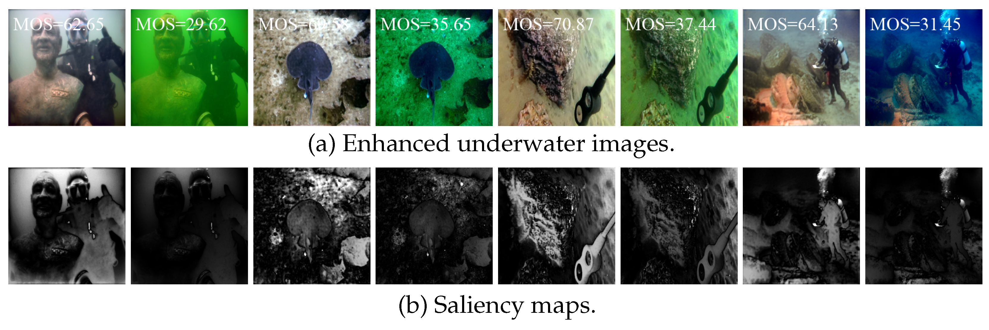Figure 3 shows different enhanced underwater images and their corresponding saliency maps, including two control groups of high and low quality. It can be observed that different enhancement effects lead to varying degrees of improvement in the results of saliency detection, which can reflect the quality of the input enhanced images. Therefore, to better perceive local quality, SWLM is designed to extract saliency features. This module indirectly reflects image-quality changes introduced by UIE algorithms and assigns visual weights to different regions. The specific framework is shown in Figure 4.

Firstly, the method proposed by Montalone [54] is utilized to calculate the saliency map. For an enhanced underwater image $\mathit{I}$, its saliency map is denoted as ${\mathit{I}}_s$, which is input into two convolutional-activation layers to expand channel dimensions and obtain low-level saliency features ${\overline{\mathit{I}}}_s$, which can be represented as follows:

$${\overline{\mathit{I}}}_s=Relu\left(Conv\left(Relu\left(Conv\left({\mathit{I}}_s\right)\right)\right)\right)$$

(7)

Then, a dual-branch network is designed to obtain the perceptual features of ${\overline{\mathit{I}}}_s$ in both spatial and channel. The spatial branch aims to capture complex spatial relationships, while the channel branch aims to capture uneven channel degeneration. For the channel branch, it includes a global average pooling layer and a global max pooling layer to refine the feature, followed by a fully connected layer and sigmoid activation function to generate channel weights $\mathit{V}$, which can be expressed as follows:

$$\mathit{V}=Sig\left(FC\left(GAP\left({\overline{\mathit{I}}}_s\right)\copyright GMP\left({\overline{\mathit{I}}}_s\right)\right)\right)$$

(8)

where $\mathit{Sig}(·)$ represents the sigmoid activation function, $\mathit{GAP}(·)$ represents global average pooling, and © represents splicing on a specific dimension.

For the spatial branch, it contains an average pooling layer and a max pooling layer, followed by a convolution layer and sigmoid activation function to obtain the spatial weight $\mathit{M}$, which can be expressed as follows:

$$\mathit{M}=Sig\left(Conv\left(AP\left({\overline{\mathit{I}}}_s\right)\copyright MP\left({\overline{\mathit{I}}}_s\right)\right)\right)$$

(9)

where $\mathit{AP}(·)$ and $\mathit{MP}(·)$ represent average pooling and max pooling, respectively.

To maintain correspondence with the size of the multi-scale feature ${\widehat{\mathit{f}}}_{\lambda }$, ${\mathit{M}}_{\lambda }$ and ${\mathit{V}}_{\lambda }$ are obtained by adjusting the output dimension of $\mathit{FC}(·)$ and the convolution kernel size of $\mathit{Conv}(·)$. Finally, the feature ${\widehat{\mathit{f}}}_{\lambda }$ is weighted with the corresponding ${\mathit{M}}_{\lambda }$ and ${\mathit{V}}_{\lambda }$ obtained from the saliency prior, and concatenated on the channel dimension to obtain weighted features ${\overline{\mathit{f}}}_{\lambda }$, which can be expressed as follows:

$${\overline{\mathit{f}}}_{\lambda }=\left({\widehat{\mathit{f}}}_{\lambda }\odot {\mathit{V}}_{\lambda }+{\widehat{\mathit{f}}}_{\lambda }\right)\copyright \left({\widehat{\mathit{f}}}_{\lambda }\odot {\mathit{M}}_{\lambda }+{\widehat{\mathit{f}}}_{\lambda }\right)$$

(10)

3.4. Attention Feature Fusion Module

Feature fusion, as a common component of DL models, typically integrates low-level and high-level features through long skip connections or summation to obtain features with high resolution and strong semantic information [55]. Finding the appropriate fusion method is crucial for achieving the desired goals for different tasks. For UIQA, the HVS exhibits multi-scale perception characteristics, where features at different scales have complementary advantages. Low-level features possess a small receptive field, demonstrating strong representations of geometric details that can reveal texture structure distortion. Conversely, high-level features have large receptive fields and a robust ability to represent semantic information, capturing global distortions such as the haze effect. To this end, considering that employing an attention module can enhance the understanding of contextual information within complex features and emphasize more important parts [56,57,58], we propose an attention-based fusion module that is used to model the distortion information contained between multi-scale features. The main framework is illustrated in Figure 5.

Firstly, to achieve dimensional transformation and feature extraction, the input feature is divided into fixed-size patches and linearly mapped, thus enabling the capture of essential representations for subsequent relationship modeling. Multi-scale feature ${\overline{\mathit{f}}}_{\lambda }$ has different receptive fields and resolutions. To ensure the mapped patches maintain consistency in image content, different convolutions are used for patch embedding, followed by a flattened layer to reduce the dimension. The size of the convolution kernel is consistent with the patch size, and the number of output channels is consistent with the embedding size. After feature mapping, the spatial and channel attention are calculated independently. Spatial attention is used to model multi-scale contextual information as local features, enhancing expressive ability. Different scales of contextual information help capture the relationship between structure and texture in enhanced images. Then, the spatial attention feature ${\mathit{F}}_s$ is obtained as follows:

$${\mathit{F}}_s=\mathrm{Softmax}\left({\displaystyle \frac{l\left({\overline{\mathit{f}}}_2\right)l{\left({\overline{\mathit{f}}}_3\right)}^T}{\sqrt{\mathit{d}}}}\right)l\left({\overline{\mathit{f}}}_4\right)$$

(11)

where $l(·)$ represents linear mapping, $\mathit{Softmax}(·)$ represents the softmax function, $\sqrt{\mathit{d}}$ represents the square root of the feature dimension, and T represents transpose.

In addition, to model the interdependence between different channels and improve the perception of key channel information, we utilize channel attention feature ${\mathit{F}}_c$, which is obtained as follows:

$${\mathit{F}}_c=\mathrm{Softmax}\left({\displaystyle \frac{\mathit{l}{\left({\overline{\mathit{f}}}_2\right)}^{T}l\left({\overline{\mathit{f}}}_3\right)}{\sqrt{\mathit{d}}}}\right)l\left({\overline{\mathit{f}}}_4\right)$$

(12)

Finally, the perceptual feature $\mathit{F}$ is obtained by element-wise addition ${\mathit{F}}_c$ and ${\mathit{F}}_s$, which can be expressed as follows:

$$\mathit{F}={\mathit{F}}_c+{\mathit{F}}_s$$

(13)

3.5. Regression

By combining the luminance statistical vector ${\mathit{V}}_{\mathrm{L}}$ and perceptual feature $\mathit{F}$, the final quality feature is obtained, which is then input into the fully connected layer to calculate the final quality score S, which can be expressed as follows:

$$S=FC\left(\mathit{F}\odot {\mathit{V}}_{\mathrm{L}}\right)$$

(14)

The optimization of perceived quality prediction results employs MSE as the loss function $L_{\mathrm{MSE}}$, which can be expressed as follows:

$$L_{\mathrm{MSE}}={\displaystyle \frac{1}{N}}\sum _{i=1}^N{\left(Q-S\right)}^2$$

(15)

where S represents the quality predicted by the proposed JLSAU, and Q represents the Mean Opinion Score (MOS).

4. Experimental Results and Analysis

In this section, we first introduce the experimental settings in detail, including datasets, specific implementation details, and criteria for performance evaluation. Through comparison with a series of state-of-the-art IQA methods, the superior performance of JLSAU has been demonstrated, and is accompanied by extensive ablation studies to validate the contributions of key modules within JLSAU.

4.1. Experimental Settings

4.1.1. Datasets

UIQE [27] dataset, UWIQA [25] and UID2021 [59] datasets are used to train and test the proposed JLSAU. These datasets are composed of real underwater images and enhancement results of various UIE algorithms, with each enhanced image having a Mean Opinion Score (MOS) serving as the ground truth. Specifically, the UIQE dataset contains 405 images derived from 45 real underwater images processed by nine representative UIE algorithms. Each real underwater image and its enhanced results are regarded as a scene, and their MOS values are obtained using a five-level classification scale in a laboratory environment, with the scale administered by 25 volunteers employing a dual stimulus strategy. The UWIQA dataset contains 890 real underwater images with varying degrees of distortion, covering a variety of underwater scenes and common distortion types of underwater images. The MOS value for each image is derived by averaging the ratings from three assessments conducted in a laboratory environment by 21 observers with relevant expertise, following outlier removal. The UID2021 dataset consists of 960 images, including 60 scenes and enhanced results from 15 UIE algorithms, covering six common underwater scenes. The annotations for the UID2021 dataset are obtained through pairwise comparison and sorting by 52 observers in a laboratory environment.

4.1.2. Implementation Details

The dataset is randomly split into a training set and a testing set in a ratio of 8:2 based on scenes. During the training phase, data augmentation techniques, such as random horizontal flipping and random rotation, are applied to enhance the dataset. The enhanced images are segmented by clipping strategy, resulting in image patches of size 3 × 192 × 192, which serve as the input. The proposed JLSAU is implemented based on the PyTorch and trained on an NVIDIA RTX 3080 GPU. The Adam optimizer is used for optimization. The initial learning rate is set to $8\times {10}^{-4}$ and is updated by the cosine annealing strategy. MSE is employed as the loss function, and the batch size is set to 16, with a total of 300 epochs during training.

4.1.3. Evaluation Criteria

The performance of the proposed JLSAU is evaluated using three widely recognized indicators, including Spearman Rank Order Correlation Coefficient (SROCC), Kendall Rank Order Correlation Coefficient (KROCC), and Pearson Linear Correlation Coefficient (PLCC). These indicators measure the consistency between the score predicted by the objective method and the subjective MOS. Specifically, SROCC and KROCC are utilized to evaluate the accuracy of image quality prediction ranking, while PLCC measures the precision of objective score prediction. When SROCC, PLCC, and KROCC values approach 1, it indicates a higher consistency between the predicted quality scores and human subjective perception of quality.

4.2. Performance Comparisons

To establish the superiority of the proposed JLSAU, a variety of mainstream NR-IQA methods are selected for comparison. These includes two categories of methods, i.e., in-air IQA and UIQA. The in-air methods include DIIVINE [9], BRISQUE [8], BMPRI [11], CNN-IQA [14], TReS [17], and HyperIQA [19]. UIQA methods consist of UIQM [22], UCIQE [21], CCF [23], FDUM [25], UIQEI [27], NUIQ [24], Twice-Mixing [33], Uranker [31], UIQI [28], and CSN [30]. Both categories include methods based on traditional regression and deep learning. To ensure a fair comparison, all experiments are conducted using the source code published by the respective authors. For traditional regression methods, their source code is used to extract handcrafted features and then retrain support vector machines (SVMs) under the same conditions. For DL-based methods, the testing principles align with those of the proposed JLSAU, and network parameters are optimized to achieve the best performance.

Table 1. Performance comparison of different IQA methods on the UIQE and UWIQA datasets.

		Method	UIQE			UWIQA
			SROCC ↑	KROCC ↑	PLCC ↑	SROCC ↑	KROCC ↑	PLCC ↑
In-air IQA	Traditional	DIIVINE [9]	0.1278	0.1084	0.0997	0.4399	0.2915	0.3724
		BRISQUE [8]	0.7278	0.5000	0.7507	0.3456	0.2562	0.3669
		BMPRI [11]	0.6152	0.4167	0.6020	0.6815	0.4964	0.6875
	DL-based	CNN-IQA [14]	0.7840	0.5849	0.7765	0.6158	0.4711	0.5327
		TReS [17]	0.8721	0.6924	0.8845	0.6720	0.5365	0.6817
		HyperIQA [19]	0.7114	0.5841	0.7288	0.6501	0.5040	0.6799
Underwater IQA	Traditional	UIQM [22]	0.1556	0.1984	0.3112	0.6180	0.4730	0.6080
		UCIQE [21]	0.3254	0.2248	0.4551	0.6220	0.4740	0.5950
		CCF [23]	0.2556	0.1517	0.3010	0.4790	0.3510	0.4090
		FDUM [25]	0.2343	0.1685	0.3030	0.6830	0.5300	0.6380
		UIQEI [27]	0.8568	0.6456	0.8705	N/A	N/A	N/A
		NUIQ [24]	0.4433	0.3067	0.4023	0.4651	0.3766	0.4702
		UIQI [28]	0.7131	0.5157	0.7270	0.7423	0.5912	0.7412
		CSN [30]	0.7265	0.5258	0.7422	0.7423	0.6014	0.7648
	DL-based	Twice-Mixing [33]	0.5690	0.4142	0.5506	0.4727	0.3501	0.4422
		Uranker [31]	0.8188	0.6504	0.8172	0.5289	0.3992	0.5135
		Proposed	0.9102	0.7433	0.9233	0.7669	0.6193	0.7836

shows the performance comparison results for the UIQE dataset and the UWIQA dataset. For each column of comparative indicators, the best results are highlighted in bold. For the UIQE dataset, the proposed JLSAU demonstrates the best performance, with SROCC, KROCC, and PLCC reaching 0.9102, 0.7433, and 0.9233, respectively. For traditional in-air IQA methods, most of them, like DIIVINE, have poor performance, showing weak correlations. Even the best-performing traditional method, BRISQUE, still has a large gap with the proposed JLSAU, with SROCC as 0.7278, KROCC as 0.5000, and PLCC as 0.7507. The reasons can be analyzed as follows: traditional in-air IQA methods are mostly based on the NSS features of in-air images, which have good applicability and reliability in the atmosphere environment. However, there are significant differences in the forms and degrees of degradation between underwater and in-air images. The differing distortion statistical distributions make traditional NSS features unable to accurately reflect the perceived quality of underwater images. In addition, the performance of the proposed JLSAU is better than all the comparing UIQA methods. Compared with the best-performing UIQEI method in UIQA with SROCC, KROCC, and PLCC are 0.8568, 0.6456, and 0.8705, respectively, JLSAU achieves gains of nearly 6.25%, 15.14%, and 6.06% in the former three indicators, respectively. Most of the UIQA methods have limited generalization on the UIQE dataset. In particular, although the traditional UIQA methods (i.e., UIQM, UCIQE, CCF) were proven to have good performance in most underwater scenes at that time, they had a poor correlation with human perception in predicting the quality of enhanced underwater images. Although FDUM designed for raw underwater images is a recently proposed method, it lacks generalization performance when applied to enhanced underwater images. This may be due to the rapid development of UIE algorithms in recent years, as they have introduced complex color and structural changes in the enhanced underwater images that traditional UIQA methods cannot perceive. Additionally, CSN and UIQI attain the fourth and fifth position in the UIQA methods, demonstrating a certain degree of predictive accuracy. This may be attributed to the introduction of visual saliency by CSN, which is more consistent with human perception, while UIQI is attributed to consideration of a broader spectrum of attributes in enhanced underwater images. Finally, apart from Twice-Mixing, most DL-based methods (i.e., CNN-IQA, TReS, HyperIQA, Uranker) can achieve better performance and generalization ability than traditional methods. This is because Twice-Mixing performs the mixing in a way that cannot fit the uniform of the HVS and cannot cover the over-enhanced cases, whereas DL-based methods automatically learn high-level features and representations from images, enabling them to better capture high-quality information. Despite potential challenges such as model complexity and hyperparameter settings, DL-based methods generally outperform traditional methods in UIQA tasks. Fortunately, the proposed JLSAU achieves the best performance by considering the distortion characteristics of enhanced underwater images and incorporating knowledge about the priors of HVS.

To further validate the superiority and generalization of the proposed JLSAU, a comparative test is carried out on the UWIQA dataset. Unlike the UIQE dataset, the UWIQA dataset is composed of various real underwater images that have not been enhanced, featuring a richer variety of underwater scenes and diverse image sizes. As shown in Table 1, currently, various IQA methods exhibit mediocre performance on the UWIQA dataset, indicating that UIQA remains a challenge in the evaluation of real underwater images. The proposed JLSAU achieves competitive prediction performance, with the SROCC and PLCC values reaching 0.7669 and 0.7836—about 3.31% and 2.46% higher than the second-best CSN method, with SROCC reaching 0.7423 and PLCC reaching 0.7648, respectively. The results of other comparison methods are basically consistent with those on the UIQE dataset. The traditional in-air IQA methods perform poorly when predicting underwater images, and most of the DL-based methods are better than those traditional methods, whether for underwater or in-air images. It is worth mentioning that compared with the UIQE dataset, the traditional UIQA methods (i.e., UIQM, UCIQE, CCF, FDUM) show better performance. This is because the UWIQA dataset is composed of original underwater images without the uncertainty introduced by the UIE algorithms. In a word, compared to existing comparative methods, the proposed JLSAU has advantages in evaluating the perceptual quality of underwater images. The good performance of these two datasets proves the superiority of the proposed JLSAU.

In addition, we also conduct comparison experiments on the large-scale underwater dataset UID2021. Note that UIQEI is not open source and cannot be compared; the remaining comparison methods are consistent with those included in Table 1. As shown in

Table 2. Performance comparison of different IQA methods on the UID2021 dataset.

		Method	UID2021
			SROCC ↑	KROCC ↑	PLCC ↑
In-air IQA	Traditional	DIIVINE [9]	0.6112	0.4363	0.6264
		BRISQUE [8]	0.4689	0.3192	0.4794
		BMPRI [11]	0.5455	0.3823	0.5524
	DL-based	CNN-IQA [14]	0.6257	0.4766	0.6039
		TReS [17]	0.8335	0.6491	0.8304
		HyperIQA [19]	0.8022	0.6073	0.7864
Underwater IQA	Traditional	UIQM [22]	0.5349	0.3785	0.5689
		UCIQE [21]	0.5892	0.4340	0.6335
		CCF [23]	0.4577	0.3314	0.5371
		FDUM [25]	0.6406	0.4589	0.6464
		NUIQ [24]	0.7168	0.5293	0.7266
		UIQI [28]	0.6921	0.5093	0.6794
		CSN [30]	0.7210	0.5157	0.7157
	DL-based	Twice-Mixing [33]	0.6952	0.5113	0.7060
		Uranker [31]	0.7279	0.5448	0.7261
		Proposed	0.7467	0.5509	0.7353

, the proposed JLSAU achieves the best performance among various UIQA methods. This indicates that even in datasets with richer scenes and more comprehensive distortion coverage, the proposed JLSAU still has certain advantages. However, among all the methods compared, TReS achieves the best results. This may be due to the fact that TReS pay more attention to the relative distance information between each batch of images during design and have a stronger ability to sort relative quality. This ability is amplified when the training data are expanded. This insight is valuable for future considerations in designing UIQA methods.

At the same time, to visually demonstrate the performance comparison results, Figure 6 shows the scatter plot of subjective MOS values versus the predicted results of the proposed JLSAU on the UIQE testing set, along with those of other comparison methods. To provide an intuitive comparison within a reasonable length, we chose the top two traditional in-air IQA methods (i.e., BRISQUE, BMPRI), the top two DL-based in-air IQA methods (i.e., CNN-IQA, TReS), and top two DL-based UIQA methods (i.e., UIQEI, JLSAU) to plot the scatter plot. In the scatter plot, the y-axis represents the predicted scores and the x-axis represents the subjective MOS values. Clearly, a scatter plot demonstrating better prediction results should have points that are closer to the fitting curve. It can be easily observed from Figure 6 that the proposed JLSAU produces the best-fitting results on the UIQE dataset, with predicted objective scores closer to the subjective MOS values.

To further demonstrate the ability of the proposed JLSAU to perceive distortion in the enhanced underwater images, a series of images are chosen from the UIQE testing set. The predicted scores from different methods along with the corresponding MOS values are provided, (i.e., from left to right: JLSAU, BRISQUE, BMPRI, CNN-IQA, TReS, and UIQEI). Note that the number in parentheses represents the predicted ranking of the corresponding method for this scene, and methods with correct rankings are highlighted in red. As shown in Figure 7, the images are arranged from left to right based on MOS values, with perceptual quality ranging from low to high. It is evident that the enhanced images closer to the left exhibit lower overall visual perceptual quality, with most of them showing inadequate enhancement and severe global distortions, such as color distortion and low contrast. As enhancement improves, the perceptual quality of the underwater images gradually increases, addressing issues like color shifts and low contrast, while local details and texture structures become clearer. In Figure 7, for the enhanced images of the same scene, the proposed JLSAU provides an accurate objective ranking. Although the TReS also provides the correct ranking, the scores obtained by JALSU are generally closer to the MOS values, which enables accurate differentiation of the enhancement quality from good to poor. However, most other methods exhibit a wide range of predicted quality for enhanced underwater images at different levels within the same scene, failing to perceive subtle changes and trends, particularly BMPRI and BRISQUE, while TReS and UIQEI perform relatively better in their predictions.

4.3. Ablation Experiment

The proposed JLSAU consists of several key components: SWLM, LFEM, and AFFM.

Table 3. Ablation experiments on the effects of different components.

Method	SWLM	LFEM	AFFM	UIQE			UWIQA
				SROCC	KROCC	PLCC	SROCC	KROCC	PLCC
(a)	✔	✔		0.9049	0.7412	0.9213	0.7542	0.6074	0.7698
(b)	✔		✔	0.9017	0.7356	0.9200	0.7309	0.5929	0.7591
(c)		✔	✔	0.8989	0.7382	0.9163	0.7375	0.5935	0.7708
(d)	✔	✔	✔	0.9102	0.7433	0.9233	0.7669	0.6193	0.7836

shows the results of a series of ablation studies conducted to analyze the contribution of each module in JLSAU.

Firstly, to evaluate the influence of SWLM on the overall method, we present the performance results after removing this module, as shown in part (c) of Table 3. In comparison to methods incorporating the SWLM (i.e., (a), (b), and (d)), (c) displays inferior performance, with lower values across all three correlation coefficients used for performance evaluation. It is evident that SWLM positively impacts the overall method, improving the ability to predict the quality of enhanced underwater images. This can be attributed to the strong correlation between saliency priors and the HVS, highlighting crucial regions in enhanced underwater images. Saliency features concentrate on visual information in these critical regions, enhancing the perception of local quality.

Subsequently, to demonstrate the effectiveness of the LFEM in JLSAU, we conduct an ablation experiment by removing this module, as shown in (b) of Table 3. The results clearly show that removing the LFEM leads to a general decrease in the correlation coefficients for method (b) by 0.01 to 0.03 on both the UIQE and UWIQA datasets, with a particularly significant performance degradation for the UWIQA dataset. Hence, the LFEM plays an important role in quality assessment. This is because enhanced underwater images typically manifest distortion in luminance, and human vision is highly sensitive to luminance information. Effectively perceiving changes in luminance information is key to objective assessment.

Finally, the ablation experiment of AFFM is conducted, and the performance without AFFM is shown in part (a) of Table 3. Compared to the proposed JLSAU, method (a) only utilizes ${\overline{f}}_4$ for quality regression without feature fusion. The results indicate that the three correlation coefficients on the UIQE and UWIQA datasets decrease without the AFFM, performing worse than the JLSAU. This may be due to high-level features containing more global semantic information, while their ability to capture local structural information is inadequate, leading to reduced perception of local distortions. Through feature fusion, JLSAU effectively integrates the abundant local information from low-level features with the global information embedded in high-level features, enhancing the perception of distortions. Therefore, employing a suitable feature fusion method is advantageous for perceiving multi-scale distortions in enhanced underwater images.

5. Further Discussion

As mentioned previously, we visualize the comparison of enhanced underwater images of different qualities before and after histogram equalization in Figure 2. Generally, high-quality enhanced images exhibit smaller changes after equalization, resulting in greater similarity between $\mathit{I}$ and $\overline{\mathit{I}}$. Consequently, the mapping distance between them is smaller. The similarity between $\mathit{I}$ and $\overline{\mathit{I}}$ should have a positive correlation with image quality. Therefore, we employ indicators such as cosine similarity, SSIM, histogram similarity distance, and pHash to evaluate the similarity between $\mathit{I}$ and $\overline{\mathit{I}}$. Each indicator is utilized as a luminance feature in place of LFEM, and their ability to represent mapping relationships is compared in

Table 4. Comparison of different methods in representing mapping relationships.

Method	UIQE
	SROCC	KROCC	PLCC
Cosine Similarity	0.9051	0.7291	0.9218
SSIM	0.8759	0.6879	0.8991
Histogram Similarity Distance	0.8841	0.7088	0.9125
pHash	0.9164	0.7405	0.9223
JLSAU	0.9102	0.7433	0.9233

to verify the superiority of LFEM. As shown in Table 4, experiments are conducted on the UIQE dataset. Compared to SSIM, histogram similarity distance, and cosine similarity, the proposed JLSAU using LFEM generally achieves the best overall performance in learning the correlation between mapping relationships and image quality. This indicates its advantage in learning high-dimensional mapping relationships, with the second-best result obtained by pHash. Therefore, to better model the consistent correlation with perceived quality, we propose using LFEM to learn quality-aware representations of luminance distribution.

To validate the role of the convolutional block in LFEM, ablation experiments are conducted while keeping all structures consistent except for the convolutional block. The results are shown in

Table 5. Ablation study for LFEM.

Dataset	Method	SROCC	KROCC	PLCC
UIQE	W/O conv network	0.9072	0.7383	0.9068
	W/ conv network	0.9102	0.7433	0.9233
UWIQA	W/O conv network	0.7610	0.6166	0.7724
	W/ conv network	0.7669	0.6193	0.7836

, where “W/O” represents without and “W/” represents with, indicating a notable overall performance decline after the removal of the convolutional block. This decline phenomenon is observed in both the UIQE and UWIQA datasets, highlighting the significance of the convolutional block in LFEM. This importance may stem from the ability of CNN to complement missing spatial information in grayscale statistics through relative positional encoding, thereby enhancing the perception of luminance information comprehensively.

To assess the impact of various saliency maps in the SWLM on the performance of JLSAU, we select four state-of-the-art salient object detection methods and conduct ablation experiments on the UIQE dataset. The overall structure of the model remains unchanged, and saliency maps obtained by different methods are used as inputs. The results are presented in

Table 6. Ablation experiment of saliency maps obtained by different methods.

Method	PLCC	KROCC	SROCC
GPONET [60]	0.9162	0.7364	0.9113
PEEKBOO [61]	0.9171	0.7407	0.9149
PGNet [62]	0.9167	0.7204	0.9018
ADM [63]	0.9210	0.7370	0.9185
(Proposed) VSFs [54]	0.9233	0.7433	0.9102

. It can be observed that the saliency maps obtained by different methods indeed affect the overall performance of quality assessment. Fortunately, the proposed method consistently achieves the best PLCC and KROCC, demonstrating the superiority of the selected saliency map acquisition method. Compared to the selected method, these saliency methods used for comparison have a weaker ability to distinguish between different-quality underwater images, which may be due to their stronger generalization capabilities. Even in the presence of various distortions, the obtained saliency maps remain relatively consistent.

Furthermore, the impact of feature selection in the backbone network on the experimental results is explored. Specifically, while keeping the overall structure unchanged, some necessary hyperparameters within the module are modified to match the dimensions of features at different stages for training. The results, shown in

Table 7. Feature selection study for AFFM.

Method	${\overline{\mathit{f}}}_1$	${\overline{\mathit{f}}}_2$	${\overline{\mathit{f}}}_3$	${\overline{\mathit{f}}}_4$	UIQE			UWIQA
					SROCC	KROCC	PLCC	SROCC	KROCC	PLCC
(1)	✔	✔	✔		0.8933	0.7247	0.9069	0.7455	0.6031	0.7648
(2)	✔	✔		✔	0.9045	0.7300	0.9095	0.7729	0.6239	0.7632
(3)	✔		✔	✔	0.9085	0.7326	0.9068	0.7455	0.6004	0.7824
(4)		✔	✔	✔	0.9102	0.7433	0.9233	0.7669	0.6193	0.7836

, reveal that the model generally achieves optimal correlation indicators with the feature combination of ${\overline{f}}_2$, ${\overline{f}}_3$, and ${\overline{f}}_4$ (i.e., (4)), compared to other combinations, indicating superior performance. Additionally, within combinations containing ${\overline{f}}_4$ (i.e., (2), (3), (4)), generally better results are obtained compared to those obtained for (1). This is attributed to the superior semantic representation and richer global information provided by high-level features, which reflect the quality of enhanced underwater images at a deeper level. Therefore, the features ${\overline{f}}_2$, ${\overline{f}}_3$, and ${\overline{f}}_4$ are selected in the proposed JLSAU.

In addition, an effective UIQA method should have relatively low complexity. 50 images from UIQE dataset are utilized to test the running time of various methods, and the average time spent is taken as the experimental result, as shown in

Table 8. Computational time (measured in seconds) comparison of IQA models.

Method	DIIVINE	BRISQUE	BMPRI	CNN-IQA	TReS	HyperIQA	UCIQE	UIQM
Time/s	2.0374	0.0134	0.2068	0.0572	0.0758	0.1677	0.0186	0.0500
Method	CCF	FDUM	UIQI	CSN	Twice-Mixing		Uranker	Proposed
Time/s	0.1060	0.2550	0.2358	0.0328	0.1065		0.0786	0.0733

. The experiment is carried out on a computer with an Intel i5-12500 4.08 GHz CPU, NVIDIA RTX 3070ti GPU, and 32 GB memory using matlab2016b. It can be found that the average running time of the proposed JLSAU is less than that of DIIVINE, BMPRI, TReS, HyperIQA, CCF, FDUM, UIQI, Twice-Mixing, and Uranker. Compared with BRISQUE, CNN-IQA, UIQM, UCIQE, and CSN, JLSAU runs a little longer, but achieves better performance.

6. Conclusions

In this paper, we present JLSAU, a multi-scale underwater image quality assessment (UIQA) method that joins luminance priors and saliency priors. By utilizing a pyramid-structured backbone network, it extracts multi-scale features that align with the perceptual characteristics of the Human Visual System (HVS), with a particular focus on distortions at different scales, such as texture details and haze effects. Then, to measure the enhancement effect of Underwater Image Enhancement (UIE) algorithms, we extract visual information such as luminance and saliency as supplements. The luminance priors obtained utilizing histogram statistics to learn the luminance distribution and by designing a convolutional network to encode positional information missing from statistical features. Furthermore, to improve the perception of structure and details locally, we separately learn saliency features in both the channel and spatial domains, reflecting changes in visual attention. Finally, by leveraging the attention mechanism, we effectively model the rich perceptual quality and enhancement information contained in the multi-scale features of enhanced images, thereby comprehensively improving the representation capability of image quality. Compared to existing UIQA methods, the proposed JLSAU demonstrates superior performance. However, there are still some limitations, such as the lack of a dedicated color prior for addressing color distortions, and the saliency detection methods used have yet to be optimized. In the future, we plan to further explore the incorporation of color priors and develop a saliency detection method tailored specifically to underwater images to better leverage the saliency prior.

References

1. Sun, K.; Tian, Y. Dbfnet: A dual-branch fusion network for underwater image enhancement. Remote Sens. 2023, 15, 1195. [Google Scholar] [CrossRef]
2. Schettini, R.; Corchs, S. Underwater image processing: State of the art of restoration and image enhancement methods. EURASIP J. Adv. Signal Process. 2010, 2010, 1–14. [Google Scholar] [CrossRef]
3. Wu, J.; Liu, X.; Qin, N.; Lu, Q.; Zhu, X. Two-Stage Progressive Underwater Image Enhancement. IEEE Trans. Instrum. Meas. 2024, 73, 1–18. [Google Scholar] [CrossRef]
4. Berga, D.; Gallés, P.; Takáts, K.; Mohedano, E.; Riordan-Chen, L.; Garcia-Moll, C.; Vilaseca, D.; Marín, J. QMRNet: Quality Metric Regression for EO Image Quality Assessment and Super-Resolution. Remote Sens. 2023, 15, 2451. [Google Scholar] [CrossRef]
5. Hao, X.; Li, X.; Wu, J.; Wei, B.; Song, Y.; Li, B. A No-Reference Quality Assessment Method for Hyperspectral Sharpened Images via Benford’s Law. Remote Sens. 2024, 16, 1167. [Google Scholar] [CrossRef]
6. Li, Y.; Dong, Y.; Li, H.; Liu, D.; Xue, F.; Gao, D. No-Reference Hyperspectral Image Quality Assessment via Ranking Feature Learning. Remote Sens. 2024, 16, 1657. [Google Scholar] [CrossRef]
7. Cui, Y.; Jiang, G.; Yu, M.; Chen, Y.; Ho, Y.S. Stitched Wide Field of View Light Field Image Quality Assessment: Benchmark Database and Objective Metric. IEEE Trans. Multimed. 2024, 26, 5092–5107. [Google Scholar] [CrossRef]
8. Mittal, A.; Moorthy, A.K.; Bovik, A.C. No-reference image quality assessment in the spatial domain. IEEE Trans. Image Process. 2012, 21, 4695–4708. [Google Scholar] [CrossRef]
9. Moorthy, A.K.; Bovik, A.C. Blind image quality assessment: From natural scene statistics to perceptual quality. IEEE Trans. Image Process. 2011, 20, 3350–3364. [Google Scholar] [CrossRef]
10. Saad, M.A.; Bovik, A.C.; Charrier, C. Blind image quality assessment: A natural scene statistics approach in the DCT domain. IEEE Trans. Image Process. 2012, 21, 3339–3352. [Google Scholar] [CrossRef]
11. Min, X.; Zhai, G.; Gu, K.; Liu, Y.; Yang, X. Blind image quality estimation via distortion aggravation. IEEE Trans. Broadcast. 2018, 64, 508–517. [Google Scholar] [CrossRef]
12. Ledig, C.; Theis, L.; Huszár, F.; Caballero, J.; Cunningham, A.; Acosta, A.; Aitken, A.; Tejani, A.; Totz, J.; Wang, Z.; et al. Photo-realistic single image super-resolution using a generative adversarial network. In Proceedings of the IEEE Conference on Computer Vision and Pattern Recognition, Honolulu, HI, USA, 21–26 July 2017; pp. 4681–4690. [Google Scholar]
13. Liu, X.; Van De Weijer, J.; Bagdanov, A.D. Rankiqa: Learning from rankings for no-reference image quality assessment. In Proceedings of the IEEE International Conference on Computer Vision, Venice, Italy, 22–29 October 2017; pp. 1040–1049. [Google Scholar]
14. Kang, L.; Ye, P.; Li, Y.; Doermann, D. Convolutional neural networks for no-reference image quality assessment. In Proceedings of the IEEE Conference on Computer Vision and Pattern Recognition, Columbus, OH, USA, 23–28 June 2014; pp. 1733–1740. [Google Scholar]
15. Yue, G.; Hou, C.; Zhou, T.; Zhang, X. Effective and efficient blind quality evaluator for contrast distorted images. IEEE Trans. Instrum. Meas. 2018, 68, 2733–2741. [Google Scholar] [CrossRef]
16. Zhu, H.; Li, L.; Wu, J.; Dong, W.; Shi, G. MetaIQA: Deep meta-learning for no-reference image quality assessment. In Proceedings of the IEEE/CVF Conference on Computer Vision and Pattern Recognition, Seattle, WA, USA, 14–19 June 2020; pp. 14143–14152. [Google Scholar]
17. Golestaneh, S.A.; Dadsetan, S.; Kitani, K.M. No-reference image quality assessment via transformers, relative ranking, and self-consistency. In Proceedings of the IEEE/CVF Winter Conference on Applications of Computer Vision, Waikoloa, HI, USA, 3–8 January 2022; pp. 1220–1230. [Google Scholar]
18. Yang, C.; An, P.; Shen, L. Blind image quality measurement via data-driven transform-based feature enhancement. IEEE Trans. Instrum. Meas. 2022, 71, 1–12. [Google Scholar] [CrossRef]
19. Su, S.; Yan, Q.; Zhu, Y.; Zhang, C.; Ge, X.; Sun, J.; Zhang, Y. Blindly assess image quality in the wild guided by a self-adaptive hyper network. In Proceedings of the IEEE/CVF Conference on Computer Vision and Pattern Recognition, Seattle, WA, USA, 14–19 June 2020; pp. 3667–3676. [Google Scholar]
20. Zhao, W.; Li, M.; Xu, L.; Sun, Y.; Zhao, Z.; Zhai, Y. A Multibranch Network With Multilayer Feature Fusion for No-Reference Image Quality Assessment. IEEE Trans. Instrum. Meas. 2024, 73, 1–11. [Google Scholar] [CrossRef]
21. Yang, M.; Sowmya, A. An underwater color image quality evaluation metric. IEEE Trans. Image Process. 2015, 24, 6062–6071. [Google Scholar] [CrossRef]
22. Panetta, K.; Gao, C.; Agaian, S. Human-visual-system-inspired underwater image quality measures. IEEE J. Ocean. Eng. 2015, 41, 541–551. [Google Scholar] [CrossRef]
23. Wang, Y.; Li, N.; Li, Z.; Gu, Z.; Zheng, H.; Zheng, B.; Sun, M. An imaging-inspired no-reference underwater color image quality assessment metric. Comput. Electr. Eng. 2018, 70, 904–913. [Google Scholar] [CrossRef]
24. Jiang, Q.; Gu, Y.; Li, C.; Cong, R.; Shao, F. Underwater image enhancement quality evaluation: Benchmark dataset and objective metric. IEEE Trans. Circuits Syst. Video Technol. 2022, 32, 5959–5974. [Google Scholar] [CrossRef]
25. Yang, N.; Zhong, Q.; Li, K.; Cong, R.; Zhao, Y.; Kwong, S. A reference-free underwater image quality assessment metric in frequency domain. Signal Process. Image Commun. 2021, 94, 116218. [Google Scholar] [CrossRef]
26. Zheng, Y.; Chen, W.; Lin, R.; Zhao, T.; Le Callet, P. UIF: An objective quality assessment for underwater image enhancement. IEEE Trans. Image Process. 2022, 31, 5456–5468. [Google Scholar] [CrossRef]
27. Li, W.; Lin, C.; Luo, T.; Li, H.; Xu, H.; Wang, L. Subjective and objective quality evaluation for underwater image enhancement and restoration. Symmetry 2022, 14, 558. [Google Scholar] [CrossRef]
28. Liu, Y.; Gu, K.; Cao, J.; Wang, S.; Zhai, G.; Dong, J.; Kwong, S. UIQI: A Comprehensive Quality Evaluation Index for Underwater Images. IEEE Trans. Multimed. 2024, 26, 2560–2573. [Google Scholar] [CrossRef]
29. Zhang, S.; Li, Y.; Tan, L.; Yang, H.; Hou, G. A no-reference underwater image quality evaluator via quality-aware features. J. Vis. Commun. Image Represent. 2023, 97, 103979. [Google Scholar] [CrossRef]
30. Hou, G.; Zhang, S.; Lu, T.; Li, Y.; Pan, Z.; Huang, B. No-reference quality assessment for underwater images. Comput. Electr. Eng. 2024, 118, 109293. [Google Scholar] [CrossRef]
31. Guo, C.; Wu, R.; Jin, X.; Han, L.; Zhang, W.; Chai, Z.; Li, C. Underwater ranker: Learn which is better and how to be better. In Proceedings of the AAAI Conference on Artificial Intelligence, Washington, DC, USA, 7–14 February 2023; Volume 37, pp. 702–709. [Google Scholar]
32. Li, M.; Lin, Y.; Shen, L.; Wang, Z.; Wang, K.; Wang, Z. Human perceptual quality driven underwater image enhancement framework. IEEE Trans. Geosci. Remote Sens. 2022, 60, 1–15. [Google Scholar] [CrossRef]
33. Fu, Z.; Fu, X.; Huang, Y.; Ding, X. Twice mixing: A rank learning based quality assessment approach for underwater image enhancement. Signal Process. Image Commun. 2022, 102, 116622. [Google Scholar] [CrossRef]
34. Zhang, L.; Shen, Y.; Li, H. VSI: A visual saliency-induced index for perceptual image quality assessment. IEEE Trans. Image Process. 2014, 23, 4270–4281. [Google Scholar] [CrossRef] [PubMed]
35. Zhu, M.; Hou, G.; Chen, X.; Xie, J.; Lu, H.; Che, J. Saliency-guided transformer network combined with local embedding for no-reference image quality assessment. In Proceedings of the IEEE/CVF International Conference on Computer Vision, Virtual Conference, 11–17 October 2021; pp. 1953–1962. [Google Scholar]
36. Jaffe, J.S. Underwater optical imaging: The past, the present, and the prospects. IEEE J. Ocean. Eng. 2014, 40, 683–700. [Google Scholar] [CrossRef]
37. Peng, Y.T.; Cosman, P.C. Underwater image restoration based on image blurriness and light absorption. IEEE Trans. Image Process. 2017, 26, 1579–1594. [Google Scholar] [CrossRef]
38. Zhao, X.; Jin, T.; Qu, S. Deriving inherent optical properties from background color and underwater image enhancement. Ocean Eng. 2015, 94, 163–172. [Google Scholar] [CrossRef]
39. Drews, P.L.; Nascimento, E.R.; Botelho, S.S.; Campos, M.F.M. Underwater depth estimation and image restoration based on single images. IEEE Comput. Graph. Appl. 2016, 36, 24–35. [Google Scholar] [CrossRef] [PubMed]
40. Li, Y.; Hou, G.; Zhuang, P.; Pan, Z. Dual High-Order Total Variation Model for Underwater Image Restoration. arXiv 2024, arXiv:2407.14868. [Google Scholar]
41. Fu, X.; Fan, Z.; Ling, M.; Huang, Y.; Ding, X. Two-step approach for single underwater image enhancement. In Proceedings of the 2017 International Symposium on Intelligent Signal Processing and Communication Systems (ISPACS), Phuket, Thailand, 24–27 October 2016; IEEE: Piscataway, NJ, USA, 2017; pp. 789–794. [Google Scholar]
42. Li, X.; Hou, G.; Li, K.; Pan, Z. Enhancing underwater image via adaptive color and contrast enhancement, and denoising. Eng. Appl. Artif. Intell. 2022, 111, 104759. [Google Scholar] [CrossRef]
43. Lu, S.; Guan, F.; Zhang, H.; Lai, H. Speed-Up DDPM for Real-Time Underwater Image Enhancement. IEEE Trans. Circuits Syst. Video Technol. 2024, 34, 3576–3588. [Google Scholar] [CrossRef]
44. Wang, Y.; Zhao, Y.; Pan, H.; Zhou, W. An improved reinforcement learning method for underwater image enhancement. In Proceedings of the 2022 IEEE 25th International Conference on Computer Supported Cooperative Work in Design (CSCWD), Hangzhou, China, 4–6 May 2022; IEEE: Piscataway, NJ, USA, 2022; pp. 1077–1082. [Google Scholar]
45. Sun, S.; Wang, H.; Zhang, H.; Li, M.; Xiang, M.; Luo, C.; Ren, P. Underwater image enhancement with reinforcement learning. IEEE J. Ocean. Eng. 2022, 49, 249–261. [Google Scholar] [CrossRef]
46. Wang, H.; Sun, S.; Bai, X.; Wang, J.; Ren, P. A reinforcement learning paradigm of configuring visual enhancement for object detection in underwater scenes. IEEE J. Ocean. Eng. 2023, 48, 443–461. [Google Scholar] [CrossRef]
47. Wang, H.; Sun, S.; Chang, L.; Li, H.; Zhang, W.; Frery, A.C.; Ren, P. INSPIRATION: A reinforcement learning-based human visual perception-driven image enhancement paradigm for underwater scenes. Eng. Appl. Artif. Intell. 2024, 133, 108411. [Google Scholar] [CrossRef]
48. Wang, H.; Zhang, W.; Ren, P. Self-organized underwater image enhancement. ISPRS J. Photogramm. Remote Sens. 2024, 215, 1–14. [Google Scholar] [CrossRef]
49. Wang, H.; Sun, S.; Ren, P. Meta underwater camera: A smart protocol for underwater image enhancement. ISPRS J. Photogramm. Remote Sens. 2023, 195, 462–481. [Google Scholar] [CrossRef]
50. Song, W.; Shen, Z.; Zhang, M.; Wang, Y.; Liotta, A. A hierarchical probabilistic underwater image enhancement model with reinforcement tuning. J. Vis. Commun. Image Represent. 2024, 98, 104052. [Google Scholar] [CrossRef]
51. Wang, H.; Zhang, W.; Bai, L.; Ren, P. Metalantis: A Comprehensive Underwater Image Enhancement Framework. IEEE Trans. Geosci. Remote Sens. 2024, 62, 1–19. [Google Scholar] [CrossRef]
52. Wang, Z.; Bovik, A.C.; Sheikh, H.R.; Simoncelli, E.P. Image quality assessment: From error visibility to structural similarity. IEEE Trans. Image Process. 2004, 13, 600–612. [Google Scholar] [CrossRef] [PubMed]
53. Islam, M.A.; Jia, S.; Bruce, N.D. How much position information do convolutional neural networks encode? arXiv 2020, arXiv:2001.08248. [Google Scholar]
54. Montabone, S.; Soto, A. Human detection using a mobile platform and novel features derived from a visual saliency mechanism. Image Vis. Comput. 2010, 28, 391–402. [Google Scholar] [CrossRef]
55. Dai, Y.; Gieseke, F.; Oehmcke, S.; Wu, Y.; Barnard, K. Attentional feature fusion. In Proceedings of the IEEE/CVF Winter Conference on Applications of Computer Vision, Virtual Conference, 5–9 January 2021; pp. 3560–3569. [Google Scholar]
56. Yi, W.; Dong, L.; Liu, M.; Zhao, Y.; Hui, M.; Kong, L. DCNet: Dual-cascade network for single image dehazing. Neural Comput. Appl. 2022, 34, 16771–16783. [Google Scholar] [CrossRef]
57. Chen, J.; Wen, Y.; Nanehkaran, Y.A.; Zhang, D.; Zeb, A. Multiscale attention networks for pavement defect detection. IEEE Trans. Instrum. Meas. 2023, 72, 1–12. [Google Scholar] [CrossRef]
58. Yi, W.; Dong, L.; Liu, M.; Hui, M.; Kong, L.; Zhao, Y. MFAF-Net: Image dehazing with multi-level features and adaptive fusion. Vis. Comput. 2024, 40, 2293–2307. [Google Scholar] [CrossRef]
59. Hou, G.; Li, Y.; Yang, H.; Li, K.; Pan, Z. UID2021: An underwater image dataset for evaluation of no-reference quality assessment metrics. ACM Trans. Multimed. Comput. Commun. Appl. 2023, 19, 1–24. [Google Scholar] [CrossRef]
60. Yi, Y.; Zhang, N.; Zhou, W.; Shi, Y.; Xie, G.; Wang, J. GPONet: A two-stream gated progressive optimization network for salient object detection. Pattern Recognit. 2024, 150, 110330. [Google Scholar] [CrossRef]
61. Zunair, H.; Hamza, A.B. PEEKABOO: Hiding parts of an image for unsupervised object localization. arXiv 2024, arXiv:2407.17628. [Google Scholar]
62. Xie, C.; Xia, C.; Ma, M.; Zhao, Z.; Chen, X.; Li, J. Pyramid grafting network for one-stage high resolution saliency detection. In Proceedings of the IEEE/CVF Conference on Computer Vision and Pattern Recognition, New Orleans, LA, USA, 18–24 June 2022; pp. 11717–11726. [Google Scholar]
63. Zhou, X.; Shen, K.; Liu, Z. ADMNet: Attention-guided Densely Multi-scale Network for Lightweight Salient Object Detection. IEEE Trans. Multimed. 2024, 1–14. [Google Scholar] [CrossRef]
Figure 1. Framework of the proposed method.
Remotesensing 16 03021 g001
Figure 2. Four groups of enhanced underwater images with different qualities obtained by different UIE algorithms and the corresponding histogram equalization images.
Remotesensing 16 03021 g002
Figure 3. Illustration of the enhanced underwater images with different qualities and the corresponding saliency maps.
Remotesensing 16 03021 g003
Figure 4. Framework of the proposed SWLM.
Remotesensing 16 03021 g004
Figure 5. Framework of the proposed AFFM.
Remotesensing 16 03021 g005
Figure 6. Illustration of scatter plots of prediction results using different methods on the UIQE dataset. Each point represents an enhanced underwater image used for testing.
Remotesensing 16 03021 g006
Figure 7. Illustration of enhanced underwater images with increasing quality from left to right and the predicted scores of the proposed JLSAU and the compared methods. i: JLSAU. ii: BRISQUE. iii: BMPRI. iv: CNN-IQA. v: TReS. vi: UIQEI.
Remotesensing 16 03021 g007