An Unsupervised CNN-Based Pansharpening Framework with Spectral-Spatial Fidelity Balance

Abstract

In recent years, deep learning techniques for pansharpening multiresolution images have gained increasing interest. Due to the lack of ground truth data, most deep learning solutions rely on synthetic reduced-resolution data for supervised training. This approach has limitations due to the statistical mismatch between real full-resolution and synthetic reduced-resolution data, which affects the models’ generalization capacity. Consequently, there has been a shift towards unsupervised learning frameworks for pansharpening deep learning-based techniques. Unsupervised schemes require defining sophisticated loss functions with at least two components: one for spectral quality, ensuring consistency between the pansharpened image and the input multispectral component, and another for spatial quality, ensuring consistency between the output and the panchromatic input. Despite promising results, there has been limited investigation into the interaction and balance of these loss terms to ensure stability and accuracy. This work explores how unsupervised spatial and spectral consistency losses can be reliably combined preserving the outocome quality. By examining these interactions, we propose a general rule for balancing the two loss components to enhance the stability and performance of unsupervised pansharpening models. Experiments on three state-of-the-art algorithms using WorldView-3 images demonstrate that methods trained with the proposed framework achieve good performance in terms of visual quality and numerical indexes.

1. Introduction

Due to technological and physical constraints, many Earth observation systems, such as GeoEye, Plaiades or WorldView, acquire a multispectral (MS) image with high spectral resolution and a single-band panchromatic (PAN) image with high spatial resolution. A multi-resolution fusion process, called pansharpening, is then employed to estimate a full resolution MS image from the original PAN and MS components.

Due to the unavailability of the MS image at full resolution as a ground truth reference, pansharpening remains a challenging, ill-posed problem that is far from being resolved. Consequently, several approaches have been proposed over the years, which can be roughly collected into four main categories [1]: Component Substitution (CS) [2,3,4], Multi-Resolution Analysis (MRA) [5,6,7], variational optimization (VO) [8,9], and machine/deep learning (ML/DL) [10,11,12].

Both CS and MRA methods incorporate the PAN component into the resized (by interpolation) MS image, though they employ different techniques. The CS methods execute the injection in a transform domain, such as principal component analysis (PCA) [13], Gram-Schmidt (GS) projection [14], Brovey [15], or generalized Intensity-Hue-Saturation (G-IHS) transform [16], where the “strongest” component is substituted with a suitably equalized version of the PAN image. The MRA methods, on the other hand, work on “detail” (high-frequency) components, requiring multi-resolution decomposition transforms like Wavelets [17,18] or Laplacian pyramids [19,20]. In contrast, VO methods depend on the optimization of suitable acquisition or representation models, such as resolution downgrading models [21], sparse representations [22], total variation [8], and low-rank matrix representations [23]. In recent years, deep learning methodologies have garnered increasing attention for their remarkable efficacy in addressing a multitude of intricate computer vision and image processing challenges, fostering heightened expectations across diverse application domains, including remote sensing [24,25,26,27,28,29,30,31].

The advent of the first pansharpening convolutional neural network (PNN) by Masi et al. [32] marked a significant milestone in this trajectory. After this seminal work, numerous alternative approaches have been proposed [33,34,35,36,37,38,39,40,41,42], among others, in attempts to progressively refine the resolution enhancement capabilities of pansharpening methodologies. Nowadays, deep learning is the most popular approach for pansharpening. In fact, due to the importance it holds at this moment, many pansharpening toolboxes have included algorithms based on deep learning in their comparative analysis [1,43].

A significant obstacle in leveraging deep learning for pansharpening is the lack of ground-truth data, which hinders the use of simple and effective supervised training procedures. Early proposals addressed this issue by resorting to supervised training in the reduced resolution domain, following the pansharpening synthesis assessment protocol proposed by Wald [44]. With this approach, the network is trained using downsampled versions of the PAN and MS components, with the original MS image serving as the ground truth. The underlying assumption is that methods optimized in the reduced resolution space will perform equally well on full-resolution images. Nevertheless, there is an intrinsic limitation in this hypothesis, stemming from a statistical mismatch between synthesized images and real ones due to their resolution gap. In real world images there are, indeed, several fine-grained patterns that completely disappear during the downsampling process needed for traning deep learning methods in a supervised manner. For example, car shapes, vegetation, toproofs or ground textures, such as horizontal traffic signs, parking lines, are clearly visible at PAN scale resolution but already difficult to distinguish in the original MS. Eventually, these patterns can not be learned by the network using synthetic training samples, reflecting a lack of definition on the full resolution images [45,46,47]. Experimental evidence has demonstrated that this assumption does not hold: good performances at low resolution hardly rise to full resolution, and low-quality images are often obtained [46]. This limitation has recently motivated several studies aimed at circumventing the resolution downgrade. They resort to training mechanisms which do not require any ground truth during the training phase.

More specifically, some of these methods exploit adversarial training procedures, which range from the use of two distinct discriminators for separately checking the spectral and spatial consistency of the outcomes [48,49,50], or cycleGANs [51]. While these techniques have demonstrated the capacity to produce fused images of superior quality, they are plagued by challenges such as unstable training, lack of interpretability, and mode collapse, significantly inhibiting the results’ overall quality. Furthermore, comprehending the internal mechanisms and behaviours of Generative Adversarial Networks (GANs) is not easy, thereby complicating the delicate control of injected details.

Some other methods [45,47,52,53,54,55] rely on loss functions that integrate metrics utilized for the no-reference evaluation of pansharpening outputs or are otherwise related to them. This approach allows for the direct adjustment of the delicate balance between spectral fidelity and the injection of structural details during the training process. Regardless of the underlying philosophy (adversarial or metrics-based training procedure), the unsupervised protocol complicates the training process of deep learning-based pansharpening methods. Whereas with the supervised mechanism there is a single loss that controls both the spectral and spatial content, through the ground-truth, in the unsupervised case there is a need to independently compare the two qualities with the input images. Thus, although during the training phase one can experience a convergent trend of the overall loss, one or more terms could stabilize on a non-optimal value or, in the worst case, diverge. This creates the need to separate the spectral quality problem from the spatial one as much as possible. An incorrect balance between these components can lead to less than satisfactory results. For example, in [45,46] the images sometimes lack of brightness. In [53] the results have some colour aberrations, particularly visible on the rooftops of some buildings. In [56], instead, the outcomes show blurred effects. Finally, in [47] some images present oversharpening. This is likely due to a not perfect balance between the two loss components, which exacerbates their interdependence, generating instability and/or degenerate results.

Motivated by these considerations, we propose a new framework for training unsupervised deep learning-based pansharpening methods that avoid instabilities between the two loss functions. We start from the full-resolution training framework proposed in [46], applying a modified version of the loss function proposed in [47]. Carrying out several experiments varying the balance between the two loss components, we evaluate to what extent the combination of the two losses can be reliable without impairing the global quality of the outcomes, also analyzing their impact on the pansharpened products. Then, we define a general criterion for correctly balancing the unsupervised loss terms to prevent unstable behaviour. Experiments with this balanced training framework on three state-of-the-art CNN-based pansharpening models of diverse sizes, performed on images acquired by the WorldView-3 satellite, demonstrate its efficacy and broad applicability.

In the rest of the manuscript, we account for deepening the problem, demonstrating how unsupervised loss functions for deep learning-based pansharpening methods can be expressed as a combination of metrics capable of checking spectral and spatial consistencies (Section 2), we provide experimental results (Section 3) and a related discussion (Section 4), before drawing conclusions (Section 5).

2. Materials and Methods

2.1. Unsupervised Losses for Pansharpening

The invalidity of the scale-invariance assumption has driven researchers towards innovative unsupervised approaches. In the absence of ground truth (GT), the primary challenge becomes defining an appropriate loss function that provides meaningful guidance for network optimization. Unfortunately, it is impractical to use a single loss that effectively controls both spectral and spatial image characteristics. To address this, all unsupervised deep learning-based methods define the loss as a weighted sum (or product) of spectral (${\mathcal{L}}_{\lambda }$) and structural (${\mathcal{L}}_S$) terms, balanced by hyperparameters $\alpha$ and $\beta$, respectively, along with auxiliary terms to achieve secondary objectives:

$$\mathcal{L}=\alpha {\mathcal{L}}_{\lambda }+\beta {\mathcal{L}}_S+\text{auxiliary terms}$$

(1)

In the supervised case, where a single loss (or multiple highly correlated losses) is used, an incorrect learning rate ($\eta$) results in total instability of the training mechanism, causing the loss to diverge. In the unsupervised case, two or more ideally independent losses are used (one controlling low frequencies and the other high frequencies) and can be optimized separately. However, this hypothesis is not valid in practice: these losses are somehow linked, and as demonstrated in Section 3 and Section 4, exhibiting antagonistic behavior. A learning rate that is too high can cause not only the divergence of the overall loss but also the failure to optimize one of the components, leading to negative effects such as color variations or total absence of details in extreme cases (as shown in Section 3). Therefore, the hyperparameters $\left(\alpha ,\beta \right)$ are closely tied to the $\eta$ parameter used during both the training phase, for initial weight production, and the target adaptation phase, for adapting the weights to the target image and producing the pansharpened image. Thus, even though $\left(\alpha ,\beta ,\eta \right)$ values can be found in a three-dimensional space, the degrees of freedom remain two. Therefore, the learning rate will be fixed for all methods mentioned and the experimental analysis in Section 3.

Starting from these assumptions, the main aim of this work is to identify an approach to optimize both components as much as possible, ensuring a trend of all loss curves that is as regular as possible, with a final value that balances spectral and spatial fidelity.

Table 1. List of the main symbols and operators used in the paper.

Symbol	Description
R	resolution ratio
B	number of multispectral bands
M, P	original multispectral and panchromatic components
I	simulated P obtained by linearly combining M components
$\widehat{M}$	pansharpened image
${\widehat{M}}_{\downarrow }$	($R\times$) downscaled version of $\widehat{M}$
$\tilde{M}$	($R\times$) upscaled version of M
${\widehat{M}}^{\mathrm{lp}}$	low-pass filtered versions of $\widehat{M}$
$P^{\mathrm{hp}},{\widehat{M}}^{\mathrm{hp}}$	high-pass filtered versions of P and $\widehat{M}$
$\tilde{P}$	$B\times$ expanded panchromatic component
${\mathcal{L}}_{\lambda },{\mathcal{L}}_S,\mathcal{L}$	spectral, spatial and total loss
${\mathcal{L}}_{adv}$	Binary Cross-Entropy loss
$\langle ·\rangle$	spatial and spectral average
∇	image gradient operation
$\rho$	local correlation coefficient
${\rho }^{\sigma }$	suitably estimated pixel/band-wise upper-bound for $\rho$
$u(·)$	step function

lists the main symbols used in the rest of the manuscript, while

Table 2. A brief summary of the unsupervised losses currently proposed in the literature for high-resolution pansharpening. PGMAN [49] and SSQ [45] also include ${\mathcal{L}}_{\mathrm{QNR}}$ in their respective loss functions. These loss functions reflect different strategies to solve some of the most common issues of unsupervised deep learning-based pansharpening algorithms. The Reader is referred to the original papers for more details.

Loss Name	${\mathcal{L}}_{\mathit{\lambda }}$	${\mathcal{L}}_{\mathit{S}}$	$\mathit{\alpha }$	$\mathit{\beta }$
${\mathcal{L}}_{\mathrm{SSQ}}$ [45]	${∥{\widehat{M}}^{\mathrm{lp}}-\tilde{M}∥}_2+[1-\mathrm{SSIM}({\widehat{M}}^{\mathrm{lp}},\tilde{M})]$	${∥P-I∥}_2+[1-\mathrm{SSIM}(P,I)]$	1.00	1.00
${\mathcal{L}}_{\mathrm{PGMAN}}$ [49]	${\mathcal{L}}_{adv}({\widehat{M}}_{\downarrow },M)$	${\mathcal{L}}_{adv}(I,P)$	2.00	1.00
${\mathcal{L}}_{\mathrm{PanGAN}}$ [48]	${∥{\widehat{M}}_{\downarrow }-M∥}_2+{\mathcal{L}}_{adv}({\widehat{M}}_{\downarrow },M)$	${∥\nabla P-\nabla I∥}_2+{\mathcal{L}}_{adv}(P,I)$	1.00	5.00
${\mathcal{L}}_{\mathrm{GDD}}$ [56]	${∥{\widehat{M}}_{\downarrow }-M∥}_2$	${∥\nabla P-\nabla I∥}_1$	0.10	1.00
${\mathcal{L}}_{\mathrm{UAPNet}}$ [57]	$0.001·{∥{\widehat{M}}^{\mathrm{lp}}-\tilde{M}∥}_2+\mathrm{SAM}\left({\widehat{M}}_{\downarrow },M\right)$	$0.045·{∥{\widehat{M}}^{\mathrm{hp}}-P^{\mathrm{hp}}∥}_2+Q\left(\widehat{M},\tilde{P}\right)$	0.79	0.20
${\mathcal{L}}_{\mathrm{Z}-\mathrm{PNN}}$ [46]	${∥{\widehat{M}}_{\downarrow }-M∥}_1$	$〈(1-{\rho }^{\sigma })\mathrm{u}({\rho }^{max}(\tilde{M},P)-{\rho }^{\sigma }(\widehat{M},P))〉$	1.00	0.36
${\mathcal{L}}_{\lambda -\mathrm{PNN}}$ [47]	$0.04·\mathrm{ERGAS}\left({\widehat{M}}_{\downarrow },M\right)+D_{\lambda }\left({\widehat{M}}_{\downarrow },M\right)$	$〈(1-{\rho }^{\sigma })\mathrm{u}({\rho }^{max}(\tilde{M},P)-{\rho }^{\sigma }(\widehat{M},P))〉$	1.25	3.75

summarizes some of the most commonly used unsupervised spectral and spatial loss functions for deep learning-based pansharpening and their respective balancing parameters. Analyzing Table 2, it is evident that there is no consensus on the loss function to be used. This is due to the novelty of these methods, allowing room for improvement, and the different approaches to various challenges. Compared to well-established supervised deep learning-based pansharpening algorithms, this new category of methods has greater computational complexity [55], sensitivity to local and global misalignment [47], different overlapping wavelengths between PAN and MS components [48], which can cause spatial patterns to appear only in PAN or some MS bands, and competitive behaviors between spectral and spatial components. This last issue has been tackled in different ways by the methods summarized in Table 2, using different loss functions with various balancing hyperparameters.

More in detail, Luo et al. [45] employ a combination of Mean Square Error (MSE) and Structure SIMilarity (SSIM) for both spatial and spectral consistency terms (with unitary $\alpha$ and $\beta$), together with the Quality with No Reference (QNR) metric [58], re-defined as a loss:

$${\mathcal{L}}_{\mathrm{QNR}}=1-\mathrm{QNR}=1-\left[{\left(1-D_{\lambda }^Q({\widehat{M}}_{\downarrow },M)\right)}^a·{\left(1-D_S^Q(\widehat{M},M,P)\right)}^b\right]$$

(2)

where the spectral distortion index $D_{\lambda }^Q$ is defined as:

$$D_{\lambda }^Q=\sqrt[p]{{\displaystyle \frac{1}{B(B-1)}}\sum _{i=1}^B\sum _{j=1,j\ne j}^B{\left|Q(M_i,M_j)-Q({\widehat{M}}_i,{\widehat{M}}_j)\right|}^p},$$

(3)

and the structural distortion index $D_S^Q$ is formulated as:

$$D_S^Q={∥{\displaystyle \frac{1}{B}}\sum _{i=1}^{B}Q({\widehat{M}}_i,P)-Q(M_i,P_{\downarrow })∥}_q,$$

(4)

in which $Q(·,·)$ represents the Universal Image Quality Index (UIQI) [59]. a and b are combination weights to ensure a correct balance between the spectral and spatial consistency terms. Usually both these weights are set to 1.

Similarly, Zhou et al. [49] employ ${\mathcal{L}}_{\mathrm{QNR}}$ within an adversarial training framework, adjusting the loss balance to $\alpha =0.0002$ and $\beta =0.0001$ for the adversarial losses.

The adversarial losses also characterize the training framework of PanGAN [48]. The ${\mathcal{L}}_{adv}$ is combined with an Euclidean distance for both spectral and spatial losses, with $\alpha =1$ and $\beta =5$. To better preserve the high-frequency details, Ma et al. propose computing the spatial loss on the gradients of the images.

This idea, along with the ${\ell }_2$-norm for the spectral loss functions, is maintained in [56]. However, for the spatial consistency check, the ${\ell }_1$-norm is used. These two components are multiplied, respectively, with $\alpha =0.1$ and $\beta =1.0$.

In contrast, [57] utilize a combination of Spectral Angle Mapper (SAM) [60] and MSE, and a combination of UIQI and MSE, for the spectral and structural consistency with weights of $\alpha =0.79$ and $\beta =0.20$, respectively.

Z-PNN [46] and its faster version [55] employ an ${\ell }_1$-norm loss for assessing the spectral consistency and a modified version of the local correlation coefficient ($D_{\rho }$) [61] for the evaluation of the spatial accuracy. In this case, the two loss terms are weighted with $\alpha =1$ and $\beta =0.36$.

Finally, $\lambda$-PNN [47] further refines the loss proposed in Z-PNN by modifying its spectral component. In this case, ${\mathcal{L}}_{\lambda }$ is defined as:

$${\mathcal{L}}_{\lambda }={\alpha }_1·\mathrm{ERGAS}\left({\widehat{M}}_{\downarrow },M\right)+D_{\lambda }\left({\widehat{M}}_{\downarrow },M\right),$$

(5)

where ERGAS is defined as:

$$\mathrm{ERGAS}={\displaystyle \frac{100}{R}}\sqrt{{\displaystyle \frac{1}{B}}\sum _{b=1}^B{\left({\displaystyle \frac{{\mathrm{RMSE}}_b}{{\mu }_b^{\mathrm{GT}}}}\right)}^2},$$

(6)

and $D_{\lambda }$ is the Khan’s consistency spectral index [62]:

$$D_{\lambda }=1-Q{2}^n\left({\widehat{M}}_{\downarrow },M\right).$$

(7)

$Q{2}^n$ [63] is the multiband extension of UIQI. Each pixel of an image with B spectral bands can be represented as a hypercomplex number with one real part and $B-1$ imaginary parts. Let $\mathbf{z}$ and $\widehat{\mathbf{z}}$ be the hypercomplex representations of a generic ground truth pixel and its prediction, respectively, then $Q{2}^n$ can be expressed as the product of three terms:

$$Q{2}^n=\mathrm{E}\left[{\displaystyle \frac{|{\sigma }_{\mathbf{z},\widehat{\mathbf{z}}}|}{{\sigma }_{\mathbf{z}}{\sigma }_{\widehat{\mathbf{z}}}}}·{\displaystyle \frac{2{\sigma }_{\mathbf{z}}{\sigma }_{\widehat{\mathbf{z}}}}{{\sigma }_{\mathbf{z}}^2+{\sigma }_{\widehat{\mathbf{z}}}^2}}·{\displaystyle \frac{2{\mu }_{\mathbf{z}}{\mu }_{\widehat{\mathbf{z}}}}{|{\mu }_{\mathbf{z}}{|}^2+{\left|{\mu }_{\widehat{\mathbf{z}}}\right|}^2}}\right],$$

(8)

in which the first factor measures correlation the second assesses contrast changes and the third evaluates the mean bias between $\mathbf{z}$ and $\widehat{\mathbf{z}}$.

Another pivotal element contributing to the effectiveness of pansharpening methods, as demonstrated in [46,47,55], is the target-adaptive operating modality. This approach was initially introduced in the context of supervised pansharpening by [36] and subsequently adapted to the unsupervised training framework in [46].

Remote sensing images exhibit substantial variability due to differences in the depicted scenes, sensor characteristics, and weather/light acquisition conditions. Often, the training sets used in pansharpening comprise a limited number of images, typically acquired under similar conditions and with the same sensor. Consequently, models trained under these constraints may perform suboptimally when applied to new, off-training data.

The target-adaptive modality addresses this limitation by unfreezing the network pre-trained weights and performing a few cycles of fine-tuning on the target image. This process utilizes a subset of data extracted from the target image itself, allowing the model to adapt to the specific characteristics of the new data. This protocol not only facilitates the accomplishment of high-quality results but also provides valuable insights into the loss properties, including stability and overall performance in terms of the quality of the results.

2.2. Proposed Framework with Balanced Spectral-Spatial Loss

The aim of this work is first to experimentally demonstrate the contrastive dependence between the spectral and spatial loss components. This antagonistic nature can be mitigated by using pairs of properly selected $\left(\alpha ,\beta \right)$ hyperparameters.

The general rule proposed, and the main contribution of this work, is to preserve as much of the informative content of the spectral bands as possible by using a pair of values that minimize spectral degradation while maximizing detail gain. This can be achieved by analyzing the hyperparameter space to find the balance that results in a convergent trend for both losses, identifying the pair that best preserves the final spectral loss value (compared with the most convergent results obtained by other balances), while effectively minimizing the spatial loss.

As noted in the following sections, these values are not very sensitive to the CNN employed (allowing for a faster search using a scaled network) and are more linked to the sensors’ technology.

To demonstrate the strong generalization capability of this approach, we will apply the same analysis on three different architectures trained under the same conditions, with varying depths (Z-PNN [46], PanNet [11], and BDPN [37]), obtaining very competitive results compared to most state-of-the-art methods.

Z-PNN [46] is an advanced version of the PNN [32], which originally comprises only three convolutional layers. Z-PNN introduces a skip connection, altering the original structure. This network layout results in 104,36 trainable parameters with a number of floating point operations (FLOPs) required for a single inference of 0.29 GFLOPs. The detailed structure of the network is shown in Figure 1.

PanNet [11] is a medium-depth network with ten convolutional layers. This architecture leverages high-frequency information from M and P to maintain separated spectral and spatial information. Specifically, the deep residual network includes a preprocessing convolutional layer to increase the number of features, followed by four residual blocks for enhanced feature extraction, and a single convolutional layer for postprocessing and matching the spectral dimensions. This network design provides 78,504 trainable parameters and 0.32 GFLOPs and is illustrated in Figure 2.

The Bi-Directional Pansharpening Network (BDPN) [37] is a two-stream network for pansharpening. It employs a bidirectional pyramid structure to process M and P separately, in line with the principles of Multi-Resolution Analysis. Multilevel details are extracted from P and injected into the M image to reconstruct $\widehat{M}$. A flowchart of the BDPN architecture is provided in Figure 3. This network, characterized by numerous multiscale convolutional layers, is highly deep, with 1,484,412 trainable parameters and 3.80 GFLOPs.

The proposed analysis utilizes a modified version of the loss function introduced in [55]. This is a multitask loss as described in Equation (1), devoid of any auxiliary terms. Thus, we first perform pansharpening on real full-resolution samples. Then, we check the consistency with the two input components. To check the spectral consistency with the MS input, we perform a spatial degradation using a Gaussian-shaped low-pass filter that matches the Modulation Transfer Function (MTF) [2] to preserve contrast levels between scales, followed by decimation. To assess spatial consistency, we compare the output with the PAN. Specifically, the spectral loss term ${\mathcal{L}}_{\lambda }$ comprises two components: one based on a pixel-wise error measure (ERGAS), and the other on first- and second-order statistics ($D_{\lambda }$). Experimental observations indicate that these two components are somewhat correlated. Indeed, we have experimentally observed that ERGAS not only plays a more significant role in ensuring accuracy but also exhibits greater conflict with the spatial loss term ${\mathcal{L}}_S$. Based on these considerations, and to simplify the subsequent analysis, we decided to omit the second spectral component $D_{\lambda }$, resulting in:

$${\mathcal{L}}_{\lambda }=\mathrm{ERGAS}\left({\widehat{M}}_{\downarrow },M\right).$$

(9)

Conversely, the spatial loss term remains unaltered.

In the proposed validation framework, we will also employ the target-adaptive protocol [46,64]. This approach will enable us to examine the network’s response under the extreme condition of overfitting on the target image. Utilizing this protocol, we will explore the $\alpha -\beta$ hyperparameter space, analyzing the network and loss function both quantitatively, separately evaluating spatial and spectral accuracy, and qualitatively through visual inspection.

We have tested our hypothesis on images acquired by the WorldView-3 satellite. To our knowledge, this satellite is currently one of the most advanced, acquiring MS with 8 bands at 1.24 m resolution and a PAN image at 0.31 m resolution. Due to the high resolution at which this satellite operates and technological constraints, such as different sensor positions and slight time delays during acquisitions, the images provided are a challenging test for modern pansharpening methods. To address the misalignment problem specific to this satellite, we use a coregistration-at-loss paradigm, as proposed in [47]. The combined use of these tools (MTF low-pass filtering, coregistration-at-loss, target adaptation) allows us to obtain results that can be easily generalized to other sensors, making this analysis adaptable to satellites with different architectures and technologies.

3. Results

In this Section, after analyzing an experiment that demonstrate the antagonistic behaviour of the spectral and spatial loss components, giving us the opportunity to empirically define a modality with which set the hyperparameters $\alpha$ and $\beta$, we carry out the comparative perforance assessent of the proposed framework, studying visual and numerical results.

3.1. Experimental Setup

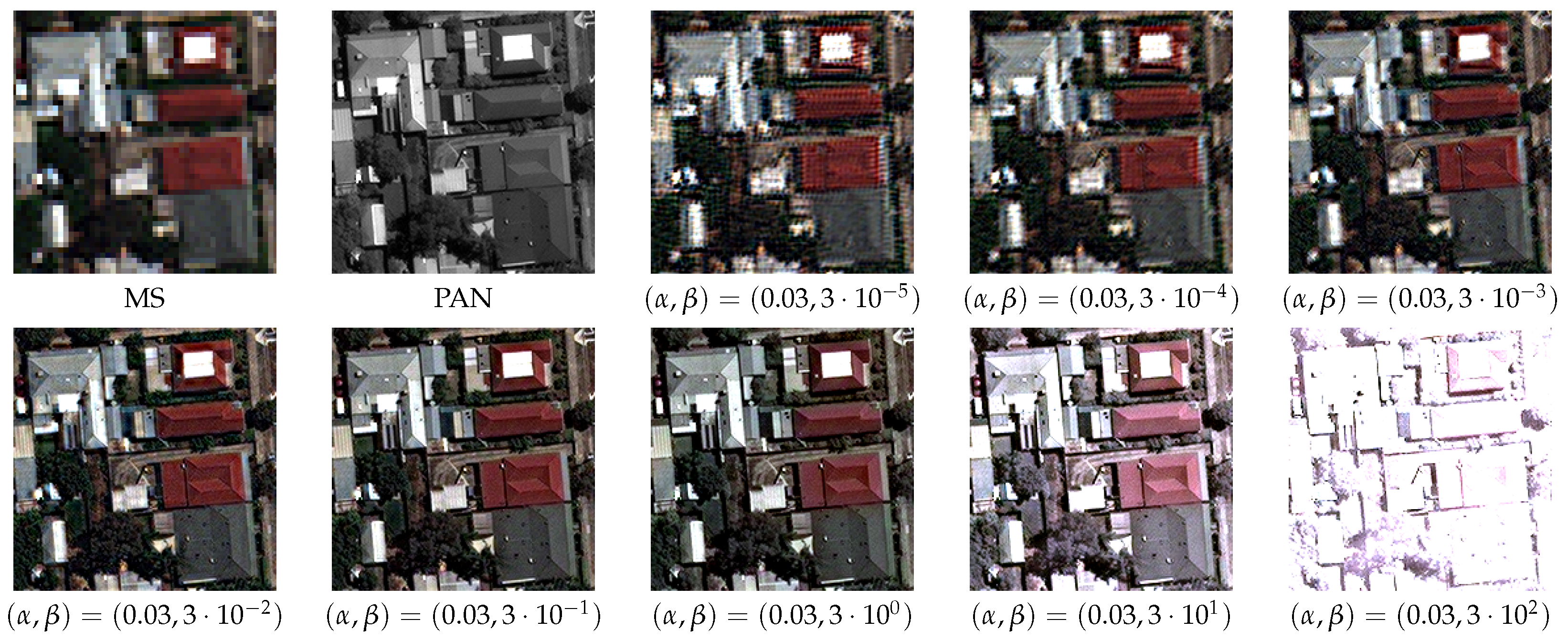
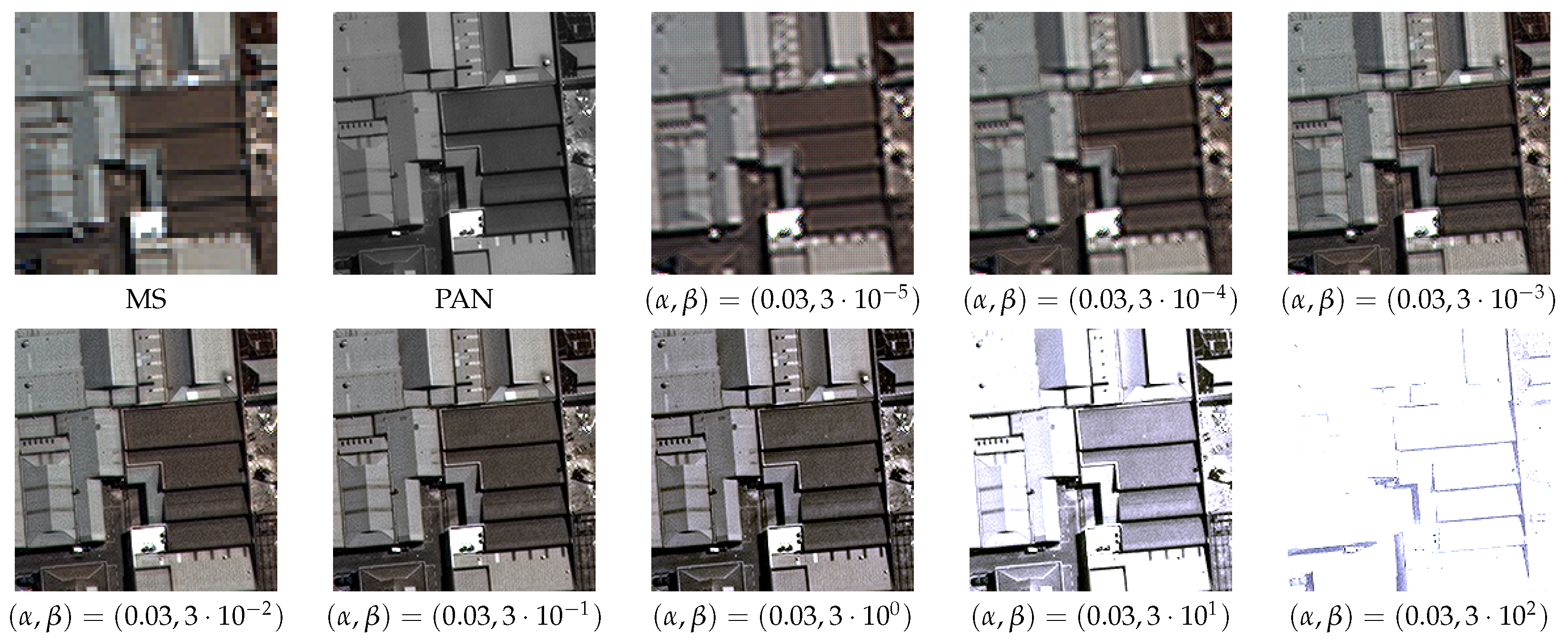
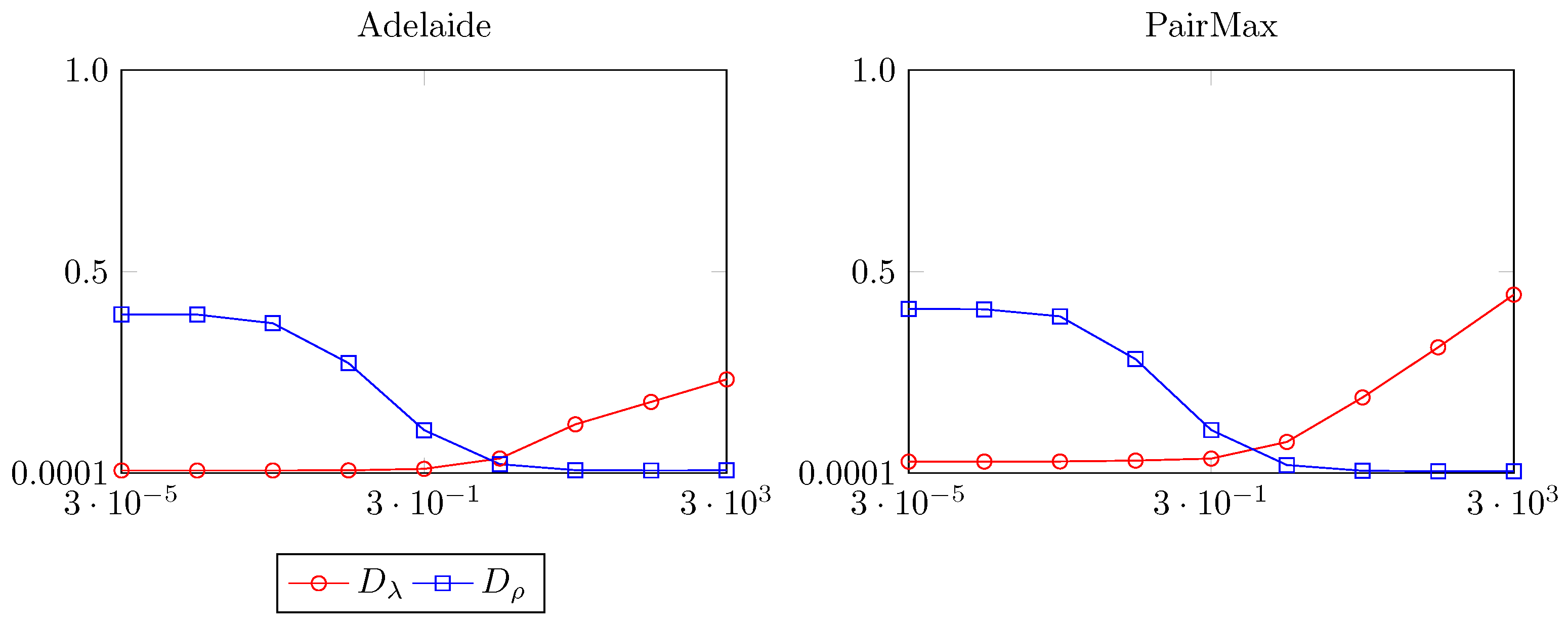
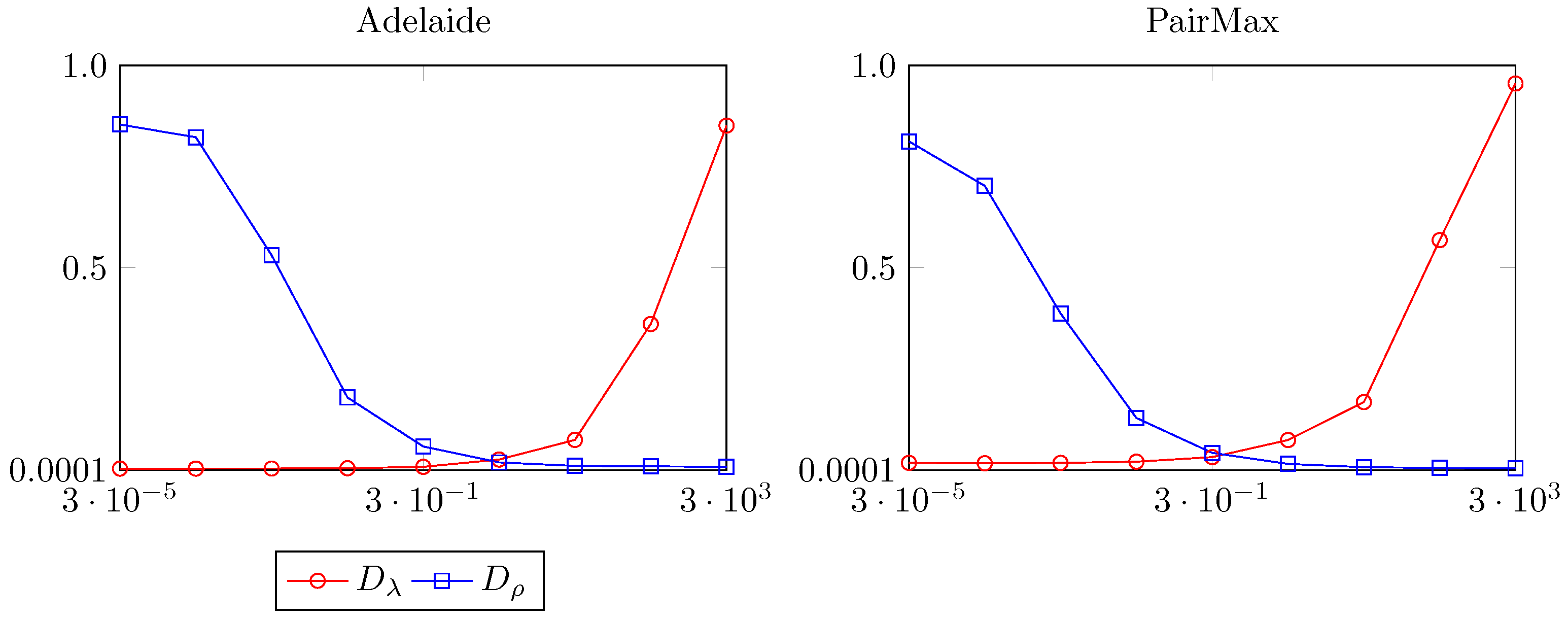
To obtain a reliable and generalizable assessment, we conducted experiments on a large and varying dataset. We used several images acquired by the WorldView-3 satellite (see

Table 3. WV3 Dataset, with number of crops for training, validation and test. Adelaide courtesy of DigitalGlobe©. Fortaleza, Mexico City, Xian (DigitalGlobe©) provided by ESA. Munich is part of PairMax dataset [65].

WorldView-3 (GSD at Nadir: 0.31 m)
Dataset	Training	Validation	Test
(PAN Size)	(512 × 512)	(512 × 512)	(2048 × 2048)
Fortaleza	32	8	-
Mexico City	32	8	-
Xian	32	8	-
Adelaide	-	24	3
Munich (PairMax)	-	-	3

), with three images exclusively for training and validation. We utilized one image for validating the “cross-scenario” generalization capability of our solution and also for testing. This image, with different weather and sunlight conditions, place, has never been used for training. Finally, the last image was exclusively used for testing. As there is no connection between this last test image and the training process, this experiment provides the most meaningful information about the effectiveness of our proposal. The given dataset volume and partition provide a good proxy for the quality assessment and, partially, also for the generalization capacity. Since our solution is based on a training and target-adaptation procedure, the only pre-processing step of our dataset is patch generation: training and validation are carried out on $512\times 512$ crops at PAN scale, while testing is performed on images of $2048\times 2048$.

To evalaute the performances of methods, trained and fine-tuned with our proposed framework, we compared them with several state-of-the-art methods. We rely on two benchmark toolboxes [1,43], which contain algorithms belonging to all four main categories recalled in Section 1: CS, MRA, VO and ML. We have exploited most of the methods provided in this collections, except few VO solutions that suffer from library incompatibilities. In addition to these, we selected five state-of-the-art unsupervised deep learning-based algorithm, retrained on our datasets to ensure a fair comparison. A summary of all comparative methods is provided in

Table 4. Detailed list of all reference methods.

Component Substitution (CS)
BT-H [3], BDSD [66], C-BDSD [67], BDSD-PC [4], GS [14], GSA [2], C-GSA [20], PRACS [68]
Multiresolution Analysis (MRA)
AWLP [5], MTF-GLP [6], MTF-GLP-FS [69], MTF-GLP-HPM [6], MTF-GLP-HPM-H [3],
MTF-GLP-HPM-R [7], MTF-GLP-CBD [70], C-MTF-GLP-CBD [20], MF [71]
Variational Optimization (VO)
FE-HPM [21], SR-D [22], TV [8]
Supervised Deep Learning-based
PNN [32], A-PNN [36], A-PNN-TA [36], BDPN [37], DiCNN [38], DRPNN [72],
FusionNet [12], MSDCNN [33], PanNet [11]
Unsupervised Deep Learning-based
QSS [45], GDD [56], PanGan [48], Z-PNN [46], $\lambda$-PNN [47]

.

It is worth underlining that assessing the performance of pansharpening algorithms is still an open problem due to the lack of ground truth. We consider full-resolution no-reference-based indexes, which separately assess spectral and spatial fidelity. Specifically, we consider the spectral distortion index ($D_{\lambda }$), proposed by Khan et al. [62], along with the reprojection indexes, R-SAM and R-ERGAS, proposed in [61] for spectral quality assessment, and the correlation distortion index, $D_{\rho }$, for spatial quality assessment.

In our experiments, we used a NVIDIA DGX Station A100, with an AMD EPYC 7742 64-Core Processor CPU, 512 GB RAM, and four NVIDIA A100-SXM4 GPUs with 40 GB of graphic memory each, produced by NVIDIA Corporation, Santa Clara (CA). USA. To assess the impact of different weightings, we pre-trained the three models using the Adam optimizer with a learning rate of $\eta =2·{10}^{-4}$ for 50 epochs.

3.2. Finding the Correct $\alpha /\beta$ Balance

We optimized the parameters $\left(\alpha ,\beta \right)$, beginning with an initial coarse search across a broad hyperparameter space, followed by a more precise refinement within the range $\left(\alpha ,\beta \right)\in \left[{10}^{-3},{10}^1\right]\times \left[{10}^{-2},{10}^2\right]$. Utilizing a logarithmic scale, we sampled 500 configurations to balance the spectral and spatial loss components during target adaptation on the validation set over 200 epochs. For each sampled configuration, we recorded, alongside the final pansharpening results, the values of the loss terms at the end of the tuning iterations. Additionally, we logged the loss values from the pre-trained model, denoted as ${\mathcal{L}}_{\lambda }^{\left(0\right)}$ and ${\mathcal{L}}_S^{\left(0\right)}$, to serve as a reference for evaluating the benefits of tuning for each component. Figure 4 and Figure 5 present the ${\mathcal{L}}_{\lambda }$ and ${\mathcal{L}}_S$ values achieved during fine-tuning for the sampled configurations $(\alpha ,\beta )$, for Z-PNN (left), PanNet (middle), and BDPN (right), for one of the Adelaide validation images. Similar results have been obtained with different validation images, which are not presented for the sake of brevity.

In this phase, we focused on generating comprehensive scatter plots to visualize the impact of various $\left(\alpha ,\beta \right)$ configurations on spectral and spatial loss components. Square (Figure 4) and circular (Figure 5) markers represent the respective loss components, with marker size corresponding to the loss values. A quantile-based color-coded clustering facilitates easier visual inspection of the scatter plots. In all scatter plots, triangular markers denote unstable configurations, attributed to spectral loss in Figure 4 spatial loss in Figure 5. Unstable configurations are classified as weakly divergent (${\mathcal{L}}_{*}^{\left(0\right)}<{\mathcal{L}}_{*}<10{\mathcal{L}}_{*}^{\left(0\right)}$) and strongly divergent (${\mathcal{L}}_{*}>10{\mathcal{L}}_{*}^{\left(0\right)}$). Two red lines delineate an ideal domain where both losses exhibit convergent behavior.

3.3. Comparative Analysis

By examining the scatter plots, we observe a transition region for all three models where the black squares change to blue ones (i.e., where the spectral loss value is close to $q_1$) in Figure 4 and where the dots change from blue to black, in Figure 5. This convergence basin defines the values of $\alpha$ and $\beta$ that optimize performance both spectrally and spatially. To maintain symmetry, we select the pair $\left(\alpha ,\beta \right)=\left(0.03,0.3\right)$ from this region as the optimal value, as it is roughly at the center of our plots. Since we are interested not only in finding the optimal value but also in studying the effects of various loss components on the final results, we have uniformly sampled 9 $\beta$ values from the horizontal line $\alpha =0.03$, comprising the optimal balance value chosen. These configurations were uniformly chosen for the Z-PNN, PanNet, and BDPN networks to establish a basis for testing proposed solutions. We increased the number of tuning iterations to 500 for these cases to achieve more precise results. With these models, we first analyzed the effects of wrong balance visually inspecting the results.

Sample results from the Adelaide test dataset for these selected $(\alpha ,\beta )$ configurations are displayed in Figure 6, Figure 7 and Figure 8. Results from the PairMax dataset, which yielded similar outcomes, are omitted for brevity.

Thus, we also deepen the correlation between the losses and the metrics used for the evaluation. We quantitatively evaluated our sampled weights using established spectral consistency indexes $D_{\lambda }$ [62], R-ERGAS and R-SAM and the spatial consistency index $D_{\rho }$ [61]. Given that the three spectral indexes provided comparable indications, we present only $D_{\lambda }$ for brevity. The experiments have been conducted on both the test sets and the values obtained are visually plotted in Figure 9, Figure 10 and Figure 11 for Z-PNN, PanNet and BDPN, respectively. The plot on the left refers to the values obtained on the three Adelaide crops, averaged for the fixed $(\alpha ,\beta )$. while on the right are displayed the averaged values of spectral consistency index $D_{\lambda }$ and the structural consistency index $D_{\rho }$ obtained on the three PairMax images.

Finally, numerical results are summarized in

Table 5. Average results on WV3-Test. Left: Adelaide. Right: Munich (PairMax). Best, Second, and Third ranked comparative algorithms are in red, blue, and green, while proposed Balanced solutions are in bold.

Method	Adelaide				PairMax
	${\mathit{D}}_{\mathit{\lambda }}$	R-SAM	R-ERGAS	${\mathit{D}}_{\mathit{\rho }}$	${\mathit{D}}_{\mathit{\lambda }}$	R-SAM	R-ERGAS	${\mathit{D}}_{\mathit{\rho }}$
EXP	0.0724	5.1446	4.6528	0.8441	0.0637	2.6788	3.9106	0.8542
BT-H	0.0652	5.1339	4.4104	0.0757	0.0793	2.9367	4.1615	0.0487
BDSD	0.0969	6.3726	5.3757	0.1219	0.1198	3.3852	5.5961	0.0749
C-BDSD	0.1198	6.6654	6.1608	0.1822	0.1370	3.9009	6.7313	0.1128
BDSD-PC	0.0802	5.7458	4.8476	0.0885	0.1075	3.3266	5.4472	0.0585
GS	0.0854	5.3908	4.8940	0.0934	0.1281	3.5500	5.0121	0.0722
GSA	0.0612	5.5015	4.4211	0.0739	0.0754	3.8093	4.4156	0.0507
C-GSA	0.0614	5.6468	4.4500	0.1299	0.0782	3.7375	4.4110	0.0603
PRACS	0.0602	5.1321	4.2519	0.1715	0.0628	2.9408	3.9187	0.1953
AWLP	0.0493	5.1313	3.9130	0.1028	0.0432	2.5507	3.0784	0.0793
MTF-GLP	0.0493	5.1570	3.9348	0.0842	0.0416	2.4502	2.9481	0.0556
MTF-GLP-FS	0.0513	5.1646	3.9989	0.1090	0.0428	2.4565	2.9792	0.0672
MTF-GLP-HPM	0.0492	5.2024	3.9451	0.0891	0.0479	2.9681	3.3831	0.0605
MTF-GLP-HPM-H	0.0488	5.2352	3.9550	0.0813	0.0425	2.5682	2.9528	0.0492
MTF-GLP-HPM-R	0.0510	5.1782	3.9988	0.1209	0.0423	2.4742	2.9861	0.0711
MTF-GLP-CBD	0.0515	5.1643	4.0069	0.1124	0.0432	2.4588	2.9950	0.0701
C-MTF-GLP-CBD	0.0565	5.1537	4.1845	0.2081	0.0468	2.6051	3.2540	0.1628
MF	0.0444	5.1306	3.7584	0.1128	0.0424	2.4981	3.0371	0.0780
FE-HPM	0.0503	5.1766	4.0367	0.1115	0.0427	2.5400	3.1030	0.0728
SR-D	0.0557	5.3438	4.2833	0.3014	0.0340	2.3290	2.7768	0.1857
TV	0.0352	4.1076	3.3427	0.2149	0.0403	1.7289	2.8877	0.1684
PNN	0.1059	7.2978	6.5981	0.4612	0.4163	8.0292	9.1146	0.4754
A-PNN	0.0598	5.2748	4.2779	0.5144	0.1693	3.5492	4.3984	0.6649
A-PNN-FT	0.0558	5.1300	4.1730	0.3087	0.0845	2.5642	3.5205	0.3352
BDPN	0.1229	5.8025	5.7712	0.1624	0.2944	6.5828	7.6926	0.3107
DiCNN	0.1207	6.4165	5.9754	0.3957	0.2169	4.9339	6.0772	0.4101
DRPNN	0.1168	5.8407	5.6579	0.1945	0.1981	4.9018	6.5979	0.1861
FusionNet	0.0730	5.4970	4.7655	0.4133	0.2382	4.5529	5.3020	0.3402
MSDCNN	0.1349	6.1317	5.8902	0.2005	0.3923	7.6591	6.6639	0.3484
PanNet	0.0554	5.0563	4.1737	0.3403	0.0609	2.5416	3.3221	0.2970
QSS	0.0590	5.2782	4.2730	0.2853	0.0828	3.1963	3.5671	0.2843
PanGan	0.6586	14.6330	13.7631	0.7134	0.3816	15.0563	17.5895	0.1317
GDD	0.1949	11.2320	7.4459	0.6440	0.3044	9.9670	8.6931	0.5867
Z-PNN	0.0374	4.8544	3.2925	0.0946	0.0919	3.5759	3.7666	0.1012
$\lambda$-PNN	0.0203	3.7631	2.5363	0.0574	0.0341	2.3690	2.6606	0.0515
Balanced Z-PNN	0.0194	3.4759	2.3798	0.1084	0.0415	2.1883	2.5103	0.1126
Balanced PanNet	0.0170	3.3167	2.2524	0.0592	0.0332	2.0381	2.4103	0.0435
Balanced BDPN	0.0412	5.3797	3.3833	0.1025	0.0934	3.3760	3.5132	0.0884

, comparing our “Balanced” solutions with other state-of-the-art methods for pansharpening on both testing datasets.

4. Discussion

To evaluate the impact of different weightings on the spectral and spatial loss components, we focus on Figure 4 and Figure 5, which respectively display the ${\mathcal{L}}_{\lambda }$ and ${\mathcal{L}}_S$ values achieved during fine-tuning by the three CNNs for the sampled $(\alpha ,\beta )$ configurations.

In this validation phase, we begin by examining the results for Z-PNN, as shown in the scatter plots on the left in both figures. As anticipated, when $\beta$ is smaller relative to $\alpha$, the spectral loss decreases (Figure 4, leftmost scatter), and vice versawhen $\beta$ increases relative to $\alpha$. These scatter plots clearly illustrate that the two loss terms present an antagonist behaviour between each other: each loss term diverges as the other approaches zero when the balance $(\alpha ,\beta )$ is outside a specific range, roughly delineated by the red pair of lines. Moreover, it is possible to identify a basin in which both loss components exhibit convergent behaviour. In this range of values, the antagonistic nature of the losses, balancing the need to preserve low frequencies while injecting more high frequencies, creates an optimal trade-off between colours and details in the final results. In this region, we have selected the parameters $\left(\alpha ,\beta \right)=\left(0.03,0.3\right)$, which reflect values close to $q_1$ for both losses. Similar observations can be extended to the other two architectures, PanNet and BDPN. Notably, deeper architectures demonstrate a broader the convergence basin for the two loss components. This suggests that deeper networks have a greater capacity to balance spectral and spatial losses effectively, with reference to their initial value ${\mathcal{L}}_{*}^{\left(0\right)}$, across a wider range of $(\alpha ,\beta )$ values.

In the testing phase, to understand the effects of this trade-off between spectral and spatial consistency on the outcome, we fine-tuned the three architectures for 500 epochs on the test dataset. Figure 6, Figure 7 and Figure 8 present sample (taken from Adelaide dataset) results obtained by Z-PNN, PanNet, and BDPN, respectively, fine-tuned with selected $(\alpha ,\beta )$ balances, ranging from spectrally boosted (high $\alpha /\beta$) to spatially boosted (low $\alpha /\beta$) settings. For all methods, higher $\alpha /\beta$ ratios produce a faithful colour response (compared to the MS) but result in poor spatial details (compared to the PAN), exhibiting blur and noisy textural patterns. Conversely, lower $\alpha /\beta$ ratios enhance the injection of PAN details into the pansharpened image, at the cost of spectral degradation (chromatic shift). Finally, a good balance guarantees precise colours and clean details, correctly injected within the scene.

In addition to visual inspection, we quantitatively evaluated how different $(\alpha ,\beta )$ configurations impact on the evaluation metrics. The values obtained are visually plotted in Figure 9, Figure 10 and Figure 11 for Z-PNN, PanNet, and BDPN, respectively. This analysis provides interesting insights: focusing on the red lines, indicating $D_{\lambda }$, at parity of $\alpha$, for high $\beta$ weights $D_{\lambda }$ diverges as expected. However, for low $\beta$ values, the spectral consistency metric remains substantially constant. Conversely, moving to the $D_{\rho }$ curve, plotted in blue, this trend becomes specular. The convergence of $D_{\lambda }$ ($D_{\rho }$) is guaranteed even with not large $\alpha /\beta$ (low $\alpha /\beta$) ratios, and the network can correctly inject details without any critical loss of colours until a specific limit configuration, the optimal configuration.

This configuration (indicated as “Balanced” version) is used for overall comparison.

Table 5 presents numerical results for both the Adelaide and Munich (PairMax) datasets. The “Balanced” configuration, for all three methods, achieves highly competitive indexes across all metrics. It is worth noting a general difficulty for BDPN in preserving colours compared to the other two CNNs, likely due to its architecture, which includes several layers for feature extraction from the P component but relatively few for processing the information from M. Nonetheless, these results remain competitive compared to many other deep-learning methods and most model-based approaches.

5. Conclusions

In this work, we demonstrate the antagonistic nature between spectral and spatial losses necessary for training deep learning-based pansharpening algorithms. Unsupervised approaches show critical sensitivity to this balance, which can lead to degraded performance in color or detail. Through extensive validation with three state-of-the-art CNNs, we empirically define a general rule for effectively balancing these losses to achieve an optimal trade-off between spectral and spatial quality. This involves identifying the optimal $\alpha /\beta$ ratio, which constrains spectral loss values while minimizing structural loss. The $\alpha$ and $\beta$ parameters are chosen based on the transition area between black and blue squares in specific figures.

We also analyze the effects of individual losses and their combinations on final results, both through visual inspection and evaluation metrics. Our balanced approach compares favorably with several state-of-the-art pansharpening methods, yielding promising results.

However, our solution has limitations: it is not suitable for optimizing adversarial losses, which must be contrastive by nature. It also does not address challenges such as moving objects or pansharpening of bands not covered by PAN wavelengths. Future improvements could involve developing a more precise formula to automatically and dynamically set the optimal balance based on image content.

References

1. Vivone, G.; Dalla Mura, M.; Garzelli, A.; Restaino, R.; Scarpa, G.; Ulfarsson, M.O.; Alparone, L.; Chanussot, J. A New Benchmark Based on Recent Advances in Multispectral Pansharpening: Revisiting Pansharpening With Classical and Emerging Pansharpening Methods. IEEE Geosci. Remote Sens. Mag. 2021, 9, 53–81. [Google Scholar] [CrossRef]
2. Aiazzi, B.; Baronti, S.; Selva, M. Improving component substitution pansharpening through multivariate regression of MS+Pan data. IEEE Trans. Geosci. Remote Sens. 2007, 45, 3230–3239. [Google Scholar] [CrossRef]
3. Lolli, S.; Alparone, L.; Garzelli, A.; Vivone, G. Haze Correction for Contrast-Based Multispectral Pansharpening. IEEE Geosci. Remote Sens. Lett. 2017, 14, 2255–2259. [Google Scholar] [CrossRef]
4. Vivone, G. Robust Band-Dependent Spatial-Detail Approaches for Panchromatic Sharpening. IEEE Trans. Geosci. Remote Sens. 2019, 57, 6421–6433. [Google Scholar] [CrossRef]
5. Otazu, X.; González-Audícana, M.; Fors, O.; Núñez, J. Introduction of sensor spectral response into image fusion methods. Application to wavelet-based methods. IEEE Trans. Geosci. Remote Sens. 2005, 43, 2376–2385. [Google Scholar] [CrossRef]
6. Alparone, L.; Garzelli, A.; Vivone, G. Intersensor Statistical Matching for Pansharpening: Theoretical Issues and Practical Solutions. IEEE Trans. Geosci. Remote Sens. 2017, 55, 4682–4695. [Google Scholar] [CrossRef]
7. Vivone, G.; Restaino, R.; Chanussot, J. A regression-based high-pass modulation pansharpening approach. IEEE Trans. Geosci. Remote Sens. 2017, 56, 984–996. [Google Scholar] [CrossRef]
8. Palsson, F.; Sveinsson, J.R.; Ulfarsson, M.O. A New Pansharpening Algorithm Based on Total Variation. IEEE Geosci. Remote Sens. Lett. 2014, 11, 318–322. [Google Scholar] [CrossRef]
9. Wang, T.; Fang, F.; Li, F.; Zhang, G. High-Quality Bayesian Pansharpening. IEEE Trans. Image Process. 2019, 28, 227–239. [Google Scholar] [CrossRef]
10. Masi, G.; Cozzolino, D.; Verdoliva, L.; Scarpa, G. CNN-based Pansharpening of Multi-Resolution Remote-Sensing Images. In Proceedings of the Joint Urban Remote Sensing Event 2017, Dubai, United Arab Emirates, 6–8 March 2017. [Google Scholar]
11. Yang, J.; Fu, X.; Hu, Y.; Huang, Y.; Ding, X.; Paisley, J. PanNet: A Deep Network Architecture for Pan-Sharpening. In Proceedings of the ICCV 2017, Venice, Italy, 22–29 October 2017. [Google Scholar] [CrossRef]
12. Deng, L.J.; Vivone, G.; Jin, C.; Chanussot, J. Detail injection-based deep convolutional neural networks for pansharpening. IEEE Trans. Geosci. Remote Sens. 2020, 59, 6995–7010. [Google Scholar] [CrossRef]
13. Chavez, P.S.; Kwarteng, A.W. Extracting spectral contrast in Landsat thematic mapper image data using selective principal component analysis. Photogramm. Eng. Remote Sens. 1989, 55, 339–348. [Google Scholar]
14. Laben, C.A.; Brower, B.V. Process for Enhancing the Spatial Resolution of Multispectral Imagery Using Pan-Sharpening. U.S. Patent 6011875, 4 January 2000. [Google Scholar]
15. Gillespie, A.R.; Kahle, A.B.; Walker, R.E. Color enhancement of highly correlated images. II. Channel ratio and “chromaticity” transformation techniques. Remote Sens. Environ. 1987, 22, 343–365. [Google Scholar] [CrossRef]
16. Tu, T.M.; Huang, P.S.; Hung, C.L.; Chang, C.P. A fast intensity hue-saturation fusion technique with spectral adjustment for IKONOS imagery. IEEE Geosci. Remote Sens. Lett. 2004, 1, 309–312. [Google Scholar] [CrossRef]
17. Ranchin, T.; Wald, L. Fusion of high spatial and spectral resolution images: The ARSIS concept and its implementation. Photogramm. Eng. Remote Sens. 2000, 66, 49–61. [Google Scholar]
18. Khan, M.M.; Chanussot, J.; Condat, L.; Montanvert, A. Indusion: Fusion of Multispectral and Panchromatic Images Using the Induction Scaling Technique. IEEE Geosci. Remote Sens. Lett. 2008, 5, 98–102. [Google Scholar] [CrossRef]
19. Aiazzi, B.; Alparone, L.; Baronti, S.; Garzelli, A. Context-driven fusion of high spatial and spectral resolution images based on oversampled multiresolution analysis. IEEE Trans. Geosci. Remote Sens. 2002, 40, 2300–2312. [Google Scholar] [CrossRef]
20. Restaino, R.; Mura, M.D.; Vivone, G.; Chanussot, J. Context-Adaptive Pansharpening Based on Image Segmentation. IEEE Trans. Geosci. Remote Sens. 2017, 55, 753–766. [Google Scholar] [CrossRef]
21. Vivone, G.; Simões, M.; Dalla Mura, M.; Restaino, R.; Bioucas-Dias, J.M.; Licciardi, G.A.; Chanussot, J. Pansharpening Based on Semiblind Deconvolution. IEEE Trans. Geosci. Remote Sens. 2015, 53, 1997–2010. [Google Scholar] [CrossRef]
22. Vicinanza, M.R.; Restaino, R.; Vivone, G.; Mura, M.D.; Chanussot, J. A Pansharpening Method Based on the Sparse Representation of Injected Details. IEEE Geosci. Remote Sens. Lett. 2015, 12, 180–184. [Google Scholar] [CrossRef]
23. Palsson, F.; Ulfarsson, M.O.; Sveinsson, J.R. Model-Based Reduced-Rank Pansharpening. IEEE Geosci. Remote Sens. Lett. 2020, 17, 656–660. [Google Scholar] [CrossRef]
24. Vitale, S.; Ferraioli, G.; Pascazio, V. A New Ratio Image Based CNN Algorithm for SAR Despeckling. In Proceedings of the IGARSS 2019, Yokohama, Japan, 28 July–2 August 2019; pp. 9494–9497. [Google Scholar] [CrossRef]
25. Fayad, I.; Ienco, D.; Baghdadi, N.; Gaetano, R.; Alvares, C.A.; Stape, J.L.; Ferraço Scolforo, H.; Le Maire, G. A CNN-based approach for the estimation of canopy heights and wood volume from GEDI waveforms. Remote Sens. Environ. 2021, 265, 112652. [Google Scholar] [CrossRef]
26. Nyborg, J.; Pelletier, C.; Lefèvre, S.; Assent, I. TimeMatch: Unsupervised cross-region adaptation by temporal shift estimation. ISPRS J. Photogramm. Remote Sens. 2022, 188, 301–313. [Google Scholar] [CrossRef]
27. Vitale, S.; Ferraioli, G.; Pascazio, V. Analysis on the Building of Training Dataset for Deep Learning SAR Despeckling. IEEE Geosci. Remote Sens. Lett. 2022, 19, 4015005. [Google Scholar] [CrossRef]
28. Haq, M.A. CNN based automated weed detection system using UAV imagery. Comput. Syst. Sci. Eng. 2022, 42, 837–849. [Google Scholar]
29. Belmouhcine, A.; Burnel, J.C.; Courtrai, L.; Pham, M.T.; Lefèvre, S. Multimodal Object Detection in Remote Sensing. In Proceedings of the IGARSS 2023—2023 IEEE International Geoscience and Remote Sensing Symposium, Pasadena, CA, USA, 16–21 July 2023; pp. 1245–1248. [Google Scholar] [CrossRef]
30. Haq, M.A.; Hassine, S.B.H.; Malebary, S.J.; Othman, H.A.; Tag-Eldin, E.M. 3D-CNNHSR: A 3-Dimensional Convolutional Neural Network for Hyperspectral Super-Resolution. Comput. Syst. Sci. Eng. 2023, 47, 2689–2705. [Google Scholar]
31. Guarino, G.; Ciotola, M.; Vivone, G.; Scarpa, G. Band-Wise Hyperspectral Image Pansharpening Using CNN Model Propagation. IEEE Trans. Geosci. Remote Sens. 2024, 62, 5500518. [Google Scholar] [CrossRef]
32. Masi, G.; Cozzolino, D.; Verdoliva, L.; Scarpa, G. Pansharpening by Convolutional Neural Networks. Remote Sens. 2016, 8, 594. [Google Scholar] [CrossRef]
33. Yuan, Q.; Wei, Y.; Meng, X.; Shen, H.; Zhang, L. A Multiscale and Multidepth Convolutional Neural Network for Remote Sensing Imagery Pan-Sharpening. IEEE J. Sel. Top. Appl. Earth Obs. Remote Sens. 2018, 11, 978–989. [Google Scholar] [CrossRef]
34. Liu, X.; Wang, Y.; Liu, Q. Psgan: A Generative Adversarial Network for Remote Sensing Image Pan-Sharpening. In Proceedings of the 2018 25th IEEE International Conference on Image Processing (ICIP), Athens, Greece, 7–10 October 2018; pp. 873–877. [Google Scholar]
35. Shao, Z.; Cai, J. Remote Sensing Image Fusion With Deep Convolutional Neural Network. IEEE J. Sel. Topics Appl. Earth Observ. 2018, 11, 1656–1669. [Google Scholar] [CrossRef]
36. Scarpa, G.; Vitale, S.; Cozzolino, D. Target-Adaptive CNN-Based Pansharpening. IEEE Trans. Geosci. Remote Sens. 2018, 56, 5443–5457. [Google Scholar] [CrossRef]
37. Zhang, Y.; Liu, C.; Sun, M.; Ou, Y. Pan-Sharpening Using an Efficient Bidirectional Pyramid Network. IEEE Trans. Geosci. Remote Sens. 2019, 57, 5549–5563. [Google Scholar] [CrossRef]
38. He, L.; Rao, Y.; Li, J.; Chanussot, J.; Plaza, A.; Zhu, J.; Li, B. Pansharpening via Detail Injection Based Convolutional Neural Networks. IEEE J. Sel. Top. Appl. Earth Obs. Remote Sens. 2019, 12, 1188–1204. [Google Scholar] [CrossRef]
39. Guarino, G.; Ciotola, M.; Vivone, G.; Poggi, G.; Scarpa, G. PCA-CNN Hybrid Approach for Hyperspectral Pansharpening. IEEE Geosci. Remote Sens. Lett. 2023, 20, 5511505. [Google Scholar] [CrossRef]
40. Gong, M.; Zhang, H.; Xu, H.; Tian, X.; Ma, J. Multipatch Progressive Pansharpening With Knowledge Distillation. IEEE Trans. Geosci. Remote Sens. 2023, 61, 5401115. [Google Scholar] [CrossRef]
41. Gong, M.; Ma, J.; Xu, H.; Tian, X.; Zhang, X.P. D2TNet: A ConvLSTM Network With Dual-Direction Transfer for Pan-Sharpening. IEEE Trans. Geosci. Remote Sens. 2022, 60, 5409114. [Google Scholar] [CrossRef]
42. Kumar, D.G.; Joseph, C.; Subbarao, M.V. An Efficient PAN-sharpening of Multispectral Images using Multi-scale Residual CNN with Sparse Representation. In Proceedings of the 2024 International Conference on Integrated Circuits and Communication Systems (ICICACS), Raichur, India, 23–24 February 2024; pp. 1–8. [Google Scholar] [CrossRef]
43. Deng, L.j.; Vivone, G.; Paoletti, M.E.; Scarpa, G.; He, J.; Zhang, Y.; Chanussot, J.; Plaza, A. Machine Learning in Pansharpening: A benchmark, from shallow to deep networks. IEEE Geosci. Remote Sens. Mag. 2022, 10, 279–315. [Google Scholar] [CrossRef]
44. Wald, L.; Ranchin, T.; Mangolini, M. Fusion of satellite images of different spatial resolution: Assessing the quality of resulting images. Photogramm. Eng. Remote Sens. 1997, 63, 691–699. [Google Scholar]
45. Luo, S.; Zhou, S.; Feng, Y.; Xie, J. Pansharpening via Unsupervised Convolutional Neural Networks. IEEE J. Sel. Top. Appl. Earth Obs. Remote Sens. 2020, 13, 4295–4310. [Google Scholar] [CrossRef]
46. Ciotola, M.; Vitale, S.; Mazza, A.; Poggi, G.; Scarpa, G. Pansharpening by Convolutional Neural Networks in the Full Resolution Framework. IEEE Trans. Geosci. Remote Sens. 2022, 60, 5408717. [Google Scholar] [CrossRef]
47. Ciotola, M.; Poggi, G.; Scarpa, G. Unsupervised Deep Learning-Based Pansharpening With Jointly Enhanced Spectral and Spatial Fidelity. IEEE Trans. Geosci. Remote Sens. 2023, 61, 5405417. [Google Scholar] [CrossRef]
48. Ma, J.; Yu, W.; Chen, C.; Liang, P.; Guo, X.; Jiang, J. Pan-GAN: An unsupervised pan-sharpening method for remote sensing image fusion. Inf. Fusion 2020, 62, 110–120. [Google Scholar] [CrossRef]
49. Zhou, H.; Liu, Q.; Wang, Y. PGMAN: An Unsupervised Generative Multiadversarial Network for Pansharpening. IEEE J. Sel. Top. Appl. Earth Obs. Remote Sens. 2021, 14, 6316–6327. [Google Scholar] [CrossRef]
50. Liu, X.; Liu, X.; Dai, H.; Kang, X.; Plaza, A.; Zu, W. Mun-GAN: A Multiscale Unsupervised Network for Remote Sensing Image Pansharpening. IEEE Trans. Geosci. Remote Sens. 2023, 61, 5404018. [Google Scholar] [CrossRef]
51. Zhou, H.; Liu, Q.; Weng, D.; Wang, Y. Unsupervised Cycle-Consistent Generative Adversarial Networks for Pan Sharpening. IEEE Trans. Geosci. Remote Sens. 2022, 60, 5408814. [Google Scholar] [CrossRef]
52. Qu, Y.; Baghbaderani, R.K.; Qi, H.; Kwan, C. Unsupervised Pansharpening Based on Self-Attention Mechanism. IEEE Trans. Geosci. Remote Sens. 2021, 59, 3192–3208. [Google Scholar] [CrossRef]
53. Ni, J.; Shao, Z.; Zhang, Z.; Hou, M.; Zhou, J.; Fang, L.; Zhang, Y. LDP-Net: An Unsupervised Pansharpening Network Based on Learnable Degradation Processes. IEEE J. Sel. Top. Appl. Earth Obs. Remote Sens. 2022, 15, 5468–5479. [Google Scholar] [CrossRef]
54. Wang, D.; Zhang, P.; Bai, Y.; Li, Y. MetaPan: Unsupervised Adaptation With Meta-Learning for Multispectral Pansharpening. IEEE Geosci. Remote Sens. Lett. 2022, 19, 5513505. [Google Scholar] [CrossRef]
55. Ciotola, M.; Scarpa, G. Fast Full-Resolution Target-Adaptive CNN-Based Pansharpening Framework. Remote Sens. 2023, 15, 319. [Google Scholar] [CrossRef]
56. Uezato, T.; Hong, D.; Yokoya, N.; He, W. Guided deep decoder: Unsupervised image pair fusion. In Proceedings of the European Conference on Computer Vision 2020, Glasgow, UK, 23–28 August 2020; Springer: Berlin/Heidelberg, Germany, 2020; pp. 87–102. [Google Scholar]
57. Xiong, Z.; Liu, N.; Wang, N.; Sun, Z.; Li, W. Unsupervised Pansharpening Method Using Residual Network With Spatial Texture Attention. IEEE Trans. Geosci. Remote Sens. 2023, 61, 5402112. [Google Scholar] [CrossRef]
58. Alparone, L.; Aiazzi, B.; Baronti, S.; Garzelli, A.; Nencini, F.; Selva, M. Multispectral and panchromatic data fusion assessment without reference. Photogramm. Eng. Remote Sens. 2008, 74, 193–200. [Google Scholar] [CrossRef]
59. Wang, Z.; Bovik, A.C. A universal image quality index. IEEE Signal Processing Letters 2002, 9, 81–84. [Google Scholar] [CrossRef]
60. Kruse, F.A.; Lefkoff, A.; Boardman, J.; Heidebrecht, K.; Shapiro, A.; Barloon, P.; Goetz, A. The spectral image processing system (SIPS)—interactive visualization and analysis of imaging spectrometer data. Remote Sens. Environ. 1993, 44, 145–163. [Google Scholar] [CrossRef]
61. Scarpa, G.; Ciotola, M. Full-Resolution Quality Assessment for Pansharpening. Remote Sens. 2022, 14, 1808. [Google Scholar] [CrossRef]
62. Khan, M.M.; Alparone, L.; Chanussot, J. Pansharpening Quality Assessment Using the Modulation Transfer Functions of Instruments. IEEE Trans. Geosci. Remote Sens. 2009, 47, 3880–3891. [Google Scholar] [CrossRef]
63. Garzelli, A.; Nencini, F. Hypercomplex Quality Assessment of Multi/Hyperspectral Images. IEEE GRSL 2009, 6, 662–665. [Google Scholar] [CrossRef]
64. Scarpa, G.; Gargiulo, M.; Mazza, A.; Gaetano, R. A CNN-Based Fusion Method for Feature Extraction from Sentinel Data. Remote Sens. 2018, 10, 236. [Google Scholar] [CrossRef]
65. Vivone, G.; Dalla Mura, M.; Garzelli, A.; Pacifici, F. A Benchmarking Protocol for Pansharpening: Dataset, Preprocessing, and Quality Assessment. IEEE J. Sel. Top. Appl. Earth Obs. Remote Sens. 2021, 14, 6102–6118. [Google Scholar] [CrossRef]
66. Garzelli, A.; Nencini, F.; Capobianco, L. Optimal MMSE pan sharpening of very high resolution multispectral images. IEEE Trans. Geosci. Remote Sens. 2008, 46, 228–236. [Google Scholar] [CrossRef]
67. Garzelli, A. Pansharpening of Multispectral Images Based on Nonlocal Parameter Optimization. IEEE Trans. Geosci. Remote Sens. 2015, 53, 2096–2107. [Google Scholar] [CrossRef]
68. Choi, J.; Yu, K.; Kim, Y. A New Adaptive Component-Substitution-Based Satellite Image Fusion by Using Partial Replacement. IEEE Trans. Geosci. Remote Sens. 2011, 49, 295–309. [Google Scholar] [CrossRef]
69. Vivone, G.; Restaino, R.; Chanussot, J. Full Scale Regression-Based Injection Coefficients for Panchromatic Sharpening. IEEE Trans. Image Process. 2018, 27, 3418–3431. [Google Scholar] [CrossRef] [PubMed]
70. Alparone, L.; Wald, L.; Chanussot, J.; Thomas, C.; Gamba, P.; Bruce, L. Comparison of pansharpening algorithms: Outcome of the 2006 GRS-S Data-Fusion Contest. IEEE Trans. Geosci. Remote Sens. 2007, 45, 3012–3021. [Google Scholar] [CrossRef]
71. Restaino, R.; Vivone, G.; Dalla Mura, M.; Chanussot, J. Fusion of Multispectral and Panchromatic Images Based on Morphological Operators. IEEE Trans. Image Process. 2016, 25, 2882–2895. [Google Scholar] [CrossRef] [PubMed]
72. Wei, Y.; Yuan, Q.; Shen, H.; Zhang, L. Boosting the Accuracy of Multispectral Image Pansharpening by Learning a Deep Residual Network. IEEE Geosci. Remote Sens. Lett. 2017, 14, 1795–1799. [Google Scholar] [CrossRef]
Figure 1. A-PNN model for Z-PNN [46].
Remotesensing 16 03014 g001
Figure 2. PanNet architecture [11].
Remotesensing 16 03014 g002
Figure 3. BDPN model [37].
Remotesensing 16 03014 g003
Figure 4. Spectral loss terms after 200 iterations for different α , β configurations.
Remotesensing 16 03014 g004
Figure 5. Spatial loss terms after 200 iterations for different α , β configurations.
Remotesensing 16 03014 g005
Figure 6. Sample results taken from WV3 Adelaide dataset: input MS and PAN followed by related pansharpenings obtained by Z-PNN through target adaptation for 500 epochs with different ( α , β ) settings.
Remotesensing 16 03014 g006
Figure 7. Sample results taken from WV3 Adelaide dataset: input MS and PAN followed by related pansharpenings obtained by PanNet through target adaptation for 500 epochs with different ( α , β ) settings.
Remotesensing 16 03014 g007
Figure 8. Sample results taken from WV3 Adelaide dataset: input MS and PAN followed by related pansharpenings obtained by BDPN through target adaptation for 500 epochs with different ( α , β ) settings.
Remotesensing 16 03014 g008
Figure 9. Full-resolution accuracy indexes for Z-PNN, with α = 0.03 and β 3 · 10 5 , 3 · 10 4 , , 3 · 10 3 .
Remotesensing 16 03014 g009
Figure 10. Full-resolution accuracy indexes for PanNet, with α = 0.03 and β 3 · 10 5 , 3 · 10 4 , , 3 · 10 3 .
Remotesensing 16 03014 g010
Figure 11. Full-resolution accuracy indexes for BDPN, with α = 0.03 and β 3 · 10 5 , 3 · 10 4 , , 3 · 10 3 .
Remotesensing 16 03014 g011