Utilizing Visible Band Vegetation Indices from Unmanned Aerial Vehicle Images for Maize Phenotyping

Abstract

Recent advancements in high-throughput phenotyping have led to the use of drones with RGB sensors for evaluating plant traits. This study explored the relationships between vegetation indices (VIs) with grain yield and morphoagronomic and physiological traits in maize genotypes. Eight maize hybrids, including those from the UENF breeding program and commercial varieties, were evaluated using a randomized block design with four replications. VIs were obtained at various stages using drones and Pix4D Mapper 4.7.5 software. Analysis revealed significant differences in morphoagronomic traits and photosynthetic capacity. At 119 days after planting (DAP), the RGB vegetation index VARI showed a significant correlation (r = 0.99) with grain yield. VARI also correlated with female flowering (r = −0.87), plant height (r = −0.79), 100-grain weight (r = −0.77), and anthocyanin concentration (r = −0.86). PCA showed a clear separation between local and commercial hybrids, explaining 46.7% of variance at 91 DAP, 52.3% at 98 DAP, 64.2% at 112 DAP, and 66.1% at 119 DAP. This study highlights the utility of VIs in maize phenotyping and genotype selection during advanced reproductive stages.

1. Introduction

In order to meet the projected demands of global population growth by 2050, agriculture faces the challenge of increasing production [1,2]. To achieve this, the annual increase in crop yield needs to be around 2.4%. However, the current rate of predicted yield growth is only 1.3%. Therefore, it is imperative to apply innovative management strategies and use advanced techniques associated with plant breeding to obtain sustainable increases in agricultural yields, guaranteeing a secure food supply for an increasingly growing population [3].

To obtain superior cultivars, phenotyping is crucial in plant breeding programs. However, in the context of maize breeding programs in Brazil, conventional methodologies to assess phenotypic characteristics are still commonly used. These conventional approaches are often inaccurate, time-consuming, inefficient, labor-intensive, and more costly. Thus, in order to efficiently assess crop phenotypic traits, it is vital to use increasingly faster, more accurate, non-destructive, and non-invasive methods (high-resolution phenotyping) [4,5,6].

In high-resolution phenotyping, unmanned aerial vehicles (UAVs), commonly known as drones, play a key supporting role. These unmanned aircraft, equipped with RGB sensors, capture high-resolution aerial images, rapidly recording information visible to the human eye in three different spectral bands. In drones, the advantages of using RGB sensors include the ability to acquire high-resolution images, enabling detailed observations of plant phenotypic traits [7]. Additionally, the captured images make it possible to analyze colors, textures, and growth patterns, contributing to the assessment of plant vigor, the mapping of agricultural areas, and important decision-making in precision agriculture. The combination of drone mobility and the accuracy of RGB sensors make them a valuable tool in high-throughput phenotyping research and practice [8,9].

The assessment of vegetation reflectance/transmittance indices is crucial for the effective implementation of high-resolution phenotyping methodologies. This allows for the fast and accurate analysis of genotypic performance associated with photosynthetic capacity, growth, and crop development. Correctly identifying remote sensing indices that best predict genotypic variability in production and choosing the ideal crop phenological stage to analyze these indices are crucial for a good correlation with productivity and optimizing the selection of the most promising genotypes. This methodology, therefore, has significant potential to accelerate the selection of elite genotypes in breeding programs and optimize the monitoring of management practices [10,11].

Visible-band vegetation indices in the red, green, and blue (RGB) region can be calculated using different combinations of these color bands, such as the Normalized Green–Red Difference Index (NGRDI). These visible-band vegetation indices can provide important information about the vegetative development and health status of plants, which may be related to plant photosynthetic capacity and productivity. In this way, the correlation between these indices and morphophysiological traits can provide valuable insights into assessing the physiological status and potential yield of the genotypes under study. In agricultural crops, this can enable the adoption of efficient targeted management practices, with high expectations of increasing yields, despite the lack of near-infrared band information [10,12,13,14].

In high-throughput phenotyping research on maize, UAVs equipped with RGB sensors have been used to assess traits such as plant height, leaf density, and canopy coverage, as well as the effects of water stress [15,16,17]. These studies aim to understand the relationship between phenotypic traits and genotype and predict crop yields. However, the main challenges for optimizing high-resolution phenotyping include standardizing data collection and processing procedures, as well as efficiently analyzing large amounts of data. Furthermore, the accurate interpretation of information related to spectral images requires considering factors such as solar radiation intensity at the time of image acquisition, vegetation heterogeneity, and variations in environmental conditions. These considerations are essential to obtaining reliable and relevant results, thus optimizing decision-making in agricultural management [9,15,16,17,18].

Recent advances in maize phenotyping have highlighted the potential of high-throughput phenotyping as a promising tool for improving crop analysis. Saravia et al. (2022) [19] highlighted the effectiveness of multispectral images from UAVs in predicting maize yield in Peru, while Li et al. (2022) [20] used UAV oblique imagery to estimate the leaf area index and plant height from 3D point clouds. These innovations underscore the potential of RGB sensor-equipped drones to enhance phenotyping accuracy and efficiency.

Despite these advances, the use of UAVs (unmanned aerial vehicles) equipped with RGB cameras in maize phenotyping remains underexplored. Comprehensive studies are needed to fully understand their applicability and effectiveness. Therefore, the main objective of this study was to evaluate the association of RGB vegetation indices with morphoagronomic and physiological traits of corn genotypes and the ideal phenological stages for their correct assessment.

The specific scientific questions we sought to address are the following: (1) Which visible-band vegetation indices best predict genotypic variability in maize yield? (2) At which phenological stages should these indices be measured for optimal yield prediction? (3) How do these indices correlate with traditional morphoagronomic and physiological traits?

2. Materials and Methods

2.1. Plant Material, Growing Conditions, and Experimental Design

Four hybrids from the maize breeding program at the State University of North Fluminense (UENF) were assessed. These included the interpopulation hybrids UENF 506-11 (H1) and UENF 506-16 (in the registration phase) (H2), suitable for grain; UENF MSV 2210 (H3), suitable for silage and green maize; and UENF MS 2208 (H4), suitable for silage. Four commercial maize hybrids were also assessed: the double hybrids BM 207 (H5) and AG 1051 (H8) and the single hybrids LG 6036 (H6) and 30F35R (H7). The experiment was conducted at the Ilha Barra do Pomba Experimental Station in Itaocara, Rio de Janeiro state, RJ (−21.64770151S, −42.06342908W) (Figure 1) [21].

The soil was fertilized and irrigated following the recommended fertilization practices for the cultivation region, and crop treatments were performed according to the guidelines for maize [22]. The experimental design consisted of completely randomized blocks with four replications. Each plot consisted of a 4 m long row, spacing of 0.70 m between rows, and 0.20 m between plants within the row, with 80 plants per plot [21]. Throughout the experimental period, photosynthetically active radiation, average temperature, average relative humidity, and total rainfall were 1423.6 ± 296.6 µmol m⁻² s⁻¹, 22.0 ± 2.9 °C, 75 ± 5.5%, and 100.8 ± 3.3 mm, respectively. The climatological values for each day after planting (DAP) can be found in Figure S1 in Supplementary Materials, obtained from the National Institute of Meteorology (INMET) website, automatic station number 604, located approximately 12.7 km from the experiment (Cambuci—RJ). To ensure the control and quality of the data, we verified the data integrity and consistency by cross-referencing with local weather stations and historical climatological data.

2.2. RGB UAV Evaluations

A DJI Mavic 2 Pro UAV (DJI, Shenzhen, China) equipped with a Hasselblad L1D-20c camera (Hasselblad Group, Göteborg, Sweden) was used to collect aerial images. The camera had a 1″ CMOS sensor and 20 MP, which generates 5472 × 3648 pixel images. The lens featured a field of view (FOV) of approximately 77°, equivalent to 35 mm; an aperture range from f/2.8 to f/11; and a shooting range from 1 m to ∞.

In compliance with Brazilian regulations for UAV use, the drone received the certificate issued by the Unmanned Aircraft System (SISANT) of the National Civil Aviation Agency (ANAC), valid for requesting flight-plan authorization through the Automated Flight Plan Registration Approval System (SARPAS) of the Airspace Control Department (DECEA). Additionally, the aircraft had up-to-date Compulsory Insurance for Aeronautical Accidents Liability of the Operator or Aerial Carrier (RETA), and the pilot was duly registered on the SARPAS website (DECEA).

The flight plan was created using the DroneDeploy platform (DroneDeploy, Inc., San Francisco, CA, USA) at a height of 80 m above ground level. The ground sample distance (GSD) obtained was 2 cm. The total area occupied by the 32 plots was 856.8 m². Frontal and lateral overlap was set at 80%, and images were captured on days 0, 19, 34, 91, 98, 112, 119, and 139 DAP. It was possible to obtain images of the entire study area in a single flight, with a flight duration of approximately 2 min and 42 s. Flights were conducted on sunny, cloudless days between 11:00 a.m. and 1:00 p.m. to minimize shading effects. Days with minimal wind were selected to avoid altering the plant canopy structure. During each flight, 17 images were recorded at a speed of approximately 5 m s⁻¹. Images were stored on Google Drive (Google LLC, Mountain View, CA, USA) and organized by each assessment day.

To enhance image coordinate accuracy, sixfive ground control points and fivesix check points were installed in the experimental area for more precise georeferencing. Point coordinates were obtained through Real Time Kinetic (RTK) survey using a CHC X91+ geodetic GNSS pair (CHCNAV, Smart Navigation and Geo-Spatial Technology Park, Shanghai, China) with millimeter accuracy. The distribution map of the study area plots, ground control points, and check points is provided in Figure 2a. Specific pictures of the ground control points are shown in Figure 2b. The mean RMS georeferencing error was 0.010 m.

Given that the aerial images were acquired under clear sky conditions, no radiometric cross-calibration correction was deemed necessary. When the coefficients of determination between the values of calibrated and uncalibrated images are considered high, the photos did not require separate color calibration [23]. Furthermore, according to Buchaillot et al. (2019) [24], applying color calibration coefficients did not improve RGB vegetation index performance.

On each assessment day, image processing was carried out using Pix4D Mapper software (Pix4D SA, Lausanne, Switzerland). Necessary interpolations were performed for 3D reconstruction based on millions of accurately modeled points, orthomosaic creation, and digital surface model generation.

Segmented orthomosaics were used to extract a set of image variables from each experimental plot at different stages of the crop cycle [(a) 0 DAP (mission 1); (b) 19 DAP (mission 2); (c) 34 DAP (mission 3); (d) 91 DAP (mission 4); (e) 98 DAP (mission 5); (f) 112 DAP (mission 6); (g) 119 DAP (mission 7); and (h) 138 DAP (mission 8)] (Figure 3) to calculate VIs. In this experiment, we did not separate crop and soil pixels; we processed the entire set, assuming that the maize canopy was dense enough to cover the soil based on the distribution between plants and rows. Image variables were calculated from the average number of pixels within the areas of interest in each plot (four plant rows per plot). red (R), green (G), and blue (B) bands (RGB color space) were extracted using the statistical zonal tool in QGIS, while hue (H); saturation (S); lightness (L) (HSL color space); intensity (I) (HSI color space); a* (a) and b* (b) (CIElab color space); and u* (u) and v* (v) (CIEluv color space) components were extracted from images using FIJI 2.9.0 (Fiji is Just ImageJ) software [25] with the Maize Scanner Breedpix 2.0 plugin (Jaume Casadesús, IRTA, Lleida, Spain). To combine these data, we used a precise georeferencing system that allowed us to align the image data with the exact locations of the field measurements. Ground control points were used to ensure spatial matching between the UAV-obtained data and field observations.

All the VIs calculated and used in this study were based on RGB image components and are described in

Table 1. Vegetation indices extracted from RGB images.

Index	Name	Description	Calculation
SCI *	Soil Color Index	Assesses soil colors in images and may provide information about soil composition and traits [26].	(R − G)/(R + G)
GLI *	Green Leaf Index	Quantifies the green light reflected by plants, indicating photosynthetic capacity and growth [27].	(2G − R − B)/(2G + R + B)
NGRDI *	Normalized Green–Red Difference Index	Compares the difference between green and red intensities in images, providing information about plant physiological status [28].	(G − R)/(G + R)
VARI *	Visible Atmospherically Resistant Index	Assesses the physiological status of vegetation and can detect plant stress [11].	(G − R)/(G + R + B)
GA **	Green Area Index	Quantifies the area of green color in an image, which may be useful for quantifying active leaf area index [24].	% of pixels in the image in the hue range (H) from 60 to 180°
GGA **	Greener Green Area Index	Similar to GA but may provide a more sensitive assessment of green areas in an image [24].	% of pixels in the image in the hue range (H) from 80 to 180°
CSI *	Crop Senescence Index	Evaluates crop senescence intensity, that is, the degradation of chlorophyll molecules in plant canopies, which may be useful in determining stress intensity and crop development stage [24].	100 × (GA − GGA)/GA

* Calculated by LibreOffice Calc. ** Calculated Using FIJI 2.9.0 software with the Maize Scanner Breedpix 2.0 plugin. R = Red; G = Green; and B = Blue in the RGB color space.

.

2.3. Assessment of the Photosynthetic Capacity of Plants, Water Balance, and Leaf Pigments

Simultaneously conducted 98 (mission 5), 112 (mission 6), and 129 (mission 7) DAP, assessments of physiological traits (photosynthetic pigments, Normalized Difference Vegetation Index—NDVI, fluorescence emission of chlorophyll, and leaf spectroscopy) were carried out on individual plant leaves in the two central blocks (blocks 2 and 3) (Figure 4), with four plants per treatment, on the middle part of the first leaf above the ear, between 11:00 a.m. and 1:00 p.m.

The Dualex^® portable meter (FORCE-A, Orsay, France) was used to obtain relative levels of leaf chlorophyll (Chl), flavonoids (Flavs), anthocyanins (Anths), and nitrogen balance indices (NBIs) (

Table 2. Variables assessed using the portable chlorophyll and leaf pigment meter Dualex^® (FORCE-A, Orsay, France).

Variable	Name	Description
Chl	Chlorophyll	Estimate of leaf chlorophyll concentration: an indicator of photosynthetic capacity and stress [29].
Flav	Flavonoids	Estimate of leaf flavonoid concentration: associated with organic compound concentration with antioxidant functions and may play an important role in the response to environmental stress [29].
Anth	Anthocyanins	Estimate of anthocyanin concentration in plants: these pigments exhibit antioxidant properties against excessive solar radiation [29].
NBI	Nitrogen Balance Index	Associated with leaf nitrogen content and indicates leaf photosynthetic capacity [29].

). Dualex determines the chlorophyll content of a leaf based on the transmittance at two specific wavelengths. One wavelength is in the far-red region, which is absorbed by chlorophyll, while the other is in the near-infrared region, serving as a reference. Dualex measures flavonols and anthocyanins by different light wavelengths to excite the chlorophyll—green light for anthocyanins and UV light for flavanols. The NBI^® (Nitrogen Balance Index) combines chlorophyll and flavonols; it is a plant nitrogen status indicator directly correlated with massic nitrogen content.

A FieldScout CM 1000 portable NDVI meter (Spectrum Technologies, Aurora, IL, USA) was used to obtain the Normalized Difference Vegetation Index (NDVI) [28]. To perform this assessment, the NDVI meter was maintained 0.5 m from the plants, and readings were taken between 11:00 a.m. and 1:00 p.m. (UTC-3).

The fluorescence emission of chlorophyll, on the same leaves used to assess leaf pigments, was measured from 11:00 a.m. to 1:00 p.m. using the non-modulated Pocket PEA fluorimeter (Hansatech Instruments, King’s Lynn, UK), and the variables φPo, φEo, φDo, ABS/CSo e Piabs were obtained (

Table 3. Variables evaluated using the non-modulated Pocket PEA fluorimeter (Hansatech Instruments, UK).

Variable	Name	Description
φPo = TRo/ABS	Quantum yield	Efficiency with which PSII converts photons from photosynthetically active radiation (PAR) absorbed in active photochemistry of photosystem II (PSII) by reducing QA (Quinone Acceptor). It assesses the rate of using PAR for the production of chemical energy [30]
φEo = ETo/ABS	Quantum yield of electron transfer	Throughout the electron transport chain, this variable estimates the efficiency with which absorbed PAR photons and electrons from QA- are used to promote the movement of electrons beyond QA [30].
φDo = DIo/ABS	Quantum efficiency of energy dissipation	Efficiency with which PSII regulates the dissipation of light energy when the demand for chemical energy for photosynthesis is lower. Excess light energy is dissipated as heat instead of being used in photosynthesis, preventing the formation of reactive oxygen species [30].
ABS/Cso	Number of antenna complexes	Quantifies the number of light-harvesting (antenna) complexes relative to the number of open reaction centers ready for active photochemistry [30].
PIabs	Performance Index for absorption	An indicator of the functional activity of PSII normalized to the absorbed energy [30].

). Before fluorescence emission assessments, an area in the middle of the leaf was selected, and leaf clips provided by the fluorimeter manufacturer were used to keep a 6 mm² sampled area in the dark for 30 min to ensure the entire photochemical system remained oxidized. Additionally, the CI710 leaf spectrometer (CiD BioScience, Camas, WA, USA) to simultaneously measure the transmission, absorption and reflection of light over a wide range of wavelengths covering visible and near-infrared (NIR) light, in the wavelength range of 360–1100 nm. For this research, the following indices from the adaxial part of individual leaves were used: ARI1, ARI2, CRI1, CRI2, SIPI, FRI, CNDVI, Ge, NDVIe, NPCI, SRPI, PRI, PSRI, and WBI (

Table 4. Variables evaluated using the CI710 leaf spectrometer (CiD BioScience, USA).

Variable	Name	Description	Calculation
CRI1	Chlorophyll Reflectance Index 1	Associated with the total chlorophyll content of the leaves [31].	(1/W 510) − (1/W 550)
CRI2	Chlorophyll Reflectance Index 2	Similar to CRI1, associated with the total chlorophyll content of the leaves [31].	(1/W 510) − (1/W 700)
SIPI	Structure-Independent Pigmentation Index	Provides information on pigment concentrations in plants, independent of leaf structure [32].	(W 800 − W 445)/(W 800 + W 680)
FRI	Flavonoids Reflectance Index	Detects flavonoids in plants, responsible for yellow and red colors [29].	(1/W 410 − 1/W 460) × W 800
CNDVI	Cumulative Normalized Difference Vegetation Index	A normalized version of NDVI considering the influence of canopy geometry on measurement [33].	(W 750 − W 705)/(W 750 + W 705)
Ge	Green Band Index	Associated with the total chlorophyll content of the leaves [11].	W 554/W 677
NDVI2	Normalized Difference Vegetation Index	Associated with the total chlorophyll content of the leaves [28].	(W 800 − W 680)/(W 800 + W 680)
SRPI	Simple Ratio Pigment Index	Associated with the carotenoids/chlorophyll ratio in leaves [34].	W 430/W 680
PRI	Photochemical Reflectance Index	Associated with the epoxidation state of xanthophylls, indicating the efficiency of photosynthetic radiation use [35].	(W 531 − W 570)/(W 531 + W 570)
PSRI	Senescence Reflectance Index	Associated with the senescence process of leaves, evaluating the intensity of the carotenoid/chlorophyll ratio [36].	(W 680 − W 500)/W 750
WBI	Water Band Index	Evaluates leaf water status [35].	W 900/W 970

Wavelength (W).

). To that end, the same leaves selected to assess leaf pigment levels and chlorophyll fluorescence emission were used, and assessments were conducted between 11:00 a.m. and 1:00 p.m. (UTC-3).

Using the selected variables, we aimed to characterize the overall absorption, capture, transport, and dissipation of energy in the photosynthetic apparatus. Measurements by device took an average of five minutes to be carried out in each plot. To complete the one-day survey, it took approximately two hours per device.

2.4. Assessment of Morphoagronomic Traits

Male (MM) and female flowering (FF) were expressed in number of DAP until 50% of the plants in the study area of each plot showed emerged panicles and style-stigmas, respectively. Average plant height (AP) was expressed in meters (m), measured from the ground to the node of panicle insertion. The AP was measured at 80 days after planting, when plant growth ceases after flowering and the plants start to fill the grains. Before harvest, the total number of plants (NP) was determined by counting the total number of plants in the plot and the number of ears (NES) by counting the number of ears per plot. The average ear length (AEL) and average ear diameter (AED) were determined using a digital caliper and expressed in millimeters (mm), obtained by the average of six ears. The 100-grain weight (100 GW) was obtained by weighing 100 grains from each row of the plot, on an analytical balance with a resolution of 0.001 g. Grain yield (GY) was evaluated after threshing the ears, estimated in kg per plot, corrected for 13% moisture, and converted to kg/ha⁻¹ [21].

2.5. Statistical Analysis

Boxplots (Figure S2) were used to evaluate the variability of the data and identify outliers. The data underwent an analysis of variance of mean squares using the F-test to compare the means of different experimental groups (maize genotypes) and determine if there are statistically significant differences between them. The null hypothesis (H0) was that the means are equal, while the alternative hypothesis (H1) was that at least one mean was different. We reject H0 if the p-value is less than 0.05. Next, variables with significant results were submitted to Pearson’s correlation analysis to measure the strength and direction of the linear association between pairs of traits. Tukey’s test was used as post-hoc analysis following ANOVA to perform comparisons between genotype means and identify which genotypes differ significantly at the 5% probability level.

Principal component analysis (PCA) was used to reduce the dimensionality of the data and identify patterns in the measured variables, as well as identify the principal components that explain most of the variation. Statistical analyses were performed using Genes version 1990.2023.45 [37] software, and graphs and PCAs were processed in the R program. Individual analysis was conducted to assess the difference between genotypes according to the following statistical model:

$$Yij=\mu +Blj+Gi+ϵij$$

(1)

where Yij is the observed value for the variable under study referring to the combination of the i-th level of the Genotype factor with the j-th level of the Crop Year factor; μ is the overall mean; Blj is the effect of the j-th block, assuming NID (0, σ²); Gi is the effect of the i-th level of the Genotype factor on the observed value; ϵij is the experimental error associated with the observation, assuming NID (0, σ²).

3. Results

3.1. Orthomosaics

To obtain drone data, each flyover date during the experiment (mission) produced 17 image files, which formed orthomosaic products (a single image for each mission in tif format). The image processing reports produced by Pix4D Mapper indicate that all quality characteristics were achieved. These report parameters are associated with images (median of key points per image), the dataset (calibrated and enabled images), optimal camera use (internal camera parameters), and georeferencing (3D control points on the ground and root-mean-square error (RMS)).

The orthomosaics resulting from processing had a spatial resolution of 2 cm/pixel and are shown in Figure 5, with the plot division vector (in white) (block and hybrid).

The first planting of the commercial hybrid BM 207 (H5) at 0 DAP was unsuccessful (Figure 5b), so this hybrid was replanted at 19 DAP, and because it was at a different phenological stage to the other hybrids, it was not considered in any statistical analysis. To arrive at this split, the analysis of variance of the mean squares was carried out using the f-test and Pearson’s correlation analysis, considering all the hybrids. As all the RGB VANT variables did not show significant correlations with grain yield (GY), we opted to disregard hybrid 5. Figure 5d shows damage to the plants of hybrids 5, 8, 6, and 2 in block 4. However, data from block 4 were collected and included in the statistical analyses. Leaf senescence was observed from 112 DAP (Figure 5f–h).

3.2. Mean Square Variance Using the F-Test

In the analysis of variance, significant differences were observed for all morpho-agronomic variables, except for the number of plants (NP). Among the variables associated with photosynthetic capacity and pigments, only φEo and PIabs (98 DAP), ABS/Cso and PIabs (112 DAP), and Anth (119 DAP) showed significant results. Finally, starting from the evaluation at 91 DAP, the RGB components and indices showed significant differences for most characteristics, with exceptions being 91 DAP (a, u, v, GA, GGA, and CSI), 98 DAP (L and v), 112 and 119 DAP (I, L, b, and v). The missions prior to 91 DAP (missions 1, 2, and 3) did not show significant differences for the indices and were not used in the analyses (

Table 5. Analysis of mean square variance in random blocks of RGB components and RGB vegetation (UAV).

GL	Treat.	Me.	CV%	Treat.	Me.	CV%	Treat.	Me.	CV%
Var.	34 DAP			91 DAP			98 DAP
SCI	0.0010 ns	−0.07	34.76	0.0011 **	−0.12	5.34	0.0016 **	−0.08	10.74
GLI	0.0008 ns	0.17	12.35	0.0015 **	0.16	5.32	0.0010 **	0.12	7.06
NGRDI	0.0010 ns	0.07	34.76	0.0011 **	0.12	5.34	0.0016 **	0.08	10.74
VARI	0.0019 ns	0.10	34.75	0.0024 **	0.19	5.59	0.0046 **	0.14	11.88
I	0.0001 ns	0.17	6.11	0.0005 **	0.14	7.80	0.0003 *	0.13	7.25
H	45.5221 ns	77.18	6.90	68.8384 **	98.78	2.69	214.0860 **	92.6	5.22
S	0.0009 ns	0.31	6.07	0.0033 **	0.19	10.78	0.0023 *	0.16	14.80
L	2.0473 ns	20.49	5.55	8.3870 *	16.25	10.01	3.9758 ns	15.2	9.50
a	2.4035 ns	−8.24	12.29	1.1599 ns	−8.29	8.51	1.0117 *	−6.42	7.89
b	1.4848 ns	16.52	5.22	257.7162 **	13.95	35.76	119.3165 *	11.56	49.67
u	2.2366 ns	−2.88	36.41	0.3437 ns	−4.04	12.44	0.6857 **	−2.65	11.25
v	1.5307 ns	14.39	6.00	4.9469 ns	9.32	15.7	2.0049 ns	7.86	16.71
GA	0.0030 ns	0.37	10.61	0.0000 ns	0.45	0.93	0.0002 ns	0.44	2.68
GGA	0.0071 ns	0.21	30.98	0.0009 ns	0.43	5.07	0.0093 **	0.36	11.97
CSI	274.9316 ns	44.89	28.78	48.3089 ns	4.61	93.26	382.7851 **	18.99	44.75
	112 DAP			119 DAP
SCI	0.0026 **	−0.03	40.86	0.0034 **	−0.01	269.95
GLI	0.0010 **	0.09	14.85	0.0014 **	0.07	21.78
NGRDI	0.0026 **	0.03	40.86	0.0034 **	0.01	269.95
VARI	0.0071 **	0.06	41.24	0.0091 **	0.01	258.08
I	0.0001 ns	0.15	8.25	0.0000 ns	0.16	5.60
H	459.5754 **	74.60	7.970	691.5479 **	62.53	10.76
S	0.0026 **	0.18	12.59	0.0019 *	0.18	13.11
L	10,364,503 ns	625.65	514.58	0.3807 ns	17.74	6.21
a	3.3344 **	−4.96	15.51	6.4594 **	−3.66	19.87
b	2.7117 ns	10.43	13.64	1.6698 ns	10.19	9.69
u	3.6427 **	−1.20	45.86	6.3041 **	−0.01	4968.95
v	1.5572 ns	8.84	17.32	1.0389 ns	8.62	10.61
GA	0.0166 **	0.34	11.08	0.0379 **	0.24	19.90
GGA	0.0518 **	0.17	33.20	0.0334 **	0.10	40.55
CSI	2143.4674 **	56.10	18.69	1482.5698 **	66.23	11.99

ns—non-significant using the F-test; ** and * significant at 1 and 5% probability; respectively; according to the F-test. Treatments (Treat.); Mean (Me.); Coefficient of variation (CV%); Variables (Var.); Days after Planting (DAP); Soil Color Index (SCI); Green Leaf Index (GLI); Normalized Green Red Difference Index (NGRDI); Visible Atmospheric Resistance Index (VARI); Intensity (I); Hue (H); Saturation (S); Lightness (L); a* (a); b* (b); u* (u); v* (v); Green Area Index (GA); Greener Area Index (GGA); Crop Senescence Index (CSI).

,

Table 6. Analysis of variance of mean squares, in random blocks, of the morphoagronomic traits assessed.

Variables	Treatments	Mean	CV (%)
MF	37.5804 **	60.45	2.41
FF	37.5751 **	64.18	3.09
AP	0.2265 **	2.66	2.65
NP	73.4048 ns	79.39	8.64
AEL	780.6262 **	248.42	1.92
AED	17.0620 **	59.00	2.13
NE	380.7381 **	66.61	12.52
100 GW	1184.0254 **	32.71	4.74
GY	7,991,551.6579 **	6400.66	15.31

ns—non-significant using the F-test; ** significant at 1% probability; respectively, using the F-test. Coefficient of Variation (CV%); male flowering (MF); female flowering (FF); average plant height (AP); number of plants (NP); average ear length (AEL); average ear diameter (AED); number of ears (NE); 100-grain weight (100 GW); grain yield (GY) [21].

and

Table 7. Analysis of variance of mean squares, in random blocks, of the traits assessed and associated with photosynthetic capacity, water status and pigment concentration.

GL	Treat.	Me.	CV%	Treat.	Me.	CV%	Treat.	Me.	CV%
Var.	98 DAP			112 DAP			119 DAP
Dualex® (FORCE-A, Orsay, France)
Chl	10.8994 ns	40.38	6.20	21.1315 ns	34.58	13.66	32.8303 ns	31.67	15.85
Flav	0.0438 ns	1.30	10.33	0.0467 ns	1.38	11.00	0.0442 ns	1.39	9.26
Anth	0.0005 ns	0.17	8.64	0.0006 ns	0.22	11.88	0.0032 **	0.22	6.35
NBI	29.9538 ns	32.72	11.39	36.3143 ns	26.32	19.95	11.7909 ns	23.23	14.92
FieldScout CM 1000 (Spectrum Technologies, Aurora, IL, USA)
NDVI	0.0113 ns	0.71	9.24	0.0138 ns	0.66	16.85	0.0131 ns	0.63	11.09
Pocket PEA (Hansatech Instruments, UK)
φPo	0.0028 ns	0.72	4.40	0.0012 ns	0.75	2.43	0.0031 ns	0.73	6.04
φEo	0.0049 *	0.45	7.08	0.0026 ns	0.45	6.61	0.0024 ns	0.40	12.61
φDo	0.0028 ns	0.28	11.24	0.0012 ns	0.25	7.36	0.0031 ns	0.27	16.16
ABS/Cso	406,779 ns	4464.43	7.67	159,096 *	4305.82	3.35	384,162 ns	4148.59	13.56
PIabs	1.7304 **	2.68	12.78	2.4285 **	2.85	17.50	0.5089 ns	1.95	34.43
CI710 (CiD BioScience, USA)
ARI1	0.0000 ns	−0.02	25.30	0.0000 ns	−0.01	24.09	0.0001 ns	−0.01	94.89
ARI2	0.0183 ns	−0.91	22.45	0.0151 ns	−0.66	23.54	0.1613 ns	−0.41	96.35
CRI1	0.0000 ns	0.03	13.39	0.0000 ns	0.05	11.16	0.0000 ns	0.03	28.57
CRI2	0.0000 ns	0.01	33.33	0.0000 ns	0.03	19.81	0.0000 ns	0.02	32.53
SIPI	0.0007 ns	0.74	3.20	0.0004 ns	0.76	2.55	0.0051 ns	0.67	12.23
FRI	0.0121 ns	1.07	17.24	0.0196 ns	1.12	18.33	0.0641 ns	1.14	19.35
CNDVI	0.0018 ns	0.52	7.58	0.0009 ns	0.49	11.00	0.0094 ns	0.37	35.16
Ge	0.0441 ns	2.03	5.05	0.0452 ns	2.24	5.46	0.2413 ns	1.97	19.57
NDVIe	0.0010 ns	0.73	4.05	0.0005 ns	0.75	3.00	0.0227 ns	0.61	25.14
NPCI	0.0002 ns	0.10	18.27	0.0002 ns	0.09	14.97	0.0207 ns	0.16	78.28
SRPI	0.0005 ns	0.82	3.56	0.0005 ns	0.84	2.60	0.0274 ns	0.76	19.93
PRI	0.0002 ns	0.04	31.41	0.0001 ns	0.02	63.65	0.0007 ns	0.01	275.91
PSRI	0.0000 ns	−0.03	14.34	0.0000 *	−0.02	16.58	0.0158 ns	0.02	446.00
WBI	0.0007 ns	0.72	5.57	0.0018 ns	0.96	5.33	0.0005 ns	0.74	10.35

Non-significant (ns); by the F test; ** and * significant at 1 and 5% probability; respectively; by the F test. Treatments (Treat.); Mean (Me.); Coefficient of Variation (CV%); Variables (Var.); Days After Planting (DAP). Chlorophyll (Chl); Flavonoids (Flavs); Anthocyanins (Anths); Nitrogen Balance Index (NBI); Normalized Difference Vegetation Index (NDVI); Effective quantum yield of photosystem II, PSII (φPo); Quantum yield of excess thermal energy dissipation (φEo); Quantum yield of regulatory dissipation (φDo); Number of light-harvesting complexes per open reaction center (ABS/Cso); Probability of an antenna complex being excited (PIabs); Anthocyanin Reflectance Index 1 (ARI1); Anthocyanin Reflectance Index 2 (ARI2); Chlorophyll Reflectance Index 1 (CRI1); Chlorophyll Reflectance Index 2 (CRI2); Structure-Independent Pigmentation Index (SIPI); Flavonoid Reflectance Index (FRI); Cumulative Normalized Difference Vegetation Index (CNDVI); Green Band measured by the spectrometer (Ge); Normalized Difference Vegetation Index measured by the spectrometer (ENDVI); Normalized Pigment Chlorophyll Index (NPCI); Simple Ratio Pigment Index (SRPI); Photochemical Reflectance Index (PRI); Plant Senescence Reflectance Index (PSRI); Water Band Index (WBI).

).

3.3. Pearson’s Correlation

After analyzing the ANOVA information, variables with significant differences were submitted to Pearson’s correlation analysis. The results of morphoagronomic variables versus UAV RGB variables and indices are shown in

Table 8. Phenotypic correlation between morphoagronomic variables and UAV RGB variables and indices.

Variables	MF	FF	AP	AEL	AED	NE	100 GW	GY
91 DAP
SCI	0.49	0.82 *	0.52	0.65	−0.82 *	−0.47	0.31	−0.57
GLI	−0.10	−0.45	−0.16	−0.53	0.54	0.18	0.08	0.10
NGRDI	−0.49	−0.82 *	−0.52	−0.65	0.82 *	0.47	−0.31	0.57
VARI	−0.61	−0.91 **	−0.62	−0.63	0.86 *	0.57	−0.45	0.73
I	0.66	0.83 *	0.71	0.61	−0.87 *	−0.39	0.42	−0.68
H	−0.79 *	−0.86 *	−0.72	−0.34	0.68	0.64	−0.76 *	0.97 **
S	0.39	0.13	0.30	−0.22	0.04	−0.21	0.52	−0.48
L	0.73	0.84 *	0.76 *	0.57	−0.86 *	−0.40	0.49	−0.75
b	−0.29	−0.51	−0.23	−0.52	0.70	−0.01	0.15	0.22
98 DAP
SCI	0.59	0.87 *	0.62	0.39	−0.84 *	−0.73	0.52	−0.87 *
GLI	−0.30	−0.68	−0.37	−0.48	0.74	0.49	−0.16	0.48
NGRDI	−0.59	−0.87 *	−0.62	−0.39	0.84 *	0.73	−0.52	0.87 *
VARI	−0.61	−0.87 *	−0.64	−0.34	0.81 *	0.76 *	−0.58	0.91 **
I	0.57	0.83 *	−0.66	0.48	−0.84 *	−0.62	0.46	−0.73
H	−0.65	−0.79 *	−0.64	−0.19	0.67	0.76 *	−0.69	0.96 **
S	0.47	0.28	0.39	−0.18	−0.10	−0.36	0.60	−0.61
a	0.36	0.72	0.40	0.39	−0.73	−0.61	0.28	−0.63
b	−0.29	−0.50	−0.23	−0.53	0.69	−0.03	0.16	0.20
u	0.56	0.84 *	0.56	0.35	−0.78 *	−0.72	0.51	−0.87 *
GGA	−0.66	−0.89 **	−0.75	−0.43	0.79 *	0.78 *	−0.69	0.95 **
CSI	0.71	0.92 **	0.76 *	0.45	−0.82 *	−0.74	0.68	−0.95 **
112 DAP
SCI	0.69	0.87 *	0.79 *	0.45	−0.74	−0.73	0.75	−0.98 * *
GLI	−0.58	−0.89 **	−0.70	−0.59	0.86 *	0.67	−0.53	0.82 *
NGRDI	−0.69	−0.87 *	−0.79 *	−0.45	0.74	0.73	−0.75	0.99 **
VARI	−0.68	−0.86 *	−0.78 *	−0.42	0.72	0.74	−0.76 *	0.99 **
H	−0.67	−0.81 *	−0.78 *	−0.38	0.64	0.73	−0.80 *	0.98 **
S	0.43	0.29	0.44	−0.06	−0.07	−0.38	0.65	−0.64
a	0.65	0.89 **	0.78 *	0.54	−0.79 *	−0.72	0.69	−0.95 **
u	0.69	0.86 *	0.81 *	0.48	−0.73	−0.71	0.76 *	−0.99 **
GA	−0.65	−0.86 *	−0.87 *	−0.61	0.67	0.73	−0.84 *	0.95 **
GGA	−0.72	−0.82 *	−0.78 *	−0.38	0.69	0.66	−0.75	0.99 **
CSI	0.73	0.81 *	0.79 *	0.38	−0.69	−0.62	0.75	−0.99 **
119 DAP
SCI	0.73	0.88 *	0.79 *	0.43	−0.73	−0.72	0.77 *	−0.99 **
GLI	−0.69	−0.94 **	−0.77 *	−0.55	0.84 *	0.72	−0.66	0.92 **
NGRDI	−0.73	−0.88 *	−0.79 *	−0.43	0.73	0.72	−0.77 *	0.99 **
VARI	−0.72	−0.87 *	−0.79 *	−0.41	0.72	0.73	−0.77 *	0.99 **
H	−0.71	−0.85 *	−0.78 *	−0.39	0.68	0.73	−0.79 *	0.99 **
S	0.45	0.30	0.45	−0.06	−0.11	−0.36	0.63	−0.66
a	0.73	0.92 **	0.80 *	0.49	−0.79 *	−0.72	0.74	−0.98 **
u	0.72	0.87 *	0.80 *	0.43	−0.72	−0.72	0.78 *	−0.99 **
GA	−0.75	−0.89 **	−0.82 *	−0.48	0.75	0.68	−0.77 *	0.99 **
GGA	−0.69	−0.78 *	−0.73	−0.26	0.65	0.70	−0.74	0.98 **
CSI	0.68	0.74	0.78 *	0.28	−0.63	−0.64	0.75	−0.97 **

** and * significant at 1 and 5% probability; respectively; by phenotypic correlation. Days After Planting (DAP). Soil Color Index (SCI); Green Leaf Index (GLI); Normalized Red–Green Difference Index (NGRDI); Visible Atmospheric Resistance Index (VARI); Intensity (I); Hue (H); Saturation (S); Brightness (L); a* (a); b* (b); u* (u); v* (v); Green Area Index (GA); Greener Green Area Index (GGA); Crop Senescence Index (CSI); Male flowering (MF); Female flowering (FF); Average plant height (AP); Average ear length (AEL); Average ear diameter (AED); Number of ears (NE); 100-grain weight (100 GW); Grain yield (GY).

.

The best phenotypic correlations between morphoagronomic variables and RGB UAV variables and indices were at 91 DAP (days after planting): between MF and H (−0.79), FF and VARI (−0.91), AP and L (0.76), AED and I (0.87), 100 GW and H (−0.76), and GY and H (0.97). At 98 DAP, they were FF and CSI (0.92), AP and CSI (0.76), AED and I (−0.84), NE and GGA (0.78), and GY and H (0.96). At 112 DAP: FF and a (0.89), AP and GA (−0.78), AED and GLI (0.86), 100 GW and GA (−0.837), and GY and GGA (0.99). At 119 DAP, they were FF and GLI (−0.93), AP and GA (−0.82), AED and GLI (0.84), 100 GW and H (−0.79), and GY and NGRDI (0.99).

The phenotypic correlation between variables associated with photosynthetic capacity and leaf pigment concentration versus UAV RGB variables and indices are presented in

Table 9. Phenotypic correlation between phenotypic variables and UAV RGB variables and indices.

Variables	98 DAP		112 DAP			119 DAP
	Pocket		Pocket		CI710	Dualex
	φEo	PIabs	ABS/Cso	PIabs	PSRI	Anth
SCI	0.44	0.48	−0.11	−0.18	−0.28	0.86 *
GLI	−0.21	−0.28
NGRDI	−0.45	−0.48	0.11	0.18	0.28	−0.85 *
VARI	−0.48	−0.51	0.09	0.18	0.26	−0.86 *
I	0.55	0.51
H	−0.54	−0.54	0.03	0.22	0.24	−0.88 **
S	0.60	0.34	0.20	−0.25	0.28	0.83 *
a	0.08	0.24	−0.16	−0.31	−0.49	0.78 *
b						0.55
u	−0.35	0.34	−0.09	−0.31	−0.32	0.87 *
v						0.32
GA			−0.02	0.32	0.41	−0.83 *
GGA	−0.45	−0.46	0.08	0.20	0.15	−0.90 **
CSI	0.45	0.46	−0.10	−0.20	−0.11	0.88 **

** and * significant at 1 and 5% probability; respectively; by phenotypic correlation; blank cell represents a component or UAV RGB vegetation index with no significant difference (ANOVA) considering two repetitions for a given DAP. Days After Planting (DAP). Soil Color Index (SCI); Green Leaf Index (GLI); Normalized Green–Red Difference Index (NGRDI); Visible Atmospheric Resistance Index (VARI); Intensity (I); Hue (H); Saturation (S); Brightness (L); a (a); b (b); u* (u); v* (v); Green Area Index (GA); Greener Area Index (GGA); Crop Senescence Index (CSI); Quantum Efficiency of Thermal Energy Dissipation (φEo); Number of Light-Harvesting Complexes per Open Reaction Center (ABS/Cso); Probability of an antenna complex being excited (PIabs); Plant Senescence Reflectance Index (PSRI); Anthocyanins (Anths).

, which shows that only anthocyanin (Anth) was significantly correlated with UAV RGB variables and indices at 119 DAP, with GGA being the best correlation (−0.90).

3.4. Tukey’s Test for Pairwise Mean Comparisons

For UAV RGB variables and indices, the result of the comparative mean test (Tukey) is shown in

Table 10. Tukey’s test for pairwise mean comparison for UAV RGB vegetation indices and variables.

Variables	UENF 506-11 (H1)	UENF 506-16 (H2)	UENF MSV 2210 (H3)	UENF MS 2208 (H4)	LG 6036 (H6)	30F35R (H7)	AG 1051 (H8)
91 DAP
SCI	−0.107 a	−0.126 b	−0.108 a	−0.111 a	−0.153 c	−0.129 b	−0.109 a
GLI	0.152 bcd	0.169 b	0.148 cd	0.160 bc	0.198 a	0.151 bcd	0.138 d
NGRDI	0.107 c	0.126 b	0.108 c	0.111 c	0.153 a	0.129 b	0.109 c
VARI	0.170 d	0.198 bc	0.173 d	0.173 d	0.235 a	0.214 ab	0.180 cd
I	0.141 ab	0.138 ab	0.140 ab	0.155 a	0.118 b	0.131 ab	0.143 ab
H	94.816 c	97.950 bc	96.729 bc	94.310 c	100.438 abc	106.175 a	101.066 ab
S	0.191 ab	0.201 a	0.180 ab	0.208 a	0.225 a	0.148 b	0.152 b
L	16.500 ab	16.479 ab	16.312 ab	18.759 a	14.094 b	15.053 ab	16.543 ab
b	11.141 b	11.606 b	10.699 b	12.774 b	31.982 a	9.439 b	9.982 b
98 DAP
SCI	−0.070 a	−0.078 a	−0.067 a	−0.073 a	−0.111 b	−0.115 b	−0.075 a
GLI	0.116 bc	0.125 bc	0.110 c	0.124 bc	0.155 a	0.132 b	0.109 c
NGRDI	0.070 b	0.078 b	0.067 b	0.073 b	0.111 a	0.115 a	0.075 b
VARI	0.113 b	0.125 b	0.109 b	0.117 b	0.175 a	0.196 a	0.125 b
I	0.137 ab	0.134 ab	0.137 ab	0.143 a	0.121 b	0.124 ab	0.141 a
H	87.518 b	89.211 b	87.634 b	87.475 b	95.674 b	107.536 a	93.185 b
S	0.171 ab	0.177 ab	0.161 ab	0.185 a	0.192 a	0.125 b	0.142 ab
a	−6.018 a	−6.312 ab	−5.841 a	−6.524 ab	−7.222 b	−6.921 ab	−6.097 ab
b	9.743 b	9.901 b	9.430 b	10.729 ab	23.818 a	8.216 b	9.060 b
u	−2.275 a	−2.484 ab	−2.213 a	−2.559 ab	−3.134 bc	−3.298 c	−2.563 ab
GGA	0.329 b	0.348 ab	0.318 b	0.312 b	0.406 ab	0.441 a	0.350 ab
CSI	25.554 ab	21.003 abc	26.262 ab	29.015 a	8.464 bc	2.799 c	19.837 abc
112 DAP
SCI	−0.018 ab	−0.026 abc	−0.010 a	−0.012 ab	−0.056 cd	−0.077 d	−0.044 bc
GLI	0.083 bc	0.091 abc	0.077 c	0.081 bc	0.119 a	0.111 ab	0.087 bc
NGRDI	0.018 cd	0.026 bcd	0.010 d	0.012 cd	0.056 ab	0.077 a	0.044 bc
VARI	0.029 cd	0.041 bcd	0.016 d	0.019 d	0.088 ab	0.129 a	0.074 bc
H	67.657 bc	70.780 bc	64.515 c	64.906 c	79.859 ab	93.698 a	80.806 ab
S	0.189 abc	0.192 abc	0.188 abc	0.195 ab	0.205 a	0.141 c	0.145 bc
a	−4.343 ab	−4.713 abc	−3.948 a	−4.242 a	−6.056 bc	−6.295 c	−5.157 abc
u	−0.559 ab	−0.867 abc	−0.216 a	−0.322 a	−1.998 cd	−2.730 d	−1.676 bcd
GA	0.305 cd	0.343 bcd	0.269 d	0.277 d	0.398 ab	0.437 a	0.384 abc
GGA	0.095 b	0.105 b	0.070 b	0.056 b	0.236 a	0.358 a	0.244 a
CSI	69.431 a	69.954 a	74.004 a	80.415 a	42.097 b	18.310 b	38.505 b
119 DAP
SCI	0.015 ab	0.003 abc	0.018 a	0.025 a	−0.027 cd	−0.056 d	−0.017 bc
GLI	0.056 b	0.067 ab	0.053 b	0.050 b	0.092 a	0.096 a	0.066 ab
NGRDI	−0.015 cd	−0.003 bcd	−0.018 d	−0.025 d	0.027 ab	0.056 a	0.017 bc
VARI	−0.024 cd	−0.005 bcd	−0.029 d	−0.040 d	0.041 ab	0.094 a	0.028 bc
H	53.517 cd	58.724 bcd	51.981 d	48.982 d	69.662 b	86.139 a	68.738 bc
S	0.183 a	0.190 a	0.183 a	0.189 a	0.196 a	0.143 a	0.145 a
a	−2.763 a	−3.387 ab	−2.614 a	−2.297 a	−4.898 bc	−5.719 c	−3.955 ab
u	0.840 ab	0.348 abc	1.020 a	1.316 a	−0.884 cd	−2.187 d	−0.544 bc
GA	0.175 c	0.217 bc	0.164 c	0.136 c	0.322 ab	0.401 a	0.294 ab
GGA	0.049 cd	0.046 cd	0.034 d	0.017 d	0.136 bc	0.273 a	0.146 b
CSI	72.874 ab	79.830 a	79.566 a	86.985 a	59.168 bc	32.122 d	53.080 c

Means followed by the same letters in the row do not differ statistically at 5% probability according to Tukey’s test. From left to right: H1, H2, H3, H4 (UENF), H6, H7, and H8 (commercial). Days After Planting (DAP). Soil Color Index (SCI); Green Leaf Index (GLI); Normalized Green–Red Difference Index (NGRDI); Visible Atmospheric Resistance Index (VARI); Intensity (I); Hue (H); Saturation (S); Luminosity (L); a* (a); b* (b); u* (u); v* (v); Green Area Index (GA); Greener Green Area Index (GGA); Crop Senescence Index (CSI).

.

Table 11. Tukey’s test for pairwise mean comparison for morphoagronomic variables.

Variables	UENF 506-11 (H1)	UENF 506-16 (H2)	UENF MSV 2210 (H3)	UENF MS 2208 (H4)	LG 6036 (H6)	30F35R (H7)	AG 1051 (H8)
MF	64.625 a	61.813 ab	58.625 bc	64.250 a	57.688 c	57.688 c	58.438 bc
FF	68.000 a	64.188 abc	65.125 ab	67.500 a	60.000 c	60.688 bc	63.750 abc
AP	2.597 bc	2.614 b	2.936 a	3.062 a	2.486 bc	2.450 c	2.511 bc
AEL	250.844 bc	234.075 d	265.264 a	264.765 a	230.795 d	253.343 b	239.845 cd
AED	57.128 c	57.527 c	59.150 bc	57.172 c	62.645 a	60.771 ab	58.641 bc
NE	67.500 ab	71.500 ab	52.250 b	62.500 b	67.500 ab	83.750 a	61.250 b
100 GW	32.799 ab	31.425 ab	34.826 a	34.968 a	32.946 ab	30.461 b	31.521 ab
GY	5451.812 bc	5675.158 bc	5420.424 bc	4899.531 c	7456.675 ab	8795.251 a	7105.768 abc

Same letters in the row do not differ statistically at 5% probability according to Tukey’s test. From left to right: H1, H2, H3, H4 (local), H6, H7, and H8 (commercial). Male flowering (MF); female flowering (FF); average plant height (AP); total number of plants (NP); average ear length (AEL); average ear diameter (AED); number of ears (NE); 100-grain weight (100 GW); grain yield GY) [21].

contains the results of morphoagronomic variables. In both tables, the means and the letters indicating statistically similar groups are presented for each variable on each DAP.

With respect to morphoagronomic variables and grain yield (GY), commercial hybrid H7 (30F35R) performed best, followed by H6 (LG 6036) and H8 (AG 1051), which obtained statistically similar results. Among the local hybrids (UENF), H2 (UENF 506-16) had the highest grain yield, followed by H1 (UENF 506-11) and H3 (UENF MSV 2210). These hybrids showed similar clustering. Finally, the hybrid with the lowest average production and statistically different from the others was local hybrid H4 (UENF MS 2208).

Data from 91 DAP for RGB vegetation variables showed that local hybrids UENF MSV 2210, UENF MS 2208, and UENF 506-11 were similar in the SCI, GLI, NGRDI, and VARI variables. On the other hand, commercial hybrid LG 6036 obtained a higher average and significant differences from the others for the GLI and NGRDI variables. At 98 DAP, and compared to the commercial hybrids (H6, H7, and H8), the local hybrids (H1, H2, H3, and H4) were significantly different (Table 11). In relation to the SCI, local hybrids exhibited similar performance, while H6 and H7 were significantly different, especially H6. For the GLI variable, H6 displayed superior performance, while local hybrids exhibited lower values and more similar results. The NGRDI demonstrated that local hybrids and the commercial H8 had similar responses with the best values, while commercial H6 and H7 had lower performance. In terms of the VARI, and in relation to local hybrids, H6 and H7 showed a distinct response.

With respect to data at 112 DAP, for the SCI variable, H3 obtained a higher value, followed by hybrids H4, H2, and H1 (local), with a similar response. However, when compared to local hybrids, commercial hybrids H6, H7, and H8 showed superior performance. In relation to the GLI variable and local hybrids, once again, H6 and H7 demonstrated superior performance, with H6 obtaining the highest average. In the NGRDI, hybrids displayed a similar pattern. For this variable, and in relation to local hybrids, H7 and hybrid H8 (commercial) showed significant differences. In the VARI, H7 stood out, while local hybrids showed inferior performance and a similar response. For GGA, assessed at 112 DAP, commercial hybrids were superior to their local counterparts and exhibited the highest percentage of pixels in the green spectrum.

At 119 DAP, in the SCI variable, the performance of local hybrids H1, H2, H3, and H4 was similar and superior to that of the other hybrids. However, for the same variable, commercial hybrids H6, H7, and H8 showed significant differences. In regard to the GLI, H6 and H7 stood out with superior performance compared to local hybrids. In the NGRDI and VARI indices, hybrids displayed similar patterns, highlighting the superior performance of H7, while local hybrids demonstrated inferior and similar responses.

3.5. Principal Components

Principal component analysis (PCA) is shown in Figure 6, revealing clustering and plot dispersion in different local and commercial hybrids in multidimensional feature spaces.

The graphs of principal component analysis (PCA) conducted on different days after planting (DAP) (91, 98, 112, and 119) provide information about the response of variables and indices assessed in local and commercial hybrids. At 91 DAP, point distribution shows a separation between the local and commercial hybrid clusters, with PC1 and PC2 explaining 46.7 and 18.5% of variance, respectively. The variables SCI, AEL, I, FF, L, MF, and 100 GW contributed significantly to this difference. At 98 DAP, point dispersion decreased, with PC1 and PC2 explaining 52.3 and 14.5% of variance, respectively. GLI, I, 100 GW, MF, CSI, AP, FF, SCI, and AEL were the main variables influencing this separation. At 112 and 119 DAP, the separation became more evident, with less dispersed and closer variables, and PC1 explaining 64.2 and 66.1% of variance, respectively. During these times (112 and 119 DAP), GLI, AED, NE, GGA, GA, H, VARI, GY, and NGRDI contributed to the difference between clusters.

4. Discussion

4.1. Orthomosaic Analysis

In the present study, drone flights were conducted to collect data to assess variables of interest in a field experiment with seven maize hybrids. The results provide valuable information on the performance of these hybrids and the use of remote sensing technologies in the phenotypic assessment of this important Brazilian agribusiness crop [38,39].

The Pix4D Mapper image processing reports indicated that the image quality parameters, such as dataset, camera optimization, and georeferencing, were suitable. This suggests that the images collected at 80 m altitude during survey missions were successfully processed, resulting in high-quality orthomosaics (2 cm/pixel), which served as a basis for subsequent analyses [40].

4.2. Analysis of Variance of Mean Squares Using the F-Test

Analysis of variance revealed significant differences for most morphoagronomic and some physiological variables. All the morphoagronomic variables, except the number of plants (NP), showed significant differences among maize hybrids.

Significant differences in morphoagronomic variables among maize hybrids underscored their genetic variability, even under uniform growing conditions. This demonstrates the importance of selecting hybrids that suit specific growing conditions. These differences allow for the selection of hybrids that better meet local needs and conditions [9,41].

The number of plants (NP) showed no significant differences among hybrids, despite variations in other variables. This suggests that, under the growing conditions of the present study, all hybrids maintained a similar population density pattern. This is important for the consistency and reliability of the study results, since uniform population density among hybrids reduces potential sources of variation that could mask the effects of genetic traits on other variables under analysis [42].

Several variables related to photosynthetic capacity and pigment concentration in individual leaves showed significant differences among maize hybrids at different development stages, indicating variations in photochemical efficiency, photosynthetic pigment concentration or plant vigor. The variables φEo and PIabs at 98 DAP suggest variations in photochemical efficiency, indicating hybrid adaptations to more efficient use of photosynthetically active radiation (PAR). At 112 DAP, the variables ABS/Cso, PIabs, and PSRI, and at 119 DAP, Anth, reflect differences in leaf pigment concentration and potentially the ability to protect against environmental stresses at the time of assessments. These findings are consistent with previous studies, highlighting the importance of photosynthetic capacity and pigment concentration associated with photosynthesis and leaf protection in selecting maize hybrids suitable for specific growing conditions [43].

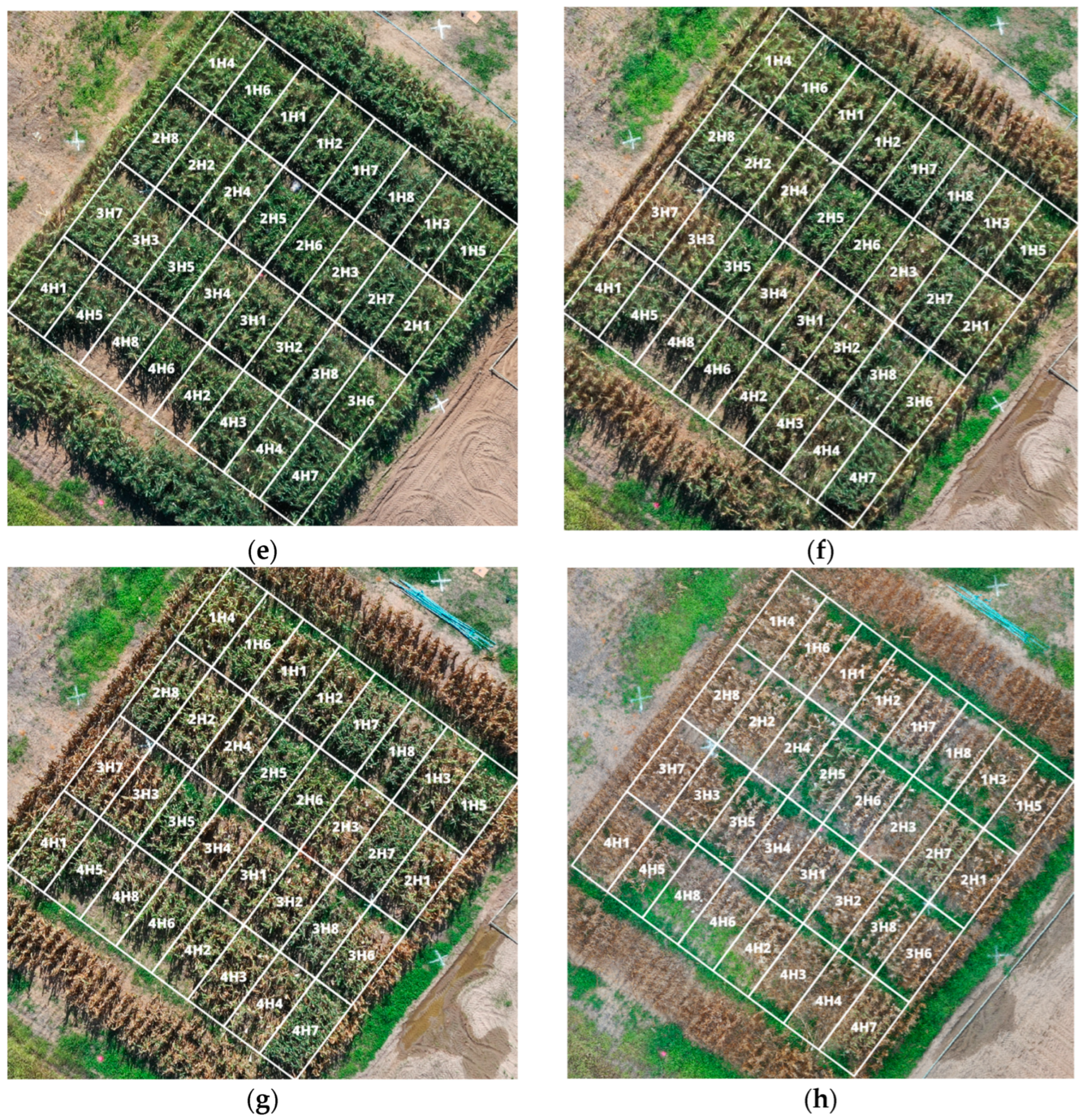
The UAV RGB (red, green, blue) indices played a significant role in differentiating between maize hybrids. These indices are sensitive to plant traits other than mineral nutrition and water availability, including leaf pigment concentration, organ structure, and overall plant vigor. The ANOVA results revealed significant differences in the RGB components across different color spaces among maize hybrids. These variations can be interpreted in terms of pigment concentration and plant structure. RGB components, representing the intensity of red, green, and blue, respectively, can provide information about plant pigment concentration and distribution [44]. For example, differences in the red spectrum may indicate variations in chlorophyll concentration, a crucial pigment for photosynthesis. The green spectrum is related to the amount of green mass in plants, while the blue spectrum reflects canopy density and plant structure [45,46]. Thus, the differences in RGB components may be associated with variations in leaf pigment concentration, photosynthetic efficiency, canopy growth, and plant development.

Vegetation indices calculated from drone images also showed significant differences among maize hybrids at different development stages. In summary, differences in RGB components across different color spaces and VIs among maize hybrids can be explained in terms of pigment concentration, photosynthetic efficiency, canopy growth, and plant vigor. These results underscore the importance of considering multiple variables and indices when assessing crop performance, given that each can provide specific information about relevant aspects of plant production.

Across different DAP, analysis of variance revealed significant variations in several components and UAV RGB indices. At the early stage (91 DAP), statistically significant differences were observed in components such as SCI, GLI, NGRDI, VARI, and I. These variations can be attributed to the initial plant response to environmental and growth factors. As the crop progressed to 98 DAP, H and S also showed significant differences, indicating possible changes in leaf structure and pigment concentration during this period. At 112 DAP, in addition to previous components, L, a, and b also exhibited significant differences, suggesting a complex evolution in plant color and structure traits. As the crop reached 119 DAP, components u and v displayed significant differences, suggesting possible variations in plant color distribution. Vegetation indices GA, GGA, and CSI also exhibited statistically significant variations across different DAPs, reflecting changes in photosynthetic efficiency and overall plant vigor as the crop cycle progressed. These results highlight the dynamics of plant traits throughout the growth cycle and the importance of considering these changes when assessing the performance of maize hybrids at different development stages [47].

4.3. Pearson Correlation Analysis

After ANOVA, variables with statistically significant differences were submitted to phenotypic correlation. At different stages of crop development, the results highlighted important correlations between morphoagronomic variables and UAV RGB indices. At 91 DAP, a strong positive correlation was observed between grain yield (GY) and component H (r = 0.97), suggesting a possible relationship between production and pixel hue [48].

In the early stage at 91 DAP, significant correlations were observed between morphoagronomic variables such as grain yield (GY) and average plant height (AP), with UAV RGB components such as GLI and VARI providing crucial information. The strong positive correlation between GY and the H index suggests that crop development at this stage is related to the amount of green mass [48]. These findings can be explained by the fact that, at this moment, the plants are in active growth, and photosynthetic efficiency, as well as pigment distribution, plays a crucial role in biomass accumulation [5].

As the crop advanced to 98 DAP, important correlations were observed, such as the strong association between GY and the CSI. This suggests that, at this stage, crop yield is closely related to leaf pigment concentration. Additionally, significant correlations between CSI and AP indicate that leaf pigment concentration and photosynthetic capacity can influence plant morphology. These associations can be explained by the fact that, at this stage, plants are reaching maximum growth and photosynthetic capacity, and differences in morphoagronomic traits and leaf pigment concentration can affect yields.

At 112 DAP, correlations between morphoagronomic variables and components and UAV RGB indices also provide important information. The strong correlation between GY and UAV RGB variables (NGRDI, VARI, u, GGA, and CSI), with a value of |0.99|, suggests that crop yield may also be related to plant photosynthetic efficiency during the critical phase of maize development, specifically during the grain-filling phase. Furthermore, the correlation between AP and the GA index indicates the importance of leaf chlorophyll concentration for plant morphology and average plant height. At this stage, chlorophyll molecule concentration plays an essential role in yield.

Vegetation indices (VIs) derived from RGB images, such as the Normalized Green–Red Difference Index (NGRDI), serve as indirect indicators of leaf density and distribution, correlating with chlorophyll content in the leaves. Chlorophyll, being a key pigment for photosynthesis, indicates the plant’s photosynthetic capacity. Therefore, higher VIs suggest greater chlorophyll levels and photosynthetic potential. However, while VIs provide an indirect estimate of chlorophyll, they do not measure it directly. The prediction of crop yield using VIs is based on their correlation with agronomic parameters like leaf area, chlorophyll content, and plant biomass, all of which influence yield. Monitoring these parameters through the growth cycle helps identify patterns indicating yield potential.

As plants reach 119 DAP, correlations continue to provide valuable data. The strong correlation (r = |0.99|) between GY and UAV variables (SCI, NGRDI, VARI, H, u, and GA) suggests that yield is related to the color distribution of plant leaves. The negative correlation between AP and the GA index indicates that average plant height may be influenced by the percentage of pixels with the H value in the green range. These associations underscore the complexity of interactions between morphoagronomic traits, leaf pigment concentration, and plant structure in the late growth cycle.

It is important to note that the relationship between photosynthetic capacity and the bands used in each index is complex. In general, the use of different colored bands (red, green, blue) to calculate UAV RGB indices is directly associated with the absorption and reflectance of chlorophyll/carotenoids, canopy density, plant morphology, and the amount of non-photosynthetic pigments present in the leaves. For example, the VARI, which uses red, green, and blue bands, is sensitive to leaf chloroplast pigment concentration and can reflect differences in chlorophyll and carotenoid concentration, essential in the photochemical phase of photosynthesis. A strong correlation was observed between grain yield (GY) and the VARI at 98 DAP (r = 0.91), 112 DAP and 119 DAP (r = 0.99). This correlation indicates a strong and significant association between this vegetation index and crop yield [47].

Among other morphoagronomic variables analyzed at different maize development stages, several exhibited significant correlations with UAV RGB indices. At 91 DAP, female flowering (FF) revealed a strong correlation (r = −0.91) with the VARI, suggesting the influence of leaf photosynthetic pigments in the early stages of the crop. In addition, at 91 DAP, average plant height (AP) showed a strong correlation (r = 0.76) with the L index, related to plant morphology, indicating that morphoagronomic traits are highly relevant in the early stages of maize growth. Additionally, other variables such as average ear diameter (AED), number of ears (NE), and 100-grain weight (100 GW) also showed significant correlations with several UAV RGB indices, including SCI, GLI, NGRDI, GA, and CSI. The ir values for these correlations varied, underscoring the complex relationships between plant morphology and the traits obtained from drone images, ranging from 0.73 to 0.88.

In regard to variables associated with photosynthetic capacity and leaf pigments, the only significant correlation observed was between Anth at 119 DAP and UAV RGB indices. This result demonstrates a notable association between Anth and remote sensing indices. The best correlation (r = −0.90) was observed with the GGA index. This implies that variations in the Anth concentration of maize leaves are strongly related to variations in the GGA index, which represents green traits in drone images. This strong correlation suggests that the amount of Anth pigment influences the quantity and distribution of green mass in maize plants, which, in turn, affects the reflectance of green captured by drone sensors. This relationship is important because it may indicate that the concentration of this pigment in maize leaves is strongly linked to vigor, photosynthetic efficiency, and response to variability in this species. Thus, drone images and UAV RGB indices are promising tools for assessing not only leaf pigment concentration but also the photosynthetic capacity and vigor of maize plants in the field. This information can be crucial for improving agronomic management and selecting genotypes with desirable leaf pigment concentration and plant vigor traits [49].

4.4. Analysis of Tukey’s Test for Pairwise Mean Comparison

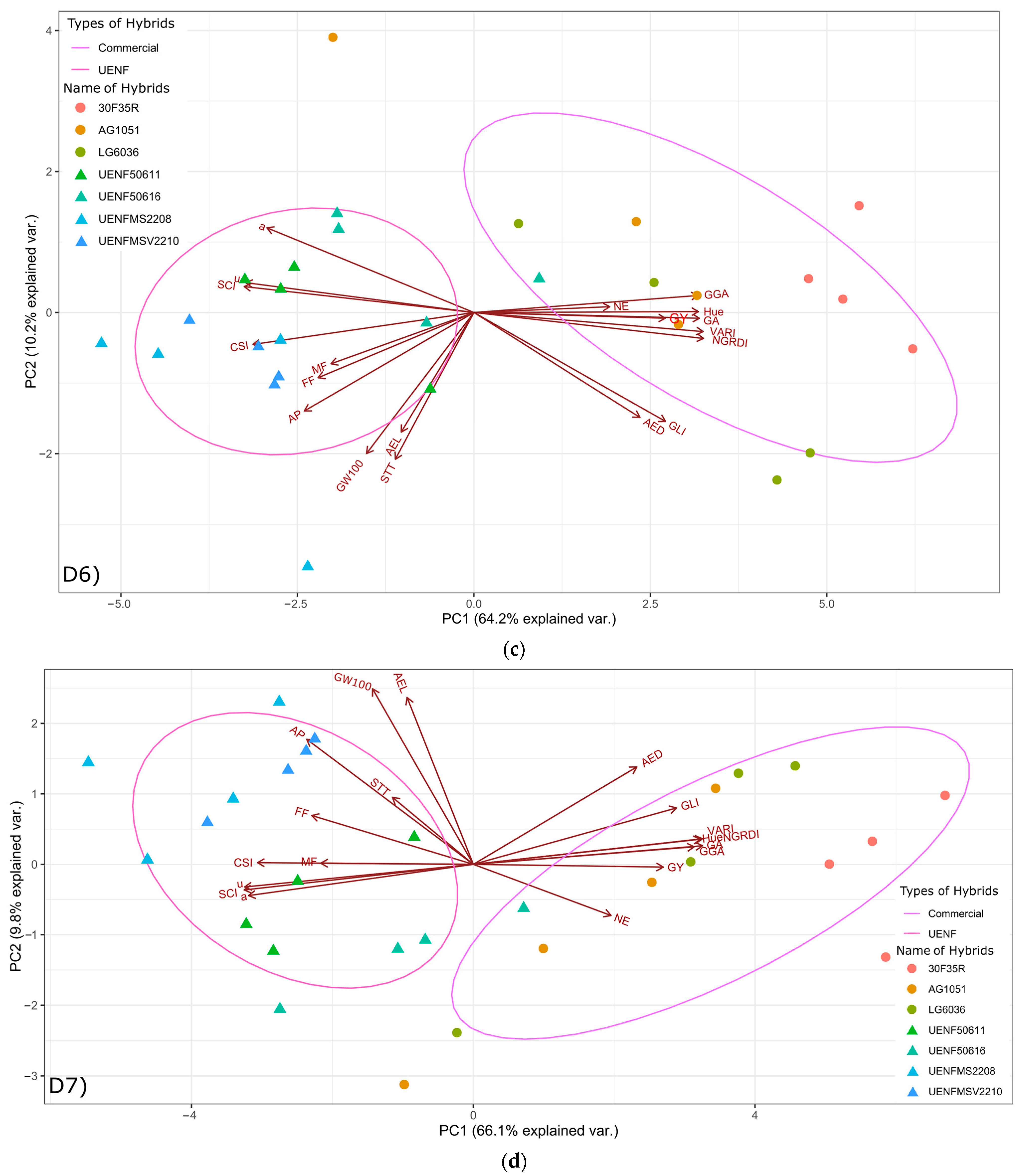
Our analysis of the Tukey’s test results revealed important information about the performance of local and commercial hybrids at different stages of crop development, especially indices that showed a strong correlation with grain yield. For example, at 112 and 119 DAP, the VARI, when compared to commercial hybrids (H6, H7, and H8), showed similar and inferior responses for local hybrids (H1, H2, H3, and H4). Hybrid H7 obtained the highest VARI value, indicating a strong association with yield. With respect to indices such as GLI, NGRDI at 112 DAP and 119 DAP, commercial hybrids (H7 and H8) demonstrated superior performance, suggesting a potential advantage in later development stages, given the positive correlation between these indices and grain yield. The SCI showed a strong negative correlation with grain yield and generally exhibited inverse clustering compared to other indices. When assessing the performance of different hybrids associated with indices related differently to agricultural yield, according to the DAP, it is essential to consider the importance of different crop development stages in the assessment.

Hybrid 30F35R (H7) showed the highest grain yield, exceeding all local hybrids. This difference is associated with the fact that the commercial hybrid is a simple variety, resulting from the crossing of two inbred lines, while local hybrids originate from interpopulation crosses. In this case, while simple hybrids capitalize on 100% of heterosis and are more uniform, interpopulation hybrids partially capture heterosis and obtain lower yields [50].

At 119 DAP and with respect to the SCI (Soil Color Index), commercial hybrids H6, H7, and H8 showed significantly lower values when compared to their local counterparts, indicating a possible difference in the average RGB values of hybrid plots. Hybrid H7 had the highest GLI (Green Leaf Index) value, suggesting a larger number of green leaves on the plants. This difference may be related to a larger photosynthetic area, since more chlorophyll can result in higher photosynthetic carbon assimilation. H7 also showed the highest NGRDI value, indicating a greater difference between green and red bands. This may be related to leaf pigment concentration, and chlorophyll concentration (since chlorophyll molecules absorb light in the electromagnetic spectrum of red and blue, and different concentrations change the NGRDI value), which can directly influence photosynthetic capacity. For VARI (Visible Atmospherically Resistant Index), H7 once again obtained the highest value, indicating greater visible atmospheric resistance. This variable is associated with plant canopy morphology (canopy leaf area). In relation to the H index (Hue), hybrid H7 had the highest value, suggesting differences between hybrids in leaf color traits. With respect to the S index (saturation), hybrid H6 exhibited the highest value, indicating the degree of color purity in plants. High saturation indicates a pure color, and low saturation indicates a more faded color, i.e., close to a gray tone. The highest S index value may be related to the leaf vigor and greater photosynthetic capacity. In regard to the a index, hybrid H7 obtained the lowest value, indicating different a* color channel intensities, which are associated with the range of reds and magentas in plants. Hybrid H7 obtained the lowest value for the u index, indicating different u* color channel intensities, and the highest GA value (Green Area Index), suggesting a larger leaf area with greater photosynthetic capacity. Hybrid H7 also had the highest GGA index (Greener Area Index), indicating that this hybrid has the largest green leaf color area. The CSI (Crop Senescence Index), associated with early plant senescence [51,52], was highest in hybrid H4.

The results obtained from the indices in this study indicate that differences in leaf pigment concentration, photosynthetic capacity, canopy leaf area, and plant vigor are crucial in differentiating maize hybrids. Furthermore, there were differences in clustering between local and commercial hybrids, with H7 often obtaining the highest or lowest values in a number of indices (at 119 DAP: SCI, GLI, NGRDI, VARI, H, a, u, GA, GGA, and CSI). These results can be attributed to hybrid genetics. An analysis of variations in leaf color traits, associated with leaf area and pigment concentration, can provide important information for hybrid selection as well as correct maize crop management.

In summary, in the differentiation of maize hybrids, the Tukey’s test results underscored the importance of variables related to leaf pigment concentration, photosynthetic capacity, canopy density, and overall plant vigor. Additionally, the persistence of these differences over time indicates the lasting influence of these traits on maize crop performance. These results can contribute to hybrid selection and the development of more effective agronomic management strategies to optimize maize plant production.

4.5. Principal Component Analysis

PCA demonstrated that the variation in vegetation indices and morphoagronomic traits between local and commercial hybrids is less evident in the early stages of plant growth/development (91 and 98 DAP), and variables such as S and GLI play a fundamental role in the separation of two clusters, one from local hybrids and the other from commercial hybrids. As plants grow and develop (112 and 119 DAP), GLI and AEL traits become more relevant. These results indicate that hybrid selection can be optimized by considering specific traits at different stages of growth/development. Moreover, identifying the most influential variables at each growth/development stage can guide future breeding and agronomic management efforts, thereby maximizing grain yield. In the present study, we suggest that these different hybrid traits contributed to the PCA results, which show a clear separation between commercial hybrid clusters and UENF hybrids [2].

PCA suggests that at 91 and 98 DAP, variables tend to disperse more, indicating that in these early stages of the cycle, the distinction between materials may be more complex. However, as plants grow and develop, assessment of traits and the distinction between the genotypes studied become more accurate, which can be crucial for selecting the most suitable hybrids. Additionally, commercial hybrids often stood out in the indices, indicating more green leaves, which suggests a larger area with high photosynthetic capacity. These differences may be attributed to hybrid genetics. It is important to note that different clusterings between local and commercial hybrids may be related to the growth cycle, with local hybrids often being earlier than their commercial counterparts [53].

5. Conclusions

The results of this study confirm that RGB vegetation indices are reliable indicators of the morphoagronomic traits, photosynthetic capacity, and yield of the maize genotypes studied. Significant correlations were found between these indices and several assessed variables, emphasizing the potential of aerial canopy images as high-throughput phenotyping tools.

From 91 days after planting (DAP) onwards, high correlations were observed between vegetation indices and grain yield as well as other morphoagronomic characteristics. The trend indicated that these correlations increased as the crop cycle progressed, reaching their highest at the 119 DAP assessment. The 91 DAP stage corresponds to the end of flowering and pollination (R1) and the beginning of the R2 stage (milky grain). By 119 DAP, the crop is near the R6 or 10 stage (physiological maturity), where grains are physiologically mature.

The 119 DAP stage was identified as a critical period for image acquisition. During this stage, the RGB vegetation index VARI showed a significant correlation (r = 0.99) with grain yield. Additionally, the VARI demonstrated consistent correlations with other key agronomic variables, such as female flowering (FF) (r = −0.87 *), average plant height (AP) (r = −0.79 *), 100-grain weight (100 GW) (r = −0.77 *), and leaf anthocyanin concentration (Anth) (r = −0.86 *). These findings underscore the VARI’s potential as a reliable indicator for assessing yield and other important traits in maize crops.

Principal component analysis (PCA) revealed that the distinction between local and commercial maize hybrids, characterized by higher and lower productivity, respectively, is less evident in the early stages of plant growth (91 and 98 DAP). During this period, vegetation indices such as S and GLI serve as key differentiators. However, as the plants continue to develop (112 and 119 DAP), the distinction between hybrid groups becomes more pronounced, with the GLI and AEL emerging as the primary discriminators. These findings emphasize the importance of considering specific morphophysiological traits at different growth stages. High-throughput phenotyping using drones effectively differentiates maize hybrids based on these traits, facilitating optimized genotype selection and agronomic management.

This study demonstrates the efficacy of high-throughput phenotyping using drones in differentiating maize hybrids based on morphophysiological traits. It underscores the importance of this phenotyping approach in genotype selection, highlighting its potential to enhance breeding programs by enabling the precise selection of genotypes suited to specific environmental conditions and agronomic requirements.

References

1. Thierfelder, C.; Baudron, F.; Setimela, P.; Nyagumbo, I.; Mupangwa, W.; Mhlanga, B.; Lee, N.; Gérard, B. Complementary Practices Supporting Conservation Agriculture in Southern Africa. A Review. Agron. Sustain. Dev. 2018, 38, 16. [Google Scholar] [CrossRef]
2. Yang, G.; Liu, J.; Zhao, C.; Li, Z.; Huang, Y.; Yu, H.; Xu, B.; Yang, X.; Zhu, D.; Zhang, X.; et al. Unmanned Aerial Vehicle Remote Sensing for Field-Based Crop Phenotyping: Current Status and Perspectives. Front. Plant Sci. 2017, 8, 1111. [Google Scholar] [CrossRef]
3. Tilman, D.; Balzer, C.; Hill, J.; Befort, B.L. Global Food Demand and the Sustainable Intensification of Agriculture. Proc. Natl. Acad. Sci. USA 2011, 108, 20260–20264. [Google Scholar] [CrossRef]
4. Araus, J.L.; Cairns, J.E. Field High-Throughput Phenotyping: The New Crop Breeding Frontier. Trends Plant Sci. 2014, 19, 52–61. [Google Scholar] [CrossRef]
5. Jannoura, R.; Brinkmann, K.; Uteau, D.; Bruns, C.; Joergensen, R.G. Monitoring of Crop Biomass Using True Colour Aerial Photographs Taken from a Remote Controlled Hexacopter. Biosyst. Eng. 2015, 129, 341–351. [Google Scholar] [CrossRef]
6. Maes, W.H.; Steppe, K. Perspectives for Remote Sensing with Unmanned Aerial Vehicles in Precision Agriculture. Trends Plant Sci. 2019, 24, 152–164. [Google Scholar] [CrossRef]
7. Brocks, S.; Bareth, G. Estimating Barley Biomass with Crop Surface Models from Oblique RGB Imagery. Remote Sens. 2018, 10, 268. [Google Scholar] [CrossRef]
8. Anderson, K.; Gaston, K.J. Lightweight Unmanned Aerial Vehicles Will Revolutionize Spatial Ecology. Front. Ecol. Environ. 2013, 11, 138–146. [Google Scholar] [CrossRef]
9. Montes de Oca, A.; Flores, G. The AgriQ: A Low-Cost Unmanned Aerial System for Precision Agriculture. Expert Syst. Appl. 2021, 182, 115163. [Google Scholar] [CrossRef]
10. Gracia-Romero, A.; Kefauver, S.C.; Fernandez-Gallego, J.A.; Vergara-Díaz, O.; Nieto-Taladriz, M.T.; Araus, J.L. UAV and Ground Image-Based Phenotyping: A Proof of Concept with Durum Wheat. Remote Sens. 2019, 11, 1244. [Google Scholar] [CrossRef]
11. Araus, J.L.; Kefauver, S.C. Breeding to Adapt Agriculture to Climate Change: Affordable Phenotyping Solutions. Curr. Opin. Plant Biol. 2018, 45, 237–247. [Google Scholar] [CrossRef] [PubMed]
12. Gitelson, A.A.; Merzlyak, M.N. Remote Sensing of Chlorophyll Concentration in Higher Plant Leaves. Adv. Space Res. 1998, 22, 689–692. [Google Scholar] [CrossRef]
13. Huete, A.R. A Soil-Adjusted Vegetation Index (SAVI). Remote Sens. Environ. 1988, 25, 295–309. [Google Scholar] [CrossRef]
14. Madec, S.; Baret, F.; de Solan, B.; Thomas, S.; Dutartre, D.; Jezequel, S.; Hemmerlé, M.; Colombeau, G.; Comar, A. High-Throughput Phenotyping of Plant Height: Comparing Unmanned Aerial Vehicles and Ground LiDAR Estimates. Front. Plant Sci. 2017, 8, 2002. [Google Scholar] [CrossRef]
15. Xie, C.; Yang, C. A Review on Plant High-Throughput Phenotyping Traits Using UAV-Based Sensors. Comput. Electron. Agric. 2020, 178, 105731. [Google Scholar] [CrossRef]
16. Kamphorst, S.H.; do Amaral Júnior, A.T.; Vergara-Diaz, O.; Gracia-Romero, A.; Fernandez-Gallego, J.A.; Chang-Espino, M.C.; Buchaillot, M.L.; Rezzouk, F.Z.; de Lima, V.J.; Serret, M.D.; et al. Heterosis and Reciprocal Effects for Physiological and Morphological Traits of Popcorn Plants under Different Water Conditions. Agric. Water Manag. 2022, 261, 107371. [Google Scholar] [CrossRef]
17. Kamphorst, S.H.; Amaral Júnior, A.T.D.; de Lima, V.J.; Santos, P.H.A.D.; Rodrigues, W.P.; Vivas, J.M.S.; Gonçalves, G.M.B.; Schmitt, K.F.M.; Leite, J.T.; Vivas, M.; et al. Comparison of Selection Traits for Effective Popcorn (Zea mays L. Var. Everta) Breeding Under Water Limiting Conditions. Front. Plant Sci. 2020, 11, 1289. [Google Scholar] [CrossRef]
18. Wan, J.; Xu, C.; Luo, Z.; Wu, Y.; Zhou, B.; Yan, J. An Approach to Moho Topography Recovery Using the On-Orbit GOCE Gravity Gradients and Its Applications in Tibet. Remote Sens. 2019, 11, 1567. [Google Scholar] [CrossRef]
19. Saravia, D.; Salazar, W.; Valqui-Valqui, L.; Quille-Mamani, J.; Porras-Jorge, R.; Corredor, F.-A.; Barboza, E.; Vásquez, H.; Casas Diaz, A.; Arbizu, C. Yield Predictions of Four Hybrids of Maize (Zea mays) Using Multispectral Images Obtained from UAV in the Coast of Peru. Agronomy 2022, 12, 2630. [Google Scholar] [CrossRef]
20. Li, M.; Shamshiri, R.R.; Schirrmann, M.; Weltzien, C.; Shafian, S.; Laursen, M.S. UAV Oblique Imagery with an Adaptive Micro-Terrain Model for Estimation of Leaf Area Index and Height of Maize Canopy from 3D Point Clouds. Remote Sens. 2022, 14, 585. [Google Scholar] [CrossRef]
21. Gonçalves, V.M.L.; Crevelari, J.A.; Santa Catarina, R.; de Souza, Y.P.; Pereira, M.G. Performance of Single, Double, and Interpopulation Maize (Zea mays L.) Hybrids Based on Adaptability and Stability via GGE Biplot. Sci. Rep. 2024, in press. [Google Scholar]
22. van Raij, B.; Cantarella, H.; Quaggio, J.A.; Furlani, Â.M.C. Recomendações de Adubação e Calagem Para o Estado de São Paulo; Instituto Agronômico/Fundação IAC: Campinas, Brazil, 1997; Volume 285. [Google Scholar]
23. Penczek, J.; Boynton, P.A.; Splett, J.D. Color Error in the Digital Camera Image Capture Process. J. Digit. Imaging 2014, 27, 182–191. [Google Scholar] [CrossRef] [PubMed]
24. Buchaillot, M.L.; Gracia-Romero, A.; Vergara-Diaz, O.; Zaman-Allah, M.A.; Tarekegne, A.; Cairns, J.E.; Prasanna, B.M.; Araus, J.L.; Kefauver, S.C. Evaluating Maize Genotype Performance under Low Nitrogen Conditions Using RGB UAV Phenotyping Techniques. Sensors 2019, 19, 1815. [Google Scholar] [CrossRef] [PubMed]
25. de Lima, V.J.; Gracia-Romero, A.; Rezzouk, F.Z.; Diez-Fraile, M.C.; Araus-Gonzalez, I.; Kamphorst, S.H.; do Amaral Júnior, A.T.; Kefauver, S.C.; Aparicio, N.; Araus, J.L. Comparative Performance of High-Yielding European Wheat Cultivars Under Contrasting Mediterranean Conditions. Front. Plant Sci. 2021, 12, 687622. [Google Scholar] [CrossRef] [PubMed]
26. Sun, W.; Xu, G.; Gong, P.; Liang, S. Fractal Analysis of Remotely Sensed Images: A Review of Methods and Applications. Int. J. Remote Sens. 2006, 27, 4963–4990. [Google Scholar] [CrossRef]
27. Barzin, R.; Pathak, R.; Lotfi, H.; Varco, J.; Bora, G.C. Use of UAS Multispectral Imagery at Different Physiological Stages for Yield Prediction and Input Resource Optimization in Corn. Remote Sens. 2020, 12, 2392. [Google Scholar] [CrossRef]
28. Tucker, C.J. Red and Photographic Infrared Linear Combinations for Monitoring Vegetation. Remote Sens. Environ. 1979, 8, 127–150. [Google Scholar] [CrossRef]
29. Cerovic, Z.G.; Masdoumier, G.; Ghozlen, N.B.; Latouche, G. A New Optical Leaf-clip Meter for Simultaneous Non-destructive Assessment of Leaf Chlorophyll and Epidermal Flavonoids. Physiol. Plant 2012, 146, 251–260. [Google Scholar] [CrossRef]
30. Goltsev, V.N.; Kalaji, H.M.; Paunov, M.; Bąba, W.; Horaczek, T.; Mojski, J.; Kociel, H.; Allakhverdiev, S.I. Variable Chlorophyll Fluorescence and Its Use for Assessing Physiological Condition of Plant Photosynthetic Apparatus. Russ. J. Plant Physiol. 2016, 63, 869–893. [Google Scholar] [CrossRef]
31. Peñuelas, J.; Gamon, J.A.; Fredeen, A.L.; Merino, J.; Field, C.B. Reflectance Indices Associated with Physiological Changes in Nitrogen- and Water-Limited Sunflower Leaves. Remote Sens. Environ. 1994, 48, 135–146. [Google Scholar] [CrossRef]
32. Penuelas, J.; Baret, F.; Filella, I. Semi-Empirical Indices to Assess Carotenoids/Chlorophyll a Ratio from Leaf Spectral Reflectance. Photosynthetica 1995, 2, 221–230. [Google Scholar]
33. Huete, A. A Comparison of Vegetation Indices over a Global Set of TM Images for EOS-MODIS. Remote Sens. Environ. 1997, 59, 440–451. [Google Scholar] [CrossRef]
34. Blackburn, G.A. Spectral Indices for Estimating Photosynthetic Pigment Concentrations: A Test Using Senescent Tree Leaves. Int. J. Remote Sens. 1998, 19, 657–675. [Google Scholar] [CrossRef]
35. Gamon, J.A.; Peñuelas, J.; Field, C.B. A Narrow-Waveband Spectral Index That Tracks Diurnal Changes in Photosynthetic Efficiency. Remote Sens. Environ. 1992, 41, 35–44. [Google Scholar] [CrossRef]
36. Merzlyak, M.N.; Gitelson, A.A.; Chivkunova, O.B.; Rakitin, V.Y. Non-destructive Optical Detection of Pigment Changes during Leaf Senescence and Fruit Ripening. Physiol. Plant 1999, 106, 135–141. [Google Scholar] [CrossRef]
37. Cruz, C.D. GENES-A Software Package for Analysis in Experimental Statistics and Quantitative Genetics. Acta Sci. Agron. 2013, 35, 271–276. [Google Scholar] [CrossRef]
38. Bendig, J.; Bolten, A.; Bennertz, S.; Broscheit, J.; Eichfuss, S.; Bareth, G. Estimating Biomass of Barley Using Crop Surface Models (CSMs) Derived from UAV-Based RGB Imaging. Remote Sens. 2014, 6, 10395–10412. [Google Scholar] [CrossRef]
39. Bendig, J.; Bolten, A.; Bareth, G. Monitoring Des Pflanzenwachstums Mit Hilfe Multitemporaler Und Hoch Auflösender Oberflächenmodelle von Getreidebeständen Auf Basis von Bildern Aus UAV-Befliegungen. Photogramm.-Fernerkund.-Geoinf. 2013, 2013, 551–562. [Google Scholar] [CrossRef]
40. Daughtry, C. Estimating Corn Leaf Chlorophyll Concentration from Leaf and Canopy Reflectance. Remote Sens. Environ. 2000, 74, 229–239. [Google Scholar] [CrossRef]
41. Kior, A.; Yudina, L.; Zolin, Y.; Sukhov, V.; Sukhova, E. RGB Imaging as a Tool for Remote Sensing of Characteristics of Terrestrial Plants: A Review. Plants 2024, 13, 1262. [Google Scholar] [CrossRef] [PubMed]
42. Díaz-Varela, R.; de la Rosa, R.; León, L.; Zarco-Tejada, P. High-Resolution Airborne UAV Imagery to Assess Olive Tree Crown Parameters Using 3D Photo Reconstruction: Application in Breeding Trials. Remote Sens. 2015, 7, 4213–4232. [Google Scholar] [CrossRef]
43. Gilmore, A.M. Mechanistic Aspects of Xanthophyll Cycle-dependent Photoprotection in Higher Plant Chloroplasts and Leaves. Physiol. Plant 1997, 99, 197–209. [Google Scholar] [CrossRef]
44. Li, W.; Niu, Z.; Chen, H.; Li, D.; Wu, M.; Zhao, W. Remote Estimation of Canopy Height and Aboveground Biomass of Maize Using High-Resolution Stereo Images from a Low-Cost Unmanned Aerial Vehicle System. Ecol. Indic. 2016, 67, 637–648. [Google Scholar] [CrossRef]
45. Mathews, A.; Jensen, J. Visualizing and Quantifying Vineyard Canopy LAI Using an Unmanned Aerial Vehicle (UAV) Collected High Density Structure from Motion Point Cloud. Remote Sens. 2013, 5, 2164–2183. [Google Scholar] [CrossRef]
46. Holman, F.; Riche, A.; Michalski, A.; Castle, M.; Wooster, M.; Hawkesford, M. High Throughput Field Phenotyping of Wheat Plant Height and Growth Rate in Field Plot Trials Using UAV Based Remote Sensing. Remote Sens. 2016, 8, 1031. [Google Scholar] [CrossRef]
47. Geipel, J.; Link, J.; Claupein, W. Combined Spectral and Spatial Modeling of Corn Yield Based on Aerial Images and Crop Surface Models Acquired with an Unmanned Aircraft System. Remote Sens. 2014, 6, 10335–10355. [Google Scholar] [CrossRef]
48. Gracia-Romero, A.; Kefauver, S.C.; Vergara-Díaz, O.; Zaman-Allah, M.A.; Prasanna, B.M.; Cairns, J.E.; Araus, J.L. Comparative Performance of Ground vs. Aerially Assessed RGB and Multispectral Indices for Early-Growth Evaluation of Maize Performance under Phosphorus Fertilization. Front. Plant Sci. 2017, 8, 2004. [Google Scholar] [CrossRef] [PubMed]
49. Baek, I.; Cho, B.-K.; Gadsden, S.A.; Eggleton, C.; Oh, M.; Mo, C.; Kim, M.S. A Novel Hyperspectral Line-Scan Imaging Method for Whole Surfaces of Round Shaped Agricultural Products. Biosyst. Eng. 2019, 188, 57–66. [Google Scholar] [CrossRef]
50. Hallauer, A.R.; Carena, M.J.; Miranda Filho, J.B. Quantitative Genetics in Maize Breeding; Springer: New York, NY, USA, 2010; ISBN 978-1-4419-0765-3. [Google Scholar]
51. Makanza, R.; Zaman-Allah, M.; Cairns, J.; Magorokosho, C.; Tarekegne, A.; Olsen, M.; Prasanna, B. High-Throughput Phenotyping of Canopy Cover and Senescence in Maize Field Trials Using Aerial Digital Canopy Imaging. Remote Sens. 2018, 10, 330. [Google Scholar] [CrossRef]
52. Li, J.; Zhang, F.; Qian, X.; Zhu, Y.; Shen, G. Quantification of Rice Canopy Nitrogen Balance Index with Digital Imagery from Unmanned Aerial Vehicle. Remote Sens. Lett. 2015, 6, 183–189. [Google Scholar] [CrossRef]
53. Araus, J.L.; Kefauver, S.C.; Zaman-Allah, M.; Olsen, M.S.; Cairns, J.E. Translating High-Throughput Phenotyping into Genetic Gain. Trends Plant Sci. 2018, 23, 451–466. [Google Scholar] [CrossRef] [PubMed]
Figure 1. Schematic diagram of the location of the research area.
Remotesensing 16 03015 g001
Figure 2. (a) Distribution map of the study area plots, ground control points, and check points. Ground control points (GCPs) (yellow) and check points (Cps) (green) are marked to enhance the accuracy of georeferencing. (b) Specific pictures of the actual appearance of the ground control points (GCPs) installed in the experimental area. These GCPs were used for precise georeferencing using the Real Time Kinetic (RTK) survey with a CHC X91+ geodetic GNSS pair.
Remotesensing 16 03015 g002
Figure 3. Diagram of the distribution of aerial drone survey missions over the phenological stages of the plants. Abbreviations: vs. = Vegetative Stage, VE = Vegetative Emergence.
Remotesensing 16 03015 g003
Figure 4. (a) Diagram highlighting the central blocks (blocks 2 and 3). (b) Field measurement with equipment, showing data collection.
Remotesensing 16 03015 g004
Figure 5. Orthomosaic of the experiment at (a) 0 DAP (mission 1); (b) 19 DAP (mission 2); (c) 34 DAP (mission 3); (d) 91 DAP (mission 4); (e) 98 DAP (mission 5); (f) 112 DAP (mission 6); (g) 119 DAP (mission 7); (h) 138 DAP (mission 8). UENF 506-11 (H1), UENF 506-16 (H2), UENF MSV 2210 (H3), UENF MS 2208 (H4), BM 207 (H5), LG 6036 (H6), 30F35R (H7), and AG 1051 (H8); Red dot: Ground Control Points (GCPs).
Remotesensing 16 03015 g005aRemotesensing 16 03015 g005b
Figure 6. Principal Component Analysis (PCA) at (a) 91 DAP; (b) 98 DAP; (c) 112 DAP; (d) 119 DAP. Commercial (commercial) and UENF groups of hybrids. Mission 4 (d4), 5 (d5), 6 (d6) and 7 (d7). Soil Color Index (SCI); Green Leaf Index (GLI); Normalized Red–Green Difference Index (NGRDI); Visible Atmospheric Resistance Index (VARI); Intensity (ITT); Hue (Hue); Saturation (STT); Brightness (LG); a* (a); b* (b); u* (u); v* (v); Green Area Index (GA); Greener Green Area Index (GGA); Crop Senescence Index (CSI); male flowering (MF); female flowering (FF); average plant height (AP); number of plants (NP); average ear length (AEL); average ear diameter (AED); number of ears (NE); 100-grain weight (100 GW); grain yield (GY).
Remotesensing 16 03015 g006aRemotesensing 16 03015 g006b