DCFF-Net: Deep Context Feature Fusion Network for High-Precision Classification of Hyperspectral Image

Abstract

Hyperspectral images (HSI) contain abundant spectral information. Efficient extraction and utilization of this information for image classification remain prominent research topics. Previously, hyperspectral classification techniques primarily relied on statistical attributes and mathematical models of spectral data. Deep learning classification techniques have recently been extensively utilized for hyperspectral data classification, yielding promising outcomes. This study proposes a deep learning approach that uses polarization feature maps for classification. Initially, the polar co-ordinate transformation method was employed to convert the spectral information of all pixels in the image into spectral feature maps. Subsequently, the proposed Deep Context Feature Fusion Network (DCFF-NET) was utilized to classify these feature maps. The model was validated using three open-source hyperspectral datasets: Indian Pines, Pavia University, and Salinas. The experimental results indicated that DCFF-NET achieved excellent classification performance. Experimental results on three public HSI datasets demonstrated that the proposed method accurately recognized different objects with an overall accuracy (OA) of 86.68%, 94.73%, and 95.14% based on the pixel method, and 98.15%, 99.86%, and 99.98% based on the pixel-patch method.

1. Introduction

Hyperspectral image (HSI) classification has become an essential research area in remote sensing due to its capability to capture rich spectral information [1,2,3]. Traditional methods for hyperspectral image classification face various limitations and drawbacks. A widely used method includes linear discrimination analysis (LDA) [4,5], K Nearest Neighbors [6,7], Naive Bayes [8,9], polynomial logic regression classification [10,11,12], support vector machine [13,14,15], and others. These methods generally rely on statistical principles and typically represent models within a vector space. A data matrix often describes geographical spatiotemporal datasets, where each sample is considered a vector or point within a finite-dimensional Euclidean space. The inter-relationships among samples are defined by the connections between points [16,17]. Another category of classification methods focuses on spectral graph features. These methods transform spectral data into spectral curves and then perform direct classification and analysis based on the spectral curve graph features [18,19]. Techniques such as the cumulative cross-area of spectral curves, fractal feature method [20], spectral curve feature point extraction method [21], spectral angle classification [22], spectral curve matching algorithm [23], and spectral curve graph index method that describes key statistical features [24] are included. Overall, these approaches mainly focus on the global morphological information of the spectral curve and lack a comprehensive understanding of the spatial–structural characteristics inherent in the spectral information [25,26,27]. Effective extraction of spectral curves or features and optimizing model design are critical research areas for enhancing image classification accuracy.

Deep learning, a machine learning approach based on artificial neural networks, traces its origins to the perceptual machine model of the 1950s [28]. Research has demonstrated the promising potential of deep learning methods in classifying graphics [29]. In recent decades, significant efforts have been dedicated to extensively studying and enhancing neural networks. The increased prevalence of deep learning can be attributed to advancements in computing power, the availability of vast datasets, and algorithms’ continuous evolution [30]. Due to limitations in computing resources and imperfect training algorithms, neural networks have faced challenges in practical applications. In 2006, Geoffrey Hinton introduced the Deep Belief Network (DBN), which spearheaded a new wave in deep learning [31,32]. The DBN employs greedy pre-training to iteratively extract abstract data features through multi-layer unsupervised learning. Recently, researchers have increasingly utilized deeper network structures combined with the backpropagation algorithm. Deep neural networks have significantly advanced image classification, voice recognition, and natural language processing [33,34,35]. In 2012, Krizhevsky introduced the Alexnet convolutional neural network model, which secured victory in the ImageNet image classification competition, effectively indicating the immense potential of deep neural networks in handling large-scale complex data [33]. Subsequently, many deep learning models have emerged, such as the VGG [36,37] network models proposed by Simonyan and Zisserman in 2014, and the GoogLeNet [38] introduced by Google. In 2015, Kaiming presented the ResNet neural network model, which introduced residual connections to address the issues of gradient vanishing and explosion in deep neural networks [39]. Since then, numerous subsequent studies have been conducted, such as ResNetV2 [40], ResNetXT [41], and ResNetST [42], which have further enhanced the performance of the model. The ongoing refinement of deep learning models has led to significant advancements in image classification, resulting in a continuous enhancement of the accuracy of image classification results. These developments have provided a wealth of well-established classification model frameworks for future researchers. The models above primarily rely on 2D-CNN, in addition to numerous classification methods based on sequential data, such as the multi-layer perception machine (MLP), 1D-CNN [43], RNN [44], HybridSN [45], and 3D-CNN [46,47] classification methods that incorporate attention mechanisms [48,49]. The MLP is a fundamental feedforward neural network structure for processing various data types, possessing strong fitting and generalization capabilities. 1D-CNN is commonly used for processing sequential data such as time series or sensor data. It effectively captures local patterns and dependencies within the data, making it suitable for speech recognition and natural language processing [43]. RNN is designed to handle sequential data by maintaining an internal memory that allows it to process input sequences of arbitrary length [44]. This feature makes it well-suited for tasks involving sequential dependencies, such as language modeling, machine translation, and time-series prediction. A hybrid spectral–spatial CNN (HybridSN) employs a 3D-CNN to learn the joint spatial–spectral feature representation, followed by encoding spatial features using a 2D-CNN [45]. Extending the concept of traditional 2D-CNN, 3D-CNN processes spatio-temporal data such as videos, volumetric medical images, and high spectral data for classification [50]. By considering both spatial and temporal features, 3D-CNNs effectively capture complex patterns and movements within the data, making them suitable for action recognition, video analysis, and medical image classification. These diverse classification methods are widely used for hyperspectral image classification. In the field of remote sensing image processing, particularly in hyperspectral image classification and super-resolution reconstruction, there have been notable advancements in recent years. Hong [51] introduced SpectralFormer(SF), a transformative approach to hyperspectral image classification that integrates transformer architecture, significantly enhancing both accuracy and efficiency. This study represents not just a technological innovation but also a crucial breakaway from traditional methods. Roy [52] further advanced this field by proposing a spectral–spatial morphological attention transformer, effectively integrating spectral and spatial information to optimize hyperspectral image classification performance. This method considers not only pixel-level spectral features but also spatial information surrounding pixels, thereby improving classification accuracy. With advancements in hyperspectral technology, considerable attention has also been directed towards image super-resolution techniques. Zhang [53] presented a single-source domain expansion network capable of effectively handling cross-scene hyperspectral image classification tasks, demonstrating its superiority in processing complex scene data. Liu [54] introduced a multi-area target attention technique that enhances the accuracy and robustness of hyperspectral image classification through region-specific attention mechanisms. This method enables finer focus on different regions within an image, thereby enhancing the applicability of classification algorithms in complex environments. In the domain of hyperspectral image super-resolution, Liu [55] proposed an efficient ESSAformer model tailored to reconstructing hyperspectral images with enhanced resolution. ESSAformer not only improves the quality of image reconstruction but also provides finer details that are crucial for remote sensing image analysis and applications. These innovative studies have propelled the development of hyperspectral image processing technologies, offering powerful tools and methods for various remote sensing applications [56,57]. By integrating deep learning with traditional image processing techniques [58], these advancements pave the way for extensive prospects in the future of remote sensing image analysis and applications.

Most high spectral deep learning classification methods are currently based on pixel-patch classification. This approach involves selecting central pixels and their surrounding pixels as the objects for classification. However, two major shortcomings persist: firstly, the model training only incorporates the pixel label value at the center of the image block, resulting in the wastage of a large amount of label information from the neighborhood and the disregard of spatial information within the pixel patch. Secondly, overlapping can lead to severe information leakage [59,60]. When using pixel patches as training features, pixel patches containing label information are directly or indirectly utilized for model training. However, these methods cannot generally be generalized to untagged data. In order to address these issues, this study introduces a new method for pixel-based HSI classification, undertaking the following tasks:

(1)

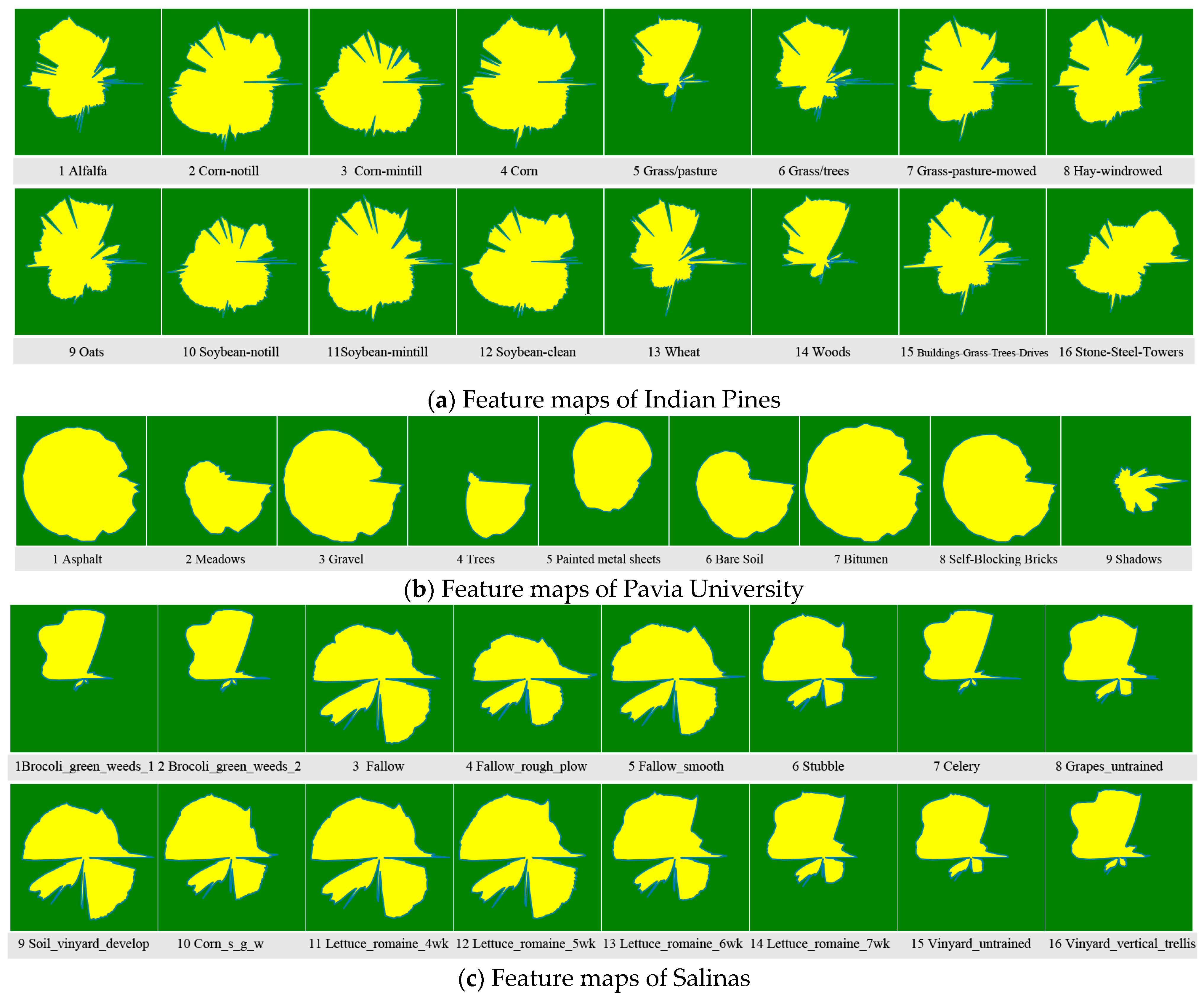
The eigenvalues of each band of the hyperspectral image are transformed into polarization feature maps utilizing the polar co-ordinate conversion method. This process converts each pixel’s spectral value into a polygon, capturing all original pixel information. These transformed feature maps then serve as a novel input form, facilitating direct training and classification within a classic 2D-CNN deep learning network model, such as VGG or ResNet;

(2)

Based on the feature maps generated in the previous step, a novel deep learning residual network model called DCFF-Net is introduced for training and classifying the converted spectral feature maps. This study includes comprehensive testing and validation across three hyperspectral datasets: Indian Pines, Pavia University, and Salinas. The proposed model consistently exhibits superior classification performance across these datasets through comparative analysis with other advanced pixel-based classification methods;

(3)

The response mechanism of DCFF-Net’s classification accuracy to polar co-ordinate maps under different filling methods is analyzed. The DCFF-Net model, evaluated using the pixel-patch input mode, is compared to other advanced models for classification performance, consistently demonstrating outstanding results.

2. Method

The classification methodology introduced in this study presents a novel approach by modifying the model’s data-input process, transforming pixel spectrum information within the hyperspectral image into graphical representations, and utilizing these as input data for model training and classification. The entire model primarily consists of two core components. The first component standardizes the pixel spectroscopy information into graphical data, with detailed processing methods outlined in Section 2.1. The second component involves training and classifying the transformed graphical data using the newly developed classification model, with comprehensive details regarding the model’s framework structure provided in Section 2.2.

2.1. Converting Hyperspectral Pixels into Feature Maps

Traditional hyperspectral data classification relies on vector space and is described as the data matrix. Each sample is considered a vector or point within a defined Euclidean space, ignoring the spatial relationships among the spectral values of each band in the pixel. The spectrum feature map of the image records not only the spectral values of the bands in the pixel but also the spatial relationships between these spectral values. This study introduces a new method for converting to a feature map, transforming the spectral classification problem into one of image recognition. Initially, the polar value normalization method is employed to standardize all bands of hyperspectral images, as calculated in Equation (1). Then, all the standardized optical spectral values of each pixel are converted into a polar co-ordinate diagram to form a two-dimensional polygon (Figure 1).

$${p\prime }_{i,j,k}={\displaystyle \frac{p_{i,j,k}-{\sigma }_k}{max\left\{p_{i,j,1}{,p}_{i,j,2},\cdots ,p_{i,j,k}\right\}-min\left\{p_{i,j,1}{,p}_{i,j,2},\cdots ,p_{i,j,k}\right\}}}$$

(1)

where $p_{i,j,k}$ is the spectral value of the k-th band of pixels in the i-th row and j-th column before normalization; ${p\prime }_{i,j,k}$ is the spectral values after the normalization; ${\sigma }_k$ is the average value of the k-th band.

The co-ordinate origin (0, 0) was employed to calculate the polar co-ordinate values of the spectral values for each band. In addition, the polar co-ordinate rotation angle, ${\theta }_k$, is determined based on the number of bands in the hyperspectral data, and $n$ represents the number of bands. The calculation method proceeds as follows:

$${\theta }_k={\displaystyle \frac{2\pi }{n}}\times k(k=\mathrm{0,1}, ,n-1)$$

(2)

The following formula calculates the co-ordinates $\left(x_k,y_k\right)$:

$$\begin{gathered} x_k=\cos {\theta }_k\times {p\prime }_{i,j,k} \\ {y}_k=\sin {\theta }_k\times {p\prime }_{i,j,k} \end{gathered}$$

(3)

The co-ordinate starting point of the feature maps in this study originates from the positive direction of the x–axis and involves counter-clockwise rotation, and neighboring co-ordinate points are connected with straight lines. Ultimately, the first and last co-ordinates are connected to form a closed polar co-ordinate graph. After extensive experimentation, the output graph size is set at 224 × 224 × 3.

In the process of converting spectral data into feature maps, hyperspectral imaging (HSI) data and corresponding label data are read simultaneously. The converted feature maps are standardized and annotated to include label information and pixel IDs. IDs are assigned sequentially starting from the top-left corner of the image matrix, proceeding row-wise from top to bottom and column-wise from left to right, with IDs ranging from 0 to H × W − 1. Here, H and W denote the height and width of the image data, respectively. According to the label category of each feature map, the feature maps of the same category were saved into corresponding folders. For instance, the Indian Pines dataset, which includes 16 categories, results in 16 folders containing labeled feature maps. Categories are labeled consistently with those in the image, ranging from 1 to 16, while unlabeled data are categorized as 0 and stored separately. During image prediction, there is an option to predict unlabeled data, which can significantly reduce prediction time. Alternatively, predictions can be made for all feature maps, albeit at the cost of increased processing time. Following prediction, the results are mapped back to an image format based on the ID information within the feature maps.

The method described above transforms pixels from hyperspectral images into feature maps. Figure 1 displays typical feature figures from the three datasets. Variations in sensors and bands among these hyperspectral datasets result in differing characteristics of the hyperspectral feature maps. The method only shows typical feature maps for each land type. In practice, features of the same terrain type vary, exhibiting distinct differences. Within a specific dataset, hyperspectral feature maps of different land types share similarities in their overall characteristics while exhibiting unique local details. These similarities provide an effective basis for classifying various hyperspectral feature maps. Similar spectral feature patterns are observed across different locations, especially in the Indian Pines dataset. Among the 16 types of characteristic graphic, such as 5-Grass/Pasture, Figure 1 highlights shape features where approximately one-third of the patterns resemble 7-Grass-Pasture-Mowed. This similarity is also noted in the nine types of characteristic graphic computed from the Pavia University datasets, although with larger and more varied overall sizes and shapes. In the Salinas dataset, characteristic graphics predominantly take two forms: butterfly-like and jellyfish-like, with notable similarities observed in the sizes of 8-Grapes_untrained and 15-Vineyard_untrained.

2.2. Network Architectures

Deep Context Feature Fusion Network (DCFF-Net) is proposed for the classification of hyperspectral feature diagrams. This network consists of three essential modules: Special Information Embedding (SIE, Figure 2b), Deep Special Feature Extraction (DSFE, Figure 2c), and Context Information Fusion (CIF, Figure 2a). To streamline the model parameters, the input image undergoes a 7 × 7 convolution followed by batch normalization, ReLU activation, and max-pooling. The resulting computations are then fed into the SIE and DSFE modules. The DSFE module extracts high-level feature representations of the spectral feature diagrams through a sequence of convolutional and batch normalization operations, followed by max-pooling. Then, the CIF module integrates the features from the SIE and DSFE modules. The output from this fusion process undergoes further processing through the SIE module. After passing through four layers of DSFE and CIF modules, max-pooling and global average pooling are applied to enrich the characteristic features. Finally, following the fully connected layer, the classification outcome is obtained through the softmax activation function.

The CIF module serves to seamlessly amalgamate context information, effectively integrating characteristics from various levels and yielding the ultimate feature representation for different pixels. Within the spectral feature extraction module, the features extracted by DSFE are bifurcated, with a portion integrated into the SIE module for contextual feature integration, while the remainder proceeds to the subsequent DSFE module. Figure 1 provides a simplified representation of the network architecture. Following each convolutional operation in the model, batch normalization and ReLU activation are applied. CIF comprises five distinct SIE modules and four DSFE and SIE fusion layers.

2.2.1. Spectral Information Embedding

With the advent of residual networks, the potential for deep learning network layers has substantially increased, leading to enhanced network depth and improved classification outcomes [39]. The Spectral Information Embedding (SIE) is configured as a residual block that includes a Squeeze and Excitation (SE) self-attention mechanism [61]. These residual blocks accelerate network training and mitigate challenges such as vanishing and exploding gradients. In the SIE module, the input x first undergoes a 3 × 3 convolution, batch normalization, and ReLU activation. Then, the SE Attention operation integrates all channels to enhance those contributing significantly to the classification task. Further convolution and batch normalization are then performed. When the stride in the input parameter is 1, the results are added back to the input layer. If the stride is greater than 1, a 1 × 1 convolution is applied to restore the size of the convolutional layer before adding it to the input layer to achieve the final feature encoding, which is then activated using the ReLU function. The specific structure is illustrated in Figure 2b.

The residual block is the basic module in the residual network model structure. The function can be expressed as follows:

$$F\left(x\right)=H\left(x\right)+x$$

(4)

where $H\left(x\right)$ is the residual function, which can be regarded as the part that performs a non-linear transformation on the input $x$. The addition operation in the formula means adding the input $x$ and the output of the residual function $H\left(x\right)$ to $F\left(x\right)$, which obtains the output of the residual block.

Convolutional layer operations form the core of deep learning. To enhance model performance, researchers have proposed several processing methods, such as batch normalization (BN) [62], activation functions [63], maximum pooling, and average pooling. These methods improve the model’s overall performance in different ways. The BN and ReLU activation functions are widely used in deep learning models. Batch normalization reduces the distribution variance across different data batches, mitigates gradient vanishing or explosion issues, and improves the training effect, generalization capability, and robustness of the deep neural network model. The ReLU activation function, known for its simplicity, speed, and effectiveness, significantly enhances model accuracy and convergence speed, demonstrating strong performance in numerous deep learning models.

The formulas for these functions are defined as follows:

$$X_n={\displaystyle \frac{x-\overline{x}}{\sqrt{s+\epsilon }}}$$

(5)

where $\overline{x}$ is mean; $s$ is the total variance; $\epsilon$ is a small positive number to avoid division by zero. The Relu activation function is defined as follows:

$$f\left(x\right)=max\left(0,x\right)$$

(6)

where $x$ is the element value in the input tensor. For input values greater than or equal to 0, the original value is output; for input values less than 0, the output value is 0.

2.2.2. Deep Spectral Feature Extract

After each convolutional computation, batch normalization and ReLU activation are applied, and a maximum pooling operation is employed to extract image features. This module employs a two-layer 3 × 3 convolutional calculation, incorporating the SE-Attention module to reconstruct the characteristics of different channels. It connects the feature map after the initial convolutional layer with that of the SE-Attention and subsequently with the feature map after the final convolutional layer to produce the ultimate feature map output of the DSFE module.

The max pooling layer preserves the most significant features and reduces the spatial dimension, diminishing the model’s sensitivity to spatial location, decreasing the number of parameters, and improving computational efficiency. Max pooling methods reduce the feature map size through down-sampling operations, allowing the model to learn overall features and local invariance, enhancing the model’s robustness and generalization capability. For example, if the input two-dimensional feature map size is (H, W), the pooling operation employs a window of size $\mathrm{k}$ × $\mathrm{k}$ and a step size of $\mathrm{s}$. Hence, the size of the feature map output by the pooling is ($⌊{\displaystyle \frac{H-k}{s}}⌋+1$, $⌊{\displaystyle \frac{W-k}{s}}⌋+1$), and the maximum pooling formula is defined as follows:

$$Y_{i,j}=\underset{p=0}{\overset{k-1}{\max }}\underset{q=0}{\overset{k-1}{\max }}{X}_{i\times s+p,j\times s+q},i=0,\dots ,⌊{\displaystyle \frac{H-k}{s}}⌋,j=0,\dots ,⌊{\displaystyle \frac{W-k}{s}}⌋$$

(7)

where $i$ and $j$ are the row and column index of the output feature map, respectively, and $p$ and $q$ are the row and column index in the pooling window, respectively. The function represents taking the maximum value in the window.

2.2.3. Cross-Entropy Loss Function and Activation Function

Cross-Entropy Loss is a commonly used metric in classification tasks to evaluate the difference between predicted outcomes and actual labels. It draws on the concept of cross-entropy in information theory, assessing the performance of a model by calculating the difference between the predicted probability distribution and the true label distribution. During the training process, model parameters are refined by minimizing the cross-entropy loss function, enabling more accurate predictions of the real labels. Optimization algorithms such as Gradient Descent are frequently employed to update model parameters based on the gradient of the loss function, thereby reducing the loss function. The mathematical expression for sparse categorical cross-entropy loss function is presented in Equation (8):

$$L\left(y,\widehat{y}\right)=-\sum _{i=1}^k{y}_i\log \left(\widehat{y_i}\right)$$

(8)

where $y$ is the probability distribution of the real label; $\widehat{y}$ is the predicted probability distribution of the model; $k$ is the number of categories.

The softmax activation function was employed following the fully connected layer in DCFF-NET. This function is typically utilized in the output layer of multi-classification challenges, converting the model’s initial outputs into a probability distribution. Each category’s probability value range is between 0 and 1, with the total probability across all categories summing to 1. The formula for the softmax function is provided below:

$$\sigma \left(xi\right)={\displaystyle \frac{e^{xi}}{{\sum }_{j=1}^k{e}^{xj}}},i=\mathrm{1,2},\cdots ,k$$

(9)

where $xi$ is the value of the i-th element in the input vector; $k$ is the number of categories; $\mathsf{\sigma }\left(xi\right)$ is the predicted probability of the i-th category.

The output from the softmax activation function delivers a probability value for each category, with the category exhibiting the highest probability designated as the final recognized category. The formula for this determination is specified below:

$$Class\left(X\prime \right)=arg max P_i,i=\mathrm{1,2},\cdots ,k$$

(10)

3. Results and Analysis

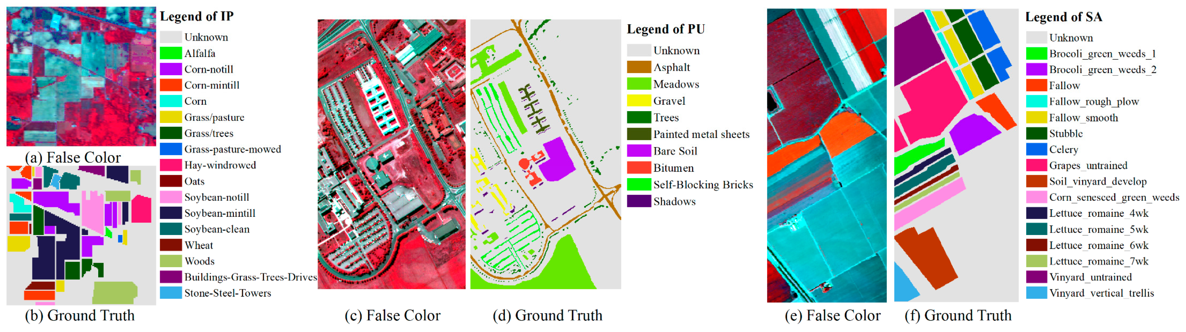
3.1. Experimental Datasets and Implementation

The Indian Pines (IP) Aerial hyperspectral dataset, collected by the AVIRIS sensor on 12 June 1992, encompasses an area of 2.9 km × 2.9 km in northwest Indiana. The dataset features a pixel size of 145 × 145 (21,025 pixels), a spatial resolution of 20 m, a spectral range from 0.4 to 2.5 µm, and includes 16 land cover types, predominantly in agricultural regions. Originally comprising 220 bands, the dataset was refined to 200 bands after excluding 20 bands that captured atmospheric water absorption and exhibited low SNR. The retained data from these 200 bands were utilized in this experiment.

Table 1. Detailed information of three datasets.

Classes	Indian Pines		Salinas		Pavia University
	Names	Samples	Names	Samples	Names	Samples
1	Alfalfa	46	Brocoli_green_weeds_1	2009	Asphalt	6631
2	Corn-no till	1428	Brocoli_green_weeds_2	3726	Meadows	18,649
3	Corn-min till	830	Fallow	1976	Gravel	2099
4	Corn	237	Fallow_rough_plow	1394	Trees	3064
5	Grass-pasture	483	Fallow_smooth	2678	Painted metal sheets	1345
6	Grass-trees	730	Stubble	3959	Bare Soil	5029
7	Grass-pasture-mowed	28	Celery	3579	Bitumen	1330
8	Hay-windrowed	478	Grapes_untrained	11,271	Self-Blocking Bricks	3682
9	Oats	20	Soil_vinyard_develop	6203	Shadows	947
10	Soybean-no till	972	Corn_senesced_green_weeds	3278	-	-
11	Soybean-min till	2455	Lettuce_romaine_4wk	1068	-	-
12	Soybean-clean	593	Lettuce_romaine_5wk	1927	-	-
13	Wheat	205	Lettuce_romaine_6wk	916	-	-
14	Woods	1265	Lettuce_romaine_7wk	1070	-	-
15	Buildings-Grass-Trees-Drives	386	Vinyard_untrained	7268	-	-
16	Stone-Steel-Towers	93	Vinyard_vertical_trellis	1807	-	-
	Total Samples	10,249		54,129		42,956

and Figure 3a,b illustrate the actual marking information of ground objects in this dataset. The sample distribution across different types is highly variable, with quantities ranging from 20 to 2455.

Aerial hyperspectral remote sensing images of Pavia University (PU) were obtained by the German airborne Reflective Optical Spectral Imager (ROSIS) on 8 July 2002 in the campus area of the University of Pavia, Italy. The spatial resolution of the data is 1.3 m, the image size is 610 × 340 pixels (207,400 pixels), and the spectral range of the image spans from 0.43 to 0.86 µm, encompassing 115 spectral channels. The dataset includes nine urban land cover types and 42,776 labeled pixels. The image on the right displays a false-color composite image of the Pavia University data and the actual overlay type of the surface. Due to noise, 12 noise bands were eliminated, leaving 103 bands to verify the performance of the proposed method. The PU dataset contains nine categories of ground objects, as shown in Figure 3c,d.

The Salinas dataset (SA) consists of hyperspectral remote sensing images of the Salinas Valley region in southern California, United States, acquired by the AVIRIS sensor. The image measures 512 × 217 pixels, with a spatial resolution of 3.7 m, a spectral resolution of between 9.7 and 12 nm, and a spectral range from 400 to 2500 nm. It includes 16 types of ground objects and 54,129 labeled samples. The dataset initially had 224 bands, but 20 bands affected by atmospheric water absorption and low signal-to-noise ratios were removed. The remaining 204 bands, retained after processing, were utilized in this experiment, as indicated in Figure 3e,f.

All experiments were conducted in identical environments using two computers. The configuration for these computers was as follows: the hardware platform included an Intel Core i7-9700K (8 cores/8 threading)/i7-1100F (8 cores/16 threading) processor with 12M/16M L3-cache/, 64 GB/128 G DDR4 memory at 3200 MHz serial speed, NVIDIA GeForce RTX 2070 GPU with 8 GB DDR5/RTX 3060 GPU with 12 GB DDR5 video memory, and a 1 TB HDD with 7200 RPM. The software platform comprised the Windows 10 Professional operating system, Keras 2.5.0 based on TensorFlow-gpu 2.5.0, and Python 3.7.7. The SF-Pixel model used the parameters specified in [51], while other models were trained using a batch size of 12, with IP models employing an Adam optimizer with a learning rate of 2 × 10⁻³, a decay of 1 × 10⁻⁴, and PU and SA models using a learning rate of 1 × 10⁻⁴ and a decay of 1 × 10⁻⁵.

3.2. Evaluation Criterion

Classification accuracy was estimated using evaluation indicators such as overall accuracy (OA), average accuracy (AA) for each category, user accuracy (UA) for each category, and kappa coefficient (KA) [64,65]. In this text, percentages represent the KA. The calculation formula is as follows:

$$OA=\sum _{j-1}^N{\displaystyle \frac{{TP}_j+{TN}_j}{{TP}_j+{TN}_j+{FP}_j+{FN}_j}}$$

(11)

$$AA={\displaystyle \frac{1}{N}}\sum _{j-1}^N{\displaystyle \frac{{TP}_j}{{TP}_j+{FN}_j}}$$

(12)

$${UA}_j={\displaystyle \frac{{TP}_j}{{TP}_j+{FN}_j}}$$

(13)

$$KA={\displaystyle \frac{p_0{-p}_e}{1{-p}_e}}$$

(14)

where $j$ is the class $j$; ${TP}_j$ (True Positive) is the number of true examples, i.e., the number of samples that are correctly classified as positive examples; ${TN}_j$ (True Negative) is the number of true counterexamples, i.e., the number of samples that are correctly classified as negative examples; ${FP}_j$ (False Positive) is the number of false positives. The number of examples is the number of samples that were incorrectly classified as positive examples; ${FN}_j$ (False Negative) is the number of false counterexamples, that is, the number of samples that were incorrectly classified as negative examples; $\mathrm{N}$ is the total number of categories; $p_0$ is the accuracy of the classifier; $p_e$ is the random accuracy that the classifier can achieve.

3.3. Results Analysis Based on Feature Map

Traditional Naive Bayes (NB), K-Nearest Neighbors (KNN), Random Forest (RF), and Multi-Layer Perceptron (MLP), 1D-CNN, VGG16, ResNet50, and SF based on pixel-wise (SF-Pixel) deep learning methods were selected for comparative analysis with DCFF-NET. NB, KNN, and RF are all open-source machine learning libraries in Python. The data partitioning for random seeds was set to fixed values to achieve data recovery. NB, KNN, and RF use automatic searches (Grid Search) to select the optimal parameters with a 50%-off verification method. MLP, 1D-CNN, VGG16, ResNet50, and DCFF-Net methods were implemented using TensorFlow2.5.0, and a grid search algorithm was also employed to obtain optimal parameters, such as batch size, learning rate, and decay. SF-Pixel utilized publicly available code and made modifications according to the experiments described. The VGG16 and ResNet50 models and pre-trained weights were not used. Instead, training and prediction were conducted using feature maps. When using a grid search method, important parameter selection was performed first, reducing the parameter-space range and gradually narrowing the search range of the parameters based on the calculation results to improve search efficiency. This study uses different proportions of training samples for training and prediction. As the proportion of the training sample changed, the training process and performance of the model were also affected. Therefore, under different training sample proportions, the best parameter combination is sought to ensure the best performance and generalization ability of the model. The best parameters and optimal models were selected to predict and evaluate the three hyperspectral datasets.

The results are depicted in

Table 2. Accuracies (%) of each method with different training samples on three datasets.

Methods	Train /Test	IP			PU			SA
		OA	KA	AA	OA	KA	AA	OA	KA	AA
NB	30%/70%	71.58	66.96	53.85	90.91	87.79	87.39	91.13	90.10	94.22
KNN		79.98	77.12	79.09	90.28	86.94	88.29	92.24	91.36	96.10
RF		83.17	80.66	73.67	91.91	89.17	89.39	93.39	92.63	96.39
MLP		77.65	74.52	77.12	93.88	91.86	90.31	92.31	91.43	95.67
1DCNN		79.90	76.94	76.65	93.97	92.00	92.42	93.34	92.58	96.91
SF-Pixel		85.49	83.39	82.80	93.95	92.02	92.56	92.71	91.87	96.33
VGG16		85.18	83.16	83.21	92.19	89.64	89.56	94.25	93.59	96.66
Resnet50		82.13	79.60	77.71	93.44	91.28	90.49	94.62	94.01	97.23
DCFF-NET		86.68	85.04	85.08	94.73	92.99	92.60	95.14	94.59	97.48
NB	20%/80%	66.14	60.52	48.63	89.36	85.61	85.24	90.21	89.09	93.37
KNN		78.12	75.00	76.38	89.34	85.61	87.25	91.38	90.40	95.54
RF		80.75	77.85	66.60	91.04	87.95	88.05	92.60	91.75	95.90
MLP		75.20	71.53	71.95	92.37	89.95	90.56	91.34	90.34	94.60
1DCNN		73.88	69.59	68.63	93.07	90.82	89.79	92.33	91.43	96.29
SF-Pixel		82.91	80.38	76.87	92.77	90.50	91.41	91.62	90.68	95.80
VGG16		83.44	81.12	83.25	92.83	90.48	89.64	92.55	91.68	95.73
Resnet50		75.84	72.44	73.64	93.23	91.00	90.89	93.80	93.10	96.48
DCFF-NET		84.05	81.77	79.90	94.11	92.18	91.86	94.24	93.58	96.81
NB	10%/90%	58.05	50.08	40.93	85.85	80.67	79.52	88.22	86.86	91.49
KNN		74.76	71.20	70.97	87.53	83.12	85.01	90.03	88.90	94.42
RF		75.87	72.27	60.42	89.52	85.86	85.79	91.31	90.31	94.93
MLP		69.20	64.93	60.60	92.02	89.40	89.34	90.41	89.35	94.91
1DCNN		69.36	64.98	64.48	92.71	90.39	90.85	91.55	90.58	94.98
SF-Pixel		75.27	71.47	64.44	90.71	87.72	89.58	90.00	88.87	94.89
VGG16		77.88	74.73	72.80	91.59	88.84	88.61	92.12	91.23	95.50
Resnet50		70.90	66.54	64.14	91.51	88.73	89.18	92.35	91.47	94.86
DCFF-NET		78.21	75.07	84.36	92.56	90.40	90.39	93.00	92.20	95.66

. When various classification methods use different training sample ratios, the accuracy of image prediction results increases significantly as the proportion of training samples increases. The DCFF-Net classification method performs well on the three datasets. The three different datasets exhibit higher performance than the lower training ratios in the case of 10%, 20%, and 30% training ratios. Except for the maximum value of AA, all other values achieve the maximum value and demonstrate the best classification performance overall. With 30% training samples, the OA, KA, and AA of the IP datasets are 86.68%, 85.05%, and 85.08%; the OA, KA, and AA of the PU dataset are 94.73%, 92.99%, and 92.60%; and the OA, KA, and AA of the SA dataset are 95.14%, 94.59%, and 97.48%.

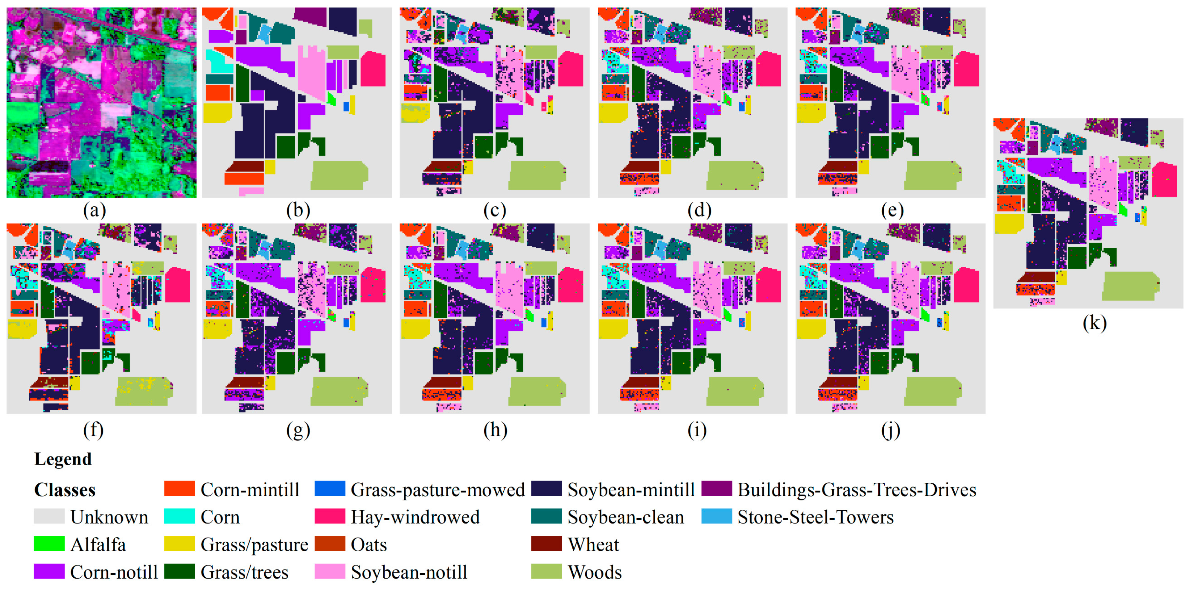
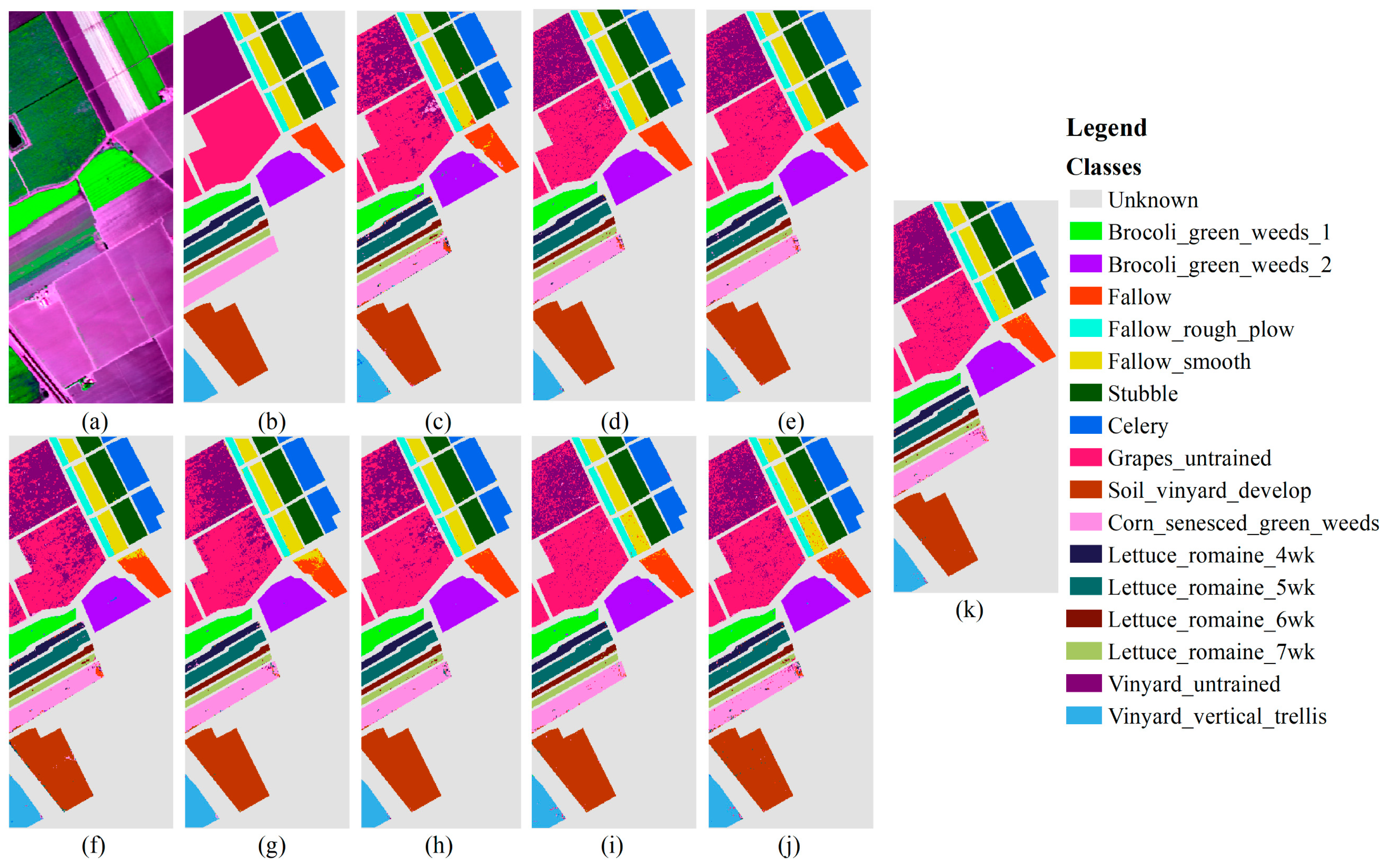
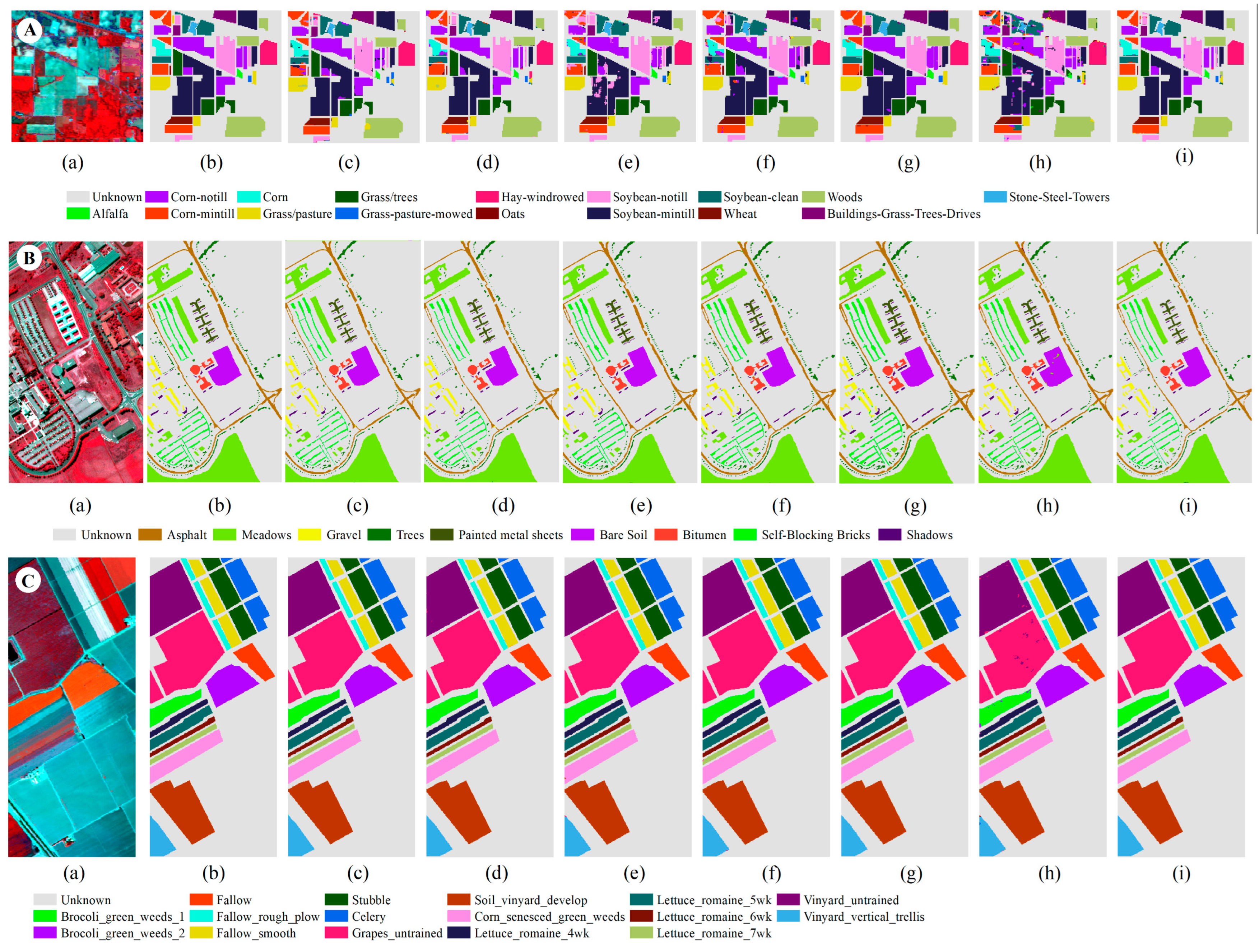
3.3.1. Results of Indian Pines

Figure 4 and

Table 3. Accuracies (%) of labeled samples per class for the Indian Pines dataset (30% Train Samples).

Classes Name	Train/Test	NB	KNN	RF	MLP	1DCNN	SF-Pixel	VGG16	Resnet50	DCFF-NET
Alfalfa	13/33	0.00	69.70	66.67	82.61	15.62	78.79	90.32	92.00	92.00
Corn-no till	428/1000	60.60	70.00	76.90	47.62	73.30	80.20	77.27	71.49	83.48
Corn-min till	249/581	39.07	65.58	60.24	70.24	72.98	78.01	86.70	82.30	84.42
Corn	71/166	13.25	59.04	56.02	70.04	64.46	63.25	80.29	73.03	86.40
Grass-pasture	144/339	70.80	93.51	89.09	83.64	84.62	92.55	96.99	92.57	98.65
Grass-trees	219/511	97.06	96.09	96.67	89.86	95.50	96.88	93.43	95.59	95.71
Grass-pasture-mowed	8/20	0.00	85.00	40.00	85.71	95.00	87.50	76.49	66.67	72.03
Hay-windrowed	143/335	99.40	98.51	98.81	96.44	94.03	97.57	92.31	91.43	92.86
Oats	6/14	0.00	71.43	21.43	25.00	78.57	58.33	80.91	80.30	83.78
Soybean-no till	291/681	66.81	79.15	82.09	73.97	60.15	81.65	72.41	67.08	77.41
Soybean-min till	736/1719	87.32	82.32	90.87	82.00	84.47	87.62	66.46	61.63	75.00
Soybean-clean	177/416	38.22	62.50	69.71	77.07	72.53	76.34	92.26	92.66	92.66
Wheat	61/144	93.75	100.00	95.83	99.51	98.60	98.55	97.60	94.48	96.84
Woods	379/886	97.97	91.99	95.03	97.08	94.13	96.94	72.22	63.64	81.82
Buildings-Grass-Trees-Drives	115/271	16.97	54.24	57.56	60.62	56.30	55.27	98.58	99.70	100.00
Stone-Steel-Towers	27/66	80.30	86.36	81.82	92.47	86.15	95.38	57.14	18.75	56.25
OA	3067/7182	71.58	79.98	83.17	77.65	79.90	85.39	85.18	82.13	86.68
KA		66.96	77.12	80.66	74.52	76.94	83.39	83.16	79.60	85.04
AA		53.85	79.09	73.67	77.12	76.65	82.80	83.21	77.71	85.08

show the classification result chart obtained using 30% of the training samples from the Indian Pines dataset. The UAs of each category in this dataset are listed in Table 3. It can be observed from the table that, out of the 16 land types, seven types achieved the best classification effects compared to other classification methods when using the DCFF-Net classification method. The OA, KA, and AA were 86.68%, 85.04%, and 85.08%, respectively, higher than other classification methods. The classification effect of SF-Pixel and VGG16 was less than that of DCFF-Net, with OA, KA, and AA at 85.39%, 83.39%, 82.80, 85.18%, 83.16%, and 83.21%, respectively. Secondly, ResNet50 also performed well. These four deep learning methods outperformed other classification methods. The optimal UA values for the 16 land types were scattered across various classification methods and were not concentrated in a specific classification method. In some categories, such as Corn-no Till, Corn, Oats, and others, DCFF-Net achieved a better classification effect. The NB classification methods showed significant variation in UA across different categories. For Alfalfa, Grass-Pasture-Mowed, and Oats the UA was 0.00% due to too few samples, while the highest, Hay-Windrowed, reached an AA of 99.40%. However, the average accuracy across the 16 categories was only 53.85%, far lower than several other methods.

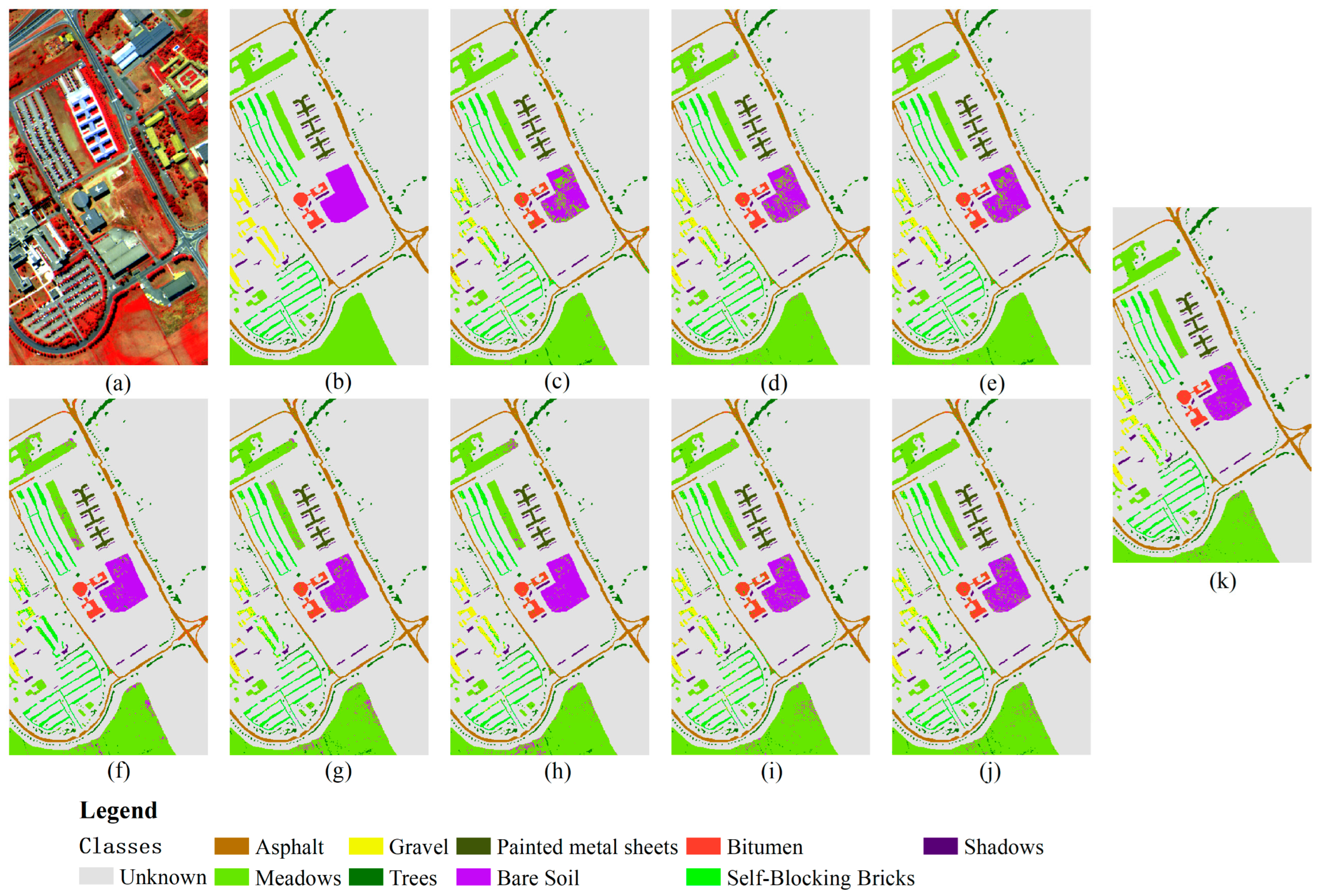
3.3.2. Results of Pavia University

Figure 5 illustrates the classification result diagram obtained using 30% training samples on the Pavia University dataset. The OA, KA, and AA of the DCFF-Net model were 94.73%, 92.99%, and 92.60%, respectively, and these three indicators achieved the highest classification accuracy, as shown in

Table 4. Accuracies (%) of labeled samples per class for the Pavia University dataset (30% train samples).

Class Name	Train/Test	NB	KNN	RF	MLP	1DCNN	SF-Pixel	VGG16	Resnet50	DCFF-NET
Asphalt	1989/4642	90.69	89.19	92.20	92.45	94.64	96.41	93.08	94.46	93.84
Meadows	5594/13,055	98.47	97.88	97.94	97.82	97.65	95.02	96.51	97.36	97.54
Gravel	629/1470	66.87	74.56	74.15	65.66	88.16	88.21	71.34	73.13	77.70
Trees	919/2145	90.26	88.21	91.93	95.22	94.03	95.14	91.01	95.44	96.00
Painted metal sheets	403/942	99.15	99.47	99.15	99.26	100.00	99.57	99.37	99.38	99.17
Bare Soil	1508/3521	74.07	69.33	77.08	90.62	92.53	96.13	89.75	90.58	92.02
Bitumen	399/931	77.23	87.76	81.95	75.68	86.47	77.88	80.53	77.63	88.05
Self-Blocking Bricks	1104/2578	89.91	88.17	90.11	93.15	78.27	85.47	84.75	87.01	88.35
Shadows	284/663	99.85	100.00	100.00	99.25	100.00	100.00	99.70	99.39	99.70
OA	12,829/29,947	90.91	90.28	91.91	92.70	93.97	93.95	92.19	93.44	94.73
KA		87.79	86.94	89.17	90.22	92.00	92.02	89.64	91.28	92.99
AA		87.39	88.29	89.39	89.90	92.42	92.56	89.56	90.49	92.60

. Trees and Bitumen’s UA were the highest compared to other methods. The 1D-CNN classification result’s OA was second only to DCFF-Net, reaching 93.97%. The categories Gravel, Painted Metal Sheets, Bare Soil, and Shadows were higher than other methods. For Gravel and Bitumen, no classification methods exceeded 90.00%. In Figure 1, Gravel, Bitumen, and Self-Blocking Bricks had similar ground features, leading to generally low UA in these categories. Among all comparison methods, the KNN classification method had the lowest accuracy.

3.3.3. Results of Salinas

Figure 6 presents the classification results obtained using 30% training samples on the Salinas dataset. The number of training samples is 16,231.

Table 5. Accuracies (%) of labeled samples per class for the Salinas dataset (30% train samples).

Classes Name	Train/Test	NB	KNN	RF	MLP	1DCNN	SF-Pixel	VGG16	Resnet50	DCFF-NET
Brocoli_green_weeds_1	602/1407	97.51	99.29	99.93	99.36	100.00	99.58	99.86	99.79	99.59
Brocoli_green_weeds_2	1117/2609	99.16	99.92	99.96	99.43	99.96	99.96	96.18	95.25	96.82
Fallow	592/1384	96.46	99.93	99.42	91.04	99.42	99.36	98.43	99.08	98.69
Fallow_rough_plow	418/976	99.08	99.39	99.39	99.08	99.18	99.47	98.12	99.41	99.48
Fallow_smooth	803/1875	96.48	98.51	98.77	98.72	99.20	99.37	94.71	99.06	99.22
Stubble	1187/2772	99.42	99.64	99.75	99.89	99.96	99.67	98.67	98.96	98.45
Celery	1073/2506	99.20	99.60	99.68	99.80	99.88	99.76	80.96	81.36	80.64
Grapes_untrained	3381/7890	87.93	85.02	89.91	79.62	86.43	90.43	97.17	98.65	98.96
Soil_vinyard_develop	1860/4343	99.06	99.52	99.36	98.83	99.93	99.91	98.66	99.77	99.92
Corn_senesced_green_weeds	983/2295	91.42	94.12	94.51	92.81	98.30	95.77	97.33	97.59	98.76
Lettuce_romaine_4wk	320/748	89.44	97.86	95.99	98.40	98.93	100.00	99.39	99.28	99.17
Lettuce_romaine_5wk	578/1349	99.56	99.85	99.41	85.17	99.48	100.00	98.97	99.05	99.31
Lettuce_romaine_6wk	274/642	97.82	98.75	98.44	97.66	99.38	99.84	99.78	99.74	99.93
Lettuce_romaine_7wk	321/749	92.79	96.66	97.06	97.46	97.33	94.71	99.88	99.68	99.52
Vinyard_untrained	2180/5088	65.33	71.29	72.27	78.83	73.92	64.34	88.61	89.51	91.71
Vinyard_vertical_trellis	542/1265	96.92	98.26	98.42	98.10	99.21	99.04	99.82	99.45	99.58
OA	16,231/37,898	91.13	92.24	93.39	91.13	93.34	92.71	94.25	94.62	95.14
KA		90.10	91.36	92.63	90.14	92.58	91.87	93.59	94.01	94.59
AA		94.22	96.10	96.39	94.64	96.91	96.33	96.66	97.23	97.48

shows the user accuracy (UA) of various types in SA. DCFF-Net classification OA, KA, and AA were 95.14%, 94.59%, and 97.48%, respectively, better than other comparison methods. VGG16 and ResNet50 also achieved better classification effects, second only to DCFF-Net. Among the 16 types of land, the DCFF-Net classification results were the highest in the UA of six places. Except for the low UA in Celery, the classification accuracy in other categories was not significantly different from other classification methods. The Celery UA was extremely low. Figure 6 indicates that the characteristic graphic features of Celery and Broccoli_green_weeds_1 and Broccoli_green_weeds_2 were highly similar, making them difficult to distinguish effectively and significantly low accuracy. In the current classification methods, Grapes_untrained and Vineyard_untrained are difficult to distinguish. As shown in Table 5, the three methods—DCFF-Net, VGG16, and ResNet50—were significantly higher than other classification methods. DCFF-Net significantly increased the characteristics of similar objects, obtaining higher classification accuracy. Grapes_untrained and Vineyard_untrained achieved 98.96% and 91.71%, respectively. In other methods, the UAs of Grapes_untrained and Vineyard_untrained were lower than 90.00%, with NB, KNN, RF, MLP, 1D-CNN, and other methods achieving less than 80.00%.

The eight classification methods mentioned in the text are NB, KNN, RF, MLP, 1D-CNN, SF-Pixel, VGG16, ResNet50, and DCFF-Net. The first six methods used one-dimensional serial vector data as the model input data, while the latter three were based on two-dimensional images. The latter three methods extracted image features through 2D-CNN, classifying the data into different categories. In the IP data concentration, including Corn-Min Till, Corn, Oats, and Buildings-Grass-Trees-Drives, and on the SA dataset, including Grapes_untrained and Vineyard_untrained, the accuracy of the latter three methods was significantly higher than the first five methods. This indicates that 2D-CNN can achieve better classification effects in some easily mixed categories. However, for some categories, the first five methods performed better than the latter three methods, such as Soybean-Min Till, Woods, and Stone-Steel-Towers in the IP dataset. More suitable classification methods can be selected based on these observations in practical applications.

3.4. Results Analysis Based on Pixel-Patched

An additional evaluation was conducted using the pixel-patched method to examine the classification effectiveness of DCFF-NET and assess the performance of the proposed model. The methods NB, KNN, RF, MLP, 1D-CNN, and SF-Pixel use one-dimensional vector data and cannot directly use pixels as input data. Therefore, a comparative analysis was conducted using HybridSN, 3D-CNN, A2S2KNet, and SF based on patch-wise (SF-Patch) models. The pixel patch size was uniformly extracted at 24 × 24 × C as the input data, where C is the number of image channels, and 10% of the categories were selected as training samples. The models underwent a fine-tuning process to facilitate the utilization of VGG16 and ResNet50 models for training and testing with the provided input data. After model training was completed, the optimal model was selected for testing, using 90% of the data as test data, performing the test 10 times. The average value and standard deviation were selected as the test results, as shown in

Table 6. Accuracies (%) of Indian Pines dataset.

Classes Name	Train/Test	VGG16	Resnet50	3-DCNN	HybridSN	A2S2K	SF-Patch	DCFF-NET
Alfalfa	4/42	100.00 ± 0.00	100.00 ± 0.00	100.00 ± 0.00	100.00 ± 0.00	93.50 ± 7.04	74.36 + 16.04	98.60 ± 1.15
Corn-no till	142/1286	96.68 ± 0.19	97.72 ± 0.10	90.86 ± 0.20	94.51 ± 0.20	97.45 ± 2.69	82.22 + 3.41	98.03 ± 0.14
Corn-min till	83/747	89.95 ± 0.26	96.48 ± 0.20	78.99 ± 0.29	93.47 ± 0.29	97.54 ± 1.63	87.75 + 4.63	99.62 ± 0.08
Corn	23/214	89.69 ± 0.63	84.84 ± 0.61	89.65 ± 1.16	69.14 ± 1.16	98.09 ± 1.30	89.95 + 9.67	95.54 ± 0.48
Grass-pasture	48/435	83.01 ± 0.84	89.3 ± 0.39	92.94 ± 0.24	94.3 ± 0.24	99.66 ± 0.31	88.01 + 2.47	87.01 ± 0.40
Grass-trees	73/657	99.08 ± 0.10	97.56 ± 0.18	100.00 ± 0.00	99.02 ± 0.10	99.28 ± 0.91	96.73 + 3.27	100.00 ± 0.00
Grass-pasture-mowed	2/26	100.00 ± 0.00	100.00 ± 0.00	88.54 ± 0.00	100.00 ± 0.00	90.63 ± 13.26	68.00 + 33.5	100.00 ± 0.00
Hay-windrowed	47/431	100.00 ± 0.00	100.00 ± 0.00	100.00 ± 0.00	100.00 ± 0.00	99.57 ± 0.60	94.68 + 2.29	99.77 ± 0.00
Oats	2/18	100.00 ± 0.00	100.00 ± 0.00	95.54 ± 0.00	100.00 ± 0.00	72.22 ± 20.79	66.67 + 27.4	100.00 ± 0.00
Soybean-no till	97/875	95.85 ± 0.08	98.29 ± 0.12	100.00 ± 0.20	95.94 ± 0.20	97.59 ± 0.97	84.25 + 3.09	96.90 ± 0.14
Soybean-min till	245/2210	98.63 ± 0.08	99.57 ± 0.05	88.44 ± 0.08	96.5 ± 0.08	99.11 ± 0.51	92.72 + 1.66	99.25 ± 0.07
Soybean-clean	59/534	91.56 ± 0.32	95.24 ± 0.23	93.28 ± 0.40	89.1 ± 0.40	98.52 ± 1.32	71.40 + 3.85	95.47 ± 0.22
Wheat	20/185	99.61 ± 0.25	98.97 ± 0.17	100.00 ± 0.00	100.00 ± 0.00	97.47 ± 1.46	94.51 + 5.45	100.00 ± 0.00
Woods	126/1139	96.14 ± 0.20	99.82 ± 0.00	99.91 ± 0.12	98.9 ± 0.12	99.55 ± 0.51	96.74 + 1.24	99.84 ± 0.03
Buildings-Grass-Trees-Drives	38/348	99.45 ± 0.09	99.02 ± 0.18	100.00 ± 0.00	97.91 ± 0.17	95.04 ± 3.20	77.84 + 7.96	100.00 ± 0.00
Stone-Steel-Towers	9/84	91.22 ± 0.80	83.69 ± 1.15	94.16 ± 1.24	85.64 ± 1.24	94.36 ± 6.10	75.00 + 16.17	93.67 ± 0.80
OA	1018/9231	95.82 ± 0.075	97.6 ± 0.039	93.18 ± 0.069	95.46 ± 0.063	98.29 ± 0.345	88.50 + 0.802	98.15 ± 0.036
KA		95.24 ± 0.084	97.26 ± 0.045	92.26 ± 0.079	94.81 ± 0.072	98.05 ± 0.394	86.86 + 0.907	97.89 ± 0.041
AA		95.68 ± 0.094	96.28 ± 0.105	94.52 ± 0.168	94.65 ± 0.123	95.60 ± 0.649	83.80 + 3.993	97.73 ± 0.092

,

Table 7. Accuracies (%) of Pavia University dataset.

Classes Name	Train/Test	VGG16	Resnet50	3-DCNN	HybridSN	A2S2K	SF-Patch	DCFF-NET
Asphalt	663/5968	99.49 ± 0.03	99.45 ± 0.03	99.76 ± 0.01	99.24 ± 0.03	99.91 ± 0.08	98.67 ± 0.58	99.89 ± 0.01
Meadows	1864/16,785	99.97 ± 0.01	99.98 ± 0.00	99.95 ± 0.01	99.98 ± 0.00	99.97 ± 0.02	99.86 ± 0.08	99.92 ± 0.01
Gravel	209/1890	99.77 ± 0.03	99.66 ± 0.03	99.85 ± 0.02	97.49 ± 0.09	99.80 ± 0.28	95.84 ± 1.23	100.00 ± 0.00
Trees	306/2758	98.10 ± 0.06	98.43 ± 0.04	99.32 ± 0.05	99.62 ± 0.03	99.96 ± 0.06	97.21 ± 0.67	99.17 ± 0.04
Painted metal sheets	134/1211	99.93 ± 0.03	100.00 ± 0.00	100.00 ± 0.00	100.00 ± 0.00	99.97 ± 0.04	100.00 ± 0.00	100.00 ± 0.00
Bare Soil	502/4527	100.00 ± 0.00	100.00 ± 0.00	100.00 ± 0.00	99.83 ± 0.01	99.93 ± 0.06	99.74 ± 0.06	100.00 ± 0.00
Bitumen	133/1197	98.71 ± 0.11	98.63 ± 0.10	99.35 ± 0.10	96.98 ± 0.14	99.97 ± 0.04	95.41 ± 1.45	99.20 ± 0.06
Self-Blocking Bricks	368/3314	99.75 ± 0.02	99.96 ± 0.02	99.89 ± 0.01	99.76 ± 0.03	98.44 ± 1.13	97.34 ± 0.34	100.00 ± 0.00
Shadows	94/853	99.26 ± 0.08	99.14 ± 0.09	99.88 ± 0.00	99.89 ± 0.04	99.74 ± 0.21	98.59 ± 0.26	99.91 ± 0.05
OA	4273/38,503	99.68 ± 0.007	99.71 ± 0.007	99.85 ± 0.007	99.58 ± 0.004	99.81 ± 0.093	98.89 ± 0.164	99.86 ± 0.004
KA		99.58 ± 0.009	99.62 ± 0.009	99.80 ± 0.009	99.45 ± 0.005	99.75 ± 0.123	98.07 ± 0.235	99.82 ± 0.006
AA		99.44 ± 0.013	99.47 ± 0.016	99.78 ± 0.014	99.20 ± 0.017	99.74 ± 0.103	98.53 ± 0.213	99.79 ± 0.011

and

Table 8. Accuracies (%) of Salinas dataset.

Classes Name	Train/Test	VGG16	Resnet50	3-DCNN	HybridSN	A2S2K	SF-Patch	DCFF-NET
Brocoli_green_weeds_1	200/1809	100.00 ± 0.00	100.00 ± 0.00	100.00 ± 0.00	100.00 ± 0.00	100.00 ± 0.00	98.78 ± 0.84	100.00 ± 0.00
Brocoli_green_weeds_2	372/3354	100.00 ± 0.00	100.00 ± 0.00	100.00 ± 0.00	100.00 ± 0.00	100.00 ± 0.00	99.91 ± 0.04	100.00 ± 0.00
Fallow	197/1779	100.00 ± 0.00	99.89 ± 0.02	99.96 ± 0.02	100.00 ± 0.00	100.00 ± 0.00	99.72 ± 0.13	100.00 ± 0.00
Fallow_rough_plow	139/1255	99.86 ± 0.03	100.00 ± 0.00	100.00 ± 0.00	99.92 ± 0.00	99.82 ± 0.15	99.84 ± 0.09	99.94 ± 0.03
Fallow_smooth	267/2411	99.88 ± 0.01	99.70 ± 0.03	99.88 ± 0.02	99.81 ± 0.02	99.95 ± 0.04	100.00 ± 0.00	99.96 ± 0.01
Stubble	395/3564	99.96 ± 0.02	100.00 ± 0.00	100.00 ± 0.00	100.00 ± 0.00	100.00 ± 0.00	100.00 ± 0.00	100.00 ± 0.00
Celery	357/3222	100.00 ± 0.00	100.00 ± 0.00	100.00 ± 0.00	100.00 ± 0.00	100.00 ± 0.00	99.63 ± 0.26	99.97 ± 0.00
Grapes_untrained	1127/10,144	100.00 ± 0.00	100.00 ± 0.00	99.98 ± 0.01	99.96 ± 0.01	99.95 ± 0.03	99.17 ± 0.54	99.99 ± 0.00
Soil_vinyard_develop	620/5583	100.00 ± 0.00	100.00 ± 0.00	100.00 ± 0.00	100.00 ± 0.00	99.97 ± 0.03	99.80 ± 0.03	100.00 ± 0.00
Corn_senesced_green_weeds	327/2951	99.60 ± 0.03	100.00 ± 0.00	99.81 ± 0.02	99.83 ± 0.04	99.94 ± 0.09	99.93 ± 0.05	100.00 ± 0.00
Lettuce_romaine_4wk	106/962	100.00 ± 0.00	100.00 ± 0.00	99.51 ± 0.05	100.00 ± 0.00	100.00 ± 0.00	98.96 ± 0.75	99.24 ± 0.08
Lettuce_romaine_5wk	192/1735	100.00 ± 0.00	100.00 ± 0.00	99.91 ± 0.03	100.00 ± 0.00	100.00 ± 0.00	100.00 ± 0.00	100.00 ± 0.00
Lettuce_romaine_6wk	91/825	100.00 ± 0.00	99.88 ± 0.00	99.89 ± 0.04	99.90 ± 0.05	99.96 ± 0.06	99.88 ± 0.13	100.00 ± 0.00
Lettuce_romaine_7wk	107/963	100.00 ± 0.00	100.00 ± 0.00	100.00 ± 0.00	99.61 ± 0.04	99.61 ± 0.55	99.79 ± 0.21	100.00 ± 0.00
Vinyard_untrained	726/6542	99.99 ± 0.00	99.82 ± 0.02	100.00 ± 0.00	100.00 ± 0.00	99.85 ± 0.18	98.67 ± 0.73	100.00 ± 0.00
Vinyard_vertical_trellis	180/1627	99.82 ± 0.02	100.00 ± 0.00	99.71 ± 0.03	99.77 ± 0.03	100.00 ± 0.00	99.38 ± 0.63	100.00 ± 0.00
OA	5403/48,726	99.95 ± 0.003	99.96 ± 0.003	99.95 ± 0.002	99.95 ± 0.003	99.95 ± 0.032	99.48 ± 0.085	99.98 ± 0.002
KA		99.95 ± 0.003	99.95 ± 0.003	99.95 ± 0.002	99.95 ± 0.003	99.94 ± 0.036	99.43 ± 0.097	99.98 ± 0.003
AA		99.94 ± 0.003	99.96 ± 0.002	99.92 ± 0.004	99.92 ± 0.004	99.94 ± 0.039	99.59 ± 0.105	99.94 ± 0.006

. Figure 7 shows the classification map for each classification method. The OA and KA on the IP dataset were 98.15% and 97.89%, respectively, second only to A2S2K but higher than all other methods. The AA value of 97.73% was the highest of all methods. The OA, KA, and AA of 3D-CNN were the lowest, with values of 93.18%, 92.26%, and 94.52%, respectively. The DCFF-Net model achieved the best classification performance regarding OA, KA, and AA on the PU and SA datasets. The results on the two datasets were as follows: 99.86%, 99.82%, 99.79%, 99.98%, 99.98%, and 99.94%, respectively.

In addition, all comparison methods, besides SF-Patch on the IP dataset, also achieved very high classification accuracy. The SF-Patch model showed the lowest accuracy among three datasets, especially noticeable in the IP dataset where its performance lagged behind other classification methods due to the dataset’s small sample size and uneven distribution. A detailed analysis of the SF-Patch model’s performance on the IP dataset was conducted by varying the proportion of training samples—specifically selecting 15%, 20%, and 30%. With an increase in the proportion of training samples, the model’s OA improved significantly, reaching 94.67%, 96.35%, and 98.41%, respectively.

The pixel-patched block contains surrounding pixel information, specifically spectral–spatial information, which provides more discriminative cues for the target pixel. Using pixel-patched block data as the input for the model can effectively improve classification accuracy, as mentioned earlier, but it can also lead to potential label information leakage. In addition, the larger the pixel patch, the more spatial information it contains, however, it will significantly increase computational complexity.

4. Discussion

4.1. Effect of Different Filling Methods

This study discussed the impact of feature map-filling characteristics on the classification accuracy of high spectral images. The spectral feature diagram employs a variety of filling methods. In Figure 8, the initial graphic (NotFill) remains unfilled, displaying a default output of white with a pixel value of 255. The second method entails internal filling in yellow, while the exterior remains unfilled (InnerFill), with the default external color being white. The third method involves internal yellow and external green filling (BothFill). The spectral characteristic graph type is determined in blue for all three methods. The tests on the three datasets were trained on the same classification method and parameters of the three characteristic diagrams for training and verification, and the IP dataset epochs were set at 75, while the other two dataset epochs were set at 100%, 10%, 20%, and 30% of the three different proportional training samples.

The verification accuracy curve is illustrated in Figure 9, and the accuracy results are listed in

Table 9. Overall accuracies under different training sample proportions and different filling methods.

Datasets	IP			PU			SA
Filling Method	10%	20%	30%	10%	20%	30%	10%	20%	30%
NotFill	73.74	80.73	84.62	92.38	93.62	94.55	92.34	93.72	94.07
InnerFill	76.18	81.89	84.37	91.90	93.81	94.44	92.09	94.17	94.73
BothFill	78.21	84.05	86.68	92.56	94.11	94.73	93.00	94.24	95.14

. The results indicate that the method involving internal and external filling yields the highest classification accuracy of the feature diagram. During the training process, the convergence rates of the three characteristic diagrams were different, and the curve volatility was inconsistent. The third characteristic diagram exhibits fewer fluctuations in training accuracy, better stability, and the highest final verification accuracy. Therefore, this filling method was selected during the spectral feature diagram conversion process. The first graphic displays general fluctuations in training accuracy and a significantly slower convergence rate, whereas the second method’s performance lies between the first and third methods.

4.2. Effect of the Different Percentages of Training Samples for DCFF-NET

Different proportions of sample tag data affected classification accuracy performance significantly. Different proportions of labeled data from three datasets were selected to analyze the accuracy performance of each classification method, utilizing OA as the evaluation indicator. Proportions of 5%, 7%, 10%, 15%, 20%, 25%, and 30% from the Indian Pines dataset were chosen. In addition, 0.5%, 1%, 3%, 5%, 7%, 10%, 20%, and 30% from the Pavia University and Salinas datasets were examined. Figure 10 and

Table 10. Overall accuracies (%) of different percentages of training samples on three datasets.

Dataset	Train Percentage	NB	KNN	RF	MLP	1DCNN	SF-Pixel	VGG16	Resnet50	DCFF-NET
Indian pines	5	50.81	68.96	69.63	64.19	63.26	55.21	73.03	62.11	69.84
	7	53.75	72.04	71.74	67.32	65.37	74.84	73.43	65.03	73.51
	10	58.05	74.76	75.87	69.20	68.44	75.27	77.88	70.90	78.21
	15	61.83	76.86	78.82	73.47	69.21	81.80	79.45	75.12	79.88
	20	66.14	78.12	80.75	74.18	74.22	82.91	83.44	75.84	84.05
	25	69.55	79.23	82.11	75.25	75.27	83.94	84.39	81.62	84.41
	30	71.58	79.98	83.17	76.47	75.43	85.49	85.18	82.13	86.68
Pavia University	0.5	72.31	77.33	78.03	79.12	82.46	75.90	78.09	75.06	78.40
	1	76.12	79.54	81.38	81.21	84.40	78.16	81.95	80.69	83.67
	3	80.42	83.66	85.54	87.58	89.14	81.09	88.53	87.75	89.64
	5	82.33	85.32	87.23	89.18	90.36	84.82	89.70	89.08	90.97
	7	84.31	86.04	88.20	91.08	90.75	86.24	90.95	90.54	91.53
	10	85.85	87.53	89.52	92.02	91.43	90.71	91.59	91.51	92.56
	20	89.36	89.34	91.04	92.37	93.07	92.77	92.19	93.23	94.11
	30	90.91	90.28	91.91	92.70	93.97	93.95	92.83	93.44	94.73
Salinas	0.5	67.87	81.42	82.16	81.53	84.61	82.06	82.87	81.17	85.01
	1	77.42	84.14	85.50	83.72	87.25	82.06	87.33	84.98	87.13
	3	84.69	87.61	89.39	88.90	89.51	87.13	89.85	88.03	90.03
	5	86.19	88.91	90.13	89.20	90.17	87.94	90.17	90.88	91.42
	7	87.18	88.97	90.74	89.91	90.27	88.40	91.79	91.07	92.19
	10	88.22	90.03	91.31	90.41	91.50	90.00	92.12	92.35	93.00
	20	90.21	91.38	92.60	91.34	92.07	91.62	92.55	93.80	94.24
	30	91.13	92.24	93.39	92.31	92.58	92.71	94.25	94.62	95.14

show that classification accuracy improves as the training sample proportion increases. For the Indian Pines dataset, the DCFF-Net classification accuracy surpassed other methods when the training sample size exceeded 7%. When the training set size was below 7%, VGG16 achieved superior overall classification accuracy. For the Pavia University and Salinas datasets, DCFF-Net outperformed other methods when the sample ratio exceeded 3%. In contrast, 1D-CNN showed better overall classification accuracy when the training sample was below 3%.

4.3. Ablation Analysis

The DCFF-NET model primarily utilizes the SIE and DSFE modules, with the SIE module as the core component, and integrates the DSFE module to enhance classification performance. The effectiveness of these modules was verified through individual and combined tests. When evaluating the performance of the SIE module, only the SIE module in the Figure 1a CIF module was retained without integrating the DSFE module. In contrast, the DSFE module assessment replaced the SIE module in the Figure 1a CIF module while retaining only the primary model for experimentation. This section replicated all experiments ten times independently with random seeds under consistent conditions. Similar to previous sections, experiments on the IP, PU, and SA datasets used three different sample proportions: 30% (Exp 1), 20% (Exp 2), and 10% (Exp 3). The final values were averaged and are displayed in

Table 11. Comparison of ablation experiment results by different modules on three datasets. The best performing results are shown in bold.

Dataset	Modules		Exp 1			Exp 2			Exp 3
	SIE	DSFE	OA	KA	AA	OA	KA	AA	OA	KA	AA
Indian Pines	√	--	84.72 ± 0.77	82.56 ± 0.89	81.13 ± 1.58	81.94 ± 1.28	79.38 ± 1.47	77.49 ± 2.66	75.00 ± 1.90	71.46 ± 2.19	66.66 ± 4.21
	--	√	84.92 ± 0.63	82.82 ± 0.71	83.05 ± 1.98	81.77 ± 0.89	79.22 ± 1.02	77.10 ± 2.64	74.04 ± 1.92	70.34 ± 2.19	66.44 ± 2.10
	√	√	86.06 ± 0.37	84.12 ± 0.41	84.41 ± 1.07	83.46 ± 0.62	81.01 ± 0.71	79.11 ± 2.87	77.56 ± 0.95	74.22 ± 1.09	69.9 ± 2.87
Pavia University	√	--	94.18 ± 0.12	92.26 ± 0.16	91.88 ± 0.25	93.36 ± 0.28	91.17 ± 0.37	90.89 ± 0.38	92.28 ± 0.13	89.73 ± 0.18	89.53 ± 0.37
	--	√	94.44 ± 0.15	92.63 ± 0.20	92.71 ± 0.22	93.71 ± 0.22	91.66 ± 0.29	91.70 ± 0.27	91.61 ± 2.94	88.92 ± 3.73	89.60 ± 1.63
	√	√	94.58 ± 0.10	92.67 ± 0.14	92.35 ± 0.17	93.85 ± 0.18	91.83 ± 0.24	91.51 ± 0.31	92.65 ± 0.29	90.23 ± 0.39	89.91 ± 0.39
Salinas	√	--	95.07 ± 0.13	94.51 ± 0.14	97.32 ± 0.07	94.25 ± 0.10	93.59 ± 0.11	96.77 ± 0.10	92.89 ± 0.18	92.08 ± 0.20	95.76 ± 0.17
	--	√	94.92 ± 0.22	94.34 ± 0.25	97.37 ± 0.15	94.06 ± 0.12	93.39 ± 0.13	96.82 ± 0.13	92.71 ± 0.19	91.88 ± 0.21	95.93 ± 0.28
	√	√	95.19 ± 0.15	94.64 ± 0.17	97.51 ± 0.09	94.44 ± 0.17	93.81 ± 0.19	97.02 ± 0.16	92.94 ± 0.29	92.13 ± 0.32	95.98 ± 0.18

.

Under three experimental conditions, the fusion of the SIE and DSFE modules enhanced classification results compared to individual modules. On the IP dataset, the fused classification results for Experiment 1 were as follows: OA 86.06%, KA 84.12%, and AA 84.11%. The fused model showed improvements of 1.14% in OA, 1.30% in KA, and 1.35% in AA over the DSFE module. Compared to the SIE module, improvements were 1.34% in OA, 1.56% in KA, and 3.28% in AA. The fused model also exhibited lower variance, indicating a more stable performance. Significant improvements in classification accuracy were observed under other experimental conditions as well. The improvement in classification results from the fused model on the PU and SA datasets was less pronounced than that on the IP dataset. For Experiment 1, the OA and KA of the PU dataset improved by only 0.14% and 0.04%, respectively, compared to the DSFE, with a slight decrease in AA. Compared to the SIE, the OA, KA, and AA improved by 0.40%, 0.41%, and 0.47%, respectively. For the SA dataset, the improvements were 0.27% in OA, 0.30% in KA, and 0.14% in AA compared to the DSFE, and 0.12%, 0.07%, and 0.19% compared to the SIE.

5. Conclusions

This study employed a novel approach by transforming all pixels in hyperspectral images into standardized spectral feature maps using polar co-ordinates. Unlike methods that rely on cube pixel patches, this approach utilized individual pixel spectral information without considering spatial adjacency. These feature maps served as input data for training and prediction using the proposed DCFF-Net model. The DCFF-Net included core functionality modules: SIE, DSFE, and CIF. The CIF module achieved deep integration of the SIE and DSFE modules, effectively enhancing the model’s performance. This study compared the model with other advanced classification methods using polar co-ordinate feature maps and pixel patches, demonstrating its classification performance. After converting the hyperspectral pixels into polar co-ordinate feature maps, the process enhanced the image features but also increased the data volume, which raised the computational load of the model to a certain extent, necessitating additional computational resources. Future research will focus on enhancing the model’s overall performance by reducing the data’s computational load.

References

1. Plaza, A.; Benediktsson, J.A.; Boardman, J.W. Recent advances in techniques for hyperspectral image processing. Remote Sens. Environ. 2009, 113, S110–S122. [Google Scholar] [CrossRef]
2. Ghamisi, P.; Couceiro, M.S.; Benediktsson, J.A. Deep learning-based classification of hyperspectral data. IEEE Trans. Geosci. Remote Sens. 2017, 55, 2383–2395. [Google Scholar]
3. Liu, B.; Zhang, L.; Zhang, L.; Du, Q. Hyperspectral image classification using deep pixel-pair features. IEEE Trans. Geosci. Remote Sens. 2015, 53, 3658–3668. [Google Scholar] [CrossRef]
4. Belhumeur, P.N.; Hespanha, J.P.; Kriegman, D.J. Eigenfaces vs. fisherfaces: Recognition using class specific linear projection. IEEE Trans. Pattern Anal. Mach. Intell. 1997, 19, 711–720. [Google Scholar] [CrossRef]
5. Tan, S.; Chen, X.; Zhang, D. Kernel discriminant analysis for face recognition. IEEE Trans. Pattern Anal. Mach. Intell. 2011, 33, 2106–2112. [Google Scholar]
6. Li, Y.; Chen, Y.; Jiang, J. A Novel KNN Classifier Based on Multi-Feature Fusion for Hyperspectral Image Classification. Remote Sens. 2020, 12, 745. [Google Scholar]
7. Li, X.; Liang, Y. An Improved KNN Algorithm for Intrusion Detection Based on Feature Selection and Data Augmentation. IEEE Access. 2021, 9, 17132–17144. [Google Scholar]
8. Domingos, P.; Pazzani, M. On the optimality of the simple Bayesian classifier under zero-one loss. Mach. Learn. 1997, 29, 103–130. [Google Scholar] [CrossRef]
9. Zhang, H.; Wang, X. A survey on naive Bayes classifiers. Neurocomputing 2020, 399, 14–23. [Google Scholar]
10. Li, J.; Bioucas-Dias, J.M.; Plaza, A. Spectral–spatial hyperspectral image segmentation using subspace multinomial logistic regression and Markov random fields. IEEE Trans. Geosci. Remote Sens. 2012, 50, 809–823. [Google Scholar] [CrossRef]
11. Mo, Y.; Li, M.; Liu, Y. Multinomial logistic regression with pairwise constraints for multi-label classification. IEEE Access 2020, 8, 74005–74016. [Google Scholar]
12. Zhang, C.; Li, J. Multinomial logistic regression with manifold regularization for image classification. Pattern Recognit. Lett. 2021, 139, 55–63. [Google Scholar]
13. Melgani, F.; Bruzzone, L. Classification of hyperspectral remote sensing images with support vector machines. IEEE Trans. Geosci. Remote Sens. 2004, 40, 1778–1790. [Google Scholar] [CrossRef]
14. Cervantes, J.; Garcia-Lamont, F.; Rodriguez-Mazahua, L.; Lopez, A. A comprehensive survey on support vector machine classification: Applications, challenges and trends. Neurocomputing 2020, 408, 189–215. [Google Scholar] [CrossRef]
15. Zhong, Y.; Hu, X.; Luo, C.; Wang, X.; Zhao, J.; Zhang, J. WHU-Hi: UAV-borne hyperspectral with high spatial resolution (H2) benchmark datasets classifier for precise crop identification based on deep convolutional neural network with CRF. Remote Sens. Environ. 2020, 250, 112012. [Google Scholar] [CrossRef]
16. Wang, Y.; Yang, B.; Chen, Y.; Liang, F.; Dong, Z. JoKDNet: A joint keypoint detection and description network for large-scale outdoor TLS point clouds registration. Int. J. Appl. Earth Obs. Geoinf. 2021, 104, 102534. [Google Scholar] [CrossRef]
17. Jia, K.; Li, Q.Z.; Tian, Y.C.; Wu, B.F. A review of classification methods of remote sensing imagery. Spectrosc. Spectr. Anal. 2011, 31, 2618–2623. [Google Scholar]
18. Liu, S.; Li, T.; Sun, Z. Discrimination of tea varieties using hyperspectral data based on wavelet transform and partial least squares-discriminant analysis. Food Chem. 2020, 325, 126914. [Google Scholar]
19. He, L.; Huang, W.; Zhang, X. Hyperspectral image classification with principal component analysis and support vector machine. Neurocomputing 2015, 149, 962–971. [Google Scholar]
20. Beirami, B.A.; Pirbasti, M.A.; Akbari, V. Fractal-Based Ensemble Classification System for Hyperspectral Images. IEEE Geosci. Remote Sens. Lett. 2023, 20, 1–5. [Google Scholar] [CrossRef]
21. Cheng, H.; Zhang, Y.; Yang, Z. Spectral feature extraction based on key point detection and clustering algorithm. IEEE Access 2019, 7, 43100–43107. [Google Scholar]
22. Huang, H.; Chen, X.; Guo, L. A novel method for spectral angle classification based on the support vector machine. PLoS ONE 2020, 15, e0237772. [Google Scholar]
23. Wu, D.; Zhang, L.; Shen, X. A spectral curve matching algorithm based on dynamic programming and frequency-domain filtering. IEEE Trans. Geosci. Remote Sens. 2021, 59, 4293–4307. [Google Scholar]
24. Wang, Y.; Wang, C. Spectral curve shape index: A new spectral feature for hyperspectral image classification. J. Appl. Remote Sens. 2021, 15, 016524. [Google Scholar]
25. Huang, J.; Zhang, J.; Li, Y. Discrimination of tea varieties using near infrared spectroscopy and chemometrics. J. Food Eng. 2015, 144, 75–80. [Google Scholar]
26. Huang, M.; Gong, D.; Zhang, L.; Lin, H.; Chen, Y.; Zhu, D.; Xiao, C.; Altan, O. Spatiotemporal Dynamics and Forecasting of Ecological Security Pattern under the Consideration of Protecting Habitat: A Case Study of the Poyang Lake Ecoregion. Int. J. Digit. Earth 2024, 17, 2376277. [Google Scholar] [CrossRef]
27. Tao, Y.; Liu, F.; Pan, M. Rapid identification of intact paddy rice varieties using near-infrared spectroscopy and chemometric analysis. J. Cereal Sci. 2015, 62, 59–64. [Google Scholar]
28. Schmidhuber, J. Deep learning in neural networks: An overview. Neural Netw. 2015, 61, 85–117. [Google Scholar]
29. LeCun, Y.; Bengio, Y.; Hinton, G. Deep learning. Nature 2015, 521, 436–444. [Google Scholar] [CrossRef]
30. LeCun, Y.; Bottou, L.; Bengio, Y.; Haffner, P. Gradient-based learning applied to document recognition. Proc. IEEE 1998, 86, 2278–2324. [Google Scholar] [CrossRef]
31. Hinton, G.E. Learning multiple layers of representation. Trends Cogn. Sci. 2007, 11, 428–434. [Google Scholar] [CrossRef] [PubMed]
32. Hinton, G.E.; Osindero, S.; Teh, Y.W. A fast learning algorithm for deep belief nets. Neural Comput. 2006, 18, 1527–1554. [Google Scholar] [CrossRef]
33. Krizhevsky, A.; Sutskever, I.; Hinton, G.E. ImageNet classification with deep convolutional neural networks. Adv. Neural Inf. Process. Syst. 2012, 25, 1097–1105. [Google Scholar] [CrossRef]
34. Graves, A.; Mohamed, A.R.; Hinton, G.E. Speech recognition with deep recurrent neural networks. In Proceedings of the IEEE International Conference on Acoustics, Speech and Signal Processing, Vancouver, BC, Canada, 26–31 May 2013; pp. 6645–6649. [Google Scholar]
35. Mikolov, T.; Sutskever, I.; Chen, K.; Corrado, G.S.; Dean, J. Distributed representations of words and phrases and their compositionality. Adv. Neural Inf. Process. Syst. 2013, 26, 3111–3119. [Google Scholar]
36. Simonyan, K.; Zisserman, A. Very deep convolutional networks for large-scale image recognition. Int. J. Comput. Vis. 2015, 113, 136–158. [Google Scholar]
37. Chatfield, K.; Simonyan, K.; Vedaldi, A.; Zisserman, A. Return of the devil in the details: Delving deep into convolutional nets. In Proceedings of the British Machine Vision Conference (BMVC), Nottingham, UK, 1–5 September 2014; pp. 1–12. [Google Scholar]
38. Szegedy, C.; Liu, W.; Jia, Y.; Sermanet, P.; Reed, S.; Anguelov, D.; Rabinovich, A. Going deeper with convolutions. In Proceedings of the IEEE Conference on Computer Vision and Pattern Recognition, Boston, MA, USA, 7–12 June 2015; pp. 1–9. [Google Scholar]
39. He, K.; Zhang, X.; Ren, S.; Sun, J. Deep residual learning for image recognition. In Proceedings of the IEEE Conference on Computer Vision and Pattern Recognition, Las Vegas, NV, USA, 27–30 June 2016; pp. 770–778. [Google Scholar]
40. He, K.; Zhang, X.; Ren, S.; Sun, J. Identity mappings in deep residual networks. In Proceedings of the European Conference on Computer Vision (ECCV), Amsterdam, The Netherlands, 11–14 October 2016; pp. 630–645. [Google Scholar]
41. Xie, S.; Girshick, R.; Dollár, P.; Tu, Z.; He, K. Aggregated residual transformations for deep neural networks. In Proceedings of the IEEE Conference on Computer Vision and Pattern Recognition, Honolulu, HI, USA, 21–26 July 2017; pp. 1492–1500. [Google Scholar]
42. Zhang, H.; Wu, C.; Zhang, J.; Zhu, Y.; Zhang, Z.; Lin, H.; Sun, Y. ResNeSt: Split-Attention Networks. In Proceedings of the IEEE/CVF Conference on Computer Vision and Pattern Recognition, New Orleans, LA, USA, 19–20 June 2022; pp. 163–172. [Google Scholar]
43. Hu, W.; Huang, Y.; Wei, L.; Zhang, F.; Li, H. Deep convolutional neural networks for hyperspectral image classification. J. Sens. 2015, 2015, 258619. [Google Scholar] [CrossRef]
44. Mao, J.; Xu, W.; Yang, Y.; Wang, J.; Huang, Z.; Yuille, A. Deep Captioning with Multimodal Recurrent Neural Networks (m-RNN). arXiv 2014, arXiv:1412.6632. [Google Scholar]
45. Roy, S.K.; Krishna, G.; Dubey, S.R.; Chaudhuri, B.B. Hybridsn: Exploring 3-d–2-d cnn feature hierarchy for hyperspectral image classification. IEEE Geosci. Remote Sens. Lett. 2019, 17, 277–281. [Google Scholar] [CrossRef]
46. Hamida, A.B.; Benoit, A.; Lambert, P.; Amar, C.B. 3-d deep learning approach for remote sensing image classification. IEEE Trans. Geosci. Remote Sens. 2018, 56, 4420–4434. [Google Scholar] [CrossRef]
47. Zhong, Z.; Li, J.; Luo, Z.; Chapman, M. Spectralspatial residual network for hyperspectral image classification: A 3-d deep learning framework. IEEE Trans. Geosci. Remote Sens. 2018, 56, 847–858. [Google Scholar] [CrossRef]
48. Qing, Y.; Huang, Q.; Feng, L.; Qi, Y.; Liu, W. Multiscale Feature Fusion Network Incorporating 3D Self-Attention for Hyperspectral Image Classification. Remote Sens. 2022, 14, 742. [Google Scholar] [CrossRef]
49. Qing, Y.; Liu, W. Hyperspectral image classification based on multi-scale residual network with attention mechanism. Remote Sens. 2021, 13, 335. [Google Scholar] [CrossRef]
50. Chen, Y.; Jiang, H.; Li, C.; Jia, X.; Ghamisi, P. Deep Feature Extraction and Classification of Hyperspectral Images Based on Convolutional Neural Networks. IEEE Trans. Geosci. Remote Sens. 2016, 54, 6232–6251. [Google Scholar] [CrossRef]
51. Hong, D.; Han, Z.; Yao, J.; Chen, Y.; Li, W. SpectralFormer: Rethinking hyperspectral image classification with transformers. IEEE Trans. Geosci. Remote Sens. 2021, 60, 5518615. [Google Scholar] [CrossRef]
52. Roy, S.K.; Deria, A.; Shah, C.; Jiang, L.; Li, W. Spectral–spatial morphological attention transformer for hyperspectral image classification. IEEE Trans. Geosci. Remote Sens. 2023, 61, 5503615. [Google Scholar] [CrossRef]
53. Zhang, Y.; Li, W.; Sun, W.; Wang, Y.; Liu, H. Single-source domain expansion network for cross-scene hyperspectral image classification. IEEE Trans. Image Process. 2023, 32, 1498–1512. [Google Scholar] [CrossRef]
54. Liu, H.; Li, W.; Xia, X.G.; Chen, Y.; Zhang, Y. Multi-Area Target Attention for Hyperspectral Image Classification. IEEE Trans. Geosci. Remote Sens. 2023, 61, 5524916, Advance online publication. [Google Scholar]
55. Liu, Y.; Li, X.; Zhang, Z.; Ma, Y. ESSAformer: Efficient transformer for hyperspectral image super-resolution. In Proceedings of the IEEE/CVF Conference on Computer Vision and Pattern Recognition (CVPR), Paris, France, 1–6 October 2023; pp. 17642–17651. [Google Scholar]
56. Zhang, C.; Zhang, M.; Li, Y.; Gao, X.; Shi, Q. Difference curvature multidimensional network for hyperspectral image super-resolution. Remote Sens. 2021, 13, 3455. [Google Scholar] [CrossRef]
57. Zhang, M.; Xu, J.; Zhang, J.; Zhao, H.; Shang, W.; Gao, X. SPH-Net: Hyperspectral Image Super-Resolution via Smoothed Particle Hydrodynamics Modeling. IEEE Trans. Cybern. 2024, 54, 4150–4163. [Google Scholar] [CrossRef] [PubMed]
58. Xia, Z.; Liu, Y.; Li, X.; Zhu, X.; Ma, Y.; Li, Y.; Hou, Y.; Qiao, Y. SCPNet: Semantic Scene Completion on Point Cloud. In Proceedings of the 2023 IEEE/CVF Conference on Computer Vision and Pattern Recognition (CVPR), Vancouver, BC, Canada, 17–24 June 2023; pp. 17642–17651. [Google Scholar]
59. Wu, J.; Sun, X.; Qu, L.; Tian, X.; Yang, G. Learning Spatial–Spectral-Dimensional-Transformation-Based Features for Hyperspectral Image Classification. Appl. Sci. 2023, 13, 8451. [Google Scholar] [CrossRef]
60. Wei, Y.; Feng, J.; Liang, X.; Cheng, M.-M.; Zhao, Y.; Yan, S. Object Region Mining with Adversarial Erasing: A Simple Classification to Semantic Segmentation Approach. In Proceedings of the IEEE Conference on Computer Vision and Pattern Recognition, Honolulu, HI, USA, 21–26 July 2017. [Google Scholar]
61. Hu, J.; Shen, L.; Sun, G. Squeeze-and-Excitation Networks. In Proceedings of the IEEE Conference on Computer Vision and Pattern Recognition (CVPR), Salt Lake City, UT, USA, 18–23 June 2018; pp. 7132–7141. [Google Scholar]
62. Ioffe, S.; Szegedy, C. Batch normalization: Accelerating deep network training by reducing internal covariate shift. In Proceedings of the International Conference on Machine Learning, Lille, France, 6–11 July 2015. [Google Scholar]
63. He, K.; Zhang, X.; Ren, S.; Sun, J. Delving deep into rectifiers: Surpassing human-level performance on ImageNet classification. In Proceedings of the IEEE International Conference on Computer Vision (ICCV), Santiago, Chile, 7–13 December 2015; pp. 1026–1034. [Google Scholar]
64. Bhattacharyya, C.; Kim, S. Black Ice Classification with Hyperspectral Imaging and Deep Learning. Appl. Sci. 2023, 13, 11977. [Google Scholar] [CrossRef]
65. Li, J.; Huang, X.; Tu, L. WHU-OHS: A benchmark dataset for large-scale hersepctral image classification. Int. J. Appl. Earth Obs. Geoinf. 2022, 113, 103022. [Google Scholar] [CrossRef]
Figure 1. Feature maps of three datasets. (A representative feature map for each category was selected and displayed from three different datasets.)
Remotesensing 16 03002 g001
Figure 2. DCFF-NET network architectures. (Identical processing operations were represented using the same colour background, e.g. orange for convolution operations, green for batch normalisation, blue for activation, light green for pooling, etc.)
Remotesensing 16 03002 g002
Figure 3. Hyperspectral dataset: Indian Pines (a,b), Pavia University (c,d), Salinas (e,f).
Remotesensing 16 03002 g003
Figure 4. Predicted classification map of 30% samples for training. (a) Three bands false color composite. (b) Ground truth data. (c) NB. (d) KNN. (e) RF. (f) MLP. (g) 1DCNN. (h) SF-Pixel. (i) VGG16. (j) Resnet50. (k) DCFF-NET.
Remotesensing 16 03002 g004
Figure 5. Predicted classification map of 30% samples for training. (a) Three bands false color composite. (b) Ground truth data. (c) NB. (d) KNN. (e) RF. (f) MLP. (g) 1DCNN. (h) SF-Pixel. (i) VGG16. (j) Resnet50. (k) DCFF-NET.
Remotesensing 16 03002 g005
Figure 6. Predicted classification map of 30% samples for training. (a) Three bands false color composite. (b) Ground truth data. (c) NB. (d) KNN. (e) RF. (f) MLP. (g) 1DCNN. (h) SF-Pixel. (i) VGG16. (j) Resnet50. (k) DCFF-NET.
Remotesensing 16 03002 g006
Figure 7. Classification map of IP (A) PU (B) and SA (C) based on patched-based input. (a) False color composite. (b) Ground truth. (c) VGG16. (d) Resnet50. (e) 3-DCNN. (f) HybridSN. (g) A2S2K. (h) SF-Patch. (i) DCFF-NET.
Remotesensing 16 03002 g007
Figure 8. Different filling methods. ((a). Feature maps were neither filled inside nor outside; (b). Feature maps were filled internally rather than externally; (c). Feature maps were filled both internally and externally).
Remotesensing 16 03002 g008
Figure 9. Three different filling methods training accuracies curve diagrams.
Remotesensing 16 03002 g009
Figure 10. Effect of the different numbers of training samples for different methods.
Remotesensing 16 03002 g010