SDG 11.3 Assessment of African Industrial Cities by Integrating Remote Sensing and Spatial Cooperative Simulation: With MFEZ in Zambia as a Case Study

Abstract

Urban areas in sub-Saharan Africa are facing significant developmental challenges due to rapid population growth and urban expansion, this study aims to predict urban growth and assess the SDG 11.3.1 indicator in the Chambishi multi-facility economic zone (CFEMZ) in Zambia through the integration of remote sensing data and spatial cooperative simulation so as to realize sustainable development goals (SDGs). The study utilized DMSP-OLS and VIIRS nighttime light data between 2000 and 2020 to extract the urban built-up area by applying the Pseudo-Invariant Features (PIFs) method to determine thresholds. The land-use and population changes under several development scenarios in 2030 were simulated in the study using the Spatial Cooperative Simulation (SCS) approach. The changes in SDG 11.3.1 indicators were also calculated in the form of a spatialized kilometer grid. The findings show a substantial rise in the built-up area and especially indicate a most notable increase in Chambishi. The primary cause of this growth is the development of industrial parks, which act as the region’s principal engine for urban expansion. Under the natural scenario, the land-use distribution in the study area presents an unplanned state that will make it difficult to realize SDGs. The results of the spatialization form of the SDG 11.3.1 indicator demonstrate the areas and problems of imbalance between urban construction and population growth in the CMFEZ. This study demonstrates the importance of remote sensing of nighttime lighting and spatial simulation in urban planning to achieve SDG 11.3.1 for sustainable urbanization in industrial cities.

1. Introduction

The 2030 Agenda for Sustainable Development, adopted by world leaders in 2015, encompasses 17 Sustainable Development Goals (SDGs) that are designed to address major global issues such as poverty, hunger, inequality, climate change, environmental sustainability, health, education, and institutional enhancement [1]. These goals followed the Millennium Development Goals and are meant to ensure sustainable development, which is such a status or such a way that the present population’s needs are met without jeopardizing the capacity of future generations to meet their needs. The goal of SDG 11 is to “ensure sustainable urban and human settlement development” by the year 2030. This goal contains ten specific objectives, of which Objective 11.3 has the purpose of enhancing inclusive and sustainable urbanization and capacity for participatory, integrated, and sustainable human settlement planning and management in all countries [2]. Indicator 11.3.1, the LCRPGR (Ratio of land consumption rate to population growth rate), tracks the impact of urbanization on land use and population over time [2]. This indicator seeks to incorporate spatial, population, and land-use aspects, serving as a framework for accomplishing other objectives such as poverty alleviation, healthcare, education, energy, and climate change [3]. For advanced planning and sustainable urbanization, it is necessary to fully understand the spatial and population growth of cities.

The urban population in sub-Saharan Africa (SSA) has exceeded 400 million, and with this rapid population growth comes a dramatically increased demand for urban land and built-up areas [4]. As a representative region of SSA, the Chambishi Multi-Facility Economic Zone (CMFEZ) in Zambia’s Copperbelt Province, along with its surrounding industrial cities, faces significant developmental challenges [5]. Therefore, studying urbanization trends and urban land consumption patterns in the CMFEZ and its neighboring cities is crucial for achieving the Sustainable Development Goals. The Copperbelt Province, where the CMFEZ is located, was once Zambia’s mining and industrial center, accounting for nearly a quarter of the country’s GDP. However, from 2015 to 2022, the province’s economy contracted, with a real GDP growth rate of −1.0%, the lowest among all provinces, and a 17% increase in the poverty rate, which significantly exceeds the average of the nation [6]. The region has experienced substantial industrial growth, but spatial expansion has lacked rational planning, failing to effectively concentrate and guide urban development, leading to uncoordinated urban sprawl. Since the establishment of the Chambishi MFEZ, this uncoordinated urban expansion has resulted in inefficient land use and minimal spatial value enhancement [7]. Monitoring and forecasting urban land expansion and population growth are essential for fully utilizing the potential of the economic zone and promoting sustainable urban development, forming an important basis for strategic planning in the region.

Numerous studies have already conducted quantitative monitoring of urban expansion and evaluated SDG 11.3.1. Landsat images from the GEE platform were utilized for earlier study on the identification of built-up regions of cities and the dynamics of the extent and shape of urbanization in the Beijing–Tianjin–Hebei region during the timeframe of 2000–2020, considering SDG 11.3.1 [8]. To demonstrate the spatial and temporal changes in urbanization and the population in Mainland China in the years 1990, 2000, and 2010, the urbanization trends and urban land consumption patterns indicators: LCR, PGR, and LCRPGR were applied [9]. Moreover, studies on the Greater Bay Area of Guangdong, Hong Kong, and Macao used LUCC data combined with census and economy data and applied the AHP approach to estimate sustainable development goals at both the UA and prefecture levels for the years 2000–2010 and 2010–2020 [10]. These studies demonstrate the significance and effectiveness of accurately quantifying urban expansion for evaluating sustainable development goals and promoting sustainable urban development.

From a data perspective, the development of remote sensing technology, particularly nighttime lighting (NTL) remote sensing, and the ease of acquiring multi-source spatial data provide a unique perspective for assessing urban sustainability. NTL offers high temporal resolution, strong continuity, and a strong correlation with human activities. Since 1978, NTL data have proven to be highly correlated with urban built-up areas and are now widely used for urban land interpretation [11]. Common methods for extracting urban built-up areas from NTL data include thresholding techniques [12], Sobel edge detection [13], and the neighborhood statistics method [14]. Among these, the thresholding method is simple, robust, and flexible, making it suitable for regional or national-scale urban land detection [15]. To provide long-term study continuation, the time series data from the images are necessary [16]. Thus, the pseudo-invariant features method is capable of dealing with the problems of spatial and temporal differences among DMSP-OLS and NPP-VIIRS images, establishing standard continuous NTL images, and then facilitating the subsequent analysis of the dynamics of the urban population distribution [17].

From the perspective of urban development assessment and simulation prediction methods, there has been a significant emphasis on the simulation of the growth of urban areas and the change in land use/land cover (LULC). These simulations are considered as direct indicators of urbanization and have attracted widespread attention. The Cellular Automata (CA) model is a widely adopted geospatial prediction model in urban studies [18]. Based on this, multivariate driver optimization simulation models such as FLUS [19] and PLUS [20] have also been extensively used for predicting land-use types. Likewise, population and economic simulations mainly employ CA models to examine the spatial propagation and mutual development of spatial neighborhoods in the course of population increase to accomplish bottom-up spatialized simulations [21]. In order to estimate economic elements, previous research has used CA–Markov simulation models to simulate Green GDP, by taking into account the effects of ecological value, economic appropriateness, land use, and neighborhood effects [22]. For population simulations, some studies have used CA-based models to simulate the regular patterns of population dynamics and land-use patterns, estimating population distribution density and proposing a logistic probability CA model [23]. These studies indicate that CA models have the capability to simulate various spatial change characteristics and effectively simulate complex spatial changes in population and economic volume. Nevertheless, these studies generally apply historical data on economic, social, and transportation factors as the fixed driving factors to forecast future development, without considering the dynamic and co-evolutionary relationships between the different characteristics in the course of development. Additionally, some studies have analyzed the uncoordinated expansion of the Chambishi MFEZ and surrounding cities through socioeconomic survey methods [5]. Although these studies incorporate spatial data, they still rely on traditional survey methods and fail to fully utilize the macro perspective of remote sensing to describe the urbanization process and changes in urbanization trends and urban land consumption patterns over a long period.

Therefore, to address the issues mentioned above, this research aims to systematically assess the LULC, population trends, and urban growth in Zambia’s Chambishi MFEZ and neighboring cities over the period 2000–2020 using remote sensing and spatial data. Guided by SDG 11, the study will estimate changes in the SDG 11.3.1 indicator in the spatial dimension by conditioning the region’s population and land use for 2030 using the spatial cooperative simulation (SCS) approach. The goal of this research is to offer recommendations or decision-making support for the formulation of urban development plans for the Chambishi MFEZ and the neighboring cities of Zambia.

2. Research Area and Data Sources

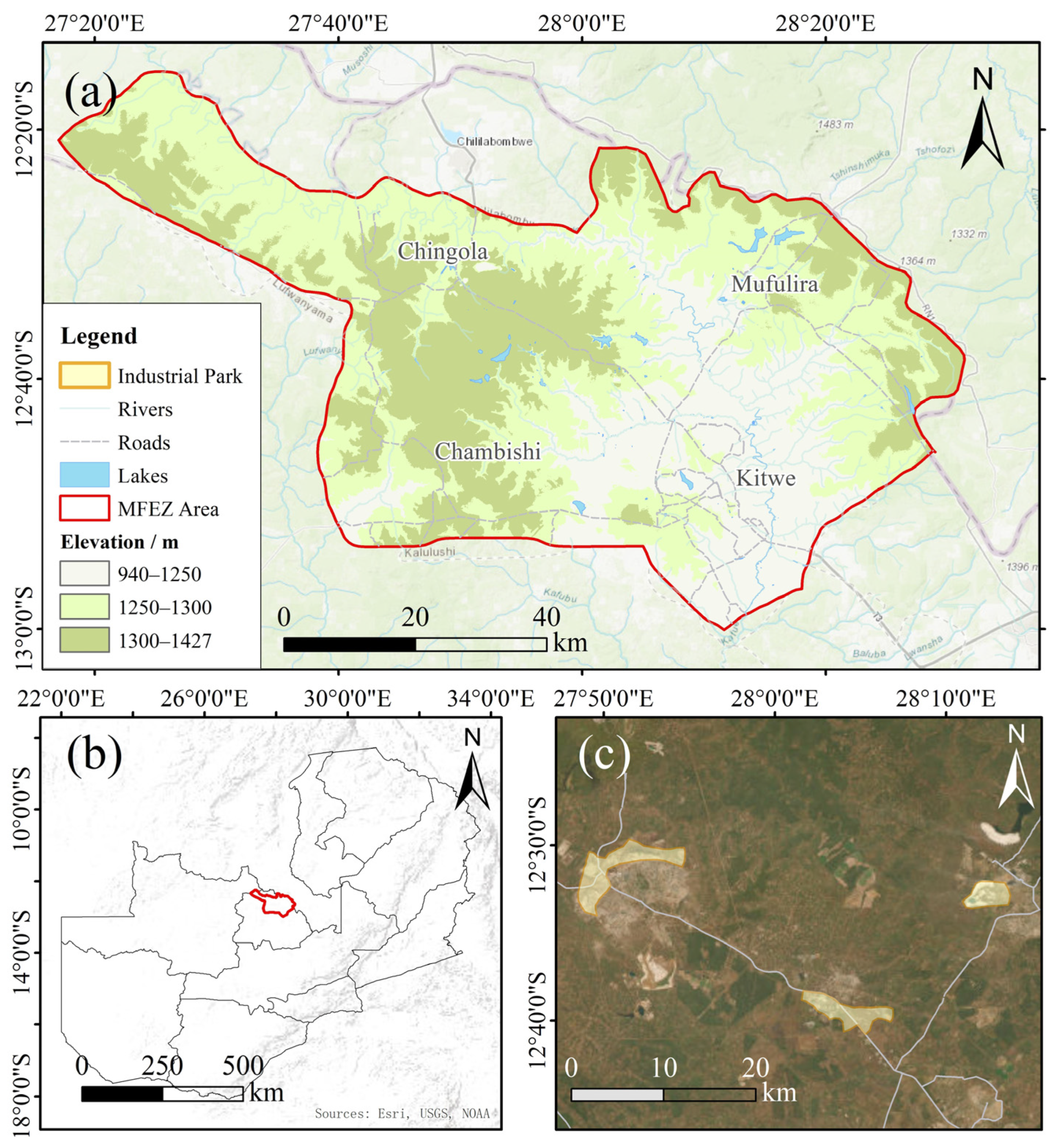
2.1. Research Area

This research concerns the Chambishi Multi-Facility Economic Zone (MFEZ) and its surrounding cities in Zambia as a case study for spatial–temporal analysis and quantification of the process of urban growth toward the achievement of SDG 11.3.1. The Chambishi MFEZ was established at the end of 2006 as one of the earliest China–Africa industrial cooperation zones, and served as the nation’s mining and industrial hub.

The research area includes four districts around the MFEZ: these are Chambishi, Kitwe, Chingola, and Mufulira. The research area is situated in the northern part of the Copperbelt Province, with latitude and longitude ranging from 27°16′–28°31′E to 12°14′–12°59′S (Figure 1). The climate of MFEZ is savannah type with an average annual temperature of 19.2 °C. The annual rainfall is about 1400 mm and the wet season is from December to April. Based on the 2022-Census-of-Population-and-Housing-Preliminary by Zambia Statistics Agency, the population growth rate of MFEZ was 4.5% in the period 2010–2020, above the 2.8% rate from 2000 to 2010.

2.2. Data Sources and Preprocessing

(1)

Landsat image dataset

Landsat imagery data from three specific years, 2000, 2010, and 2020, were selected for this study. Each image underwent preprocessing, and land-use classification was performed using the Random Forest method under the environment of the Google Earth Engine (GEE) platform. This classification divided the land into five categories: built-up land, forests, grassland, bare or cultivated land, and water area. The generated land-use data served as the dataset for further land-use simulations. Additionally, the original images assisted in extracting urban boundaries from nighttime light images, thereby verifying the accuracy of urban built-up area extraction.

(2)

Nighttime light (NTL) data

The VIIRS Black Marble nighttime lights dataset and the DMSP-OLS yearly data package, generated by NASA and NOAA (https://ngdc.noaa.gov/eog/download.html, accessed on 5 March 2024), were used for this research. These pre-processed nighttime light products eliminate the effects of noise and radiation, ensuring comparability across multiple years. The DMSP-OLS annual mean imagery for 2000, 2005, and 2010, along with VIIRS annual mean imagery for 2015 and 2020, was used in this study.

(3)

Additional geospatial data

The high-resolution spatial population grid data (1000 m) was downloaded from the WorldPop dataset (https://www.worldpop.org/, accessed on 5 March 2024), with adjustments made using officially published statistical yearbook data to serve as socioeconomic factors for the CA simulation analysis. DEM data, slope data, and river of the research area were obtained from the GEE platform and used as natural factors for the CA simulation analysis. Industrial park boundary data are sourced from the Belt and Road Initiative website (https://www.yidaiyilu.gov.cn/, accessed on 5 March 2024), while roads and railway track data were sourced from OpenStreetMap (https://www.openstreetmap.org/, accessed on 5 March 2024).

The types of geospatial and remote sensing data used in this research are listed in

Table 1. Summary of geospatial and remote sensing data.

Data	Description	Year	Source	Data Format
Landsat images	LULC Classification	2000 2010 2020	Google Earth Engine (GEE) (https://earthengine.google.com/, accessed on 5 March 2024)	GeoTIFF
nighttime light data	DMSP-OLS images	2000–2013	NOAA/NGDC (https://ngdc.noaa.gov/eog/download.html, accessed on 5 March 2024)	GeoTIFF
nighttime light data	NPP-VIIRS images	2013–2020	NOAA/NGDC (https://ngdc.noaa.gov/eog/download.html, accessed on 5 March 2024)	GeoTIFF
Population grid	Chambishi Mufulira Kitwe Chingola	2000 2010 2020	WorldPop (https://www.worldpop.org/, accessed on 5 March 2024)	GeoTIFF
Driving factors	DEM Slope River Railway Primary road	2020	Google Earth Engine (GEE) (https://earthengine.google.com/, accessed on 5 March 2024) And Open Street Map(OSM) (https://www.openstreetmap.org/, accessed on 5 March 2024)	GeoTIFF Shapefile KML

.

3. Methods

This research work is organized into three sections as shown in Figure 2. Therefore, utilizing NTL data from various years, the thresholding approach employing pseudo-invariant features (PIFs) was used in this study to identify urban built-up areas. The spatial pattern changes in urban areas were then analyzed by calculating the urban expansion index and standard deviation ellipse. Then, the spatial cooperative simulation approach based on the cellular automata was used to simulate the multifactor spatial coordination of LULC and population changes in 2030 under both natural and SDG scenarios. Lastly, the changes in the urbanization trends and urban land consumption patterns in the study area were examined by estimating the dynamics of the SDG 11.3.1 indicators in each year.

3.1. Urban Expansion Analysis Using NTL

3.1.1. Threshold Determination with PIFs Method

The urban built-up area has the fundamental data that need to be measured to assess SDG 11, and the expansion of the urban boundary is a visual representation of urban growth. Earlier research has demonstrated that nighttime light (NTL) images such as DMSP-OLS and VIIRS are useful data sources for monitoring urban boundaries [24]. However, there is no on-board calibration for DMSP satellites, which results in the difficulty of comparing data among different sensors in the same year and among the same sensor but different years [25]. Pseudo-invariant features (PIFs) are characteristics of urban regions. In mature urban areas, their NTL intensity levels remain consistently stable over a specific timeframe. These urban features are called “pseudo-invariant” because they have minimal fluctuations in NTL intensity [26]. In order to determine the optimal thresholds for each area, the NTL images may be divided into multiple parts with the use of PIFs. Subsequently, these parts can be divided into the built-up and unbuilt-up zones of the city, enabling accurate boundary identification. The approach for the identification of urban boundaries in this research is accomplished through the following steps:

First, all remote sensing images were preprocessed, and image mosaicking, clipping, reprojection, and resampling were performed on Envi 5.6 and ArcGIS 10.8 to ensure that the spatial resolution, coordinate system, and spatial extent of the images were consistent. The built-up area of the base year was used as an auxiliary baseline with the TM image of the year 2000. Binary iterations were applied to divide the NTL image into built-up and non-built-up areas according to Equation (1), and the optimal threshold for segmenting the built-up areas in the NTL image for the study area was obtained by iteratively testing various possible thresholds to minimize the Error:

$$\sum _{i=1}^n\left|{\widehat{A}}_{T,i}-A_i\right|=min$$

(1)

where $A_i$ denotes the actual built-up area derived from high-resolution TM image data, ${\widehat{A}}_{T,i}$ denotes the threshold-adjusted NTL data.

Subsequently, the PIFs zones were also identified for both the baseline and goal years. Saturated value pixels were excluded to create desaturated PIFs to ensure temporal stability. Based on the linear regression as in Equation (2), a correlation was done between the baseline year’s and the target year’s DN values.

$$PIF{s}_t=a\times PI{F}_{s_0}+b$$

(2)

where $a$ and $b$ denote the regression coefficients, $PI{F}_{s_0}$ is the DN value of the $PIFs$ region for the baseline year, and $PIF{s}_t$ denotes the DN value of the $PIFs$ region of the corresponding pixel in year $t$.

Thus, Equation (1) is used to calculate the most suitable reference threshold for the extraction of the built-up area of the city, and then by combining the same with Equation (3), the most suitable threshold for the extraction of the built-up area of the city in year $t$ is predicted, and hence the built-up area of the study area in each year is obtained based on this threshold [27].

$$Threshold{s}_t=m\times Threshold{s}_{2000}+n$$

(3)

where $m$ and $n$ denote the regression coefficients. $Threshold{s}_{2010}$ and $Threshold{s}_t$ denotes the ideal threshold for urban built-up areas in the baseline year and target year, respectively.

3.1.2. Urban Growth Indicators

Two indicators were computed: the Urban Land Expansion Difference Index (UEDI) and the Urban Land Expansion Intensity Index (UEI) for evaluating the geographical features of urban expansion with respect to the SDG context. The Urban Land Expansion Intensity Index (UEI) measures the rate at which urban land area expands over a specific period [28]. Once standardized, urban expansion rates across different time frames and spatial units become comparable. The UEI index is defined as Equation (4):

$$UE{I}_i={\displaystyle \frac{U{A}_i^{i+m}-U{A}_i^t}{U{A}_i^t\times m}}$$

(4)

where $UE{I}_i$ represents the urban land expansion intensity, $U{A}_i^{i+m}$ and $U{A}_i^t$ represent the urban land area in the spatial unit $\mathrm{i}$ of $t+m$ years, while $m$ is the total amount of years.

The relationship between the growth rates of the urban built-up areas in the research area and the corresponding general urban land use is defined by the Urban Land Expansion Difference Index (UEDI). UEDI provides a way to quantify the rate of urban land expansion inside different cities and has the ability to declare the degree of development to be irrelevant. The degree of development connections between the cities may also be determined by the index. Equation (5) defines this index:

$$UED{I}_i={\displaystyle \frac{\left|U{A}_i^{t+m}-U{A}_i^t\right|\times U{A}^t}{\left|U{A}^{t+m}-U{A}^t\right|\times U{A}_i^t}}$$

(5)

where $UED{I}_i$ represents the urban land expansion difference index, $U{A}^{t+m}$ represent the overall area of SEZs in $t+m$ years, m is the number of years in the study period.

The analysis of spatial patterns and variations in urban growth employed the Standard Deviation Ellipse (SDE) indicator [29]. This tool employs statistical analyses to explore the spatial distribution patterns of geographical elements, helping to establish the direction and scale of urban built-up area expansion [30]. The long and short axes of the ellipse represent the range and primary direction of the urban built-up areas, respectively, while the center of the ellipse represents the urban center. Equations (6)–(8) were utilized to calculate the Parameters of SDE.

The center of gravity $\left({\overline{X}}_w,{\overline{Y}}_w\right)$ of the standard deviation ellipse is:

$${\overline{X}}_w={\displaystyle \frac{{\sum }_{i=1}^n{w}_i{x}_i}{{\sum }_{i=1}^n{w}_i}}, {\overline{Y}}_w={\displaystyle \frac{{\sum }_{i=1}^n{w}_i{y}_i}{{\sum }_{i=1}^n{w}_i}}$$

(6)

The azimuthal $\alpha$ is

$$\begin{array}{c}\mathit{tan}\alpha ={\displaystyle \frac{{\sum }_{i=1}^n{\omega }_i^2{\tilde{x}}_i^2-{\sum }_{i=1}^n{w}_i^2{\tilde{y}}_i^2}{2{\sum }_{i=1}^n{w}_i^2{\tilde{x}}_i{\tilde{y}}_i}}\\ +{\displaystyle \frac{\sqrt{{\left({\sum }_{i=1}^n{w}_i^2{\tilde{x}}_i^2-{\sum }_{i=1}^n{w}_i^2{\tilde{y}}_i^2\right)}^2+4{\sum }_{i=1}^n{w}_i^2{\tilde{x}}_i^2{\tilde{y}}_i^2}}{2{\sum }_{i=1}^n{w}_i^2{\tilde{x}}_i{\tilde{y}}_i}}\end{array}$$

(7)

The standard deviation ${\sigma }_x$ of the x-axis and the standard deviation ${\sigma }_y$ of the y-axis are:

$$\begin{array}{c}{\sigma }_x=\sqrt{{\displaystyle \frac{{\sum }_{i=1}^n{\left(w_i{\tilde{x}}_i\mathit{cos}\alpha -w_i{\tilde{y}}_i\mathit{sin}\alpha \right)}^2}{{\sum }_{i=1}^n{w}_i^2}}},\\ {\sigma }_y=\sqrt{{\displaystyle \frac{{\sum }_{i=1}^n{\left(w_i{\tilde{x}}_i\mathit{sin}\alpha -w_i{\tilde{y}}_i\mathit{cos}\alpha \right)}^2}{{\sum }_{i=1}^n{w}_i^2}}}\end{array}$$

(8)

where $\left(x_i,y_i\right)$ denotes the spatial location of the research object, $w_i$ denotes the corresponding weight, and $\left({\tilde{x}}_i,{\tilde{y}}_i\right)$ denotes the coordinate deviation of the location of each research object to the center of gravity $\left({\overline{X}}_w,{\overline{Y}}_w\right)$.

3.2. Simulation of Land-Use and Population Changes

The Spatial Cooperative Simulation (SCS) approach was developed by Professor Tu Wei of Shenzhen University and used to model synergistic changes in multiple spatial elements such as land use, population, and economy under the synergistic influence of natural and human factors [31]. This methodology enhances the traditional urban Cellular Automata (CA) model by integrating the simultaneous development processes of various spatial attributes, which can be divided into two primary parts. The two are the initial simulation and the step-wise cooperative simulation. The first part of the simulation employs the normal CA-based feature simulation (CAFS) to explain the spatial transformations of land use, population, and economic criteria. The step-wise cooperative simulation part follows CAFS and delves into how these spatial components influence one another and, based on the preceding iteration’s results, refine the simulation outcomes incrementally. This iterative refinement process is designed to capture the nuanced co-evolutionary patterns among land use and population growth offering a robust framework for forecasting urban expansion and its social factors.

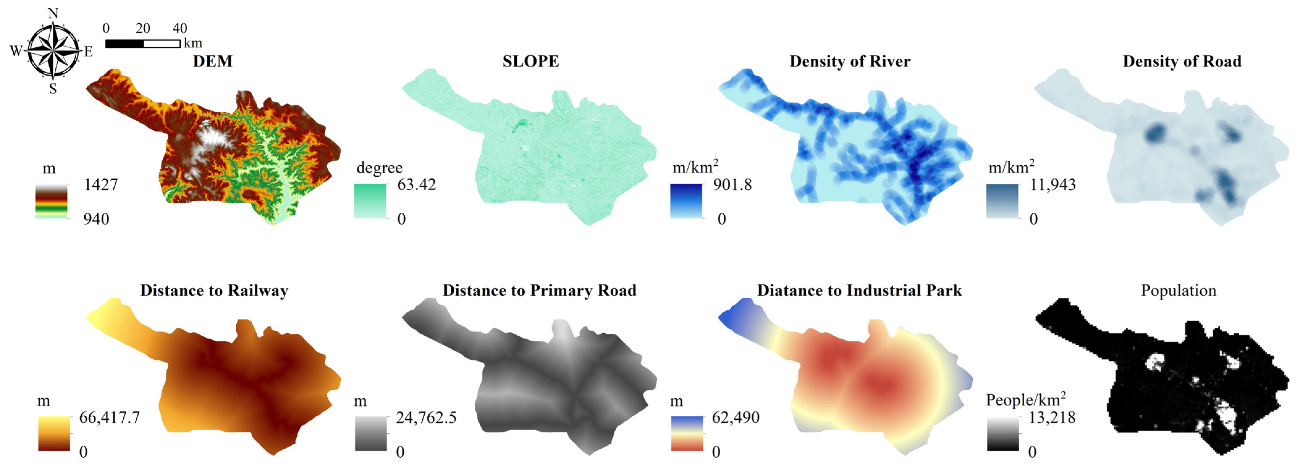
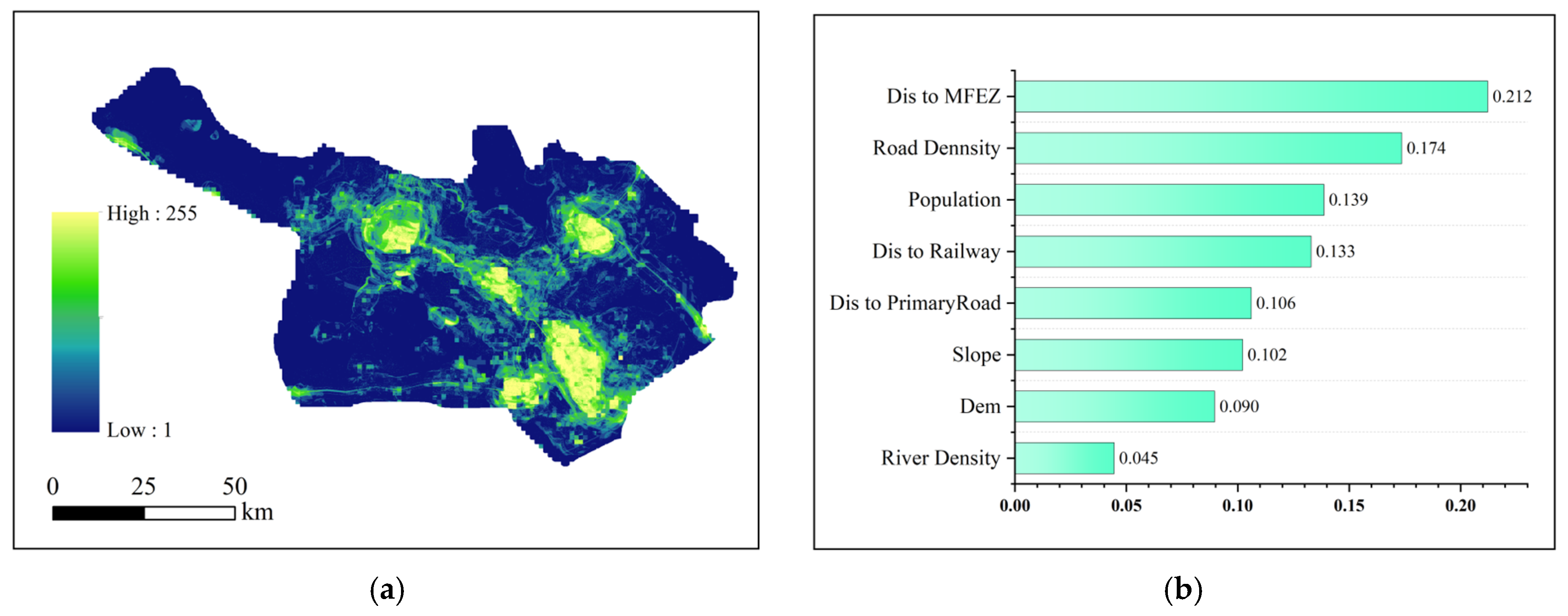
3.2.1. Driving Factors of Land Use and Population

Land-use and population changes are influenced by the natural environment, transportation, and geographical location [32,33]. In order to comprehensively identify the drivers of LU and POP change in the study area, binary images of land-use types with hierarchical images of population grids were used as the dependent variable, and the independent variable was the tested driving factors. Logistic regression equations were used to assess the probability of different drivers, with their accuracy verified by the relative operating characteristic (ROC). A ROC value greater than 0.7 signifies that the logistic regression equation is valid. Three categories totaling 12 drivers were selected for validation based on the geographic characteristics of the study area, including natural factors (elevation, slope, aspect, temperature, and density of river), social factors (NTL density, population density, distance to railways, distance to primary road and secondary road), and locational factors (distance to industrial park and distance to district center).

After calculation, there are 8 drivers with ROC values greater than 0.7, which are topography, slope, DEM, river density, road density, distance to railways, distance to primary road, distance to industrial parks, and population density. The above eight driving factors have a good correlation with LU and POP change in MFEZ, which meets the requirements and can be applied in the subsequent model [34] (Figure 3).

3.2.2. CA-Based Feature Simulation

The base layer of the SCS approach is CA-based feature simulation (CAFS). This study employed the PLUS model for CA-based feature simulation, PLUS model is a raster data-based predictive simulation CA model. The system can model the interconnections between the spatial factors and it can also determine the causes of the spatial elements’ changes during the simulation. The PLUS model consists of two main modules: a rule mining framework that employs a model known as Land Expansion Analysis Strategy (LEAS), and a CA model based on the Multi-Type Stochastic Plate Seed (CARS) [20].

LEAS module is used to sample the expansion part of each type of LULC change in the two periods for training and Random Forest is used to model the factors that influence the expansion and driving factors of each type of LULC change in order to obtain the probability of the expansion of each type of LULC and the contribution of the driving factors to the expansion of each type of LULC in that time period, and the formulae are shown in Equation (9), the development probability $P_{gdu,k}\left(x\right)$, for a spatial unit $u$ transitioning to a specific feature state $k$:

$$P_{gdu,k}\left(x\right)={\displaystyle \frac{1}{M}}\sum _{m=1}^{M}I\left(h_m\left(x\right)=d\right)$$

(9)

where $x$ represents the vector of driving factors, $M$ the total number of decision trees within the Random Forest model, $I$ the indicator function, and $d$ denotes the desired feature state.

The CARS module combines the stochastic seed selection and a threshold reduction technique to automatically generate simulated patches while meeting development probability constraints as described by Equation (10):

$${OP}_{i,k}^{d=1,t}=P_{i,k\left(X\right)}^d\times {\mathsf{\Omega }}_{i,k}^t\times D_k^t$$

(10)

where ${OP}_{i,k}^{d=1,t}$ is the combined probability of a shift in land-use type to $k$ at spatial cell $i$; $P_{i,k\left(X\right)}^d$ denotes the probability of growth of the land-use type in cell $i$; $D_k^t$ is the effect of the future demand for the land-use type $k$, which is an adaptive driving coefficient depending on the difference between the amount of land available at the current iteration $t$ and the targeted demand difference; ${\mathsf{\Omega }}_{i,k}^t$ denotes the neighborhood effect of cell $i$, which is the proportion of the land-use component of $k$ that is covered in the following neighborhood.

3.2.3. Initial and Step-Wise Cooperative Simulation with CAFS

To ensure the consistency and clarity of subsequent complex simulations within the CA framework, population data were first converted into categorical variables. Given the positively skewed distribution of the population data, the natural breaks method was employed to maximize inter-group variance and minimize intra-group variance [35].

Initial simulations were conducted using these driving factors along with categorical features. The LU CAFS and POP CAFS were implemented separately, resulting in the initial simulation outcomes of IS-LU and IS-POP at the current time t.

At the heart of the SCS approach, there is the Step-wise Cooperative Simulation process. In this case, the initial results of the simulation are used as inputs to the following simulation rounds. This iterative process allows for the modeling of complex interactions and dependencies among land-use and population variables, capturing the co-evolution of these features over time.

The iterative update formula can be represented as Equation (11), where $S{C}_{Lt+1}^n$ and $S{C}_{Pt+1}^n$ denote the simulated land-use and population output at iteration $n$ for time $t+1:$

$$\begin{array}{l}S{C}_{Lt+1}^n=f_L\left(S{C}_{Pt}^{n-1},S{C}_{Lt}^{n-1},X_t\right)\\ S{C}_{Pt+1}^n=f_P\left(S{C}_{Lt}^{n-1},S{C}_{Pt}^{n-1},X_t\right)\end{array}$$

(11)

where $f_L$ and $f_P$ represent the CA models for land use and population, respectively, and $X_t$ encompasses the spatial variables at time $t$. This formulation ensures that the simulation dynamically incorporates the evolving states of each spatial feature.

3.3. Accuracy Validation

For the assessment of accuracy, four indicators were respectively used. To assess the accuracy of Pseudo-Invariant Features (PIFs) in extracting built-up areas, Overall Accuracy (OA) was utilized. OA measures the proportion of correctly classified cells in relation to the total number of cells in the research area [36]; it is calculated using Equation (12):

$$OA=1-{\displaystyle \frac{A+B+X}{N}}$$

(12)

where $N$ represents the total number of cells in the research area. $A$ is the area where changes are incorrectly simulated as unchanged, $B$ is the correctly simulated changes, and $X$ is the area where changes are incorrectly categorized.

The performance of the land-use simulation was further assessed using the figure of Merit (FoM), which evaluates the accuracy of change detection by considering both correctly and incorrectly simulated areas [37]. The FoM is defined as Equation (13):

$$FOM={\displaystyle \frac{B}{A+B+X+Y}}$$

(13)

$Y$ is the area where unchanged regions are incorrectly simulated as changed.

For population simulations, the Root Mean Square Error (RMSE) was employed to quantify the difference between real and simulated populations [38]. RMSE can be defined as Equation (14):

$$RMSE=\sqrt{{\displaystyle \frac{{\Sigma }_{i=1}^M{\left(v_{i,t}-v_{i,t}^{\prime }\right)}^2}{M}}}$$

(14)

where $M$ represents the number of spatial units within the research area. The term $v_{i,t}$ refers to the observed feature value density in sub-district $i$ at time $t$, while $v_{i,t}^{\prime }$ denotes the simulated feature value density in sub-district $i$ at the same time.

3.4. Spatiotemporal Assessment of SDG 11.3.1 Indicator

Within the UN-Habitat Sustainable Development Goal (SDG) 11 indicators, indicator 11.3.1 means ‘urbanization trends and urban land consumption patterns’. This indicator quantitatively evaluates the relationship between urban population expansion and urban land growth through the ratio of land consumption rate to population growth rate (LCRPGR) [2]. The indicator also has the limitation that it does not capture the impact of social and environmental policies on land-use efficiency. However, the indicator is still a key indicator for tracking progress toward sustainable urbanization by providing a unified monitoring of urbanization trends and urban land consumption patterns from the perspective of the urban habitat, from the local urban scale to the regional and global scales.

SDG 11.3.1 indicator was used in this study to track population increase and urban land expansion inside the urban boundaries of the research area [39]. The 2000, 2010, and 2020 urban boundaries are the urban built-up area extracted by the PIFs method, while for 2030, the simulated built-up land pixels are selected as the urban built-up area. Next, the values of the SDG 11.3.1 indicators were computed based on changes in population and urban land use inside this area. The following Equation (15) was used to calculate the land consumption rate (LCR), the population growth rate (PGR), and the ratio of the land consumption rate to the population growth rate (LCRPGR):

$$\left\{\begin{array}{c}PGR={\displaystyle \frac{\mathit{ln}\left(P{op}_{t+n}/{Pop}_t\right)}{n}}\\ LCR={\displaystyle \frac{\mathit{ln}\left(U{rb}_{t+n}/{Urb}_t\right)}{n}}\\ LCRPGR={\displaystyle \frac{LCR}{PGR}}\end{array}\right.$$

(15)

where ${Pop}_t$ represents the population in year $t$, $P{op}_{t+n}$ represents the population in year $t+n$, ${Urb}_t$ is the area of built-up land in year $t$, and $U{rb}_{t+n}$ is the area of built-up land in year $t+n$. In an ideal scenario, the ratio of land consumption to population growth would be 1, indicating that urban land expansion matches the pace of population growth. Grids can be classified into five categories according to their LCRPGR values, as illustrated in

Table 2. LCRPGR Value Categories and Meaning.

LCRPGR Value	Meaning
LCRPGR < −1	the rate of population decline is greater than the rate of built-up area expansion
−1 < LCRPGR ≤ 0	the rate of population decline is less than the rate of built-up area expansion
0 < LCRPGR ≤ 1	the rate of population growth is greater than the rate of built-up area expansion
1 < LCRPGR ≤ 2	the rate of built-up area expansion is 1–2 times the rate of population growth
LCRPGR ≤ 2	the rate of built-up area expansion is greater than 2 times the rate of population growth

.

Historical LULC data and WorldPop population data were used to calculate PGR, LCR, and LCRPGR for the years 2000, 2010, 2020, and 2030. These calculations were performed in kilometer grids using the SCS approach for land use and population. The results were then mapped to more effectively illustrate the spatial and temporal changes.

4. Results

4.1. Spatial and Temporal Changes in Urban Expansion

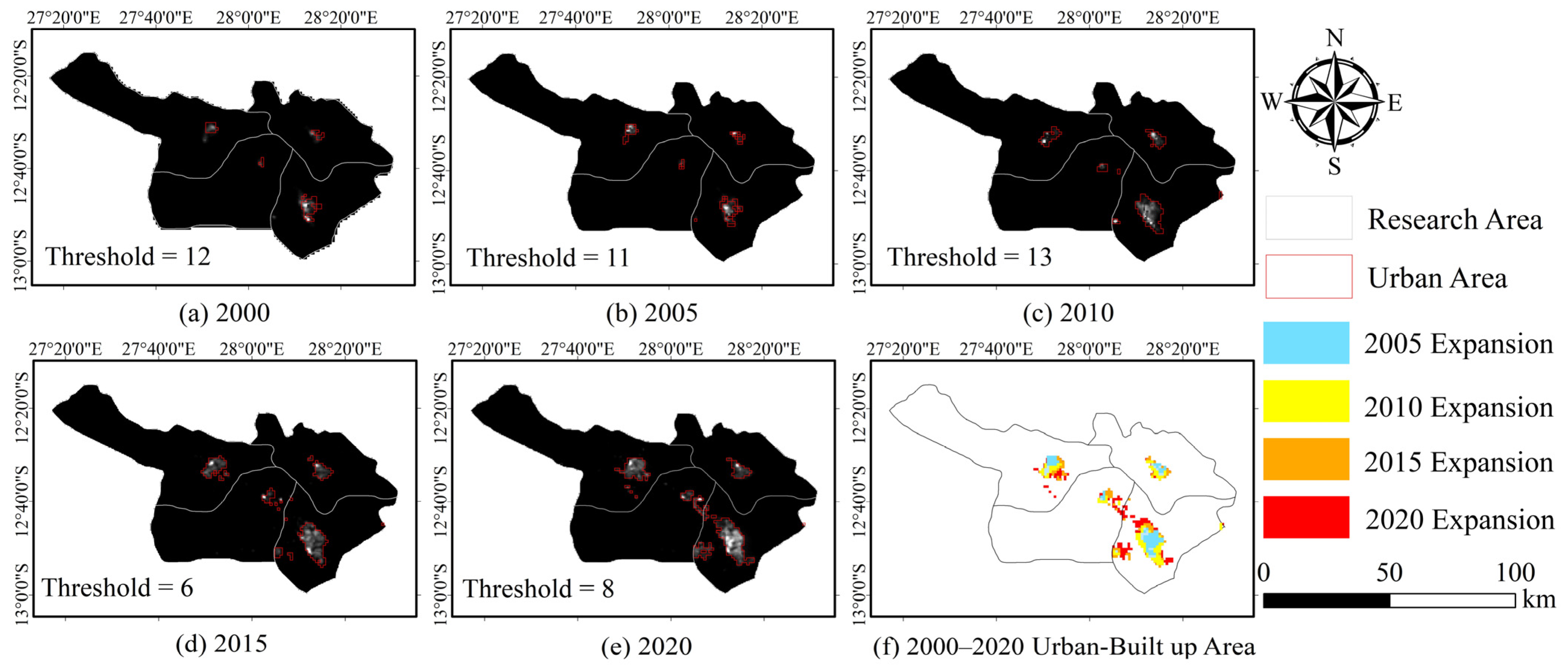
4.1.1. Extracting Urban Built-Up Area from NTL Images Using PIFs Method

The PIFs method and the baseline year’s high-resolution Landsat images were used to determine the urban built-up areas nighttime light thresholds for the years 2000, 2005, 2010, 2015, and 2020, which were found to be 12, 11, 13, 6, and 8, respectively. To compare the results of the PIFs method, the Simple Threshold Segmentation (STS) method based on a single year was also used to extract the urban built-up areas for the years 2000, 2005, and 2010. Multiple thresholds were tested, and a threshold of 12 was ultimately chosen to extract the urban areas for the mentioned years (Figure 4).

Using visual interpretation of Google Map satellite images, 250 randomly selected points within the study area were manually classified as either ‘urban area’ or ‘non-urban area’ to validate overall accuracy (OA). After performing the validation calculations, the lowest OA value obtained by the PIFs method for the urban built-up area over five years was 84.6%, with an average OA of 86.7%. This is notably higher than the 80.7% average OA achieved by the STS method (

Table 3. Accuracy validation of the PIFs Method and STS Method.

Method	Year	Overall Accuracy (OA)
PIFs	2000	0.883
	2005	0.931
	2010	0.846
	2015	0.865
	2020	0.876
STS	2000	0.883
	2005	0.721
	2010	0.817

). These findings indicate that the PIFs method is reliable and meets the requirements for subsequent studies.

The built-up area of the four districts in the MFEZ was extracted (Figure 5), and it can be seen that the individual districts’ urban built-up areas are mainly located in the center of the MFEZ. Through the experimental results, it was found that urban land has continued to increase throughout the MFEZ, and urban development has shown an expansion trend, but the rate of expansion of cities within the MFEZ is not balanced in time and space (Figure 6).

Between 2000 and 2020, the built-up areas of all four cities in the MFEZ expanded significantly. Kitwe showed the largest increase, growing from 51.21 km² to 164.89 km². Chambishi, starting with the smallest area, exhibited the fastest growth, increasing from 3.07 km² to 30.72 km². Chingola and Mufulira also experienced notable expansion, with Chingola’s built-up area growing from 19.46 km² to 58.38 km² and Mufulira’s from 13.31 km² to 36.87 km².

The overall trend in the MFEZ is consistent, with each of its cities showing distinctive development. Chambishi, located centrally within the MFEZ, exhibited the highest expansion rate among all cities, with a remarkable increase of over 900% from 2000 to 2020. Kitwe, as the center city of the region, followed with an expansion rate exceeding 222%, while Chingola and Mufulira showed comparatively lower rates of expansion. The analysis of spatial and temporal changes in urban expansion within the MFEZ shows significant growth in built-up areas across all cities, with Chambishi having the highest growth rates and intensity. The data highlight the uneven situation of urban expansion, driven by industrial activities, particularly in Chambishi and Kitwe.

4.1.2. Calculation of the Spatial and Temporal Change Index for Urban Expansion

The situation of urban development in the region has changed rapidly because the construction of the MFEZ has dramatically altered urban planning and land-use management, which can be seen from the changes in the UEI and UEDI in

Table 4. Urban Expansion Index.

	Period	Chingola	Chambishi	Kitwe	Mufulira
UEI	2000–2005	0.021	0.133	0.020	0.031
	2005–2010	0.114	0.320	0.200	0.227
	2010–2015	0.133	0.154	0.038	0.013
	2015–2020	0.007	0.061	0.046	0.012
	2000–2020	0.100	0.450	0.111	0.088
UEDI	2000–2005	0.813	5.152	0.773	1.189
	2005–2010	0.596	1.670	1.043	1.183
	2010–2015	2.279	2.629	0.653	0.214
	2015–2020	0.216	1.804	1.357	0.349
	2000–2020	0.854	3.844	0.948	0.756

. It can be observed that Chingola’s UEI increased from 0.021 (2000–2005) to 0.133 (2010–2015) and then significantly decreased to 0.007 (2015–2020). Chambishi’s UEI started high at 0.133 (2000–2005), peaked at 0.320 (2005–2010), and showed a slight decrease to 0.061 (2015–2020). Kitwe’s UEI showed an increase from 0.020 (2000–2005) to 0.200 (2005–2010), then a decrease to 0.038 (2010–2015), and a subsequent rise to 0.0458 (2015–2020). Mufulira’s UEI increased from 0.031 (2000–2005) to 0.227 (2005–2010), then dropped to 0.013 (2010–2015) and further decreased slightly to 0.012 (2015–2020). These changes reflect the impact of the MFEZ on urban expansion, highlighting the varying rates and intensities of development in different districts over time.

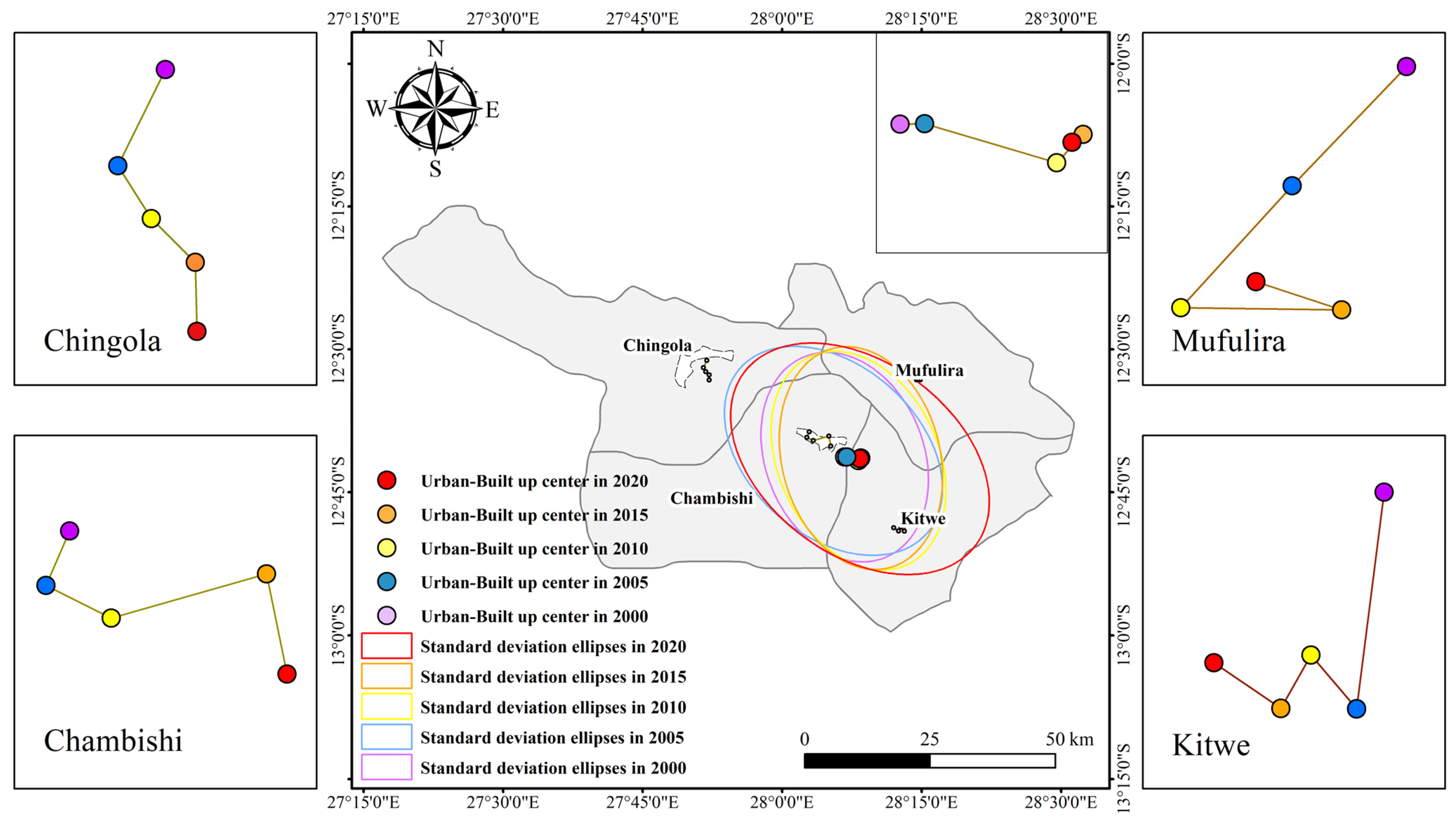
4.1.3. Characterization of Urban Expansion Standard Deviation Ellipse (SDE)

The MFEZ’s standard deviation ellipse of urban expansion was calculated using the extracted urban built-up area boundaries for each year. This enabled the demonstration of the overall pattern and extent of the urban agglomeration’s expansion. The standard deviation ellipse of the urban agglomeration gradually expands, especially between 2005–2010 and 2015–2020, the ellipse area increases significantly, indicating that the urban area’s expansion speed is accelerated in this period (Figure 7). At the same time, the shape and direction of the standard deviation ellipse change in a certain direction, mainly expanding in the southeast direction, which indicates that the expansion of the city has an obvious directionality, the same as the region where the industrial park and regional center city is located.

At the same time, this work estimates the path of migration of the center point of the urban agglomeration, which depicts the process of urban expansion. The center point and the standard deviation ellipse as well as their expansion direction are also consistent, and both of them shift to the southeast or east direction with the change of years. Thus, the further development of the city cluster is mainly directed toward the southeast, which allows stating that the construction of infrastructure and economic activities in this direction is more active.

The migration of the centroids in the four cities highlights each city’s individual contribution to overall expansion. The centroids of Chingola and Chambishi gradually shifted southward, indicating that their expansion was influenced by the southern region. In contrast, the centroids of Mufulira and Kitwe remained relatively stable, displaying a more uniform expansion without clear directionality. This pattern could be influenced by early urban planning and construction strategies in these cities. The direction and speed of expansion vary from city to city but are generally consistent with the overall expansion trend of the urban agglomeration.

4.2. Synergistic Land-Use Population Modeling

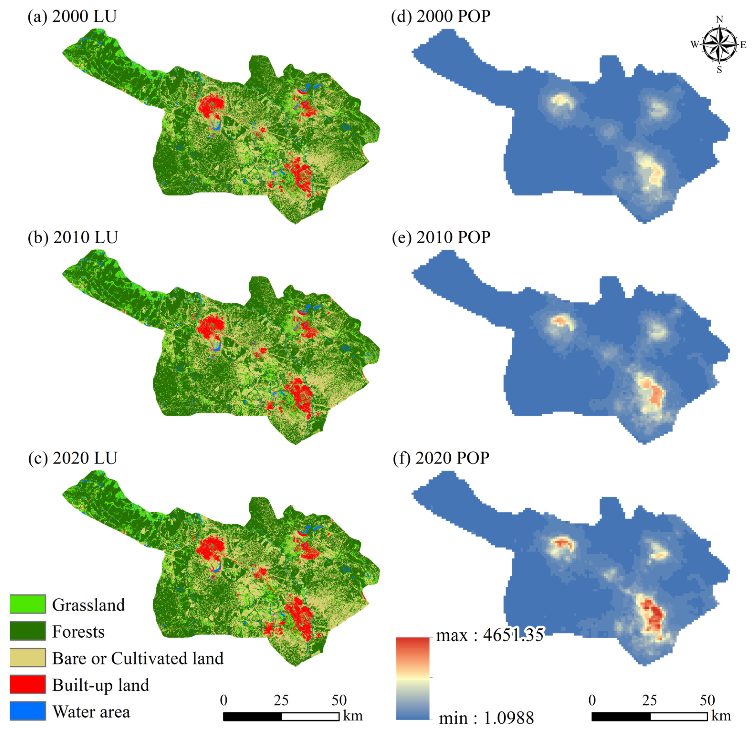
4.2.1. Temporal and Spatial Variation in Land Use and Population

The degree of land-use change and the spatial distribution of the population over the last two decades provide critical insights into urban environmental monitoring. Within the study region, there have been notable variations in both land use and population distribution, according to data gathered from the GEE platform. For the years 2000, 2010, and 2020, the classification’s overall accuracy (OA) was 87.1%, 88.5%, and 89.7%, respectively.

The quantity of land use in the research area increased significantly between 2000 and 2020 (Figure 8), with built-up areas increasing by nearly 55%, from 187.6 km² in 2000 to 289.7 km² in 2020 and grasslands by approximately 12%, indicating rapid urbanization and land transformation. Water areas decreased from 107.7 km² in 2000 to 94.7 km² in 2020, with reduction rates of −4.12% from 2000 to 2010 and −8.23% from 2010 to 2020, suggesting a substantial loss of water bodies. Forests saw a decline from 3091.8 km² to 2888.7 km², with negative change rates of −2.01% and −4.65% (

Table 5. Areal Changes in LULC Type in 2000–2020.

LULC Classes	Area (km2)			Change Rate (%)
	2000	2010	2020	2000–2010	2010–2020
Grassland	575.8	598.8	647.3	3.99	8.11
Forests	3091.8	3029.6	2888.7	−2.01	−4.65
Bare land and Cultivated land	1493.6	1499.6	1536.0	0.40	2.43
Built-up land	187.6	225.3	289.7	20.07	28.61
Water area	107.7	103.2	94.7	−4.12	−8.23

).

Population trends in the four districts also varied, with Chambishi exhibiting the fastest growth, nearly tripling in size, driven by an accelerating annual growth rate from 3.17% to 6.08%. Chingola and Kitwe saw substantial population increases, though Kitwe’s growth rate slowed as its population size grew. Mufulira experienced the steadiest growth, with modest increases in both population and growth rate (

Table 6. Population Changes in each District in 2000–2020.

Districts	Population			Annual Change Rate (%)
	2000	2010	2020	2000–2010	2010–2020
Chambishi	75,806	100,381	170,701	3.17	6.08
Chingola	172,026	216,602	299,936	2.59	3.68
Kitwe	376,124	517,543	661,901	3.61	2.77
Mufulira	143,930	162,889	200,182	1.38	2.32

).

Figure 9 presents the spatial distribution of land use and the population grid over three years. Built-up land is primarily concentrated in the centers of the four districts, with Bare or Cultivated land surrounding these areas, and forests and grasslands located further out. From 2000 to 2020, there was a significant increase in built-up land in the districts, which transformed surrounding bare or cultivated land and water areas, and some forests near the built-up land degraded into Bare or Cultivated land.

The population grid shows a sharp increase in the population of the urban center and a large increase in the spread of the population. Chambishi district has the most significant population growth, while other districts such as Kitwe and Chingola have slower population growth but also show a trend of gradual increase over time.

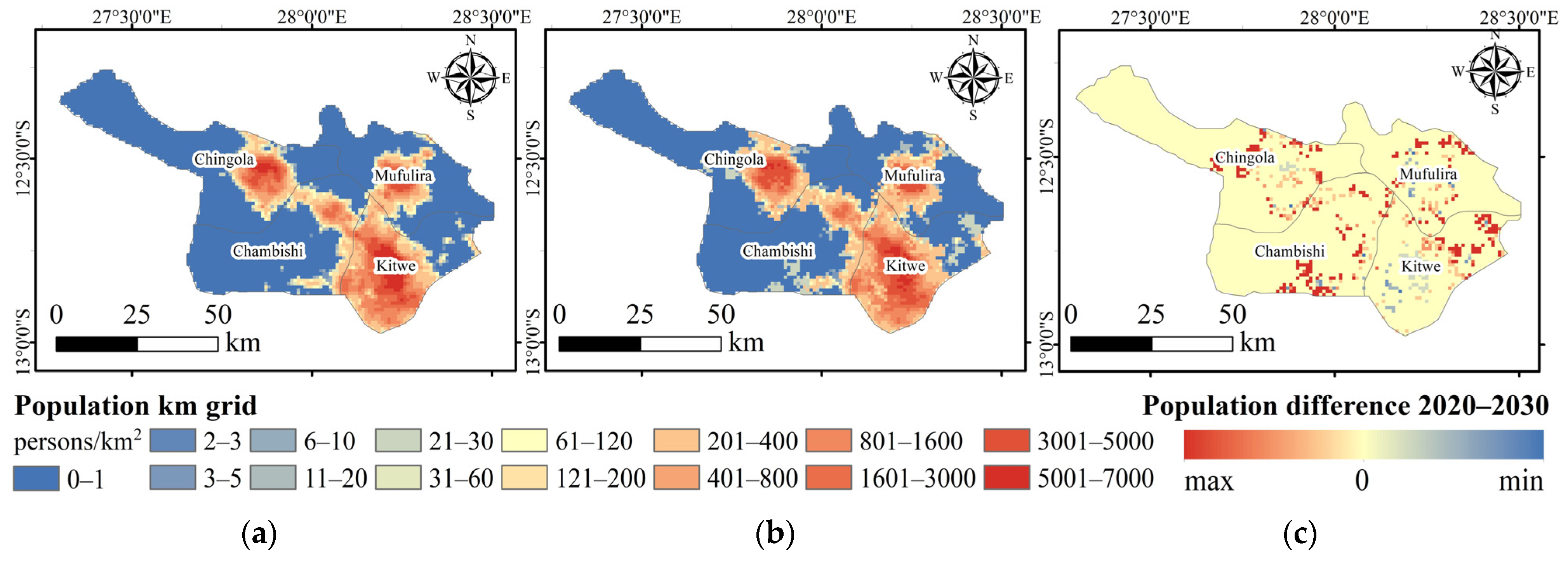
4.2.2. Spatial Cooperative Simulation of LULC-Population

This study simulated the land-use data and the population grid in 2020, calculated the overall accuracy (OA) and FoM index based on the real land-use data in 2020, and calculated the RMSE based on the real population grid data in 2020. The overall accuracy reached 92%; the software output of the FoM index was 0.12, which is in the range of 0.01 to 0.25; and the RMSE was 3.21, demonstrating that estimations of the population and land use in the research area can be made using the data and model employed.

The PLUS model within SCS is used for the identification of the land-use pattern of the research area in the year 2030, with two scenarios and modifications in the land-use demand, transfer probabilities, and constraints. The first is a natural development scenario in which land-use change is related only to historical land change characteristics. The driving factors of future land use are the same as the current status, which means a sprawling development without SDG 11.3 planning constraints. The second scenario is the SDG11.3 planning constraints that allow urban construction to match the population growth rate and sustainable development for humans and nature (Figure 10).

The natural development scenario without SDG planning constraints in 2030 is shown in Figure 10c and

Table 7. LULC Transfer Matrix for Natural Development Scenarios in 2020–2030 (unit: km²).

Land-Use Types	Grassland	Forests	Bare or Cultivated Land	Built-Up Land	Water Area	Total
Grassland	642.2	3.9	0.0	1.2	0.0	647.3
Forests	51.3	2663.7	27.3	118.7	27.6	2888.7
Bare or Cultivated land	0.0	0.0	1536.0	0.0	0.0	1536.0
Built-up land	0.0	0.0	0.0	289.7	0.0	289.7
Water area	0.0	0.0	0.4	0.0	94.4	94.7
Total	693.5	2667.6	1563.7	409.6	122.0	0.0

; there is a serious problem of encroachment of the built-up area on other land-use types in the study area, and the rapid expansion of towns and cities significantly affects the evolution of land-use patterns. Under this scenario, the urban built-up land around MFEZ will expand to 409.6 km² by 2030, an increase of 119.9 km², and a large number of forests and grassland are transformed into the built-up area and 51.3 km² of forests degraded to grassland, failing to achieve sustainable urban planning and management.

Under the sustainable development scenario in 2030 (Figure 10d and

Table 8. LULC Transfer Matrix for Sustainable Development Scenarios in 2020–2030 (unit: km²).

Land-Use Types	Grassland	Forests	Bare or Cultivated Land	Built-Up Land	Water Area	Total
Grassland	647.3	0.0	0.0	0.0	0.0	647.3
Forests	28.9	2699.4	152.3	8.0	0.1	2888.7
Bare or Cultivated land	17.3	58.2	1394.9	65.5	0.1	1536.0
Built-up land	0.0	0.0	0.0	289.7	0.0	289.7
Water area	0.0	0.0	7.5	0.1	87.2	94.7
Total	693.5	2757.6	1554.7	363.3	87.4	0.0

), the built-up area still expands to 363.3 km², but the expansion area decreases and closely follows the existing urban sprawl in spatial distribution. The pattern of degradation of forests is similar to that in the natural scenario, but the downward trend is slower than in the natural scenario, with the area transferred out decreasing from 221.1 km² to 131.1 km². Urban expansion in the sustainable development scenario is more orderly than in the natural development scenario, where the city’s infrastructure is better able to serve the newly added built-up area, contributing to a better habitat.

To obtain the simulation results of the population grid in 2020 under the sustainable development scenario, a spatial cooperative simulation approach was applied to the population grid data through synergistic development with land-use data; the results were compared (Figure 11), the population was counted into districts (

Table 9. Population changes in each district in 2020–2030.

Districts	Population		Annual Change Rate (%)
	2020	2030	2020–2030
Chambishi	170,701	267,686	4.60
Chingola	299,936	365,479	1.99
Kitwe	661,901	761,511	1.41
Mufulira	200,182	249,561	2.23

). The total population of these four districts as at 2030 was 1644,237; Chambishi district had the highest population increase of from 170,701 to 267,686. The results of the population simulation for the year 2030 were similar to the land-use simulation, and the main regions of population increase are concentrated on the edge of the built-up area. Moreover, the population within the cities of Chingola, Mufulira, and Kitwe was reduced, which could have been as a result of the depopulation of the big cities.

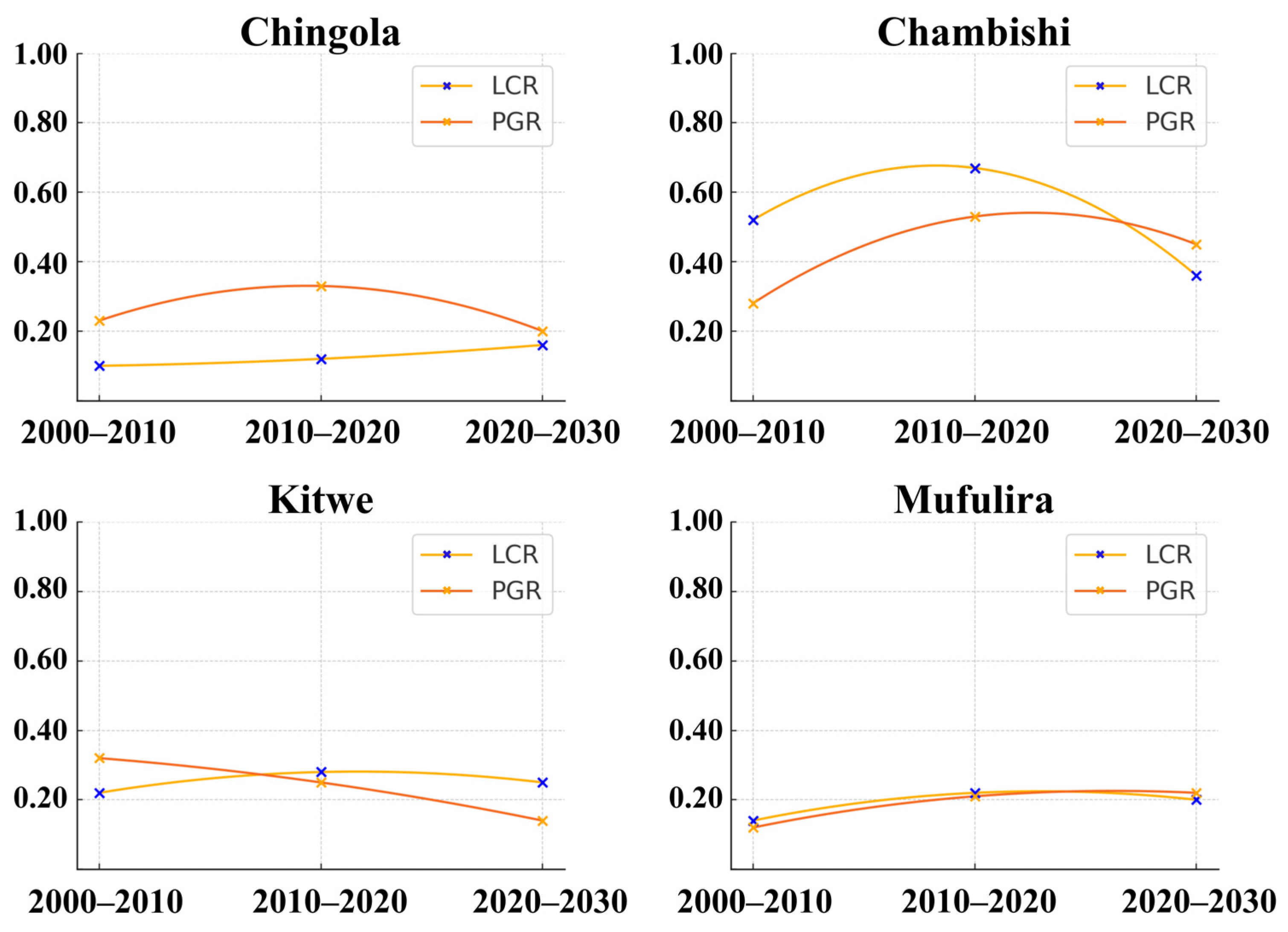
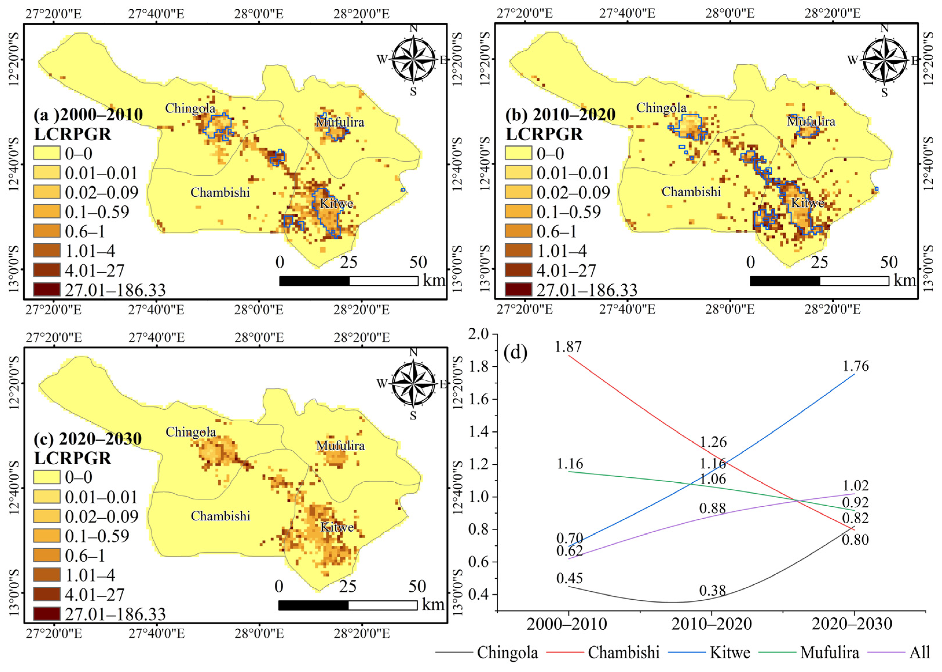
4.3. Spatiotemporal Variation in Land Consumption and Population Growth (SDG 11.3.1)

Based on the land-use classification results, the temporal variations in LCR, PGR, and LCRPGR indicators were measured in the study (

Table 10. LCR and PGR for each District for three time periods.

Districts	2000–2010			2010–2020			2020–2030
	LCR	PGR	LCRPGR	LCR	PGR	LCRPGR	LCR	PGR	LCRPGR
Chingola	0.10	0.23	0.45	0.12	0.33	0.38	0.16	0.20	0.82
Chambishi	0.52	0.28	1.87	0.67	0.53	1.26	0.36	0.45	0.80
Kitwe	0.22	0.32	0.70	0.28	0.25	1.16	0.25	0.14	1.76
Mufulira	0.14	0.12	1.16	0.22	0.21	1.06	0.20	0.22	0.92

). Chambishi and Kitwe show higher LCR, especially during the 2020–2030 period, where land-use growth begins to outpace population growth, which indicates a higher density of land development projects. Chingola and Mufulira show PGR that exceeds or is close to LCR for most of the period (Figure 12).

During the period 2000–2010, Chambishi had the least efficient urban sprawl with an LCRPGR of 1.87, while Chingola had the lowest LCRPGR (0.45) and the highest urbanization trends and urban land consumption patterns During the period 2010–2020, Chambishi’s LCRPGR has decreased significantly but was still larger than 1 (1.26), while Kitwe has experienced an increase in urban sprawl, from 0.70 in the previous period to 1.16. The simulation for the period 2020–2030 indicates that Chambishi and Mufulira’s urban land consumption patterns will continue to improve with LCRPGRs of 0.80 and 0.82, respectively, while Kitwe’s LCRPGR value continues to decrease rapidly, reaching 1.76 (Table 10).

Comparative analysis of the LCRPGR values for the three periods, using the kilometer grid and administrative districts as segmentation units, respectively, indicated different trends in urbanization trends and urban land consumption patterns in both time and space of the four districts, with the built-up area boundaries obtained using the PIFs method identifying the urban area. (Figure 13) It was observed that the LCRPGR values of the entire area have changed considerably over time as shown. The LCRPGR values of most of the units outside the urban area are in the range of (0, 0.01], and the areas with higher LCRPGR values are located within the urban area. During 2000–2010, it was observed that the urban perimeter of the four districts clusters many units with high LCRPGR values, indicating that these surrounding areas were behind the LCR in terms of PGR and were in the early stages of rapid urbanization [40]. This phenomenon was more serious in the period 2010–2020, showing a high degree of spatial heterogeneity throughout the study area, and the emergence of this phenomenon was closely related to the unplanned urban expansion of the MFEZ in Zambia. In Zambia, due to insufficient government involvement and land management, the MFEZ had less impact on spatial optimization and land values, and problems such as illegal occupation and inadequate spatial assessment have emerged [5]. Uncontrolled urban population expansion leads to sprawling slums and also leads to a lack of infrastructure. Applying the simulated population and land-use data in 2030, the LCRPGR distribution map of the study area under the guidance of SDG11 was calculated. It can be seen that compared to the previous two periods, most of the LCRPGR values in and around the urban area were distributed in [0.6, 1], indicating that the land consumption rate matches the urban population growth rate. Effective spatial planning and land management are essential to reach a sustainable human community.

5. Discussion

5.1. Effectiveness of Extracting Built-Up Areas Based on DMSP-OLS and NPP-VIIRS Data

This research adopted pseudo-invariant features to transfer temporal and spatial thresholds of DMSP-OLS/NPP-VIIRS data for the extraction of built-up areas in urban areas in a time series analysis from the year 2000 to 2020. Compared to the simple threshold method for identifying urban areas based on DMSP-OLS data, this method is more accurate, and the output urban map has a longer time series. The outcomes are rather similar to the Global Building Footprint dataset [41] and, therefore, are in accordance with the information provided by the Zambian government [42].

The urban built-up area has expanded significantly, probably due to the requirements of industrial park construction [43]. Chambishi district and Kitwe district, located near the industrial parks, experienced the highest growth rate (900%) and the largest increase in built-up area (113.68 km²) within the study area, respectively. However, alongside this rapid urban expansion, the CMFEZ, like other sub-Saharan African cities, faces numerous issues in the rapidly growing residential areas. These are, for instance, high levels of poverty especially in urban areas; inadequate provision of social infrastructure such as roads, dirty water, and unstable electricity; unemployment; and environmental pollution arising from improper disposal of waste and sewage, as seen from the works of various authors [44,45].

5.2. Drivers of Significant Urban Expansion and Population Explosion

From the year 2000 to the year 2020, forests and grasslands were the most dominant cover type in the study area, while water bodies accounted for the smallest proportion. The primary characteristic of land-use changes during this period was the continuous growth of built-up land. The land transfer matrix indicates that between 2000 and 2020, the built-up land area increased significantly by 102.1 km². At the same time, forests decreased substantially by 203.1 km² due to encroachment by built-up land and degradation, with land use shifting to built-up areas and grasslands. According to the LEAS module in the SCS approach simulation, the distance to the MFEZ is the main driver of urban built-up land expansion (Figure 14), which is consistent with the findings of previous studies of other industrial cities in Zambia [46].

Census data for the study area show that the population increased modestly from 767,886 in 2000 to 997,415 in 2010, adding 229,529 people [47,48]. However, from 2010 to 2020, the population surged significantly by 335,305, reaching 1,332,720. All four districts exhibited growth trends, with Chambishi experiencing the highest growth rate. The spatial units surrounding the industrial parks saw the most significant population increase, dominating the expansion. In the 2000s, the industrial and mining sectors in Zambia’s major cities were the main drivers of urban population growth. The region’s population has increased significantly, but according to Zambia’s education report [49], there is a large number of low-skilled and middle-skilled laborers who are struggling to meet the needs of the region’s industrial sector.

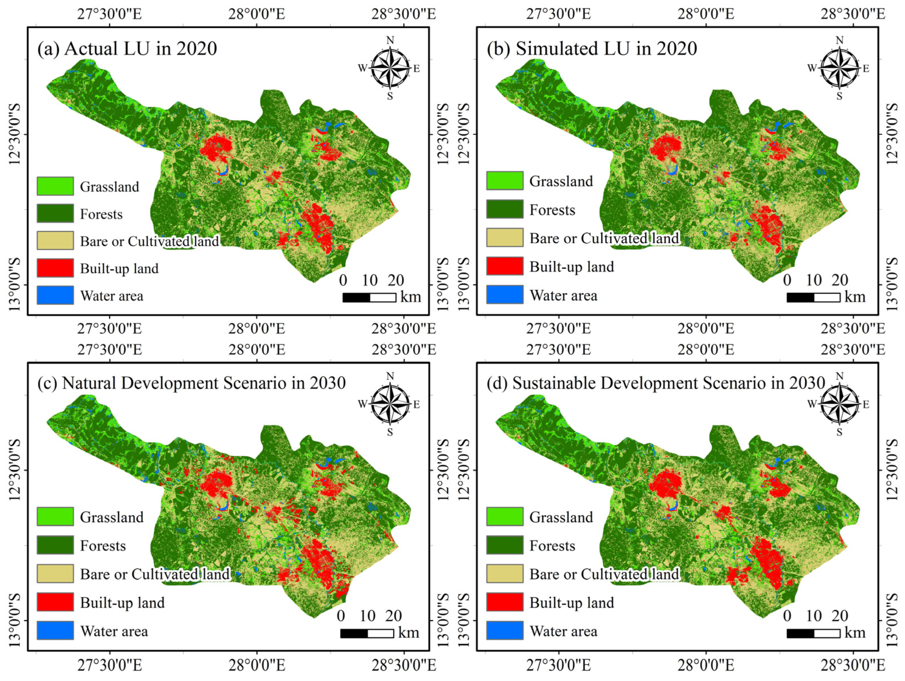
5.3. Analysis of Land-Use Simulation Results Under SDG Frame

This study analyzed land-use and population changes from 2000 to 2020 in the study area and applied the Spatial Cooperative Simulation (SCS) approach to model population distribution and land-use scenarios for 2030 for the CMFEZ and its neighboring cities under two scenarios: natural development and sustainable development. The results indicate that under the natural development scenario, without any policy interventions on land-use trends, unplanned development issues in the CMFEZ would escalate. It is projected that by 2030, 119.9 km² of land, currently of other types, will be converted into urban construction land, encroaching upon ecologically valuable land around urban areas. In the sustainable development scenario, considering urban habitation and surrounding ecological planning, unplanned expansion issues in the CMFEZ are mitigated while also preserving nearby forests and grasslands. Population growth would follow urban sustainable development trends, matching industrial development, leading to more people moving into Chambishi, the industrial hub, while the overcrowding issues in Kitwe are expected to be alleviated.

This study confirms that the data source of SDG 11.3.1 has been changed from previous administrative division-level statistics to high-resolution RS and geospatial data, which can strongly enhance the problem of rough and missing information at a fine scale [50]. The population increase rate of built-up areas in the CMFEZ and the neighboring cities is higher than the population increase rate in the same period, which in turn aggravates the problem of the rapid growth of the city and its population. The phenomenon of uncoordinated population and land growth is also very common in sub-Saharan African cities [51]. The conversion of a large portion of the former forests, grassland, and cultivated land to unplanned urban built-up areas due to low land acquisition prices and quick industrial development may be one explanation for this, which has increased the rate of land-use change.

5.4. Limitations and Future Perspectives

Monitoring the development of urban areas and the achievement of SDG 11 is influenced by a variety of factors. From a practical view, the geographic and regional policy frameworks of the sub-Saharan Africa (SSA) region have an impact on urban development; from a data view, there is a lack of early high-resolution remote sensing imagery and statistics in the region. Therefore, the uncertainty of future urban expansion and differences in urban development are the greatest limitations of this study. In order to more accurately monitor urban development in the SSA region, further research can be conducted to address the following issues.

Compared to the NTL image of large cities, the study area in this paper has relatively low luminance and the oversaturation of DMSP-OLS is not significant, which is the biggest uncertainty associated with the use of nightlight data. At the same time, the DMSP-OLS and VIIRS NTL images used in the study suffer from low spatial resolution and inaccuracies in measuring small-scale built-up urban areas. Therefore, it is quite challenging to accurately extract a long-term series of SSA urban development expansion.

In addition, in the simulation of urban land use and population, a multi-factor spatial cooperative CA simulation model is used, whose output raster has a lower spatial resolution, making it more difficult to reflect the intra-city planning changes from the perspective of blocks. In order to more deeply relate the results of the study to urban planning, future studies could consider simulating the functional evolution of vector plots in neighborhoods. [52] In order to fully investigate urban sprawl and monitor changes in SDG 11.3.1, efforts will be made to address these limitations and explore advanced modeling and data analysis methods.

More indicators need to be investigated in order to measure the sustainable development problems associated with urban expansion. High rates of urban and population expansion can lead to the overuse of land resources, environmental pollution, and social inequality, which are contrary to the goals of sustainable development. Future urban development in SSA requires more comprehensive policies and planning to achieve these goals. Our study is only a preliminary exploration, and more in-depth research is needed to understand the impacts of urbanization on sustainable development and the solutions to these challenges.

6. Conclusions

With the use of NTL data, remote sensing images, and geospatial data, this study thoroughly examines the dynamics of urban expansion, land use, and population change in Zambia’s surrounding cities and the Chambishi Multi-Facility Economic Zone (CMFEZ) from 2000 to 2020 in both the spatial and temporal dimensions. Guided by Sustainable Development Goal (SDG) 11, this study simulates land-use and population scenarios for the year 2030. Finally, based on the historical data as well as the simulated 2030 SDG 11 scenarios, the changes in the SDG 11.3.1 indicator, namely, urbanization trends and urban land consumption patterns, in the three decades from 2000 to 2030 were calculated in a spatialized form so as to provide recommendations for urban development planning within the research area. The main findings and key conclusions of the research are presented below:

It was found that the pseudo-invariant features (PIFs) method successfully extracted urban boundaries from nighttime lighting data with an average OA value of more than 86.7%, which effectively and accurately monitored urban sprawl and ensured the robustness of the data. CMFEZ and its neighboring cities generally show an expansion trend between 2000 and 2020, and although the rate of expansion is uneven across the cities, the overall direction of expansion is similar, which is consistent with the orientation of the industrial park. However, the lack of planned urbanization poses a challenge to achieving the SDG11 goals.

In addition, using the Spatial Cooperative Simulation (SCS) approach with initial simulation by the PLUS model, this study conducted a multi-scenario simulation of land-use population scenarios for 2030. The simulation results reveal that under the unplanned natural development scenario, the sprawl of urban built-up areas may intensify and the green space may reduce in the study area. The simulation results under the sustainable development scenario have the potential to achieve sustainable urban development as they are projected to adequately control the urban built-up area expansion and protect the peri-urban forests and grasslands, while the population still grows but at a slower rate and the spatial distribution of the population is further optimized.

From 2000 to 2020, the rate of urban expansion in the whole study area is lower than the population growth rate (LCRPGR < 1), and urban development is unbalanced. However, the average LCRPGR for the whole study region exhibits a notable rising tendency between 2020 and 2030, guided by the concept of sustainable development. The LCRPGR of most districts is also close to the ideal state (LCRPGR ≈ 1). The spatialized LCRPGR results highlight areas within the CMFEZ where interventions are needed to balance intra-urban sprawl with population growth.

The results of the study suggest that the integrated use of remote sensing for monitoring and planning urbanization processes is important for guiding sustainable urban development in Zambia and similar developing countries. Future research could further explore additional remote sensing data sources and advanced simulation models to improve the prediction accuracy and applicability of urban planning strategies.

References

1. Nations, U. Transforming Our World: The 2030 Agenda for Sustainable Development; United Nations, Department of Economic and Social Affairs: New York, NY, USA, 2015; Volume 1, p. 41. [Google Scholar]
2. UN-HABITAT. Metadata on SDG Indicator 11.3.1. Available online: https://unhabitat.org/sites/default/files/2022/08/sdg_indicator_metadata-11.3.1.pdf (accessed on 7 August 2024).
3. Akuraju, V.; Pradhan, P.; Haase, D.; Kropp, J.P.; Rybski, D. Relating SDG11 Indicators and Urban Scaling—An Exploratory Study. Sustain. Cities Soc. 2020, 52, 101853. [Google Scholar] [CrossRef]
4. Forget, Y.; Shimoni, M.; Gilbert, M.; Linard, C. Mapping 20 Years of Urban Expansion in 45 Urban Areas of Sub-Saharan Africa. Remote Sens. 2021, 13, 525. [Google Scholar] [CrossRef]
5. Xu, J.; Wang, X. Reversing Uncontrolled and Unprofitable Urban Expansion in Africa through Special Economic Zones: An Evaluation of Ethiopian and Zambian Cases. Sustainability 2020, 12, 9246. [Google Scholar] [CrossRef]
6. Chibbonta, W.; Mayondi, M.; Mulenga, R. A REFLECTION ON ZAMBIA’S DEVELOPMENT STRATEGIES SINCE INDEPENDENCE-1964 TO 2021. Available online: https://www.multiresearch.net/cms/publications/CFP26582022.pdf (accessed on 7 August 2024).
7. Mutale, I.; Franco, I.B.; Lamont, S. Zambia’s Mining Industry: A Closer Look at the Corporate Approaches to Sustainable Development of Konkola and Mopani Copper Mines. In Corporate Approaches to Sustainable Development; Franco, I.B., Ed.; Science for Sustainable Societies; Springer Nature: Singapore, 2022; pp. 73–88. ISBN 9789811664205. [Google Scholar]
8. Zhou, M.; Lu, L.; Guo, H.; Weng, Q.; Cao, S.; Zhang, S.; Li, Q. Urban Sprawl and Changes in Land-Use Efficiency in the Beijing–Tianjin–Hebei Region, China from 2000 to 2020: A Spatiotemporal Analysis Using Earth Observation Data. Remote Sens. 2021, 13, 2850. [Google Scholar] [CrossRef]
9. Wang, Y.; Huang, C.; Feng, Y.; Zhao, M.; Gu, J. Using Earth Observation for Monitoring SDG 11.3. 1-Ratio of Land Consumption Rate to Population Growth Rate in Mainland China. Remote Sens. 2020, 12, 357. [Google Scholar] [CrossRef]
10. Gao, K.; Yang, X.; Wang, Z.; Zhang, H.; Huang, C.; Zeng, X. Spatial Sustainable Development Assessment Using Fusing Multisource Data from the Perspective of Production-Living-Ecological Space Division: A Case of Greater Bay Area, China. Remote Sens. 2022, 14, 2772. [Google Scholar] [CrossRef]
11. Croft, T.A. Nighttime Images of the Earth from Space. Sci. Am. 1978, 239, 86–101. [Google Scholar] [CrossRef]
12. Milesi, C.; Elvidge, C.D.; Nemani, R.R.; Running, S.W. Assessing the Impact of Urban Land Development on Net Primary Productivity in the Southeastern United States. Remote Sens. Environ. 2003, 86, 401–410. [Google Scholar] [CrossRef]
13. Muthukrishnan, R.; Radha, M. Edge Detection Techniques for Image Segmentation. Int. J. Comput. Sci. Inf. Technol. 2011, 3, 259. [Google Scholar] [CrossRef]
14. Su, Y.; Chen, X.; Wang, C.; Zhang, H.; Liao, J.; Ye, Y.; Wang, C. A New Method for Extracting Built up Urban Areas Using DMSP-OLS Nighttime Stable Lights: A Case Study in the Pearl River Delta, Southern China. GIScience Remote Sens. 2015, 52, 218–238. [Google Scholar] [CrossRef]
15. Quarmby, N.A.; Cushnie, J.L. Monitoring Urban Land Cover Changes at the Urban Fringe from SPOT HRV Imagery in South-East England. Int. J. Remote Sens. 1989, 10, 953–963. [Google Scholar] [CrossRef]
16. Wu, K.; Wang, X. Aligning Pixel Values of DMSP and VIIRS Nighttime Light Images to Evaluate Urban Dynamics. Remote Sens. 2019, 11, 1463. [Google Scholar] [CrossRef]
17. Wei, Y.; Liu, H.; Song, W.; Yu, B.; Xiu, C. Normalization of Time Series DMSP-OLS Nighttime Light Images for Urban Growth Analysis with Pseudo Invariant Features. Landsc. Urban Plan. 2014, 128, 1–13. [Google Scholar] [CrossRef]
18. Li, S.; Liu, X.; Li, X.; Chen, Y. Simulation Model of Land Use Dynamics and Application: Progress and Prospects. J. Remote Sens. 2017, 21, 329–340. [Google Scholar] [CrossRef]
19. Liu, X.; Liang, X.; Li, X.; Xu, X.; Ou, J.; Chen, Y.; Li, S.; Wang, S.; Pei, F. A Future Land Use Simulation Model (FLUS) for Simulating Multiple Land Use Scenarios by Coupling Human and Natural Effects. Landsc. Urban Plan. 2017, 168, 94–116. [Google Scholar] [CrossRef]
20. Liang, X.; Guan, Q.; Clarke, K.C.; Liu, S.; Wang, B.; Yao, Y. Understanding the Drivers of Sustainable Land Expansion Using a Patch-Generating Land Use Simulation (PLUS) Model: A Case Study in Wuhan, China. Comput. Environ. Urban Syst. 2021, 85, 101569. [Google Scholar] [CrossRef]
21. Shang, S.; Du, S.; Du, S.; Zhu, S. Estimating Building-Scale Population Using Multi-Source Spatial Data. Cities 2021, 111, 103002. [Google Scholar] [CrossRef]
22. Yu, Y.; Yu, M.; Lin, L.; Chen, J.; Li, D.; Zhang, W.; Cao, K. National Green GDP Assessment and Prediction for China Based on a CA-Markov Land Use Simulation Model. Sustainability 2019, 11, 576. [Google Scholar] [CrossRef]
23. Guzman, L.A.; Camacho, R.; Herrera, A.R.; Beltrán, C. Modeling Population Density Guided by Land Use-Cover Change Model: A Case Study of Bogotá. Popul. Environ. 2022, 43, 553–575. [Google Scholar] [CrossRef]
24. Levin, N.; Kyba, C.C.; Zhang, Q.; de Miguel, A.S.; Román, M.O.; Li, X.; Portnov, B.A.; Molthan, A.L.; Jechow, A.; Miller, S.D. Remote Sensing of Night Lights: A Review and an Outlook for the Future. Remote Sens. Environ. 2020, 237, 111443. [Google Scholar] [CrossRef]
25. Baugh, K.; Elvidge, C.D.; Ghosh, T.; Ziskin, D. Development of a 2009 Stable Lights Product Using DMSP-OLS Data. Proc. Asia-Pac. Adv. Netw. 2010, 30, 114. [Google Scholar] [CrossRef]
26. Bian, J.; Li, A.; Lei, G.; Zhang, Z.; Nan, X.; Liang, L. Inter-Calibration of Nighttime Light Data between DMSP/OLS and NPP/VIIRS in the Economic Corridors of Belt and Road Initiative. In Proceedings of the IGARSS 2019—2019 IEEE International Geoscience and Remote Sensing Symposium, Yokohama, Japan, 28 July–2 August 2019; pp. 9028–9031. [Google Scholar]
27. Xie, Y.; Weng, Q. Updating Urban Extents with Nighttime Light Imagery by Using an Object-Based Thresholding Method. Remote Sens. Environ. 2016, 187, 1–13. [Google Scholar] [CrossRef]
28. Liu, L.; Liu, J.; Liu, Z.; Xu, X.; Wang, B. Analysis on the Spatio-Temporal Characteristics of Urban Expansion and the Complex Driving Mechanism: Taking the Pearl River Delta Urban Agglomeration as a Case. Complexity 2020, 2020, 8157143. [Google Scholar] [CrossRef]
29. Baojun, W.; Bin, S.; Inyang, H.I. GIS-Based Quantitative Analysis of Orientation Anisotropy of Contaminant Barrier Particles Using Standard Deviational Ellipse. Soil Sediment Contam. Int. J. 2008, 17, 437–447. [Google Scholar] [CrossRef]
30. Zhong Yang, Z.Y.; Lin AiWen, L.A.; Zhou ZhiGao, Z.Z. Evolution of the Pattern of Spatial Expansion of Urban Land Use in the Poyang Lake Ecological Economic Zone. Int. J. Environ. Res. Public Health 2019, 16, 117. [Google Scholar] [CrossRef]
31. Tu, W.; Gao, W.; Li, M.; Yao, Y.; He, B.; Huang, Z.; Zhang, J.; Guo, R. Spatial Cooperative Simulation of Land Use-Population-Economy in the Greater Bay Area, China. Int. J. Geogr. Inf. Sci. 2024, 38, 381–406. [Google Scholar] [CrossRef]
32. Huang, C.; Zhou, Y.; Wu, T.; Zhang, M.; Qiu, Y. A Cellular Automata Model Coupled with Partitioning CNN-LSTM and PLUS Models for Urban Land Change Simulation. J. Environ. Manag. 2024, 351, 119828. [Google Scholar] [CrossRef] [PubMed]
33. Wang, J.; Bretz, M.; Dewan, M.A.A.; Delavar, M.A. Machine Learning in Modelling Land-Use and Land Cover-Change (LULCC): Current Status, Challenges and Prospects. Sci. Total Environ. 2022, 822, 153559. [Google Scholar] [CrossRef]
34. Gao, L.; Tao, F.; Liu, R.; Wang, Z.; Leng, H.; Zhou, T. Multi-Scenario Simulation and Ecological Risk Analysis of Land Use Based on the PLUS Model: A Case Study of Nanjing. Sustain. Cities Soc. 2022, 85, 104055. [Google Scholar] [CrossRef]
35. Jenks, G.F. The Data Model Concept in Statistical Mapping. Int. Yearb. Cartogr. 1967, 7, 186–190. [Google Scholar]
36. Pontius, R.G. Quantification Error versus Location Error in Comparison of Categorical Maps (Vol 66, Pg 1011, 2000). Photogramm. Eng. Remote Sens. 2001, 67, 540. [Google Scholar]
37. Pontius, R.G.; Boersma, W.; Castella, J.-C.; Clarke, K.; De Nijs, T.; Dietzel, C.; Duan, Z.; Fotsing, E.; Goldstein, N.; Kok, K.; et al. Comparing the Input, Output, and Validation Maps for Several Models of Land Change. Ann. Reg. Sci. 2008, 42, 11–37. [Google Scholar] [CrossRef]
38. Chai, T.; Draxler, R.R. Root Mean Square Error (RMSE) or Mean Absolute Error (MAE). Geosci. Model Dev. Discuss. 2014, 7, 1525–1534. [Google Scholar]
39. Li, C.; Cai, G.; Sun, Z. Urban Land-Use Efficiency Analysis by Integrating LCRPGR and Additional Indicators. Sustainability 2021, 13, 13518. [Google Scholar] [CrossRef]
40. Deng, Y.; Qi, W.; Fu, B.; Wang, K. Geographical Transformations of Urban Sprawl: Exploring the Spatial Heterogeneity across Cities in China 1992–2015. Cities 2020, 105, 102415. [Google Scholar] [CrossRef]
41. Sirko, W.; Kashubin, S.; Ritter, M.; Annkah, A.; Bouchareb, Y.S.E.; Dauphin, Y.; Keysers, D.; Neumann, M.; Cisse, M.; Quinn, J. Continental-Scale Building Detection from High Resolution Satellite Imagery. arXiv 2021, arXiv:2107.12283. [Google Scholar]
42. Plc, K.I.L. ZCCM Investments Holdings Zambia—Copperbelt Environment Project: Environmental Impact Assessment. Available online: https://documents.worldbank.org/en/publication/documents-reports/documentdetail/152831468766181491/Zambia-Copperbelt-Environment-Project-environmental-impact-assessment (accessed on 7 July 2024).
43. Huang, M.; Zhang, X. Construction of the Zambia–China Economic and Trade Cooperation Zone and South–South Cooperation. In South-South Cooperation and Chinese Foreign Aid; Huang, M., Xu, X., Mao, X., Eds.; Springer: Singapore, 2019; pp. 257–273. ISBN 9789811320019. [Google Scholar]
44. Kapobe, J.; Mazala, C.; Phiri, R. Kitwe Black Mountain-Is Zambia Realising the True Value from It? J. Nat. Appl. Sci. 2019, 3, 62–72. [Google Scholar] [CrossRef]
45. Okeyinka, Y. Housing in the Third World Cities and Sustainable Urban Developments. Dev. Ctry. Stud. 2014, 4, 112–120. [Google Scholar]
46. Simwanda, M.; Murayama, Y.; Ranagalage, M. Modeling the Drivers of Urban Land Use Changes in Lusaka, Zambia Using Multi-Criteria Evaluation: An Analytic Network Process Approach. Land Use Policy 2020, 92, 104441. [Google Scholar] [CrossRef]
47. Central Statistical Office Zambia. 2000 Census of Population and Housing. Available online: https://www.zamstats.gov.zm/wp-content/uploads/2023/12/2000-Census-of-population-and-housing-summary-report.pdf (accessed on 7 August 2024).
48. Central Statistical Office Zambia. 2010 Census of Population and Housing. Available online: https://www.zamstats.gov.zm/wp-content/uploads/2023/12/National-Analytical-Report-2010-Census.pdf (accessed on 7 August 2024).
49. Isbell, T.; Dryding, D. Zambians See Progress on Education Despite Persistent Inequalities. 2019. Available online: https://www.afrobarometer.org/wp-content/uploads/2022/02/ab_r7_dispatchno272_zambians_see_progress_on_education.pdf (accessed on 7 August 2024).
50. Liu, S.; Yan, Y.; Hu, B. Satellite Monitoring of the Urban Expansion in the Pearl River–Xijiang Economic Belt and the Progress towards SDG11.3.1. Remote Sens. 2023, 15, 5209. [Google Scholar] [CrossRef]
51. Mudau, N.; Mwaniki, D.; Tsoeleng, L.; Mashalane, M.; Beguy, D.; Ndugwa, R. Assessment of SDG Indicator 11.3. 1 and Urban Growth Trends of Major and Small Cities in South Africa. Sustainability 2020, 12, 7063. [Google Scholar] [CrossRef]
52. Guan, Q.; Li, J.; Zhai, Y.; Liang, X.; Yao, Y. HashGAT-VCA: A Vector Cellular Automata Model with Hash Function and Graph Attention Network for Urban Land-Use Change Simulation. Landsc. Urban Plan 2024, 250, 105145. [Google Scholar] [CrossRef]
Figure 1. (a) Map of Research Area. (b) Location of Research Area in Zambia. (c) Remote Sensing Image of Industrial Parks in MFEZ.
Remotesensing 16 02995 g001
Figure 2. Workflow of the study.
Remotesensing 16 02995 g002
Figure 3. Driving factors for land-use population cooperative simulation.
Remotesensing 16 02995 g003
Figure 4. Extracted Urban Boundaries for 2000, 2005, and 2010 using the PIFs Method: (ac) and STS Method: (df).
Remotesensing 16 02995 g004
Figure 5. Change in Urban Built-up Areas from 2000 to 2020.
Remotesensing 16 02995 g005
Figure 6. (a) Built-up Area Statistics By Year. (b) Growth Rate of Built-up Area Per 5 Years.
Remotesensing 16 02995 g006
Figure 7. Changes in the direction and trajectory of migration in the CMFEZ and surrounding districts urban built-up area, 2000–2020.
Remotesensing 16 02995 g007
Figure 8. LULC Transfer Chord Chart in (a) 2000–2010; (b)2010–2020.
Remotesensing 16 02995 g008
Figure 9. Spatial Distribution of LULC and Population in Research Area in (a,d) 2000; (b,e) 2010; (c,f) 2020.
Remotesensing 16 02995 g009
Figure 10. (a) Actual LU in 2020; (b) Simulated LU in 2020; (c) Natural Development Scenario in 2030; (d) Sustainable Development Scenario in 2030.
Remotesensing 16 02995 g010
Figure 11. (a) Population distribution in 2020; (b) simulated population distribution in 2030; (c) population difference in 2020–2030.
Remotesensing 16 02995 g011
Figure 12. Temporal Variation in LCR and PGR in all districts.
Remotesensing 16 02995 g012
Figure 13. (ac) Spatial distribution of LCRPGR in three time periods; (d) Temporal changes in LCRPGR in the study area over the period 2000–2030.
Remotesensing 16 02995 g013
Figure 14. (a) Development Potential of the Built-up area; (b) Contribution to the growth of the built-up area.
Remotesensing 16 02995 g014