
Cartographic Generalization of Islands Using Remote Sensing Images for Multiscale Representation


Abstract
1. Introduction
2. Related Works
2.1. Aggregation
2.2. Simplification
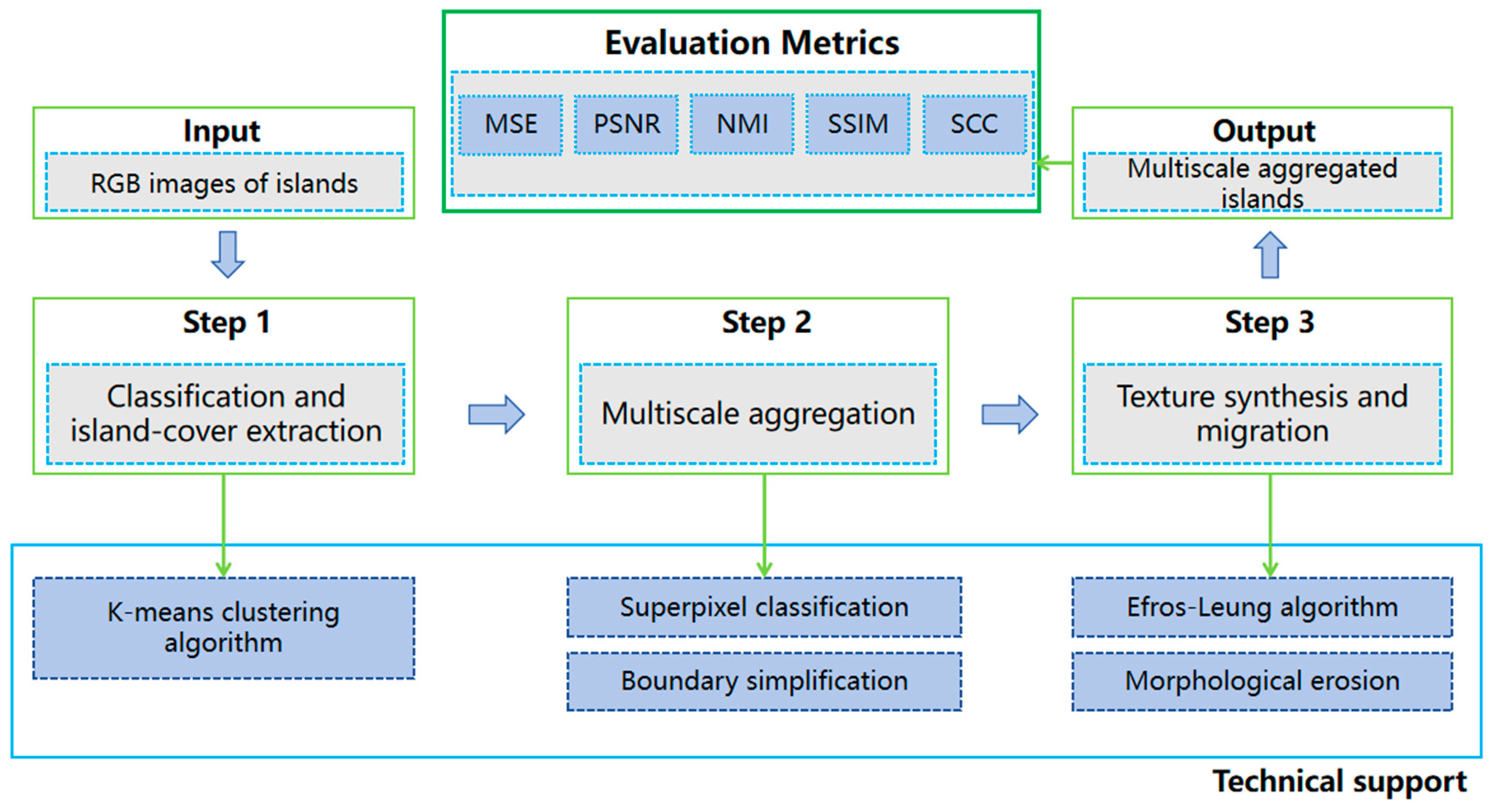
3. Methods
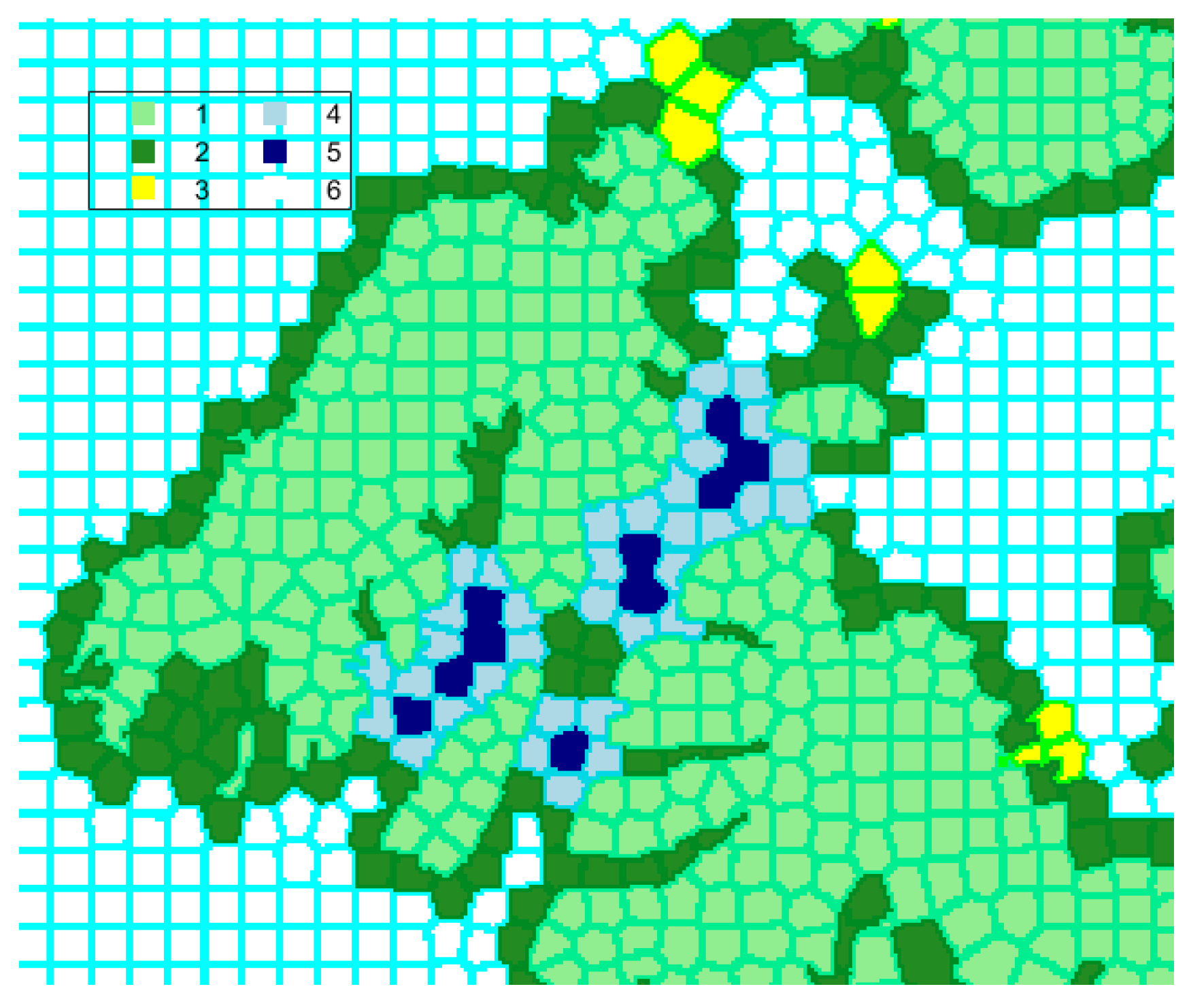
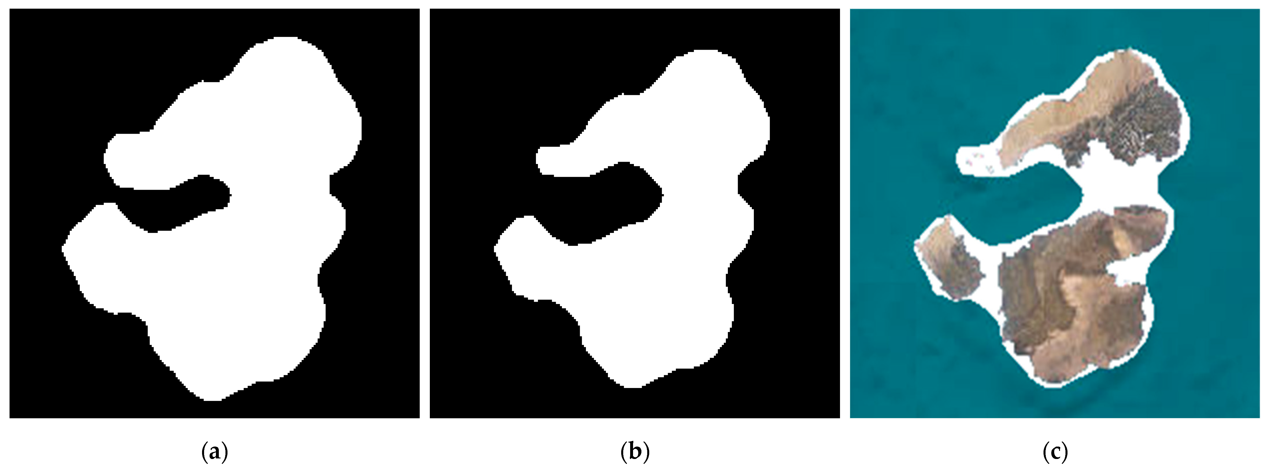
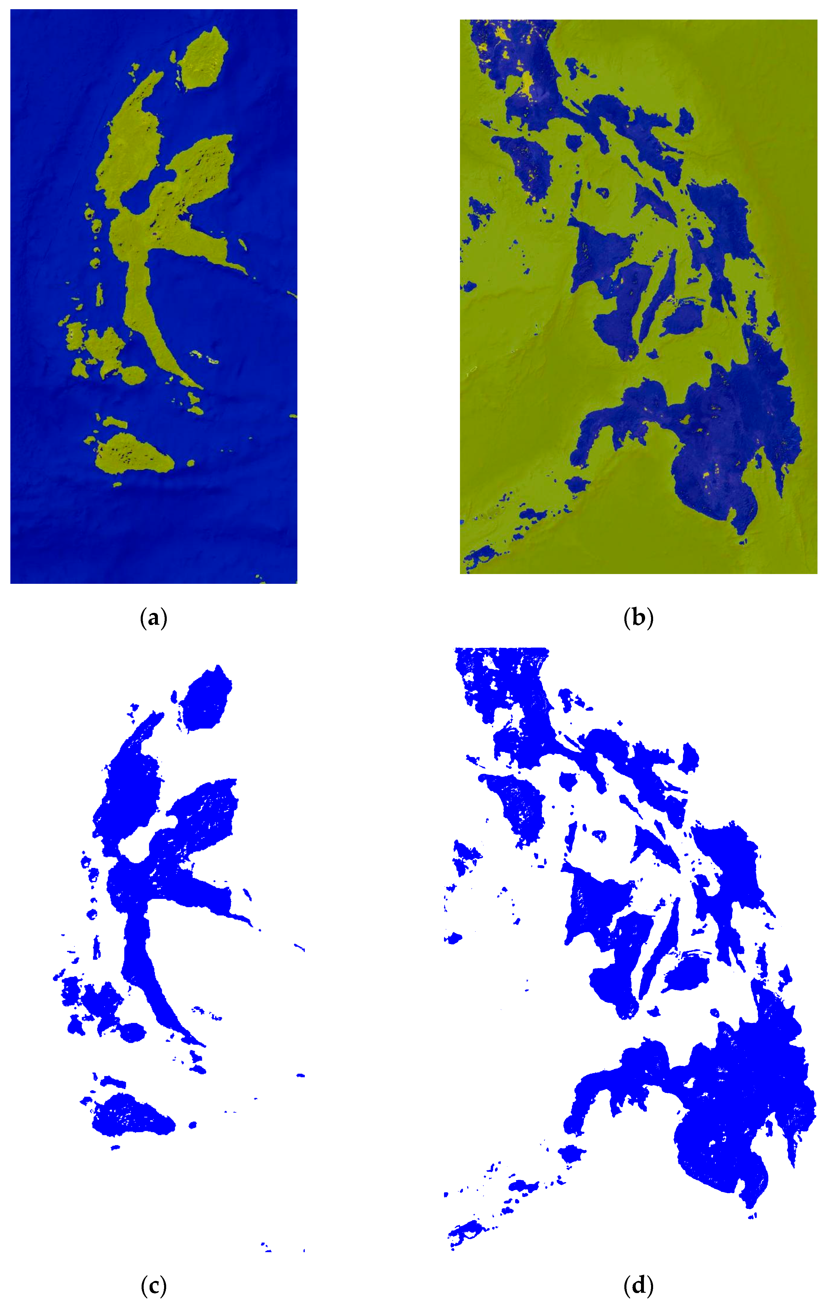
3.1. Island-Cover Extraction
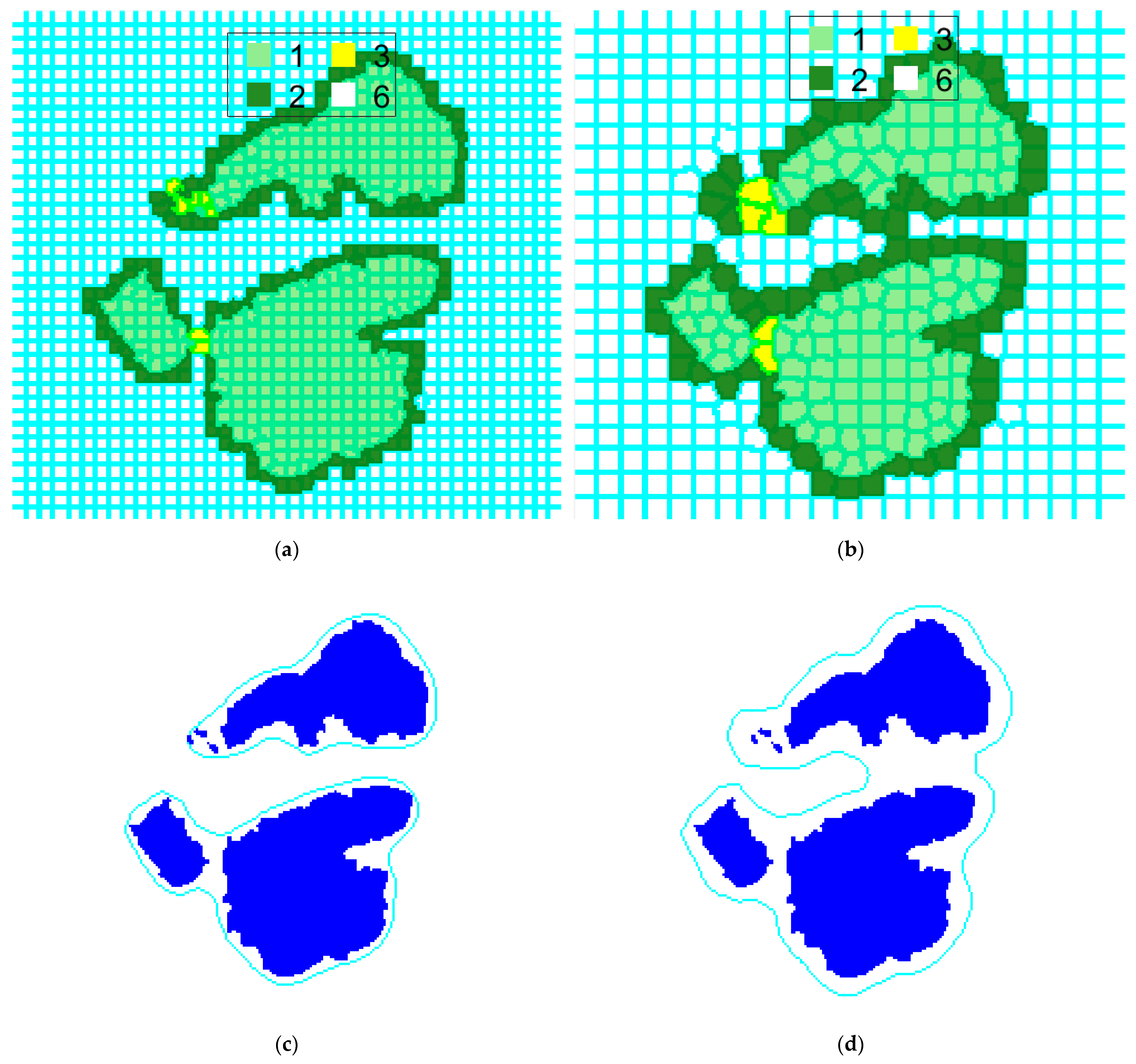
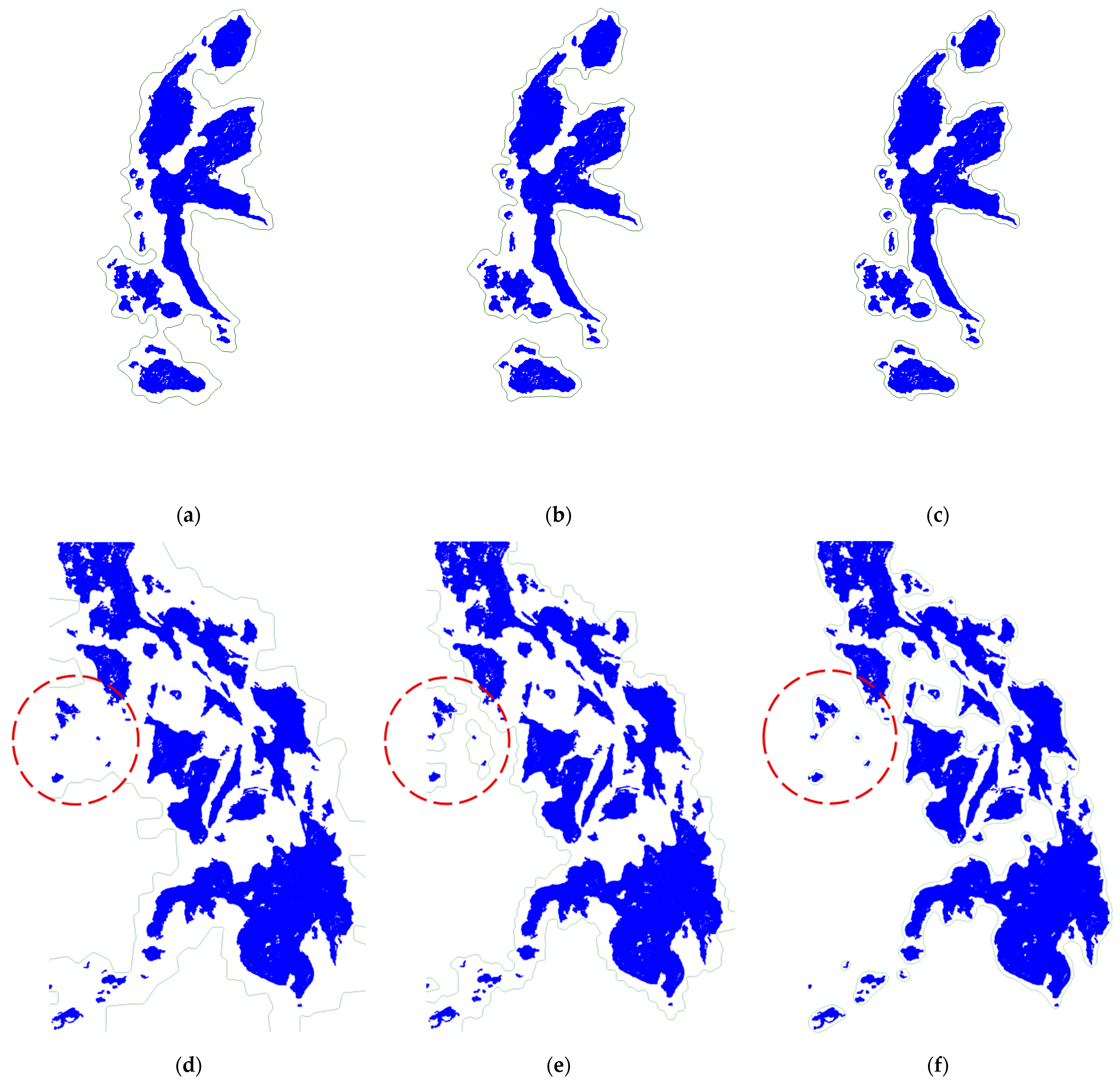
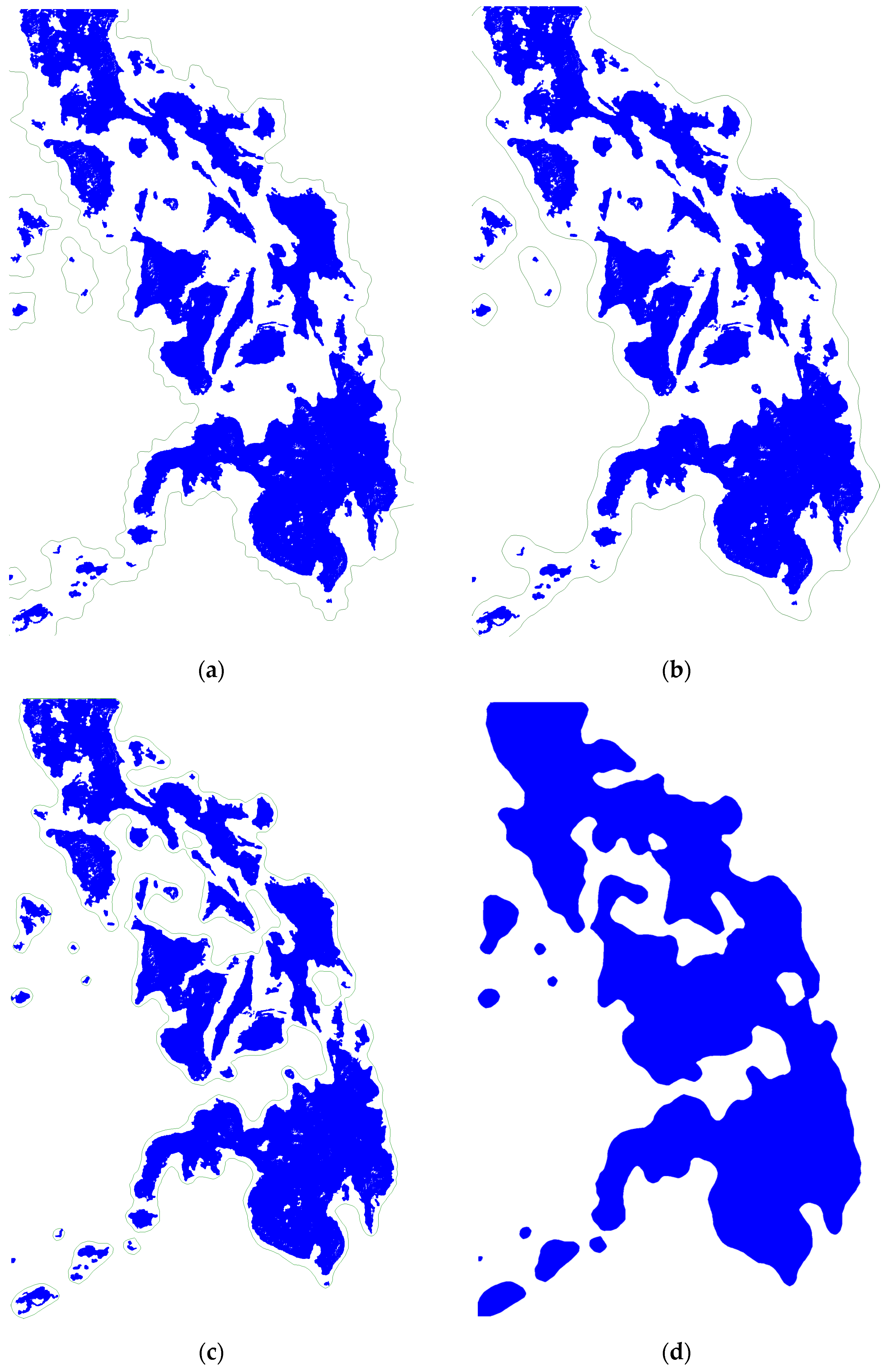
3.2. Islands Aggregation
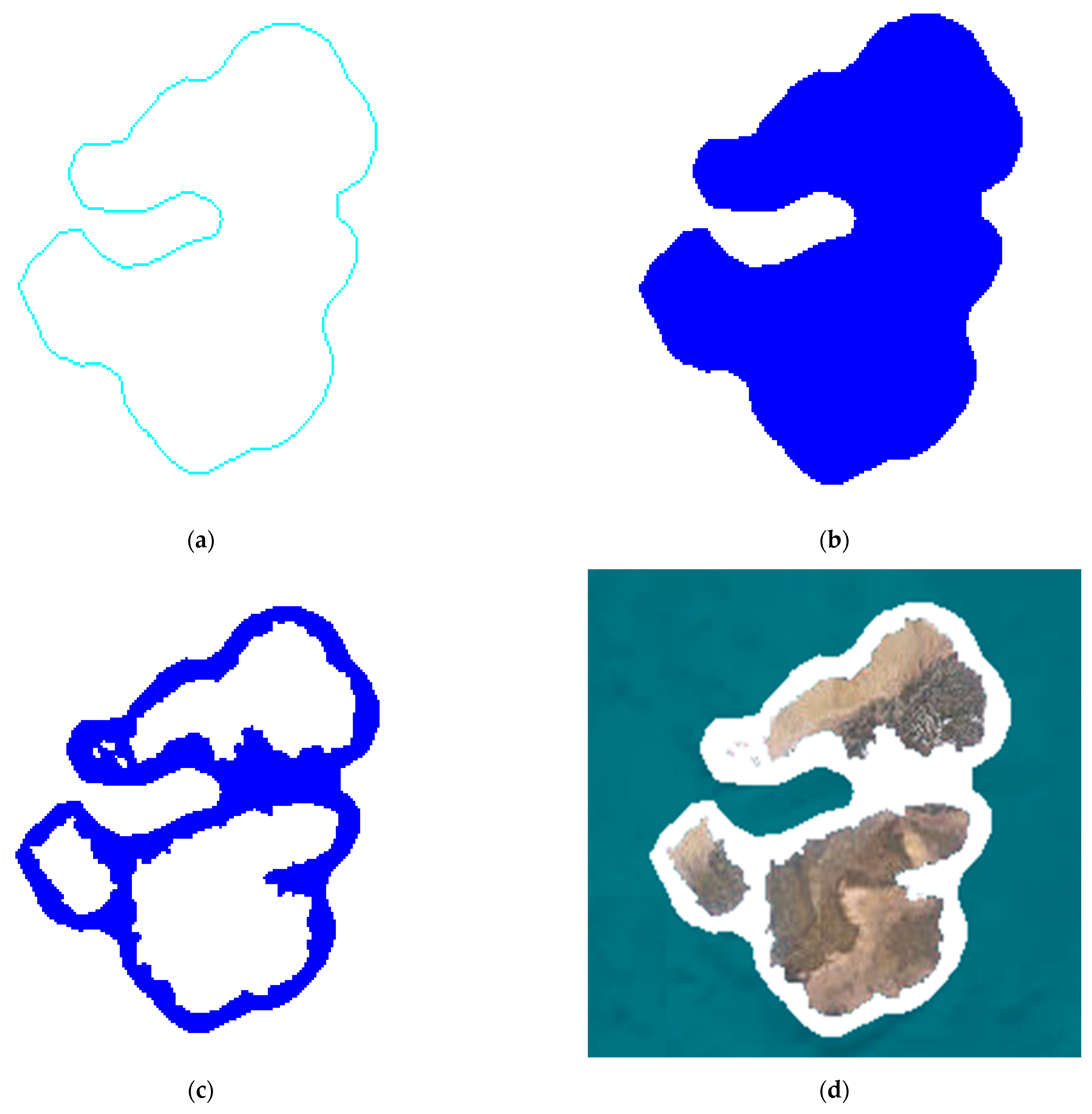
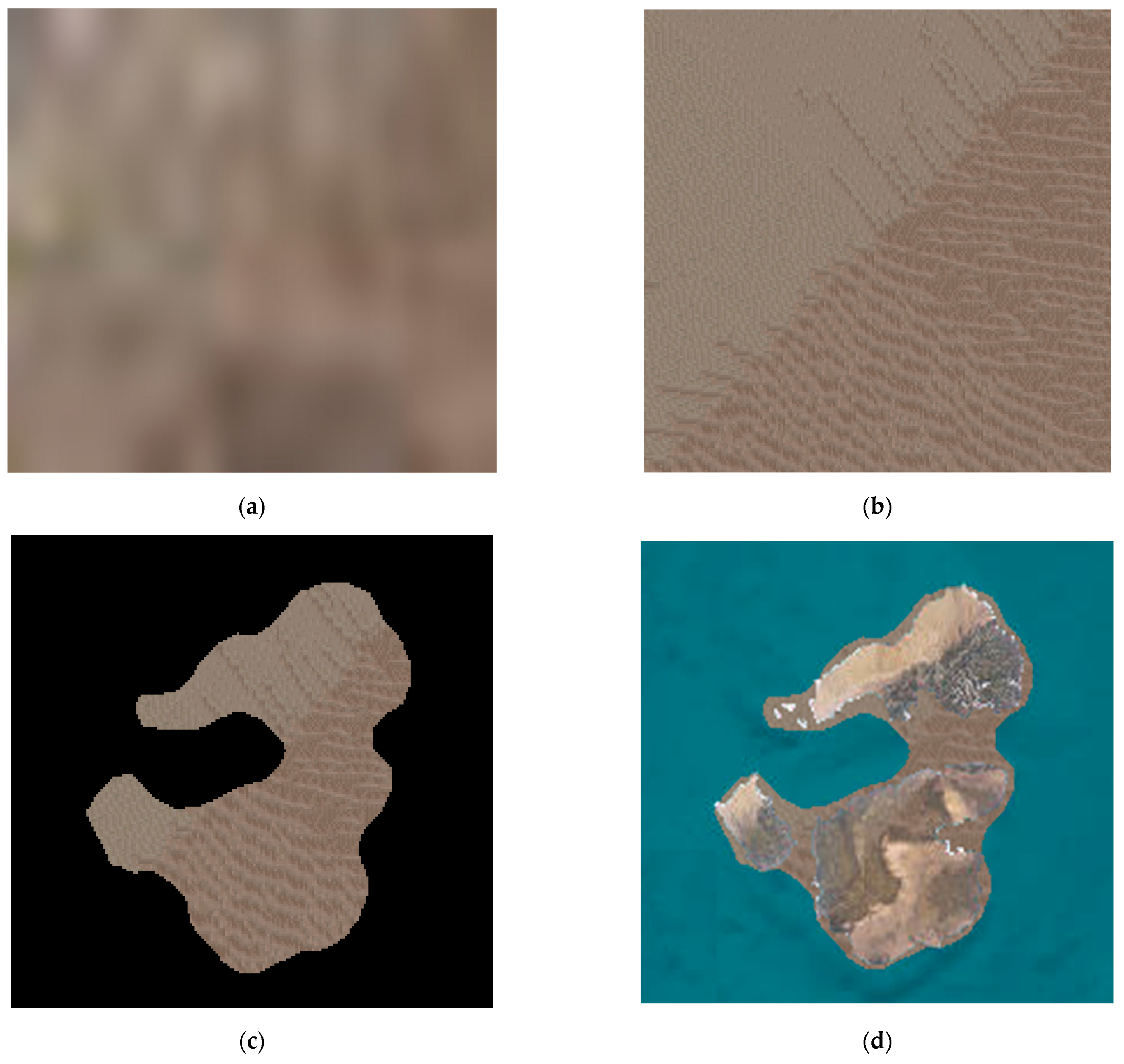
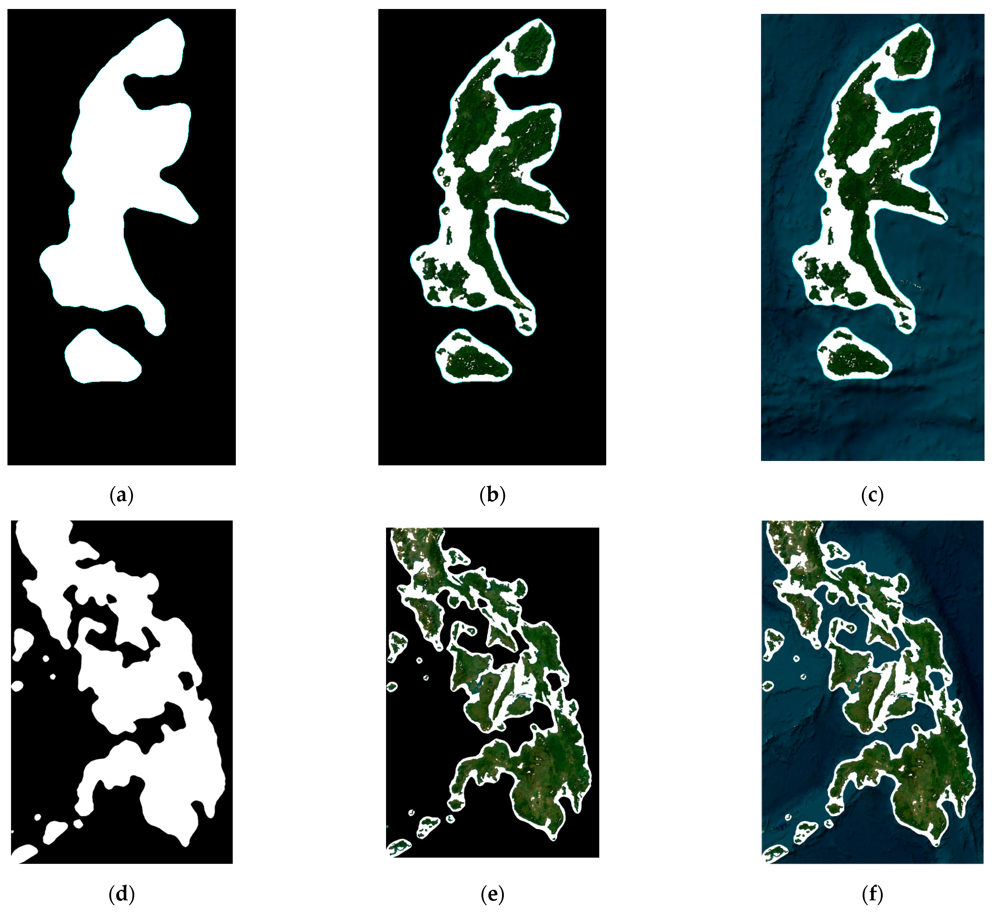
3.3. Texture Migration
4. Experiments
4.1. Dataset
4.2. Experimental Procedure
4.3. Experimental Results and Evaluation of Metrics
5. Summary
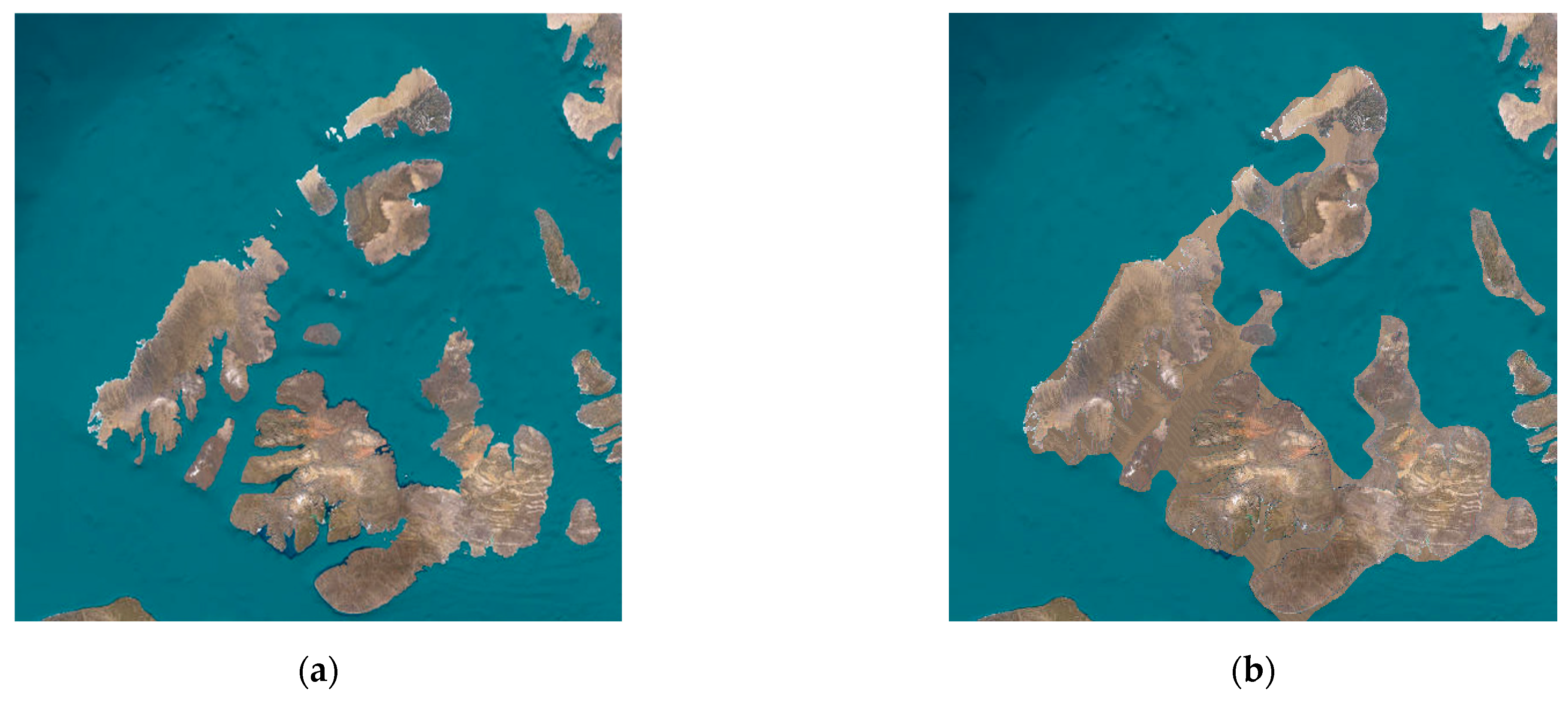
- Traditional vector-based methods often lose original textures when aggregating planar features, and raster-based aggregation methods cannot eliminate gaps between islands. However, our proposed method can preserve the original textures while filling the gaps between islands during the aggregating process.
- In contrast to traditional aggregating techniques, our method achieves smoother boundaries and sharper textures, thereby enhancing visualization quality;
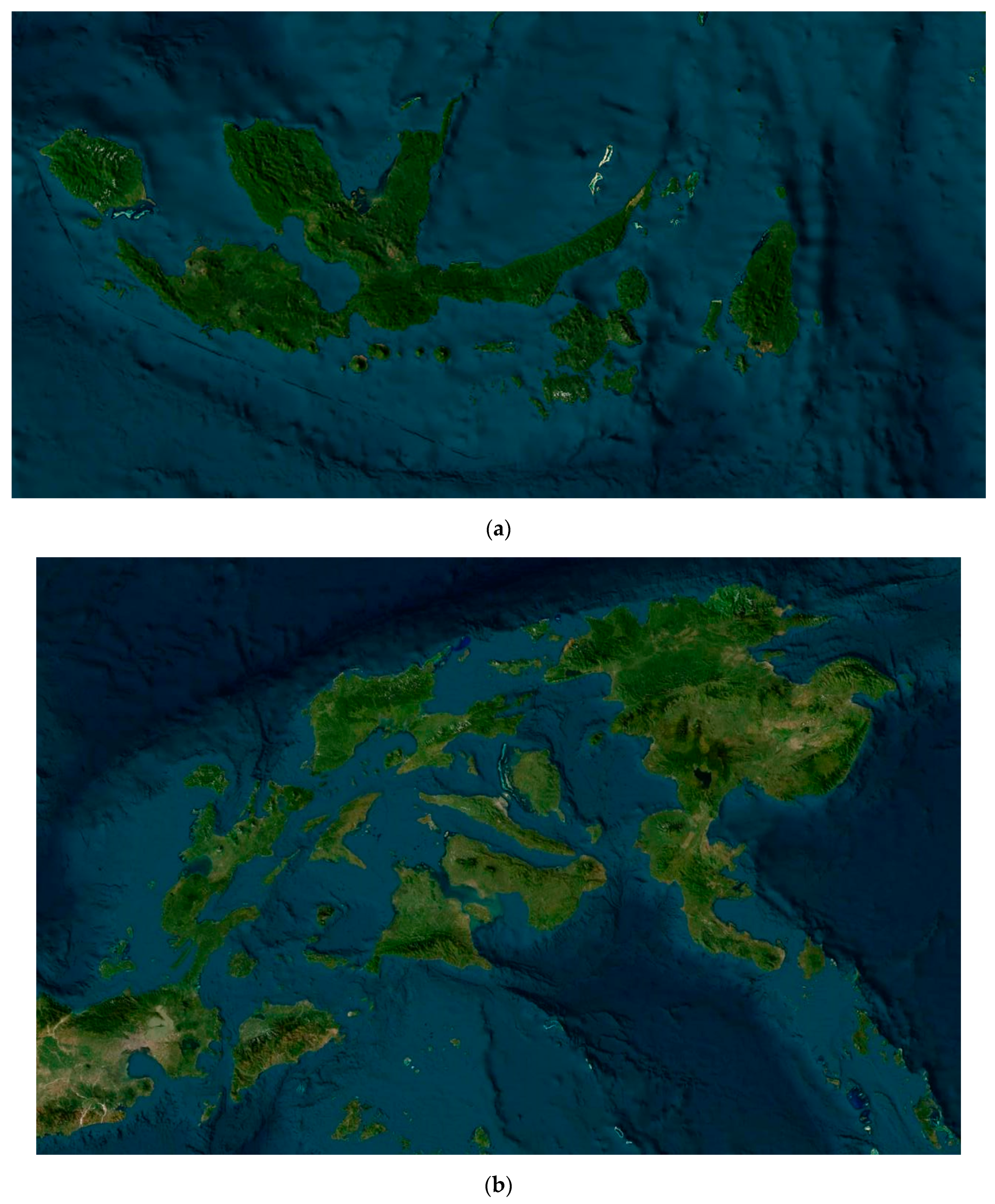
- Unlike traditional methods limited to a single scale, our approach allows for the generation of aggregated results at varying scales tailored to specific requirements.
Author Contributions
Funding
Data Availability Statement
Conflicts of Interest
References
- Dollár, P.; Appel, R.; Belongie, S.; Perona, P. Fast Feature Pyramids for Object Detection. IEEE Trans. Pattern Anal. Mach. Intell. 2014, 36, 1532–1545. [Google Scholar] [CrossRef] [PubMed]
- Simoncelli, E.P.; Freeman, W.T. The steerable pyramid: A flexible architecture for multi-scale derivative computation. Proc. Int. Conf. Image Process. 1995, 3, 444–447. [Google Scholar]
- Freeman, W.T.; Adelson, E.H. The design and use of steerable filters. IEEE Trans. Pattern Anal. Mach. Intell. 1991, 13, 891–906. [Google Scholar] [CrossRef]
- Buades, A.; Coll, B.; Morel, J.M. A non-local algorithm for image denoising. Proc. IEEE Comput. Soc. Conf. Comput. Vis. Pattern Recognit. 2005, 2, 60–65. [Google Scholar]
- Liu, L.; Li, W.; Qiu, H. Research on Principles and Methods of Sparse Island Cartographic Generalization. Sci. Surv. Mapp. 2013, 38, 117–119. [Google Scholar] [CrossRef]
- Beard, M.K. Knowledge-based generalization of geologic maps. Comput. Geosci. 1991, 17, 1073–1083. [Google Scholar]
- Ruas, A.; Lagrange, J.P. Data and knowledge modeling for generalization. In GIS and Generalization: Methodology and Practice; Muller, J.C., Lagrange, J.P., Weibel, R., Eds.; Taylor & Francis: London, UK, 1995; pp. 73–90. [Google Scholar]
- Wertheimer, M. Laws of Organization in Perceptual Forms. In A Source Book of Gestalt Psychology; Ellis, W.D., Ed.; Harcourt, Brace: New York, NY, USA, 1938; pp. 71–88. [Google Scholar]
- Li, C.; Yin, Y.; Wu, P.; Wu, W. An area merging method in map generalization considering typical characteristics of structured geographic objects. Cartogr. Geogr. Inf. Sci. 2021, 48, 210–224. [Google Scholar] [CrossRef]
- Ai, T.; Zhang, X. The aggregation of urban building clusters based on the skeleton partitioning of gap space. In The European Information Society; Springer: Berlin/Heidelberg, Germany, 2007; pp. 153–170. [Google Scholar]
- Guo, P.; Li, C.; Yin, Y. Classification and filtering of constrained Delaunay triangulation for automated building aggregation. ISPRS J. Photogramm. Remote Sens. 2021, 176, 282–294. [Google Scholar]
- Zhang, F.; Sun, Q.; Ma, J.; Lyu, Z.; Huang, Z. A polygonal buildings aggregation method considering obstacle elements and visual clarity. Geocarto Int. 2023, 38, 2266672. [Google Scholar] [CrossRef]
- Guo, R.; Ai, T. Simplification and aggregation of building polygon in automatic map generalization. J. Wuhan Tech. Univ. Surv. Mapp. 2000, 25, 25–30. [Google Scholar]
- He, X.; Zhang, X.; Yang, J. Progressive amalgamation of building clusters for map generalization based on scaling subgroups. ISPRS Int. J. Geo-Inf. 2018, 7, 116. [Google Scholar] [CrossRef]
- Li, C.; Yin, Y.; Liu, X.; Wu, P. An automated processing method for agglomeration areas. ISPRS Int. J. Geo-Inf. 2018, 7, 204. [Google Scholar] [CrossRef]
- Feng, Y.; Thiemann, F.; Sester, M. Learning Cartographic Building Generalization with Deep Convolutional Neural Networks. ISPRS Int. J. Geo-Inf. 2019, 8, 258. [Google Scholar] [CrossRef]
- Douglas, D.H.; Peucker, T.K. Algorithms for the reduction of the number of points required to represent a digitized line or its caricature. Cartogr. Int. J. Geogr. Inf. Geovisualization 1973, 10, 112–122. [Google Scholar] [CrossRef]
- Ai, T.; Zhou, Q.; Zhang, X.; Huang, Y.; Zhou, M. A simplification of ria coastline with geomorphologic characteristics preserved. Mar. Geod. 2014, 37, 167–186. [Google Scholar] [CrossRef]
- Ai, T.; Ke, S.; Yang, M.; Li, J. Envelope generation and simplification of polylines using Delaunay triangulation. Int. J. Geogr. Inf. Sci. 2017, 31, 297–319. [Google Scholar] [CrossRef]
- Visvalingam, M.; Whyatt, J.D. Line generalisation by repeated elimination of points. Cartogr. J. 1993, 30, 46–51. [Google Scholar] [CrossRef]
- Zhang, J.; Yuan, C.; Tong, X. A least-squares-adjustment-based method for automated map generalization of settlement areas in GIS. In Proceedings of the Geoinformatics 2006: Geospatial Information Science, Wuhan, China, 28–30 October 2006; SPIE: Bellingham, WA, USA, 2006; Volume 6420, p. 64200K. [Google Scholar]
- Chen, W.; Long, Y.; Shen, J.; Li, W. Structure Recognition and Progressive Simplification of the Concaves of Building Polygon Based on Constrained D-TIN. Geomat. Inf. Sci. Wuhan Univ. 2011, 36, 584–587. [Google Scholar]
- Meijers, M. Building simplification using offset curves obtained from the straight skeleton. In Proceedings of the 19th ICA Workshop on Generalisation and Multiple Representation, Helsinki, Finland, 14 June 2016. [Google Scholar]
- Kada, M. Aggregation of 3D buildings using a hybrid data approach. Cartogr. Geogr. Inf. Sci. 2011, 38, 153–160. [Google Scholar] [CrossRef]
- Cheng, B.; Liu, Q.; Li, X.; Wang, Y. Building simplification using backpropagation neural networks: A combination of cartographers’ expertise and raster-based local perception. GIScience Remote Sens. 2013, 50, 527–542. [Google Scholar] [CrossRef]
- Yang, M.; Yuan, T.; Yan, X.; Ai, T.; Jiang, C. A hybrid approach to building simplification with an evaluator from a backpropagation neural network. Int. J. Geogr. Inf. Sci. 2022, 36, 280–309. [Google Scholar] [CrossRef]
- Stillwell, J.; Daras, K.; Bell, M. Spatial Aggregation Methods for Investigating the MAUP Effects in Migration Analysis. Appl. Spat. Anal. 2018, 11, 693–711. [Google Scholar] [CrossRef]
- Efros, A.A.; Leung, T.K. Texture Synthesis by Non-parametric Sampling. In Proceedings of the IEEE International Conference on Computer Vision (ICCV’99), Corfu, Greece, 20–25 September 1999; pp. 1033–1038. [Google Scholar] [CrossRef]
- MacQueen, J.B. Some methods for classification and analysis of multivariate observations. In Proceedings of the Fifth Berkeley Symposium on Mathematical Statistics and Probability, Berkeley, CA, USA, 21 June–18 July 1965; Volume 1: Statistics. Le Cam, L.M., Neyman, J., Eds.; University of California Press: Berkeley, CA, USA, 1967; pp. 281–297. [Google Scholar]
- Wang, P.; Zeng, G.; Gan, R.; Wang, J.; Zha, H. Superpixel Segmentation Based on Multiple Seed Growth. In Proceedings of the 2017 International Symposium on Intelligent Signal Processing and Communication Systems (ISPACS), Xiamen, China, 6–9 November 2017; pp. 1–6. [Google Scholar]
- Shen, Y.; Ai, T.; Li, W.; Yang, M.; Feng, Y. A polygon aggregation method with global feature preservation using superpixel segmentation. Comput. Environ. Urban Syst. 2019, 75, 117–131. [Google Scholar] [CrossRef]
- Auer, M.; Zipf, A. 3D WebGIS: From Visualization to Analysis. An Efficient Browser-Based 3D Line-of-Sight Analysis. ISPRS Int. J. Geo-Inf. 2018, 7, 279. [Google Scholar] [CrossRef]
- Gavaskar, R.G.; Chaudhury, K.N. Fast Adaptive Bilateral Filtering. Trans. Image Process. 2019, 28, 779–790. [Google Scholar] [CrossRef]
- Zhang, K.; Zuo, W.; Chen, Y.; Meng, D.; Zhang, L. Beyond a Gaussian Denoiser: Residual Learning of Deep CNN for Image Denoising. IEEE Trans. Image Process. 2017, 26, 3142–3155. [Google Scholar] [CrossRef]
- Wachowiak, M.P.; Smoliková, R.; Tourassi, G.D.; Elmaghraby, A.S. Similarity Metrics Based on Nonadditive Entropies for 2D–3D Multimodal Biomedical Image Registration. In Medical Imaging 2003: Image Processing; Sonka, M., Fitzpatrick, J.M., Eds.; SPIE: Bellingham, WA, USA, 2003; Volume 5032, pp. 1090–1100. [Google Scholar]


| Sulawesi Island | MSE | PSNR | NMI | SSIM | SCC | Area (Pixels) |
|---|---|---|---|---|---|---|
| Original | 0 | inf | 1 | 1 | 1 | 72,716 |
| Mean Filtering | 4.062966665 | 42.04 | 0.5853 | 0.970603887 | 0.9479 | |
| Median Filtering | 3.374132156 | 42.85 | 0.6555 | 0.97418511 | 0.9501 | |
| Fast Adaptive Bilateral Filtering | 11.610228856404623 | 37.48 | 0.4258 | 0.9068859377076354 | 0.9576 | |
| CNN + Gaussian Blur | 19.700342814127605 | 35.19 | 0.2786 | 0.8411278436573086 | 0.8788 | |
| N = 2500, len = 17 | 8.240512848 | 38.97 | 0.837 | 0.921223914 | 0.8612 | 122,520 |
| N = 1800, len = 40 | 10.82569504 | 37.79 | 0.7951 | 0.905779965 | 0.8605 | 136,301 |
| N = 7000, len = 30 | 6.943405151 | 39.72 | 0.8582 | 0.926534499 | 0.8639 | 114,136 |
| Philippine Archipelago | MSE | PSNR | NMI | SSIM | SCC | Area (Pixels) |
|---|---|---|---|---|---|---|
| Original | 0 | inf | 1 | 1 | 1 | 657,615 |
| Mean Filtering | 8.830849365 | 38.67 | 0.5484 | 0.945734931 | 0.9440 | |
| Median Filtering | 7.667456009 | 39.28 | 0.6013 | 0.949695802 | 0.9487 | |
| Fast Adaptive Bilateral Filtering | 17.1392986398493 | 35.79 | 0.4097 | 0.867839697459523 | 0.9533 | |
| CNN + Gaussian Blur | 25.9185290249534 | 33.99 | 0.3245 | 0.7777573460086513 | 0.8912 | |
| N = 1800, len = 65 | 32.76713031 | 32.98 | 0.4788 | 0.794131297 | 0.8953 | 1,441,493 |
| N = 6400, len = 75 | 24.0629642 | 34.32 | 0.5361 | 0.841412155 | 0.9062 | 1,224,822 |
| N = 9000, len = 50 | 16.88695558 | 35.86 | 0.581 | 0.872360166 | 0.9231 | 1,055,782 |
Disclaimer/Publisher’s Note: The statements, opinions and data contained in all publications are solely those of the individual author(s) and contributor(s) and not of MDPI and/or the editor(s). MDPI and/or the editor(s) disclaim responsibility for any injury to people or property resulting from any ideas, methods, instructions or products referred to in the content. |
© 2024 by the authors. Licensee MDPI, Basel, Switzerland. This article is an open access article distributed under the terms and conditions of the Creative Commons Attribution (CC BY) license (https://creativecommons.org/licenses/by/4.0/).
Share and Cite
Li, R.; Shen, Y.; Dai, W. Cartographic Generalization of Islands Using Remote Sensing Images for Multiscale Representation. Remote Sens. 2024, 16, 2971. https://doi.org/10.3390/rs16162971
Li R, Shen Y, Dai W. Cartographic Generalization of Islands Using Remote Sensing Images for Multiscale Representation. Remote Sensing. 2024; 16(16):2971. https://doi.org/10.3390/rs16162971
Chicago/Turabian StyleLi, Renzhu, Yilang Shen, and Wanyue Dai. 2024. "Cartographic Generalization of Islands Using Remote Sensing Images for Multiscale Representation" Remote Sensing 16, no. 16: 2971. https://doi.org/10.3390/rs16162971
APA StyleLi, R., Shen, Y., & Dai, W. (2024). Cartographic Generalization of Islands Using Remote Sensing Images for Multiscale Representation. Remote Sensing, 16(16), 2971. https://doi.org/10.3390/rs16162971