Pose Estimation Based on Bidirectional Visual–Inertial Odometry with 3D LiDAR (BV-LIO)

Abstract

Due to the limitation of a single sensor such as only camera or only LiDAR, the Visual SLAM detects few effective features in the case of poor lighting or no texture. The LiDAR SLAM will also degrade in an unstructured environment and open spaces, which reduces the accuracy of pose estimation and the quality of mapping. In order to solve this problem, on account of the high efficiency of Visual odometry and the high accuracy of LiDAR odometry, this paper investigates the multi-sensor fusion of bidirectional visual–inertial odometry with 3D LiDAR for pose estimation. This method can couple the IMU with the bidirectional vision respectively, and the LiDAR odometry is obtained assisted by the bidirectional visual inertial. The factor graph optimization is constructed, which effectively improves the accuracy of pose estimation. The algorithm in this paper is compared with LIO-LOAM, LeGO-LOAM, VINS-Mono, and so on using challenging datasets such as KITTI and M2DGR. The results show that this method effectively improves the accuracy of pose estimation and has high application value for mobile robots.

1. Introduction

In outdoor scenes, traditional location methods primarily rely on global location signals [1]. In urban environments, GPS can achieve positioning accuracy on the order of 5–10 m, meeting the requirements for rough positioning. However, this accuracy is far from adequate for mobile robots requiring high-precision positioning, such as unmanned vehicles. GPS is prone to signal loss in indoor, tunnel, and other heavily obscured environments; cannot provide stable positioning information; and has low robustness. In the absence of GPS, BDS, and other global positioning signals, or in the case of weak signals, robots must rely on LiDAR, cameras, IMUs (Inertial Measurement Units), and other sensors to realize positioning estimation.

Many excellent Visual SLAM systems, such as ORB-SLAM2 [2] and DynaSLAM II [3], are used for pose estimation. However, in scenes with poor lighting or lack of texture, Visual SLAM is prone to tracking failure due to ineffective feature detection. In fact, even if the surface of objects has texture, factors such as image resolution, the presence of shadows, and other conditions can also affect the recognition of textures in the image. At present, fusion of vision and IMU is a common way to improve algorithm robustness, as demonstrated in works such as [4,5]. IMU can provide short-term position estimation in case of visual failure, but if the robot is in constant motion or pure rotation for a long time, the positioning accuracy and robustness will decline. Since the IMU relies on accelerometer and gyroscope data for position and orientation estimation, during prolonged periods of constant motion or pure rotation, the small measurement errors from these sensors accumulate over time. This accumulation amplifies the errors, resulting in a gradual decline in the accuracy of the position and orientation estimates. LiDAR SLAM, like FAST-LIO2 [6] and e-SLAM [7], is a mature technology, with clear and intuitive map construction and high positioning accuracy. It is widely used in positioning and navigation fields but is prone to failure in degraded environments with uniform characteristics such as tunnels, long corridors, and open spaces.

In a monocular camera setup, when the robot moves forward, the lack of backward-facing scene perception information leads to certain errors in localization and mapping during reverse motion. To overcome the limitation of single-sensor pose estimation, this study proposes a bidirectional visual–inertial odometry (BVIO) approach fused with 3D LiDAR, termed BV-LIO. The rationale for adopting a bidirectional system lies in its ability to enhance robustness and accuracy in pose estimation for visual odometry. Traditional single-directional visual odometry can suffer from drift and inaccuracies due to occlusions, dynamic objects, or challenging lighting conditions. By incorporating both front and rear visual odometry, the system leverages additional visual information, providing a more comprehensive view of the environment. This bidirectional approach allows for better error correction and more reliable pose estimates, particularly in complex and degraded environments.

In the first stage, the visual features and lidar points are extracted. Monocular depths are recovered via lidar assistance or geometric triangulation. Then, the front and rear bidirectional visual odometry (VO) is tightly coupled and optimized with IMU, yielding a pose estimate. This is fused with LiDAR odometry (LO) for high-precision pose estimation. Finally, LO, VO, IMU, and loop closure constraints are incorporated into a factor graph for optimization. The main contributions in the paper are:

• The bidirectional vision system is divided into two parts: front and rear cameras, to avoid loop closure detection failure due to a limited visual angle and missing features of a single visual angle. When a single vision sensor fails, the other can work normally, providing compensation and greatly improving system efficiency and robustness. Sensing two angles of view also builds a larger map.
• The depth information of visual features is restored using LiDAR point cloud data, and monocular vision is initialized with the aid of LiDAR–inertial data, solving the issue of monocular scale ambiguity. Bidirectional visual–inertial systems are tightly coupled and weighted fused to obtain a visual inertial estimate, which serves as a prior datapoint for LiDAR odometry, enhancing the accuracy of pose estimation.
• Bidirectional visual loop closure detection is realized via the DBoW2 method, and detection results are confirmed by the LiDAR–inertial module to reduce repetition and false positives. Combining multiple constraints for factor graph optimization yields high-precision, robust pose estimation.

2. Related Work

In recent years, many excellent SLAM fusion algorithms for multiple sensors have been continuously proposed. Among them, in 2015, Ji Zhang et al. proposed VLOAM [8], a SLAM framework for Visual–LiDAR fusion, using LOAM as the basic framework. Follow up in 2017, the team designed a new data processing process, using IMU measurement and visual–inertial coupling for motion estimation, then further optimizing the pose through LiDAR scan matching, and outputting motion estimation [9,10] from low to high accuracy in a multi-layer optimization manner. In the same year, Johannes Graeter et al. designed a LiDAR depth-assisted visual odometry LIMO [11]. LIMO uses the local plane fitting of the LiDAR point cloud to recover the depth information of the visual feature points and performs motion estimation based on the BA (Bundle Adjustment) algorithm and key frames, which has high positioning accuracy and robustness. In order to solve the problem of sensor module failure in an unstructured environment, Zengyuan Wang et al. corrected the tightly coupled visual inertial odometry with LiDAR scanning matching in 2019 [12].

In 2020, Young-Sik Shin et al. proposed a direct method DVL-SLAM [13], deeply fusing VO and LiDAR. The pose estimation via sliding window optimization ensures low horizontal drift, while loop closure detection and graph optimization ensure global consistency. Subsequently, Shisheng Huang et al. proposed a LiDAR monocular odometry combining point-line features [14], utilizing LiDAR depth for camera tracking and adopting a novel scale correction scheme to reduce drift. The algorithm introduces point and line features in pose estimation, demonstrating high accuracy. In 2020, Xingxing Zuo et al. further proposed LIC-Fusion 2.0 [15] building on prior work, designing a sliding window-based planar feature tracking and outlier removal method for processing LiDAR point clouds.

In 2021, Tixiao Shan et al. proposed a tightly coupled LiDAR visual–inertial odometry and mapping method, LVI-SAM, fusing LIO-SAM and VINS-Mono [16], outperforming both on a real-world dataset collected by the authors. The same year, Wei Wang et al. introduced DV-LOAM [17], using a two-stage direct tracking method in the front-end for improved real-time performance and local estimation accuracy, then optimizing poses via a sliding window. Subsequently in 2021, Shibo Zhao et al. proposed a multi-modal sensor fusion framework, Super Odometry [18], with IMU central to the algorithm, fusing visual, inertial, and LiDAR data, recovering motion estimation from coarse to fine, and using dynamic Octrees for efficient map management. The real-time performance was significantly enhanced. Also in 2021, Jiarong Lin et al., building on FAST-LIO, fused visual and inertial sensors for accurate and stable pose estimation in R2LIVE [19], remaining effective even with severe motion, visual failure, or LiDAR degradation.

In 2022, Xuan He et al. introduced LiDAR–Visual–Inertial Odometry based on optimized visual point-line features, which can effectively compensate for the limitations of a single sensor in real-time localization and mapping [20]. Concurrently, Sharmin Rahman et al. proposed SVIn2 [21], a novel tightly coupled keyframe-based Simultaneous Localization and Mapping system, which fuses Scanning Profiling Sonar, Visual, Inertial, and water-pressure information in a non-linear optimization framework for small and large scale challenging underwater environments.

In 2023, Changhao Yu et al. developed a rapid tightly coupled LIDAR–inertial–visual SLAM system, comprising three tightly coupled components: the LIO module, the VIO module, and the loop closure detection module [22]. Meanwhile, Dongdong Li et al. explored a system for long-range and multi-map visual SLAM using monocular cameras, integrating GNSS data and graphical information through multi-sensor fusion for navigation and positioning, partitioning SLAM maps based on health status, and employing a multi-map matching and fusion algorithm to improve efficiency [23].

3. Pose Estimation Based on Bidirectional Visual–Inertial Odometry with 3 LiDAR

3.1. System Overview

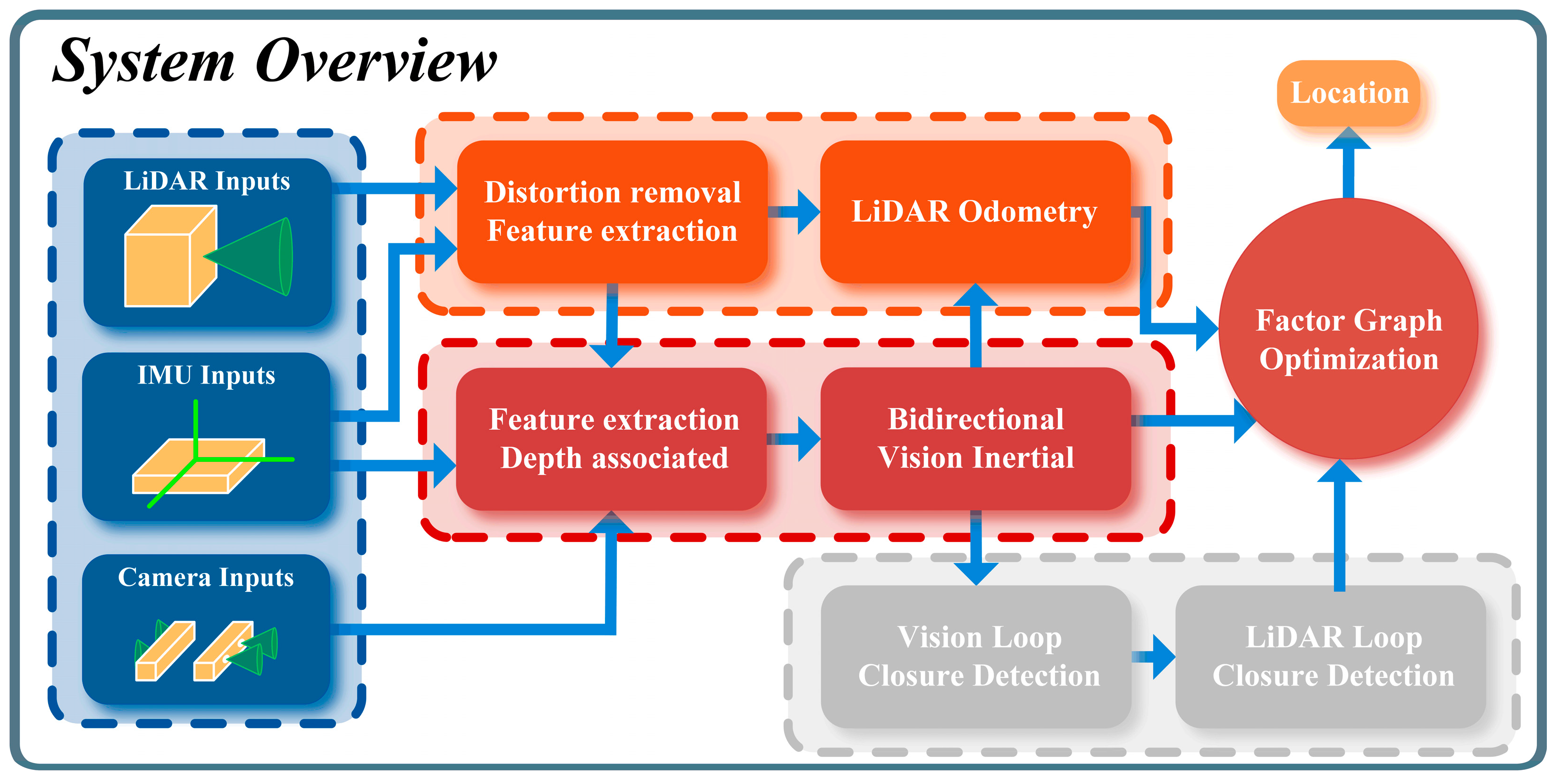
The system structure of the BV-LIO is shown in Figure 1. Firstly, visual and LiDAR feature points are extracted separately, and the monocular depth information of visual features is restored using 3D LiDAR points or visual geometric triangulation. Then, the LiDAR-assisted monocular vision is initialized, and the forward and backward bidirectional vision is tightly coupled with IMU for optimization and weighted fused into the visual inertial, which serves as a prior estimate to assist the LiDAR odometry for high-precision position and pose estimation. The visual odometry is obtained by weighted fusion and then given as a prior estimate to obtain the LiDAR odometry for high-precision pose estimation. Finally, loop closure detection and verification and joint factor graph optimization are performed to further improve the accuracy of pose estimation.

3.2. Depth Correlation and Initialization of 3D LiDAR and Bidirectional Vision

The bidirectional front and rear vision system are developed based on the VINS-Mono [24] framework, which performs adaptive mean histogram processing on input images to enhance image contrast and clarity. Harris corner features are then extracted from these images. The KLT optical flow tracking algorithm is used to track feature points from the previous frame. Feature points that are tracked most frequently are retained, and the distribution of feature points across the entire image is homogenized.

The extraction of LiDAR feature points is based on the curvature of the LiDAR point, calculated for the undistorted LiDAR point cloud. The curvature of each LiDAR point is obtained by the square root of the sum of the squared distance deviations between the five points before and after the current point. If the points near the LiDAR point are approximately on the same spherical surface, the curvature calculation should be close to 0.

$$Curvature\left[i\right]={\left(\sum _{t=i-5}^{t=i+5}\left(Range\left[t\right]-Range\left[i\right]\right)\right)}^2$$

(1)

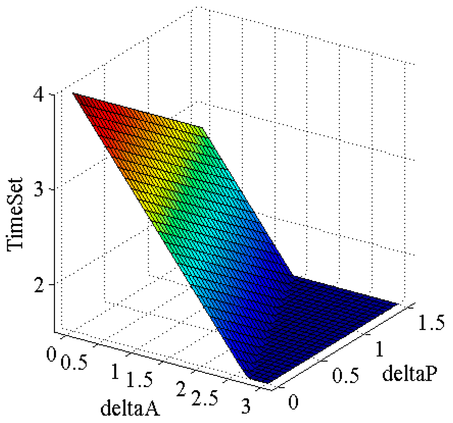
IMU pre-integration and de-distortion are performed on each frame of LiDAR point cloud, and the distortion-removed point clouds are accumulated into the local point cloud set. The local point cloud set is built by stacking sparse point clouds, retaining those in the recent time range, and discarding older data to obtain a newer, denser depth point cloud set for comparison with images. If the time window for the local point cloud collection is set too large, the maintained point cloud collection will become denser. But due to different timestamps of point clouds in the local collection, depth information associated with visual feature points may be blurred if rotation or translation increments are large over a short time, resulting in incorrect depth association. If the time window is too small, the maintained local point cloud set will be too sparse, possibly resulting in fewer or no LiDAR points associated with visual feature points meeting the conditions, causing depth association failure. As shown in Equation (2) and Figure 2, the time window is updated according to the rotation and translation increments of the mobile platform, dynamically maintaining the local point cloud, and demonstrating good applicability and reliability for mobile platforms of varying speeds.

$$Timeset=Tmax\ast \left(1-\left(\mu \ast {\displaystyle \frac{deltaA}{Amax}}+\eta \ast {\displaystyle \frac{deltaP}{Pmax}}\right)\right)$$

(2)

$Timeset$ is the length of time for the maintenance of the local point cloud set, $Tmax$ is the maximum value of $Timeset$, which is set to 4.0 s by default. $\mu$ and $\eta$ are the proportional coefficients of rotation increment $deltaA$ and translation increment $deltaP$, respectively. The default values are 0.7 and 0.3. $Amax$ and $Pmax$ are the angle increment and rotation increment maximum, respectively, with value defaults of 3.0 and 1.5.

Depth calculation for visual feature points is achieved through four steps:

• Convert the LiDAR local point cloud set to the camera coordinate system and project visual feature points and LiDAR depth points onto a unit sphere centered on the camera.
• For each visual feature point, we construct a 2D k-d tree using the spherical coordinates (azimuth and elevation) of all LiDAR depth points, with the feature point’s coordinates on a unit sphere as the reference. Subsequently, we perform a nearest neighbor search within this k-d tree to identify the three closest LiDAR depth points to the given visual feature point.
• If the maximum distance between the three lidar depth points is greater than 1.5 m, there is no matching information in the LiDAR local point cloud set for the visual feature point. The monocular triangulation method must be used to restore the depth information. Otherwise, proceed to step 4.
• Combine the three nearest LiDAR depth points and obtain the feature point’s depth value through interpolation calculation.

Both the front and rear cameras use this method to recover depth information for visual feature points.

In the system initialization stage, we first utilize IMU data to perform integration, providing a rough estimate of the robot’s initial pose to assist in the initialization of the LiDAR–inertial module. Once the LiDAR–inertial module is initialized, it supplies the state variables and bias parameters for the monocular vision system. During the visual initialization phase, if each image within the sliding window has corresponding LiDAR odometry prior information, we directly use this information to update the visual state variables and bias parameters. Otherwise, we initialize the camera pose using pure visual Structure from Motion (SFM) and align it with the IMU data to reduce uncertainty. Data from the front and rear cameras, after temporal synchronization and spatial calibration, jointly participate in the SFM and Bundle Adjustment (BA) optimization process within the sliding window. This integration provides richer visual information, enhancing the accuracy and robustness of the initialization. Through these steps, we effectively achieve the collaborative operation of the front and rear cameras, improving the stability and precision of the initialization.

3.3. Pose Estimation Method

3.3.1. Bidirectional Visual–Inertial Tightly Coupled Nonlinear Optimization

The visual–inertial module of the experimental platform in this paper includes front and rear vision. High-frequency, high-precision IMU odometry serves as an a priori estimation, tightly coupled with front and rear bidirectional vision. Visual odometry results from weighted fusion of the estimated states, avoiding reduced algorithm localization accuracy and robustness due to missing single visual features or tracking failure under weak texture or fast motion conditions.

In operation, the algorithm continuously receives sensor data. If all sensor measurements are considered, the computation required for data preprocessing and optimization is excessive. To reduce computation, image keyframe data is processed through a sliding window optimization method. Only keyframes within the window are considered in the optimization. Essentially, the visual–inertial tightly coupled nonlinear optimization problem is to find the Jacobian and covariance matrices of vision and IMU pre-integrations. As shown in Formula (3), the state vector to be optimized includes the IMU state in the sliding window: PVQ (position, velocity, rotation), bias, and the inverse depth of external parameters from the camera to the IMU and landmark points.

$$\begin{gathered} \chi =\left[x_n,x_{n+1},L,x_{n+N},x_c^b,{\lambda }_m,{\lambda }_{m+1},L,{\lambda }_{m+M}\right] \\ { x}_i=\left[p_{b_i}^w,q_{b_i}^w,v_{b_i}^w,b_a,b_g\right],i\in \left[n,n+N\right] \\ { x}_c^b=\left[p_c^b,q_c^b\right] \end{gathered}$$

(3)

In the above formula, ${\mathbf{x}}_i$ represents the IMU state corresponding to the frame image, ${\mathbf{p}}_{b_i}^w$, ${\mathbf{q}}_{b_i}^w$, and ${\mathbf{v}}_{b_i}^w$ represent the position, direction, and velocity, respectively, ${\mathbf{b}}_a$ and ${\mathbf{b}}_g$ represent the offset of the accelerometer and gyroscope, respectively. ${\lambda }_m$ represents the inverse depth of m-th 3D feature point, $\mathrm{n}$ represents the starting index of the IMU state variable in the sliding window, $\mathrm{N}$ represents the number of keyframes contained in the window, $\mathrm{m}$ represents the starting index of the feature state variable of the point in the window, $\mathrm{M}$ represents the feature point number in the window, and ${\mathbf{x}}_{\mathrm{c}}^{\mathrm{b}}$ represents the external parameter from the camera to the IMU.

To solve the nonlinear optimization problem by minimizing the sum of multiple errors, the cost function to be constructed is shown in Formula (4):

$$\underset{\chi }{\mathit{min}}\left\{ {‖r_p-H_p\chi ‖}^2+\sum _{k\in B}{‖r_B\left({\widehat{z}}_{b_{k+1}}^{b_k},\chi \right)‖}_{P_{b_{k+1}}^{b_k}}^2+\rho \sum _{\left(i,l\right)\in C}{‖r_C\left({\widehat{z}}_l^{c_i},\chi \right)‖}_{P_l^{c_i}}^2 \right\}$$

(4)

Among it, $r_B({\widehat{z}}_{b_{k+1}}^{b_k},\chi )$ represents the IMU residual term, $r_C({\widehat{z}}_l^{c_i},\chi )$ represents the visual observation residual term, and $\rho$ is the robust kernel function.$\{r_p,H_p\}$ is a marginalized prior constraint term, which can retain the influence of inter-frame constraints on the current state.

3.3.2. LiDAR Odometry Based on Bidirectional Visual–Inertial Odometry

LiDAR odometry only uses keyframes and ignores the rest. A sliding window-based method maintains corner and plane feature maps in combination with LiDAR keyframes to reduce computational complexity. Taking relatively high frequency visual odometry or IMU estimates as prior estimates, LiDAR odometry is obtained by minimizing the distance from detected line-surface features to the feature map. The prior estimate uses visual odometry at a higher priority. The visual–inertial subsystem is prone to failure due to insufficient tracked feature points in environments with fast motion, poor lighting, or missing textures. When a single visual sensor fails, another module can still work normally, enabling accurate IMU bias estimation and avoiding bias errors affecting pose estimation. Conditions for determining vision sensor failure include too few tracked feature points, excessive bias, excessive rotation increment, or excessive vehicle speed. If failure conditions are met, vision reinitialization is performed. If both front and rear bidirectional depth vision systems fail, LiDAR odometry does not use visual odometry as prior data for estimation. For the corner feature corresponding to the current LiDAR frame, the k-Nearest Neighbor method of the PCL library is used to find five corners adjacent to the point in the corner feature map. If the distances between these five points and the reference point are all less than the threshold and are approximately collinear, it is considered that the corner feature matches the corner feature map. The residual calculation of the corner point is essentially to find the distance from the point to the corresponding feature line on the feature map.

For the plane feature corresponding to the current LiDAR frame, the nearest five points in the plane feature map must be identified. If the distances between these five points and the reference point are all less than the threshold and approximately coplanar, the plane feature is deemed to match the plane feature map. Residual calculation for the plane feature point essentially involves finding the distance from the point to the target plane feature on the feature map.

For the two types of feature points used in matching, the Jacobian matrix is calculated, and the distance from the feature point to the target line feature and the target plane feature is used as the observation value. The Gauss–Newton equation is established, and the current pose is iteratively optimized to obtain the LiDAR odometry.

3.4. Loop Closure Detection and Factor Graph Optimization

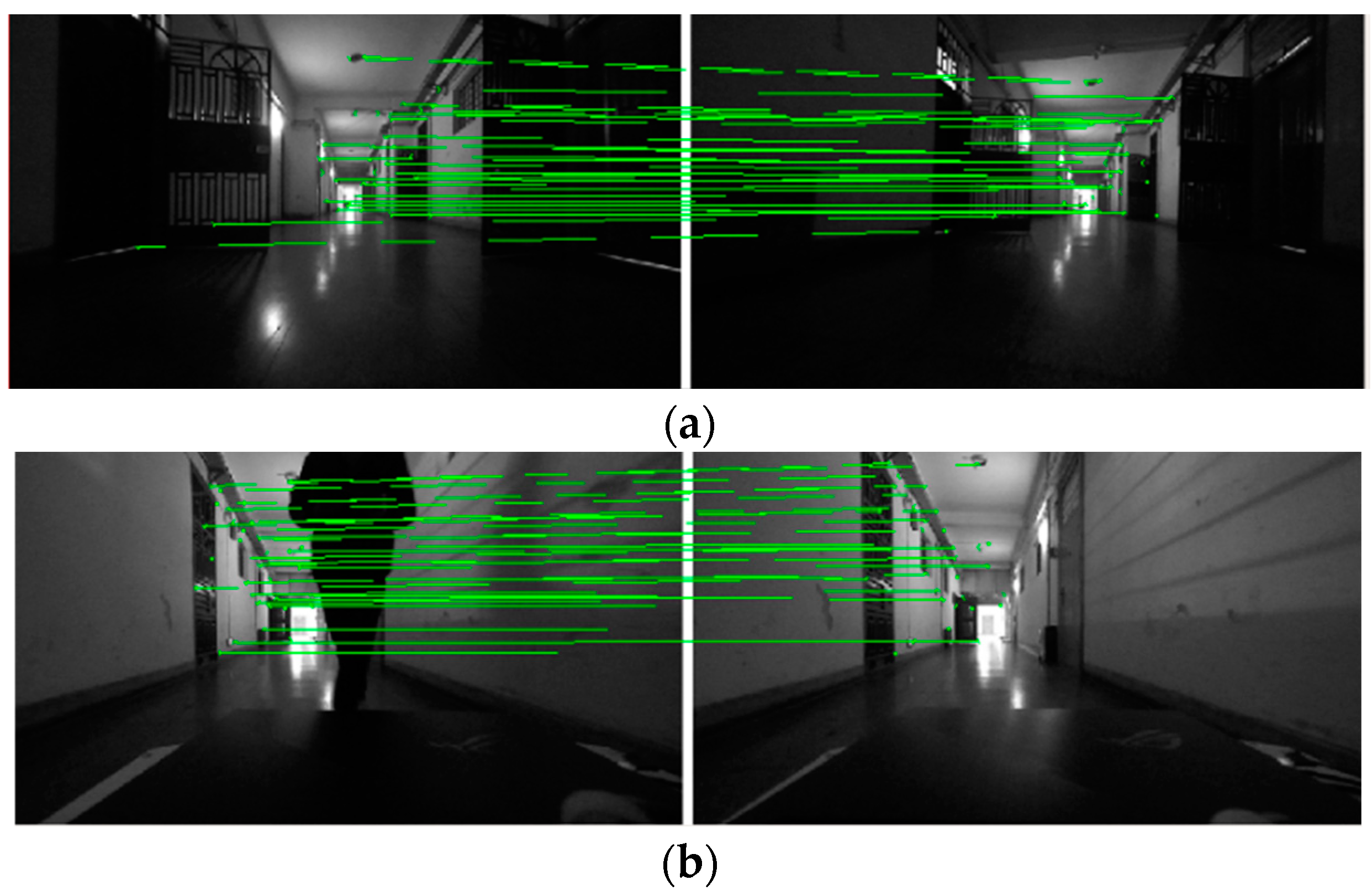
The visual loop closure detection utilizes the DBoW2 method. When a new image keyframe is added, all feature points of the image are described by the Brief feature descriptor. The similarity score between the current image keyframe and the bag of words is calculated, and the loop closure visual keyframe is returned according to the similarity. The visual part adopts bidirectional cameras to detect loop closure simultaneously, and the detection effect is shown in Figure 3. To improve the overall algorithm efficiency, the selection of visual loop closure frames requires checking for temporal and spatial consistency, avoiding situations where the front and rear cameras detect loop closure simultaneously or continuously detect loop closure within a short period.

In actual scenes, when forward or backward visual features are missing, making loop closure detection challenging from one viewpoint, the loop closure detection results from another viewpoint camera can compensate for this deficiency, enabling the optimization of historical keyframe poses. Upon successful visual loop detection, timestamps for the current and loop closure moments are obtained. Corresponding LiDAR keyframes are identified in the historical LiDAR keyframe queue. Local feature point clouds are constructed for each keyframe and registered. If registration succeeds, the visual loop closure is validated.

To improve the detection success rate, a 3D Kd-tree is constructed using positions of all LiDAR keyframes in history. The Kd-tree is searched according to the current LiDAR keyframe pose at regular intervals to find the nearest neighbor. If the position distance between the current LiDAR keyframe and the adjacent frame is less than the set threshold, the adjacent frame is used as the LiDAR keyframe corresponding to loop closure, realizing LiDAR loop closure detection.

GTSAM is a commonly used optimization library in factor graph optimization, including the algorithms of iSAM, iSAM2 and the optimization of Bayesian tree. It is used in the field of robotics for smooth graph construction and solving problems in SLAM and SFM.

This section further optimizes the robot posture based on the factor graph. As the algorithm’s runtime increases, accounting for all keyframes’ postures and characteristics simultaneously reduces computational efficiency and can even preclude real-time execution. To avoid optimizing numerous feature points, odometry constraints are constructed using pose transformation relationships between keyframes from front and rear bidirectional vision. For adjacent LiDAR keyframes, a LiDAR odometry factor is constructed based on their position and pose transformation relationship; for adjacent visual keyframes, a visual odometry factor is similarly constructed. For loop closure keyframes, the pose transformation relationship between the current frame and the loop closure keyframe is obtained via ICP registration. A loop closure factor is then constructed from this. The odometry factor can be uniformly defined as:

$$arg\underset{T}{\mathit{min}}\left\{\sum _{\left(i,j\right)\in O}{‖r_{ij}‖}^2+\sum _{\left(i,j\right)\in V}{‖r_{ij}‖}^2+\sum _{\left(i,j\right)\in L}{h(‖r_{ij}‖}^2)\right\}$$

(5)

The problems are solved using iSAM2, yielding an optimized LiDAR keyframe pose. Per IMU data between the current and previous LiDAR keyframes, the IMU pre-integration and offset factors are calculated and added for further optimizing the current LiDAR keyframe status: pose, speed, and IMU offset. Optimizing IMU bias mitigates pre-integration drift.

For the optimized LiDAR odometry, the IMU pre-integration is performed again for the IMU data after the current frame time with the latest IMU offset. The improvement of IMU pre-integration accuracy can provide more accurate initial value estimation for LiDAR odometry. For the IMU data after the corresponding time of the optimized LiDAR odometry, based on the corresponding state and bias at that time, the IMU state at each time is calculated according to the IMU pre-product component, and the IMU odometry at each time is obtained, to realize the parallel estimation of the visual odometry, LiDAR odometry, and IMU odometry. IMU odometry is used as the initial value of position, and pose estimation of visual odometry, visual odometry, and IMU odometry are used as the initial value of LiDAR odometry matching, and vision and LiDAR limit the deviation for IMU. Under the condition of limited offset, the IMU odometry is very accurate. The architecture of the algorithm in this paper has strong extensibility. It can combine other odometry factors and global location factors to add more constraints.

4. Experiments and Analysis

To verify the accuracy and robustness of the proposed SLAM algorithm, we tested it on various public datasets. In addition, to verify the effectiveness of the proposed SLAM algorithm in weak-texture scenes, we built a mobile platform and manually controlled the robot to move in real scenes.

4.1. Pose Estimation Accuracy Verification Experiment

To verify the accuracy and robustness of the proposed pose estimation method, we conducted experiments on the public datasets KITTI and M2DGR. Due to the lack of rear-view cameras in the KITTI dataset, we conducted experiments using the left and right grayscale cameras. Before using the dataset, we converted it into ROS rosbag format using the kitti2bag tool, based on the sensor’s intrinsic and extrinsic parameters, ground truth trajectories, timestamps, and raw sensor data, for subsequent trajectory evaluation. Similarly, the M2DGR dataset is also provided in rosbag format, with sensor data published through ROS topics. Additionally, the M2DGR dataset includes both front and rear camera data.

We compared our algorithm with LiDAR-based Algorithm (LeGO-LOAM and LIO-SAM), Visual-based Algorithm (VINS-Mono and ORB-SLAM3-stereo), and a SLAM algorithm using LiDAR-Vision fusion. As shown in

Table 1. Pose Accuracy Comparison Experiment Based on KITTI and M2DGR Public Datasets with LiDAR-based Algorithm and Visual-based Algorithm.

RMSE APE1/APE2 (m)	LeGO-LOAM	LIO-SAM	VINS-Mono	ORB-SLAM3-Stereo	BV-LIO- No Loop	BV-LIO- with Loop
KITTI_05	1.033/1.131	1.016/1.831	15.080/29.808	0.402/2.416	--/2.055	0.796/1.501
KITTI_08	2.845/3.282	4.376/5.595	7.185/8.530	2.849/2.847	--/8.065	2.674/4.238
KITTI_10	1.973/1.968	1.631/1.896	5.422/5.420	1.477/1.673	--/1.829	1.522/ 1.676
M2DGR_02	4.390/4.697	3.262/3.462	43.997/42.753	98.007/98.011	--/2.757	2.545/2.709
M2DGR_04	1.760/1.807	0.867/0.898	X	X	--/1.858	0.759/1.863
M2DGR_06	1.013/1.060	0.371/0.387	115.092/125.669	40.512/40.493	--/0.789	0.411/0.433
Average	2.169/2.324	1.921/2.345	37.355/42.436	28.649/29.088	--/2.892	1.451/2.070

Note: Where X indicates that the algorithm fails the test under the corresponding dataset, the algorithm cannot be initialized normally, or the problem of feature tracking loss is very serious, resulting in the normal tracking duration being less than half of the total duration of the dataset.

, there are the pose accuracy and comparison results of each open-source SLAM algorithm based on the public dataset and running on the same computing platform. The format of the data elements in the table is: (APE1/APE2), where APE1 is calculated based on the historical poses of all keyframes after loop closure optimization, which is called the absolute position error of the optimized trajectory; APE2 is calculated based on the real-time output keyframe poses, called the absolute position error of the real-time pose.

By analyzing specific data in Table 1, our algorithm reduces average real-time pose error by 10.93% and 11.70% compared to LeGO-LOAM and LIO-SAM. It reduces average pose error by 33.10% and 24.44%. Compared to VINS-Mono and ORB-SLAM3, our algorithm’s average pose error is close to ORB-SLAM3 on both KITTI datasets. Under the M2DGR dataset, our algorithm runs stably even with missing visual features or lost tracking in scenes with poor texture and insufficient light. Its average pose error is much lower than VINS-Mono and ORB-SLAM3, which can stably output high-precision pose data. Although both algorithms employ adaptive histogram equalization to process images under low-light conditions, they still fail to extract sufficient feature points in these dark scenes, making tracking challenging. As shown in Figure 4, due to poor lighting in the scene, many of the detected feature points come from distant streetlights or building lights. Even if visual initialization is successful, the subsequent operation may suffer from insufficient feature points, tracking failures, and mismatches, leading to significant errors. In severe cases, the algorithm may fail completely, necessitating reinitialization. Additionally, due to the overly sparse textures and vast open space in the M2DGR_04 scenario, the visual SLAM algorithms compared in this study could not complete initialization.

Additionally, with the loop closure detection enabled in our algorithm, the average position error of real-time pose estimation is significantly reduced from 2.892 m to 2.070 m compared to the open-loop state. This improvement is mainly due to the effective reduction of cumulative error through loop closure correction, enhancing the accuracy of subsequent pose estimations. As shown in Figure 5, the trajectory is plotted and evaluated using the EVO tool. GT represents the ground truth trajectory, and BV-LIO represents our proposed algorithm.

To further verify the effectiveness and accuracy of the proposed algorithm, we compared it against a LiDAR-vision fusion SLAM algorithm that lacks semantic information. Based on algorithm performance, open-source status, and experimental data from original papers, we selected DEMO, DVL-SLAM, DV-LOAM, and the method proposed by Huang et al. for comparison. We used the KITTI dataset for evaluation and calculate pose error to measure performance.

Table 2. Pose Accuracy Comparison Experiment with LiDAR-vision fusion Algorithm.

Mean RPE (%)	DEMO	DVL-SLAM	Huang	DV-LOAM	BV-LIO- No Loop	BV-LIO- with Loop
KITTI_05	1.04	0.82	0.72	0.54	0.92	0.77
KITTI_08	1.24	1.32	1.27	0.89	1.27	1.14
KITTI_10	1.14	0.70	0.83	0.87	0.86	0.86
Mean	1.14	0.95	0.94	0.77	1.02	0.92

presents a comparison of pose accuracy between our algorithm and other LiDAR-visual fusion algorithms. The errors for comparison algorithms result from open-loop conditions and directly reference experimental results in corresponding original author papers.

The positioning accuracy of our proposed algorithm in open loop falls between that of DEMO and DVL-SLAM, with an average relative position error of 1.02%. KITTI only includes camera data from a forward-facing perspective, and the experimental data for the comparison algorithms in Table 2 comes from the authors’ original papers, not from experiments run on the same computing platform. The experimental results confirm the effectiveness and accuracy of our proposed algorithm.

To validate the effectiveness of bidirectional vision, we also conducted an ablation study using only forward vision, as shown in

Table 3. Ablation Experiment for Bidirectional Vision.

RMSE APE1/APE2 (m)	BV-LIO w/o Rear-Vision	BV-LIO
M2DGR_02	2.863/3.062	2.545/2.709
M2DGR_04	0.807/1.938	0.759/1.863
M2DGR_06	0.432/0.445	0.411/0.433
Average	1.367/1.815	1.238/1.668

. The experimental results indicate that bidirectional vision significantly improves pose estimation accuracy compared to unidirectional vision.

4.2. Validation Experiment on Our Dataset

In this section, this paper records the dataset in the inspection scene through the mobile robot built by ourselves and verifies the proposed algorithm. The mobile robot and sensor suite are shown in Figure 6a.

The LiDAR used is a Leishen C32-151A mechanical LiDAR, with a ranging accuracy of ±3 cm, a horizontal field angle of 360°, and a horizontal angle resolution of 0.18° (scanning frequency of 10 Hz). The front and rear cameras are ZED2 cameras. ZED2 is a high-definition, high-frame rate binocular depth camera made by Stereo labs in the United States. It has built-in high-precision IMU, magnetometer, barometer, and other sensors. The 6-axis pose position accuracy is 1 mm, and the direction accuracy is 0.1°. We uniformly use the IMU data built into the forward-facing camera for visual inertia odometer (VIO) calculations. A high-performance notebook computer is configured with an Intel i7-10870H processor, 16 GB of memory, and an Nvidia RTX 2060 graphics card. An embedded control board, designed and developed based on stm32f103, has functions of PWM output, IO acquisition, timer, and serial communication.

Due to the absence of GPS hardware for time synchronization, our multi-sensor system utilizes different methods for synchronizing data. The front-facing camera and IMU are synchronized via hardware, while the IMU, rear-facing camera, and LiDAR are synchronized using software timestamps provided by the ROS system. For sensor calibration, the IMU intrinsic parameters are calibrated using the imu_utils tool. The intrinsic parameters of the ZED2 camera, as well as the extrinsic parameters between the camera and IMU, are calibrated using the Kalibr tool. The extrinsic parameters between the 32-line LiDAR and the IMU coordinate system are calibrated using the LI-Calib tool developed by Zhejiang University. Based on these calibration results, we derive an initial estimate of the extrinsic parameters between the LiDAR and the camera. Using this estimate, we project the LiDAR point cloud onto the image. We then manually fine-tune the parameters using the dynamic_reconfigure package in ROS. Finally, we select several corresponding points and employ the PnP algorithm to achieve precise extrinsic calibration.

In this paper, the dataset is recorded in an indoor corridor scene with weak texture. To provide specific values for the experimental environment’s brightness, we used a lux meter to measure the light levels in the indoor corridor, which averaged between 40–60 lux. Additionally, the camera’s white balance, exposure, and gain were set to “auto” mode, ensuring that the camera automatically adjusts these parameters based on the scene’s brightness to capture clear images. The recorded information includes front and rear bidirectional cameras, 32-line LiDAR point clouds, and IMU data. The experimental environment is the weak texture environment of an indoor corridor with relatively dark lighting. In the process of remote control, the mobile platform zigzagged along the corridor, with many obvious acceleration and deceleration processes. The image in the camera’s field of view during the experiment is shown in Figure 6b.

Table 4. Indoor Environment Pose Estimation Accuracy Comparison Experiment Results.

Error (m)	LeGO- LOAM	LIO-SAM	VINS-Mono	ORB-SLAM3 -Stereo	BV-LIO -No Loop	BV-LIO -with Loop
X	0.062/0.067	0.029/−0.013	−0.017/0.327	0.744/0.327	--/−0.010	0.012/−0.024
Y	−0.015/−0.013	0.058/0.053	0.056/0.18	−0.219/−0.34	--/0.014	0.048/0.061
Z	0.02/−0.029	−0.1/−0.17	0.037/0.135	−0.009/−0.013	--/−0.283	−0.009/−0.012
Position	0.067/0.074	0.119/0.178	0.069/1.588	0.549/0.472	--/0.283	0.051/0.066
Lower	24.39%/ 10.81%	57.51%/ 62.98%	27.22%/ 95.84%	90.79%/ 86.00%	--/76.69%	--

shows the results of pose estimation in the indoor weak texture corridor environment. After many experiments, the average results are recorded. The X axis, Y axis, Z axis, and position error are measured by the relative position of the starting point and the end point. The algorithm BV-LIO in this paper only records the absolute position error of the real-time output pose in the open-loop state. The format of the data element in the table is: (E1/E2). The error E1 is calculated through the loop closure optimized posture, and the error E2 is calculated based on the real-time output posture. The results show that the performance of our proposed algorithm is significantly better than other algorithms under closed-loop conditions, with the largest improvement compared to ORB-SLAM3-Stereo, with E1 improving by 90.79% and E2 improving by 86.00%. Figure 7 shows the trajectory after global pose optimization.

5. Conclusions

We designed a pose estimation method based on bidirectional visual–inertial odometry with 3D LiDAR, comprising a bidirectional visual–inertial and a LiDAR–inertial module. It combines the efficiency of VIO and the accuracy of LiDAR frame map matching. The front and rear bidirectional vision is tightly coupled with the IMU to obtain two estimated states. Visual loop closure detection results are confirmed by the LiDAR–inertial module, reducing repeated and false detections. The factor graph is optimized by combining LiDAR odometry constraints, visual odometry constraints, IMU constraints, and loop closure constraints, yielding high-precision robust pose estimation. The proposed method avoids loop closure detection and feature missing due to limited single visual angle, enhancing system efficiency and robustness. It achieves high-precision robust pose estimation, holding great application value for mobile robots working.