Analyzing Thermal Environment Contributions and Driving Factors of LST Heterogeneity in Different Urban Development Zones

Abstract

Analyzing the impacts of urban landscape patterns on the thermal environment has become one of the key research areas in addressing urban heat islands (UHIs) and improving the living environment. A case study was carried out in Fuzhou, Fujian Province of China, and bi-temporal Landsat imagery was selected to calculate land surface temperature (LST), percent impervious surface area (ISA), and fractional vegetation cover (FVC). The urban area was further divided into three concentric urban zones, ranging from the city center to the urban periphery, based on urban development densities. The spatial pattern of LST and its variance were analyzed and compared between different zones and different dates. The thermal environment contribution of different zones was also quantified to indicate the change in urban landscape patterns resulting from urban expansion in different zones. Furthermore, Geodetector was used to explore the single factors and interaction factors controlling the spatial patterns of LST in each zone. The results showed that (i) urban expansion primarily increased in Zone 2 and Zone 3, and the areal proportion of high and sub-high LST areas increased from 56.11% and 21.08% to 62.03% and 32.49% in Zone 2 and Zone 3, respectively, from 2004 to 2021; (ii) the heat effect contribution of Zones 2 and 3 reached from 75.16% in 2004 to 89.40% in 2021, indicating that the increase in ISA with >LST_mean was more pronounced in Zone 3 and Zone 2 during the period; (iii) the driving factors of LST spatial distribution were regionally different because of the different landscape patterns, and the explanatory power for the heterogeneity of LST in Zone 1 was weaker than in Zone 2 and Zone 3 in the study area; (iv) the interaction of different factors had a higher explanatory power in the spatial distribution of LST than a single factor in each zone because the distributions of land cover types are heterogeneous in urban areas. The results of this study can be used to improve urban planning for urban ecology and UHI mitigation.

1. Introduction

The rapid urbanization process has resulted in an increasing impervious surface in urban and surrounding areas, further impacting the urban thermal environment [1,2]. It is obvious that city centers have higher land surface temperatures (LSTs) and experience higher LST heterogeneity than the surrounding suburbs in terms of rural–urban temperature differences, a phenomenon known as the urban heat island (UHI) effect [3,4,5,6]. Therefore, accurate analysis of the urban landscape pattern and thermal environment is important for mitigating the UHI and improving urban livability [7].

In urban areas, continuous percent ISA information with a value from 0% to 100% can reveal central business districts and urban residential areas with varying densities and landscape patterns, rural developed centers, and relatively undeveloped areas [8]. An increase in the percent ISA from 0 to 100% can result in increasing LST and UHI; inversely, FVC with a value increased from 0% to 100% can decrease LST and mitigate UHI [9]. Although some studies have indicated that urban landscape patterns or land-use types significantly affect LST, few studies have explored the different landscape patterns and thermal contributions of different urban development areas [1,10]. In order to effectively adapt to climate change, it is important to analyze the thermal contribution of different landscape patterns to urban functional zones and the entire urban area.

Impervious surface area (ISA) and vegetation cover are two crucial parameters in the analysis of LST and urban thermal patterns [6,11]. Urban expansion leads to vegetation area reduction, impervious surfaces increase, and alterations in regional climate [12,13]. To simulate the climatology of UHI phenomena corresponding to changes in urban landscape patterns, it is essential to extract the percentage of ISA and fractional vegetation cover (FVC) that capture the landscape evolution [9,14]. Landsat remote sensing imagery with a spatial resolution of 30 m × 30 m is commonly employed to generate urban landscape pattern data. Due to the mixed pixel problem, soft classification techniques, such as spectral unmixing, are typically used to extract sub-pixel information for characterizing urban land cover patterns and thermal environments [11,15].

To mitigate the UHI effect and adapt urban areas to climate change, it is crucial to understand how changes in ISA and vegetation cover, as well as their composition, contribute to urban LST [16,17,18]. Previous studies have shown that the percentage of ISA and FVC provide complementary information to hard-classified land cover types for analyzing the urban thermal environment [19,20,21,22,23].

Boosted regression trees, random forest, and convolutional neural networks have been proven to be effective in detecting the effect of urban landscape patterns on LST [24,25]. However, the effects and spatial distribution of urban ISA and vegetation on the thermal environment need to be further analyzed, particularly in areas with varying ISA and vegetation densities due to different stages of urban development [2,26,27]. Therefore, it is necessary to analyze the impact of variations in fractional covers of ISA and vegetation on the thermal environment, as well as the spatial heterogeneity or agglomeration of LST in different urban development areas [2,28,29].

The spatial heterogeneity of LST is a common geographical phenomenon in urban expansion [2,28,30]. Analysis of the spatial distribution and spatial heterogeneity or agglomeration of the urban thermal environment in the urbanization process can help planners understand characteristics such as the direction and degree of urban expansion and further promote the healthy development of urbanization through reasonable urban planning [31,32,33]. Geodetector has been applied to analyze the factors controlling the spatial patterns of various geographical phenomena [34]. At present, there are few studies to measure the spatial heterogeneity of LST resulting from urban expansion and its driving forces. In order to effectively cope with urban climate change, it is necessary to analyze the connection between the heterogeneity characteristics of LST and their influencing factors, which are vital for the prevention and remediation of the negative impact of the UHI [14,35]. In this study, Geodetector was used to reveal the spatial influence of some factors on LST in different urban development categories through driving forces analysis.

This study selected a study area to explore the spatial influence of urban landscape patterns on the thermal environment. A fully constrained linear spectral unmixing method was used to extract subpixel fractional cover data. Two Landsat images were selected to quantify the impact of urban landscape patterns on the urban thermal environment and the factors controlling the spatial heterogeneity of urban LST. The objectives of this study were to (1) investigate the characteristics of urban landscape patterns and LST in different urban development areas; (2) explore the variations the thermal environment by analyzing and comparing the heat effect contributions based on different development zones and different dates; (3) reveal the internal regularities affecting the spatial pattern of LST by investigating and comparing the driving factors of LST spatial distribution in urban different development areas. The results of this study can provide information for urban planners on how to mitigate the UHI effect through rational landscape design and urban management.

2. Materials and Methods

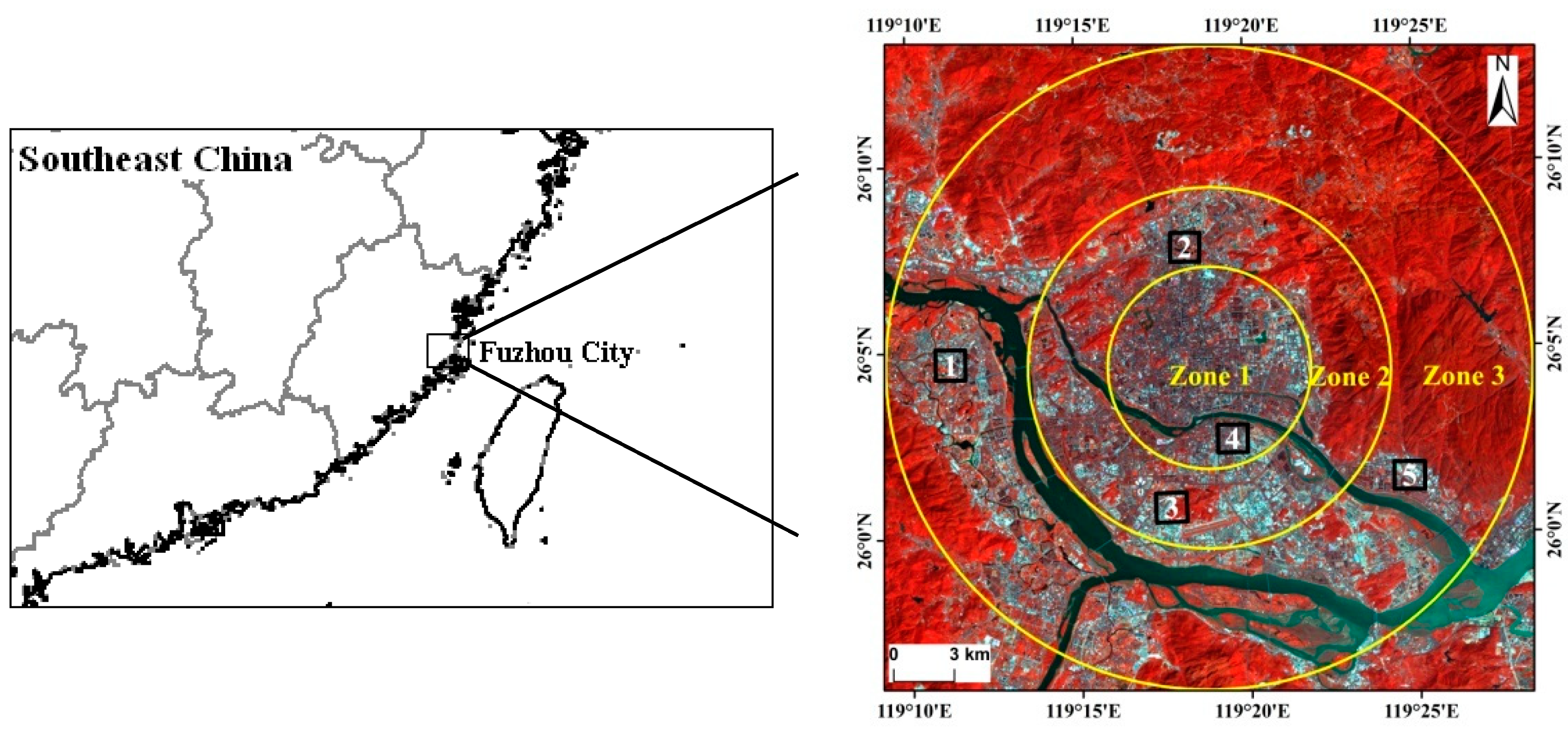
2.1. Study Area and Data

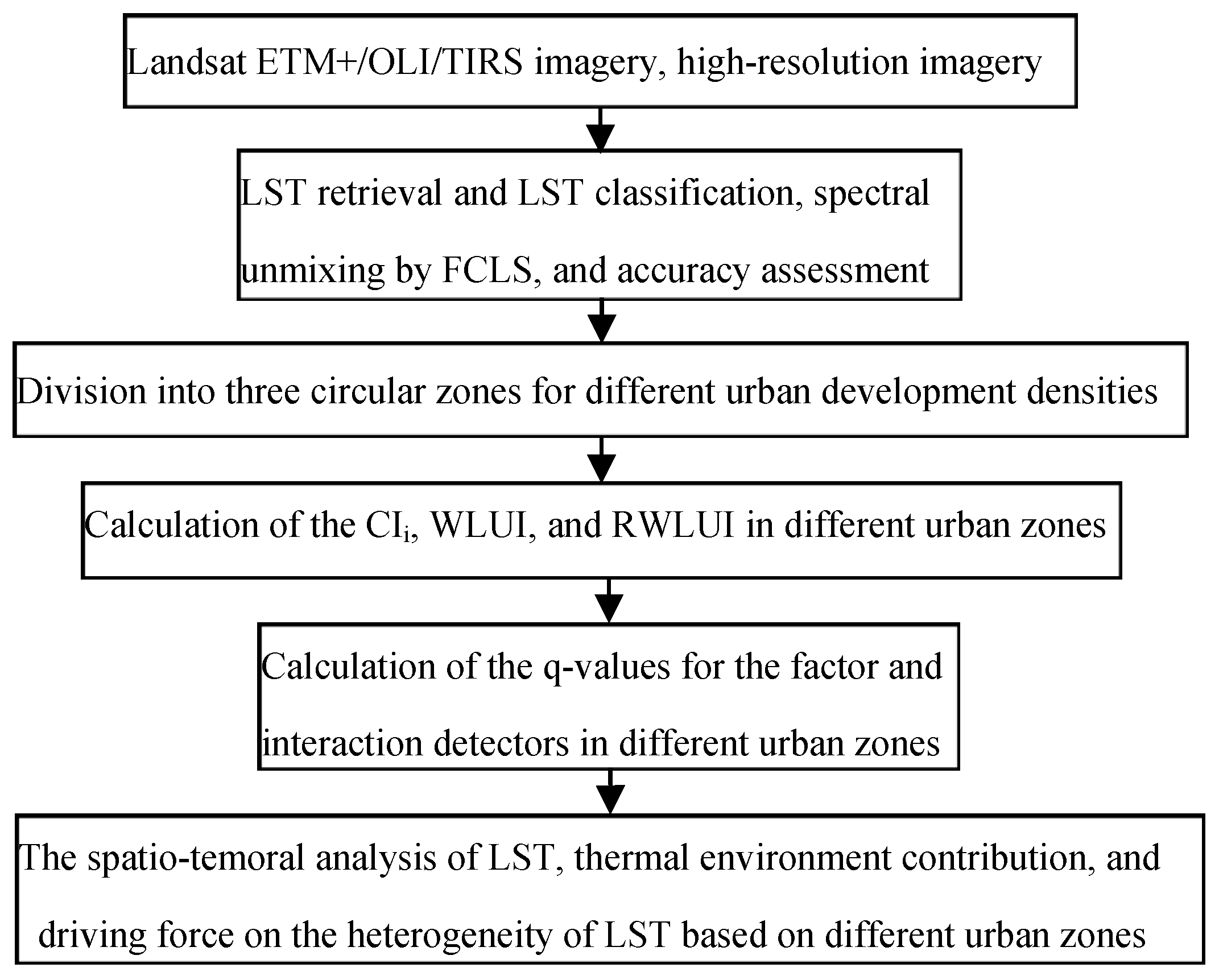
Fuzhou, the capital city of Fujian Province in southeastern China, was selected as the study area (Figure 1). Fuzhou has experienced rapid urban expansion due to a significant increase in population over the last 30 years. This urban expansion entailed a transformation of land cover types, shifting from natural surfaces to impervious surface areas. These changes in the urban landscape pattern have led to alterations in thermal properties, surface radiative properties, and ecosystems. The city is surrounded by mountains and is located in a subtropical humid climate zone. The vegetation in the region is predominantly evergreen, and the fraction of vegetation cover remains nearly constant throughout different seasons. Fuzhou experiences hot summers, while winters have a mild climate, and variations in climate during spring, autumn, and winter are minimal.

Bi-temporal, cloud-free Landsat images were utilized in this study, including a Landsat 7 ETM+ image (acquired on 12 September 2004) and Landsat 8 Operational Land Imager (OLI) and thermal infrared sensor (TIRS) images (acquired on 27 September 2021). Additionally, bi-temporal, high-spatial-resolution images (acquired in 2004 and 2021, respectively) with a 4 m spatial resolution obtained from the Google Earth website were used to assess the accuracy of the percent ISA and FVC derived through spectral unmixing from Landsat imagery. The land surface reflectance of visible and near-infrared bands of Landsat data was derived using the FLAASH model in ENVI.

To effectively analyze and compare urban landscape and thermal patterns in different development areas, the study area was divided into three circular zones (Zone 1, Zone 2, and Zone 3) from the city center to peripheral urban areas, representing different urban development densities (as delineated by yellow lines in the right figure of Figure 1). Zone 1 comprises the urban core area with high development density, Zone 3 represents an area with low development density in the peripheral urban areas, and Zone 2 encompasses an area with medium development density situated between Zone 1 and Zone 3. Zone 2 was not considered part of the urban area in 2004 but was included in the urban extent in 2021 due to urban expansion. These three divided zones exhibited distinct development densities. The data generated from zonal statistics aid in understanding the thermal environment contributions of various urban development areas and the driving forces behind the spatial heterogeneities of LST more accurately.

2.2. Methods

The methodology for this study consists of four main steps. The first step includes LST retrieval and fractional cover retrieval by spectral unmixing. The second step includes LST classification and accuracy assessment of subpixel fractional covers. The third step explores thermal environment contribution based on different urban zones; this step includes the calculation of the thermal environment contribution index (CI_i), the weighted LST unit index (WLUI), and the regional weighted LST unit index (RWLUI). The fourth step analyzes the driving forces of the LST heterogeneity at different zones by calculating q-values. A flowchart of the study is illustrated in Figure 2.

2.2.1. LST Retrieval and LST Classification

Bi-temporal LST data were retrieved from Landsat 7 ETM+ and Landsat 8 TIRS/OLI images. The radiative transfer equation was employed to derive LST from the Landsat data. Firstly, top-of-atmosphere (TOA) radiance was calculated from the bi-temporal Landsat images through radiometric calibration. Subsequently, TOA radiance values for visible/near-infrared bands were converted to surface reflectance using the atmospheric correction tool MODTRAN 4.1. Simultaneously, TOA radiance values for thermal infrared bands (Band 6 of Landsat 7 ETM+ and Band 10 of Landsat 8 TIRS) were transformed to surface-leaving radiance (L_T) by applying the atmospheric correction tool MODTRAN 4.1 and inverting Planck’s law [36]:

$${\mathrm{L}}_{\mathrm{T}}={\displaystyle \frac{{\mathrm{L}}_{\mathsf{\lambda }}{-\mathrm{L}}_{\mathsf{\mu }}-\mathsf{\tau }\left(1-\mathsf{\epsilon }\right){\mathrm{L}}_{\mathrm{d}}}{\mathsf{\tau }\mathsf{\epsilon }}}$$

(1)

where L_λ is the TOA radiance image for the thermal infrared band, Lμ, L_d, and τ are the upwelling radiance, downwelling radiance, and transmission, respectively. The atmospheric correction tool MODTRAN 4.1 was used to estimate the values of L_μ, L_d, and τ. ε is the surface emissivity calculated according to the methods in [37,38].

Finally, LSTs were calculated by the Landsat-specific estimate of the Planck curve [39]:

$$\mathrm{LST}={\displaystyle \frac{{\mathrm{k}}_2}{\ln \left(\right({\mathrm{k}}_1/{\mathrm{L}}_{\mathrm{T}})+1)}}$$

(2)

where LST is the temperature in Kelvin (K), and k₁ and k₂ are the pre-launch calibration constants. For Landsat 7 ETM+, k₁ = 666.09 W/(m²srμm) and k₂ = 1282.71 K. For TIRS Band 10, k₁ = 774.89 W/(m²srμm) and k₂ = 1321.08 K.

The resolution of the visible/near-infrared bands of Landsat 7 ETM+ image and Landsat 8 OLI image is 30 m while Band 6 of Landsat 7 ETM+ image and Band 10 of Landsat 8 TIRS image) are collected at a resolution of 60 m and 100 m, respectively; the thermal infrared data were resampled to 30 m in this study. Figure 3a,b are LST retrieved from the ETM+ image acquired on 12 September 2004 and LST retrieved from the TIRS image acquired on 27 September 2021, respectively.

The LST of the same area may show some differences between different dates even in the same season because the multi-temporal images were acquired in different atmospheric conditions. In order to reduce the influence of such LST fluctuations, the four-level LST classes were created by adding or subtracting standard deviation (SD) from mean LST of the whole study area:

LST₁: LST ≤ (LST_mean−2SD)
LST₂: (LST_mean−2SD) < LST ≤ LST_mean
LST₃: LST_mean < LST ≤ (LST_mean + 2SD)
LST₄: LST > (LST_mean + 2SD)

(3)

The LST increases from LST₁ to LST₄, and the LST₄ area is defined as a high temperature area. The classification of four-level LST can be used to analyze the evolution of the thermal environment. Four LST classes are calculated as in Equation (3) and shown in Figure 3c,d.

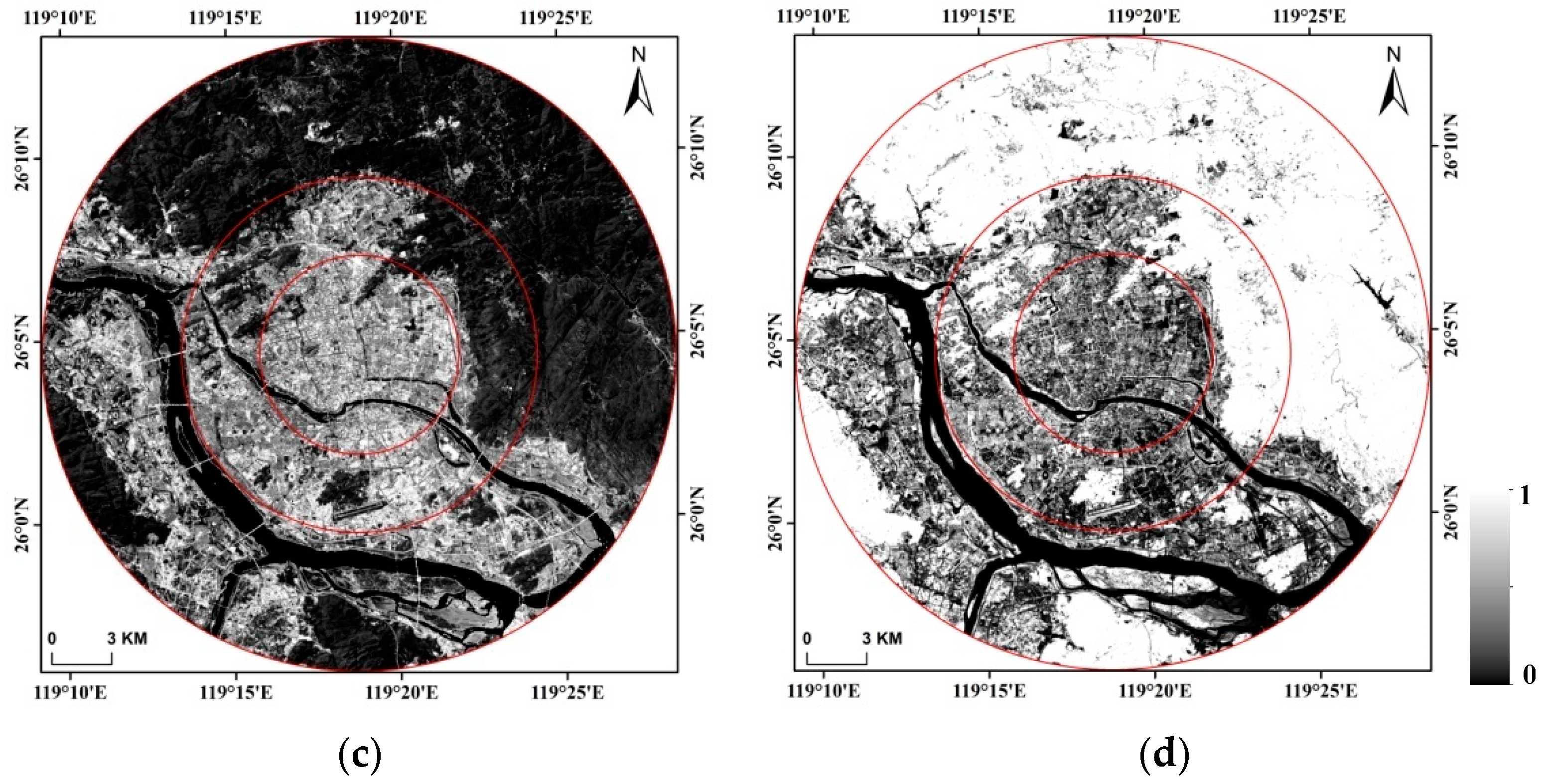
2.2.2. Percent ISA and FVC Derived by Spectral Unmixing of Fully Constrained Least Squares and Accuracy Assessment

Continuous percent ISA information can reveal areas of urban development with varying densities and patterns. As one of the soft classification methods, linear spectral unmixing by fully constrained least squares (FCLS) is frequently adopted to extract sub-pixel land cover types for remote sensing imagery, especially for Landsat imagery. In this study, FCLS was used to extract sub-pixel ISA and vegetation from Landsat imagery. The FCLS method assumes that the reflectance of each pixel at each band is a linear combination of the reflectance of all endmembers within the pixel [40]. The spectral reflectance in band i can be described as follows:

$${\mathrm{R}}_{\mathrm{i}}={\sum }_{\mathrm{k}=1}^{\mathrm{n}}{\mathrm{f}}_{\mathrm{k}}{\mathrm{r}}_{\mathrm{i}\mathrm{k}}+{\mathsf{\epsilon }}_{\mathrm{i}}$$

(4)

$$\sum _{\mathrm{k}=1}^{\mathrm{n}} {\mathrm{f}}_{\mathrm{k}}=1{\mathrm{f}}_{\mathrm{k}}\ge 0 \mathrm{f}\mathrm{o}\mathrm{r} \mathrm{k}=1,2,3,\dots ,\mathrm{n}$$

(5)

where n is the number of endmembers, f_k the fraction of endmember k within the pixel, r_ik the reflectance of endmember k in band i, and ε_i is the residual error for band i. Equation (5) provides the constraint conditions for spectral unmixing. The fractions of one pixel must sum to 1, and all fractions must be ≥0.

Firstly, the water body was masked out from the images of the study area, and two-dimensional spectral mixing spaces were used to extract endmembers of vegetation, impervious surfaces (high- and low-albedo impervious surfaces), and soil. Then, applying the FCLS technique, the fractional cover of each component was estimated by Equations (4) and (5). Finally, the high- and low-albedo ISA classes were aggregated to total percent ISA.

Figure 4 displays the fractional covers of ISA and vegetation derived by FCLS from the Landsat data for 2004 and 2021. Because soil areas are limited and primarily distributed alongside the river, and soil does not have a significant effect on the analysis of the thermal environment impact of percent ISA and FVC. With the lowest values (0) in black and the highest values (100%) in white, the fractional images of Figure 4 illustrate urban land cover composition and its changing patterns. The areas with a higher percent ISA value are those with more developed land and high-density residential areas. ISA and vegetation cover vary noticeably from Zone 1 to Zone 3. Generally, ISA increased at the periphery of the city due to urban expansion (Figure 4a,c), with FVC decreasing (Figure 4b,d) from 2004 to 2021. However, Figure 4b,d show that the percentage of fractional vegetation for some pixels in Zone 1 was higher in 2021 than in 2004. One reason for this phenomenon is the greater attention to ecological landscape design in some developed areas, which resulted in more vegetation cover interspersed in the urban core area after 2004.

As in our previous studies [2,18], the accuracy of fractional covers derived from ETM+/OLI imagery by FCLS was assessed by comparing the cumulative area of fractional cover for ISA and vegetation in each of the selected test areas with the reference data extracted from the high-resolution Google Earth images. Area accumulation was carried out by multiplying the percent ISA with a pixel area of 900 m² (30 m × 30 m). Accuracy was assessed using five sampled plots shown in Figure 1 to represent the overall accuracy of the entire study area.

Table 1. Accuracy assessment of fractional covers of ISA and vegetation derived by FCLS from two Landsat images.

	Area from the ETM+ Image in 2004 (km2)		Area from the Google Earth Image in 2004 (km2)		Difference (%)
	ISA	Vegetation	ISA	Vegetation	ISA	Vegetation
Site 1	0.797	1.217	0.767	1.203	3.91	1.16
Site 2	0.923	1.016	0.933	1.020	−1.07	−0.39
Site 3	0.347	1.702	0.378	1.682	−8.20	1.19
Site 4	1.192	0.625	1.129	0.651	5.58	−3.99
Site 5	0.998	0.807	1.035	0.801	−3.57	0.75
Total	4.257	5.367	4.242	5.357	0.35	0.19
	Area from the OLI Image in 2021 (km2)		Area from the Google Earth Image in 2021 (km2)		Difference (%)
	ISA	Vegetation	ISA	Vegetation	ISA	Vegetation
Site 1	1.404	0.844	1.378	0.836	1.89	0.96
Site 2	1.087	1.067	1.135	1.071	−4.23	−0.37
Site 3	1.045	1.272	0.992	1.258	5.34	1.11
Site 4	1.406	0.747	1.312	0.751	7.16	−0.53
Site 5	1.395	0.744	1.421	0.732	−1.83	1.64
Total	6.337	4.674	6.238	4.648	1.59	0.56

displays the results of the comparison between the reference areas obtained from high-resolution images and the corresponding areas derived from the Landsat ETM+/OLI imagery by FCLS. The visual interpretation method was employed to extract land cover types from the high-resolution data. This approach was feasible because the acquisition dates of the high-resolution images were close to the dates of the corresponding ETM+/OLI imagery, and land cover changes were minimal between the reference data and corresponding Landsat imagery.

Table 1 indicates good agreement for ISA and vegetation cover between five sampled sites derived from Landsat and high-resolution images. Comparing with the reference data obtained from high-resolution images, the area of ISA and vegetation derived by FCLS from Landsat images in five test sites shows only small differences. In Table 1, the difference in ISA derived from ETM+/OLI imagery and corresponding high-resolution images was ≤8.2% for five sites in 2004 and ≤7.16% for five sites in 2021, and the difference in vegetation was ≤3.99% and ≤1.64% in 2004 and 2021, respectively.

In general, the accuracy of the vegetation fractions in the two test sites was higher than for ISA on both dates because the vegetation spectra can be more easily distinguished from other land cover types than those of ISA. Table 1 shows that the accuracy of the five test sites on both dates showed differences of less than 8.5% between fractional covers of ISA and vegetation derived from ETM+/OLI imagery and those from high-resolution images. This showed that fractional covers derived by FCLS were reliable. Considering the heterogeneity of the urban landscape pattern and spatial resolution differences between Landsat imagery and high-spatial-resolution reference images, Table 1 shows that fractional covers of ISA and vegetation derived by FCLS are a good representation of reality in the study area.

In some areas, land cover change is taking place and is detectable at the sub-pixel scale but cannot be detected at the pixel scale by a crisp classification. Fractional cover derived by soft classification can be used to measure the magnitude of change and further to quantify the urban landscape and thermal environment patterns.

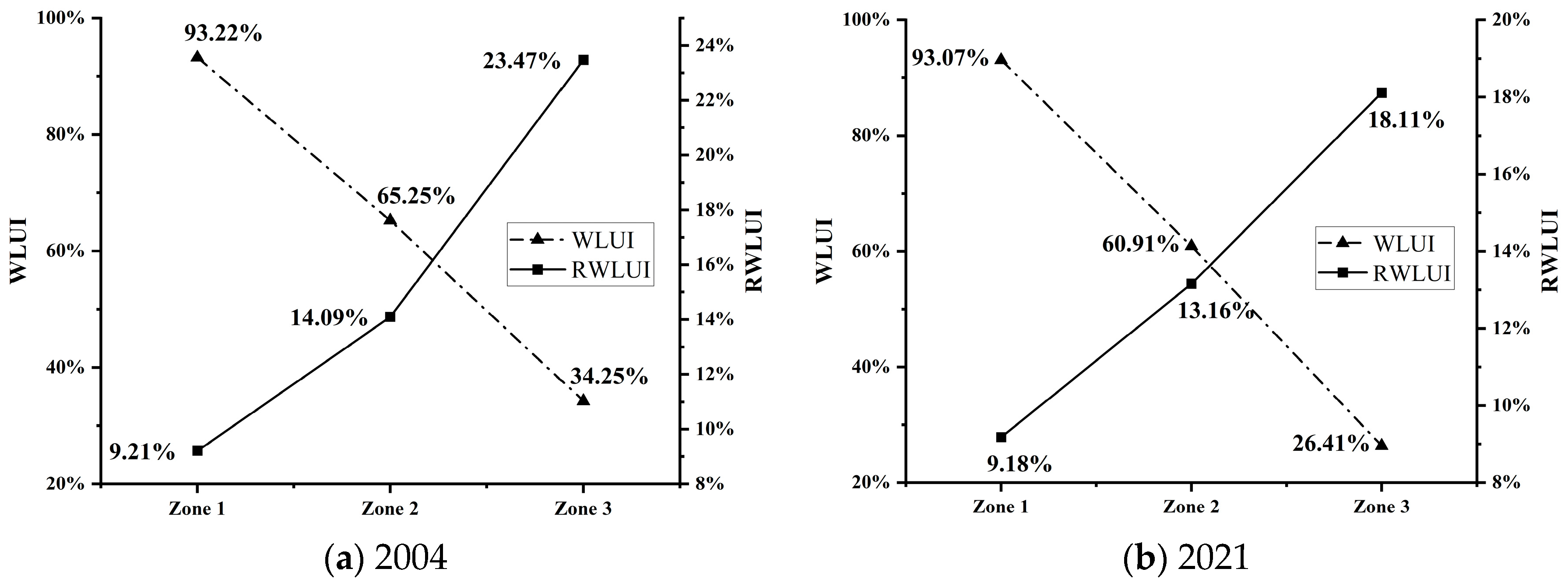
2.2.3. Calculation of Thermal Environment Contribution Based on Different Urban Zones

Urban development areas exhibit varying landscape patterns and LST, thus contributing different heat effects to the urban thermal environment [19]. It is necessary to further identify the influence of distinct urban zones on the urban thermal environment and analyze their variations across different dates. This analysis is invaluable for urban planners in determining how to mitigate the UHI effect through judicious landscape design and urban management.

In this study area, the entire region was divided into three concentric zones (Zone 1, Zone 2, and Zone 3) based on differing urban development densities, as shown in Figure 1. Differing from the thermal environment contribution index (CI_i) calculated by [41] for various land cover types, in this study, the CI_i, the weighted LST unit index (WLUI), and the regional weighted LST unit index (RWLUI) were employed to evaluate the heat contribution effects across different zones of the study area. The urban CI_i was calculated as follows:

$${\mathrm{C}\mathrm{I}}_{\mathrm{i}}={\displaystyle \frac{{\mathrm{C}\mathrm{I}}_{\mathrm{i}}^{\mathrm{*}}}{{\sum }_{\mathrm{i}=1}^{\mathrm{n}}{\mathrm{C}\mathrm{I}}_{\mathrm{i}}^{\mathrm{*}}}}\times 100\mathrm{\%}$$

(6)

$${\mathrm{C}\mathrm{I}}_{\mathrm{i}}^{\mathrm{*}}={\displaystyle \frac{\sum _{\mathrm{j}=1}^{{\mathrm{n}}_0}\left(\mathrm{L}\mathrm{S}{\mathrm{T}}_{\mathrm{i}\mathrm{j}}-{\mathrm{L}\mathrm{S}\mathrm{T}}_{\mathrm{m}\mathrm{e}\mathrm{a}\mathrm{n}}\right)\times {\mathrm{n}}_0}{{\mathrm{L}\mathrm{S}\mathrm{T}}_{\mathrm{m}\mathrm{e}\mathrm{a}\mathrm{n}}\times \mathrm{N}}}\times 100\mathrm{\%}$$

(7)

where ${\mathrm{C}\mathrm{I}}_{\mathrm{i}}^{\mathrm{*}}$ is the initial thermal environment contribution for the ith zone, LST_ij is the LST of the jth pixel in the ith zone with values that are larger than the mean LST of the whole study area (LST_mean), n₀ is the number of pixels with LST values larger than the value of LST_mean in the ith zone, and N is the number of pixels of the whole study area.

The WLUI describes the percentage of pixels with LST values larger than the LST_mean for the ith zone, whereas the RWLUI describes the percentage of the LST of the ith zone with values larger than the LST_mean of the whole study area. The two indices were calculated as follows:

$$\mathrm{W}\mathrm{L}\mathrm{U}\mathrm{I}={\displaystyle \frac{{\mathrm{n}}_{\mathrm{i}}}{{\mathrm{n}}_{\mathrm{z}\mathrm{o}\mathrm{n}\mathrm{e}\mathrm{i}}}}\times 100\mathrm{\%}$$

(8)

$$\mathrm{R}\mathrm{W}\mathrm{L}\mathrm{U}\mathrm{I}={\displaystyle \frac{{\mathrm{n}}_{\mathrm{i}}}{\mathrm{N}}}\times 100\mathrm{\%}$$

(9)

where n_zonei is the number of pixels for the ith zone, and i is 1, 2, or 3 in this study. N is also the number of pixels of the whole study area as in Equation (7).

In order to accurately describe the impacts of different landscape patterns on the urban thermal environment, it is necessary to calculate CI_i, WLUI, and RWLUI using Equations (6), (8) and (9) to further analyze the thermal environment impact of different urban development zones.

2.2.4. Spatial Statistical Analysis with Geographical Detector (Geodetector)

Spatial heterogeneity can reflect the spatial distribution of geographical phenomena and explain the former’s decisive factors and the latter’s interconnections [42,43]. The analysis of spatial heterogeneity can reveal the evolution of geographical features. In this study, the analysis of spatial heterogeneity was used to reveal the LST heterogeneity of urban expansion and its driving mechanisms.

Geodetector is a statistical tool used to quantitatively interpret geospatial heterogeneity and the driving forces of spatial differentiation. Through the constructed Geodetector model, the influence of different factors on geospatial phenomena and spatial differences can be calculated. This is measured by the q-statistic [42,44] as follows:

$$\begin{gathered} \mathrm{q}=1-{\displaystyle \frac{{\sum }_{\mathrm{H}=1}^{\mathrm{L}}{\mathrm{N}}_{\mathrm{h}}{\mathsf{\sigma }}_{\mathrm{h}}^2}{\mathrm{N}{\mathsf{\sigma }}^2}}=1-{\displaystyle \frac{\mathrm{S}\mathrm{S}\mathrm{W}}{\mathrm{S}\mathrm{S}\mathrm{T}}} \\ \mathrm{SSW}={\sum }_{\mathrm{H}=1}^{\mathrm{L}}{\mathrm{N}}_{\mathrm{h}}{\mathsf{\sigma }}_{\mathrm{h}}^2, \mathrm{SST}=\mathrm{N}{\mathsf{\sigma }}^2 \end{gathered}$$

(10)

where N_h and N are the number of samples in sub-region h (hth stratum) and the entire region, respectively; h = 1, 2, …; L is the stratification of impact factor X; σ² and σ_h² are the total variance of Y across the entire study area and the sub-region h, respectively. SSW and SST are the sum of the variance in each layer and the total variance of the region, respectively. The value of q ranges from 0 to 1; the larger the value, the greater the explanatory power or influence of X on the spatial differentiation of Y [45].

There are four detectors included in Geodetector, namely the factor detector, interaction detector, risk detector, and ecological detector. Risk detector and ecological detector are used to detect differences among the strata of a variable and between variables, respectively. The factor detector and interaction detector are applied in this study. The factor detector can explore and determine to what extent a factor X explains the spatial differentiation of Y. Factors that represent or control the spatial pattern of urban land use should play an important role in determining the spatial distribution of LST. In this study, we use the factor detector to detect the spatial heterogeneity of LST and identify the key driver factors behind the variation in LST. It is represented by q calculated as Equation (10); the q-value is used to measure the influence of each driving factor on LST. The greater the q-value, the greater the influence of the factor on LST, and the more obvious the influence on LST spatial differentiation. The interaction detector can distinguish and determine the interaction types between different factors X_i affecting Y, and evaluate whether the joint action of factors X₁ and X₂ (q(x₁ ∩ x₂)) will strengthen or weaken the explanatory power of dependent variable Y or whether their influences on Y are independent from each other.

Geodetector can be applied to identify the driving force behind elements by detecting their spatially layered heterogeneity [46]. In this study, the three different factors X_i are percent ISA, FVC, and elevation; the dependent variable Y is LST. Geodetector requires explanatory variables to be discretized; hence, each factor is pre-discretized into 5 intervals by the natural breakpoint method before analysis.

3. Results and Discussion

3.1. Analysis of the Spatial Pattern of LST in Different Urban Zones

In this study, the spatial pattern of LST and its variation were analyzed based on different zones between bi-temporal images. Figure 3c,d show that high LST (LST₄) and sub-high LST (LST₃) areas (areas with >LST_mean) were mainly distributed in the central zone (Zone 1) and some areas of Zone 2 in 2004. Zone 1 and part of Zone 2 were assembled with the ISA of buildings and roads, resulting in high and sub-high LST areas in both years. Meanwhile, the distribution of LST₄ and LST₃ areas in Zone 2 and Zone 3 in 2021 was notably larger than in 2004. In Zone 2 and Zone 3, the extent of the spatial distribution of LST₄ and LST₃ areas significantly increased from 2004 to 2021, especially in Zone 2 and the western part of Zone 3. This indicates that urban expansion resulted in an increase in LST, primarily in Zone 2 and Zone 3 between the two years.

The medium (LST₂) and low (LST₁) LST areas were mainly distributed in Zone 2 and Zone 3 of peri-urban areas in both images, especially Zone 3. This was limited by terrain and topography because LST₂ and LST₁ areas were characterized by forested and water-covered regions in mountainous areas. Urban expansion led to a transformation in land cover from natural to ISA, mainly occurring in the south and west plain areas of Zone 2 and Zone 3 from 2004 to 2021. The land cover types in the northern areas of Zone 2 and Zone 3 changed little from 2004 to 2021 due to mountainous constraints; consequently, the medium and low LST areas experienced minimal change in these regions during the period.

To further quantify the impact of high and sub-high LST areas on the thermal environment, we need to analyze the change in the areal proportion of high and sub-high LST areas with urban expansion.

Table 2. The areal proportion of high and sub-high LST categories in each zone and the whole high and sub-high LST area of the study area.

	Areal Proportion of LST3 and LST4 in Each Zone		Areal Proportion of LST3 and LST4 in Each Zone to Whole LST3 and LST4 Area of the Study Area
	2004	2021	2004	2021
Zone 1	94.99%	92.98%	26.58%	20.78%
Zone 2	56.11%	62.03%	34.97%	31.04%
Zone 3	21.08%	32.49%	38.45%	48.18%

shows the areal proportions of the LST₄ and LST₃ categories in each zone and the total LST₄ and LST₃ area of the study area. As shown in Figure 3, LST₄ and LST₃ areas dominated Zone 1, accounting for 94.99% in 2004. However, the areal proportions of LST₄ and LST₃ areas in Zone 1 decreased slightly to 92.98% in 2021, likely due to increased attention to urban ecology; consequently, greater vegetation cover was interspersed in some areas of Zone 1 after 2004. For Zone 2 and Zone 3, the areal proportions of LST₄ and LST₃ areas increased from 56.11% and 21.08% to 62.03% and 32.49%, respectively, from 2004 to 2021. This indicates that the high and sub-high LST areas exceeded LST_mean in this study area, primarily resulting from urban expansion in Zone 2 and Zone 3 during this period.

As for the areal proportions of high and sub-high LST areas in each zone relative to the total high and sub-high LST areas of the entire study area, the areal proportions of LST₄ and LST₃ areas in Zone 1 decreased from 26.58% to 20.78% during the period. In Zone 2, areal proportions also decreased from 34.97% to 31.04%. However, the areal proportions of LST₄ and LST₃ areas in Zone 3 relative to those of the entire study area increased from 38.45% to 48.18% in the same period. This indicates that, with urban expansion, high and sub-high LST areas mainly increased in Zone 3, followed by Zone 2. Although the area of high and sub-high LST also increased in Zone 2, as shown in Figure 3, the rate of increase was slower compared to that of Zone 3 when considering the entire study area (Table 2).

Obviously, Zone 1 had the highest LST in general, followed by Zone 2 and then Zone 3. The high and sub-high-level LST areas were heat sources contributing to the UHI effect. The lowest LST areas are primarily vegetation areas, which act as heat sinks. Although Zone 2 has a cooling thermal environment due to its vegetation area, its cooling effect is limited due to the small area of vegetation. In Zone 3, there are numerous vegetation areas that serve as major heat sinks, playing the most significant role in cooling the thermal environment in the study area. Additionally, the lowest LST areas also occur in the water bodies of all three zones.

3.2. Analysis of Thermal Environment Contribution in Each Urban Zone

Quantitative analysis of the thermal environmental impacts of different urban landscape patterns becomes important in urban ecology because of urban thermal environment problems. In this study, Zone 1 obviously shows a higher LST, followed by Zone 2 and Zone 3. However, the heat effects of each zone on the thermal environment and their changes between different dates require further analysis. In order to further quantify the heat contribution in detail, Equation (6) was used to calculate the CI_i and to further analyze the thermal environmental impact of different zones in this study (Figure 5).

Urban expansion with ISA clearly resulted in an increase in LST. As shown in Figure 5, the CI_i of Zone 1 and Zone 2 were 24.84% and 33.44% in 2004, respectively. With the urban expansion resulting in LST variation, the CI_i of Zone 1 and Zone 2 decreased to 10.61% and 25.91% in 2021, respectively. However, the CI_i of Zone 3 increased from 41.72% in 2004 to 63.49% in 2021. Though ISA increased in Zone 2 and Zone 3 in the study area, and the area of ISA with >LST_mean also increased in Zone 2 from 2004 to 2021 (Table 2), the increase rate of ISA with >LST_mean was higher in Zone 3 than in Zone 2 in the period. This resulted in a decrease in CI_i in Zone 2. Figure 5 indicates that urban expansion, coupled with areas exhibiting >LST_mean, has led to thermal environment issues, predominantly escalating in Zones 2 and 3 during this period, particularly in Zone 3. Zones 3 and 2 exhibited relatively high CI_i values in the two years compared to Zone 1, with Zone 3 being the primary source of the heat effect in the study area and Zone 2 in second place. Although the CI_i values of Zone 1 obviously decreased, the area with >LST_mean decreased only slightly between the two dates (Table 2). The increase in ISA with >LST_mean was more pronounced in Zone 3 and Zone 2 than in Zone 1 from 2004 to 2021.

Compared with Zone 1, the CI_i values of Zone 2 decreased relatively little between the two dates. From 2004 to 2021, the CI_i of Zone 3 increased significantly and contributed 63.49% of the heat effect in the entire study area in 2021, whereas the influence of Zone 3 on the thermal environment was not significant in 2004. The thermal environment impact of Zone 3 increased significantly in 2021 due to urban expansion. The CI_i of Zones 2 and 3 reached from 75.16% in 2004 to 89.40% in 2021, indicating that the heat effect contribution was determined and dominated by Zones 2 and 3 in the study area.

The different urban development zones exhibited distinct landscape patterns and LST features. To further quantify the impact and pattern of the thermal environment, WLUI and RWLUI were calculated based on Equations (8) and (9) to assess the thermal contribution effects of different zones in the study area (Figure 6). WLUI represents the percentage of pixels with values exceeding the LST_mean for each zone. Figure 6 showed that the WLUI of Zone 1 was high, accounting for approximately 93.07% and 93.22% from 2004 to 2021, with little change between the two dates. The WLUI of Zone 1 indicated that areas with high and sub-high LST (>LST_mean area) dominated in Zone 1, with the areal ratio reaching over 93% in the urban core zone with high development density. Meanwhile, the WLUI values for Zone 2 and Zone 3, respectively, decreased in sequence from Zone 1 to Zone 3 on both dates. Comparing WLUI values on both dates, WLUI values in Zone 2 and Zone 3 increased from 60.91% and 26.41% in 2004 to 65.25% and 34.25% in 2021, respectively. This reflects a higher rate of increase in WLUI in Zone 3 compared to Zone 2, indicating an amplified thermal environment impact in both zones from 2004 to 2021. The WLUI values of Zone 2 and Zone 3 indicate that >LST_mean areas increased in areas of medium development density and low development density with expansion in the period.

The RWLUI is the percentage of the high and sub-high LST area of each zone relative to the whole study area (Figure 6). The RWLUI values of Zone 1 were 9.18% in 2004 and 9.21% in 2021. From the perspective of the whole study area, the thermal environment impact of Zone 1 did not significantly strengthen from 2004 to 2021 because urban expansion mainly occurred in Zones 2 and 3 during this period. The RWLUI values for Zone 2 and Zone 3 continued to increase from 13.16% and 18.11% in 2004 to 14.09% and 23.47% in 2021, respectively.

The increase in thermal environment contribution indicates that high and sub-high LST areas increased with the rise in high percent ISA resulting from urban expansion. Figure 5 and Figure 6 indicated that, though the areal proportion of high and sub-high LST areas was dominant in Zone 1 and the lowest in Zone 3, the contribution of Zone 3 to regional heat in the study area was higher than those of Zone 2 and Zone 1. This is because Zone 3 contributes the most high and sub-high LST area among the three zones, followed by Zone 2 and Zone 1. Our analysis revealed the characteristics of the thermal environment effects and their variation in different development density areas at two different time points. By analyzing CI_i, WLUI, and RWLUI of each zone and their variations, we can quantify the thermal environmental contribution of different development density areas with urban expansion. Different from other analyses of thermal environmental contribution based on different land cover types, this analysis is significant for urban planning, UHI mitigation, and urban ecology.

3.3. Driving Force Detection of Spatial Heterogeneity of LST by Geodetector

The spatial distribution and aggregation of LST were different in different urban development areas. The spatial distribution pattern of LST is related to the degree of urban expansion and is impacted by different land cover types, the combination and configuration of various land cover types, and other factors. Detection of driving forces behind urban LST heterogeneity is crucial for alleviating UHI and adapting to urban climatic change. The spatial heterogeneity of LST results from the spatial distribution of different land cover types and other factors [47]. In this study, percent ISA, fractional vegetation cover, and elevation were selected as independent variables (X) and were all categorized into five types based on the Jenks natural breaks classification method. LST was selected as the dependent variable (Y). The influences of X on the spatial differentiation of Y in different zones in 2004 and 2021 were calculated using Geodetector and further comparatively analyzed.

In this study, the factor differentiation detector was used to reveal the impact of each factor on the spatial distribution of LST.

Table 3. The q-values of the factors influencing LST heterogeneity in different zones of the study area in 2004 and 2021.

Single Factor	Q in Zone1		Q in Zone 2		Q in Zone 3
	2004	2021	2004	2021	2004	2021
Percent ISA	0.134	0.186	0.349	0.527	0.224	0.543
FVC	0.309	0.144	0.581	0.572	0.494	0.602
Elevation	0.203	0.115	0.558	0.653	0.432	0.681

p < 0.01, the significance of the q-value was determined using an F test with a significance level of 0.01.

shows the q-values of three single factors on the spatial distribution of LST, and all were significant (p < 0.01). In the study area, the degree of influence of the three driving factors on the spatial distribution of LST varied in different development densities of the urban area. The q-values of three influencing factors in Zone 1 were relatively low (≤0.309) on both dates, and variations were also small in Zone 1 between the two dates (Table 3). This indicates that the urban landscape pattern changes and urban expansion nearly did not exist in the urban core Zone 1 from 2004 to 2021. Among the influencing factors, the FVC had a greater impact on LST in Zone 1 in 2004. From 2004 to 2021, the q-value of FVC decreased from 0.309 to 0.144 in Zone 1. According to the principles of Geodetector, the larger the q-value, the greater the driving force of the factor on LST. Table 3 indicates that the three factors had a lesser degree of influence on the heterogeneity of LST, and the spatial distribution patterns of LST varied minimally in Zone 1 between the two dates.

The three factors had a greater influence in Zone 2 and Zone 3 than in Zone 1 on both dates. When comparing the q-values of the three influencing factors between the two dates, the q-values in Zone 2 and Zone 3 in 2021 were larger than those in 2004, except for the q-value of FVC in Zone 2 in 2004, which was slightly larger than that of Zone 2 in 2021. The results from the factor detection analysis showed that the largest q-values were 0.581 and 0.653 in Zone 2 in 2014 and 2021, respectively, and 0.494 and 0.681 in Zone 3 in 2004 and 2021, respectively. This indicated that FVC had the most significant influence on LST heterogeneity in Zone 2 and Zone 3 in 2004, while elevation had the greatest influence on LST heterogeneity in Zone 2 and Zone 3 in 2021. This is because the landscape pattern changes due to urban expansion were influenced by topography (elevation) in Zone 3 in 2021, which had a certain impact on the q-value of Zone 3. The elevation was ranked next, with values of 0.558 and 0.432 in Zone 2 and Zone 3 in 2004, respectively, and FVC was ranked next to elevation, with values of 0.572 and 0.602 in Zone 2 and Zone 3 in 2021, respectively.

When comparing the q-values between Zone 2 and Zone 3, the q-values of the three influencing factors were smaller in Zone 3 than in Zone 2 in 2004. However, the q-values of the three influencing factors were larger in Zone 3 than in Zone 2 in 2021. This is related to the change in urban landscape patterns in Zone 2 and Zone 3 resulting from urban expansion. FVC and elevation had a higher influence degree than percent ISA in Zone 2 and Zone 3 in 2004. The explanatory power (q-value × 100%) of FVC and elevation decreased from 58.1% and 55.8% in Zone 2 to 49.4% and 43.2% in Zone 3, respectively, in 2004, and increased from Zone 2 to Zone 3 in 2021. This indicates that urban expansion also resulted in the change in landscape patterns in some higher-elevation areas of Zone 3. FVC and elevation had a higher influence degree on the spatial heterogeneity of LST in Zone 2 and Zone 3 in both years. However, the explanatory power of percent ISA significantly increased from 34.9% to 52.7% in Zone 2 and from 22.4% to 54.3% in Zone 3 from 2004 to 2021. Though the q-values of FVC and elevation in Zone 2 and Zone 3 were larger than that of percent ISA in 2004, the q-values of the influencing factor percent ISA significantly increased from 2004 to 2021 with urban expansion.

According to the above analysis, the three factors have weak explanatory power for the spatial heterogeneity of LST in Zone 1 compared to Zone 2 and Zone 3. This means that the changes in landscape patterns resulting from urban expansion significantly increased the degree of influence of the three driving factors on LST in Zone 2 and Zone 3 compared to Zone 1. In different urban development areas, the land cover types and their spatial distribution are different, which influences the value and spatial distribution of LST. In Zone 1 of the urban core area, a high percent ISA is distributed homogeneously, resulting in the homogeneity of the spatial distribution of high LST. Therefore, the influence degree of the three factors on LST heterogeneity is low. However, in Zone 3 and Zone 2, the three factors have a higher influence degree on the spatial distribution of LST. This indicates that they are the main driving factors affecting the LST in Zone 2 and Zone 3, especially the elevation factor in Zone 3 in 2021. However, no one single factor dominantly affects LST distribution in Zone 2 and Zone 3 of the study area. Through analyzing and comparing the q-values of different zones, we can understand the driving force of LST distribution in different development areas, which will help in constructing a good urban ecological environment.

The spatial distribution of urban landscapes and thermal patterns is usually the result of multifactor interactions. The influence of the interaction between different factors may be stronger than that of a single factor when each factor interacts with others on LST. Therefore, it is necessary to analyze the influence of the interaction between any two factors on the spatial difference in LST. Through interactive calculation of different driving factors in Geodetector, we analyzed the interactive detection of various driving factors on LST distribution for both years. The q-value is defined as q (X₁ ∩ X₂), and the results are shown in

Table 4. The q-values of interactive detection of driving factors on LST in different zones of the study area in 2004 and 2021 (EL is elevation).

Interactive Factors	q in Zone1		q in Zone 2		q in Zone 3
	2004	2021	2004	2021	2004	2021
percent ISA ∩ FVC	0.332	0.202	0.596	0.591	0.510	0.616
percent ISA ∩ EL	0.279	0.261	0.637	0.749	0.489	0.757
FVC ∩ EL	0.375	0.228	0.743	0.558	0.621	0.767

All were nonlinear enhancement; p < 0.01, the significance of the q-value was determined using an F-test with a significance level of 0.01.

. Compared with the results of single-factor detection in Table 3, Table 4 shows that the q-value increases significantly when each driving factor interacts with other factors, and its influence on LST increases, indicating that LST is a geographical pattern driven by multi-factor interaction.

The interaction detector creates a new stratum by overlaying factors X₁ and X₂ to further compare q(X₁ ∩ X₂) with q(X₁) and q(X₂) [48]. The results of interaction detection can show whether the combined effects of the evaluation indicators X₁ and X₂ enhance, bi-enhance, nonlinearly enhance, weaken, bi-weaken, or nonlinearly weaken the explanatory power of LST heterogeneity or whether the combined effects on LST are independent of each other. In this study, the explanatory power of the interactions of different factors in Table 4 was larger than that of the single factor in Table 3, and all the interactive factors showed nonlinear enhancement in 2004 and 2021. This indicates that the interaction between any two factors of percent ISA, FVC, and elevation amplifies their impact on LST distribution in the three zones during both years. The q-values of interaction detection were significantly larger than those of single-factor detection in Table 3 in both years. This means that interactions between different factors have higher explanatory power on the LST heterogeneity in each zone than single factors alone. The results from interaction detection analysis showed that the q-values of interactions of three factors at Zone 1 were lower than those of Zone 2 and Zone 3 (Table 4). This trend is the same as that in Table 3. This is because the landscape patterns of Zone 1 are significantly different from those in Zone 2 and Zone 3. Though the q-values of interactions of three factors increased in Zone 1 in both years, the q-values of interactions of three factors also significantly increased in Zones 2 and 3 in both years when compared with those of the single factor in Table 3.

As shown in Table 4, the results from interaction detection analysis showed that FVC ∩ EL and percent ISA ∩ EL in Zone 2 were 0.743 and 0.749 (74.3% and 74.9% explanatory power on the LST heterogeneity) in 2004 and 2021, respectively, and were the most significant influences on LST heterogeneity in Zone 2. The interactions of percent ISA ∩ EL and percent ISA ∩ FVC were ranked next in Zone 2 in 2004 and 2021, with values of 0.637 and 0.591 in 2004 and 2021, respectively. As for Zone 3, FVC ∩ EL was the most significant influence on LST heterogeneity in both years; the q-value was 0.621 and 0.767 in 2004 and 2021, respectively. Percent ISA ∩ FVC with a value of 0.510 and percent ISA ∩ EL with a value of 0.757 were ranked next in Zone 3 in 2004 and 2021, respectively. Based on the analysis of the interaction between two factors, we can determine which kind of interaction has the strongest influence on the spatial heterogeneity of LST. This can help guide the composition and configuration of driving factors in different urban development areas for UHI.

In the study area, it was found that the influencing factors differed across the three zones. Synthetically evaluating the results of factor and interaction detection, it is worth noting that the landscape pattern of urban expansion in Zone 3 was limited by geomorphologic characterization, and elevation leads to an imbalanced distribution of LST in Zone 3. When urban expansion was intense in Zone 3, it was clear that most of the new urban area was distributed around the mountain. This led to an imbalance in urban expansion and also had a certain impact on the q-value of Zone 3. In addition, as a single factor, FVC had a high influence on LST heterogeneity in Zones 2 and 3 of the study area.

Linear correlation cannot analyze the consistency of spatial distribution between two geographic variables. Compared with linear correlation analysis, Geodetector can reveal the causal relationship between independent and dependent variables [48]. In this study, Geodetector was used to show the driving force of different factors on the heterogeneity of LST resulting from urban landscape expansion through the q-value. The spatial heterogeneity of LST may come from an imbalance in urban expansion. This analysis can reveal this imbalance and further help to understand the influencing factors of LST in different urban development areas. It can provide significant information for urban planning and coping with urban climatic change.

4. Conclusions

Urban expansion changes the urban landscape pattern and also the spatial distribution of LST, and may have an effect on human health. This study aimed to explore the impact of urban expansion on the thermal environment in different development density areas. Bi-temporal Landsat images were used to derive LST, percent ISA, and FVC, and CI_i, WLUI, and RWLUI were further calculated to analyze the thermal environment contribution based on different urban zones. Geodetector was also used to explore the driving factors controlling the spatial heterogeneities of LST. This study compared the CI_i, WLUI, RWLUI_, and q between different urban zones and different dates by revealing the thermal contribution of different urban landscape patterns and the factors controlling spatial heterogeneities of LST in different urban development areas. Though the research is focused only on one city, the analytical method can provide insights for quantifying urban landscape patterns and thermal environments in other cities. This could help alleviate the negative effects of urbanization and provide a reference for urban landscape design in other cities with different development areas. The results of the study can help mitigate the UHI effect and adapt to climatic change in cities. In this study, four conclusions were as follows:

(1)

ISA increase resulting from urban expansion mainly concentrated in the south and west areas of Zones 2 and 3 from 2004 to 2021, and the high and sub-high LST areas also mainly increased in Zone 2 and Zone 3 during the period.

(2)

The thermal environment contribution of Zone 3 significantly increased from 2004 to 2021. The CI_i of Zones 2 and 3 reached over 89% in 2021, and the thermal environment contribution was determined and dominated by Zone 2 and Zone 3 in the study area in 2021.

(3)

In the study area, the driving factors affecting the spatial differentiation of LST are regionally different, and the influence degree of three factors on LST is weaker in Zone 1 than in Zones 2 and 3. Compared with a single factor, the interaction between different factors can increase the influence on LST.

(4)

The combined analysis of thermal environment contribution and Geodetector provides a suitable method to reveal the impact of the urban landscape pattern on the urban thermal environment and the driving mechanisms of LST heterogeneity. The analytic results can provide a deeper understanding of the mechanisms of the UHI and provide recommendations for mitigating UHI.

In this study, Landsat images from the summer were used to reveal thermal contribution and heterogeneous analysis of LST; all four seasons should be considered in future analysis. In addition, we believe that the spatial scale of environmental factors is important in affecting LST, and heat contribution and LST heterogeneity may be different at different spatial scales. Therefore, multi-scale heat contributions, environmental factors, and LST should be taken into account in further comparative analysis in the future.

References

1. Huang, X.; Wang, Y. Investigating the effects of 3D urban morphology on the surface urban heat island effect in urban functional zones by using high-resolution remote sensing data: A case study of Wuhan, Central China. ISPRS J. Photogramm. Remote Sens. 2019, 152, 119–131. [Google Scholar] [CrossRef]
2. Zhang, Y.; Wang, X.; Balzter, H.; Qiu, B.; Cheng, J. Directional and Zonal Analysis of Urban Thermal Environmental Change in Fuzhou as an Indicator of Urban Landscape Transformation. Remote Sens. 2019, 11, 2810. [Google Scholar] [CrossRef]
3. Hu, X.; Xu, H. A new remote sensing index for assessing the spatial heterogeneity in urban ecological quality: A case from Fuzhou City, China. Ecol. Indic. 2018, 89, 11–21. [Google Scholar] [CrossRef]
4. Oke, T. Street design and urban canopy layer climate. Energy Build. 1988, 11, 103–113. [Google Scholar] [CrossRef]
5. Parker, D.E. Urban heat island effects on estimates of observed climate change. Wiley Interdiscip. Rev. Clim. Chang. 2010, 1, 123–133. [Google Scholar] [CrossRef]
6. Zhou, W.; Qian, Y.; Li, X.; Li, W.; Han, L. Relationships between land cover and the surface urban heat island: Seasonal variability and effects of spatial and thematic resolution of land cover data on predicting land surface temperatures. Landsc. Ecol. 2014, 29, 153–167. [Google Scholar] [CrossRef]
7. Zhou, W.; Wang, J.; Cadenasso, M. Effects of the spatial configuration of trees on urban heat mitigation: A comparative study. Remote Sens. Environ. 2017, 195, 1–12. [Google Scholar] [CrossRef]
8. Zhang, Y.; Odeh, I.; Han, C. Bi-temporal characterization of land surface temperature in relation to impervious surface area, NDVI and NDBI, using a sub-pixel image analysis. Int. J. Appl. Earth Obs. Geoinf. 2009, 11, 256–264. [Google Scholar] [CrossRef]
9. Frazier, A.E.; Wang, L. Characterizing spatial patterns of invasive species using sub-pixel classifications. Remote Sens. Environ. 2011, 115, 1997–2007. [Google Scholar] [CrossRef]
10. Du, J.; Xiang, X.; Zhao, B.; Zhou, H. Impact of urban expansion on land surface temperature in Fuzhou, China using Landsat imagery. Sustain. Cities Soc. 2020, 61, 102346. [Google Scholar] [CrossRef]
11. Lu, D.; Weng, Q. Use of impervious surface in urban land-use classification. Remote Sens. Environ. 2006, 102, 146–160. [Google Scholar] [CrossRef]
12. Owen, T.; Carlson, T.; Gillies, R. An assessment of satellite remotely sensed land cover parameters in quantitatively describing the climatic effect of urbanization. Int. J. Remote Sens. 1998, 19, 1663–1681. [Google Scholar] [CrossRef]
13. Chen, X.; Zhao, M.; Li, P.; Yin, Z. Remote sensing image based analysis of the relationship between urban heat island and land use/cover changes. Remote Sens. Environ. 2006, 104, 133–146. [Google Scholar] [CrossRef]
14. Alexander, C. Influence of the proportion, height and proximity of vegetation and buildings on urban land surface temperature. Int. J. Appl. Earth Obs. Geoinf. 2021, 95, 102265. [Google Scholar] [CrossRef]
15. Zhang, Y.; Balzter, H.; Li, Y. Influence of Impervious Surface Area and Fractional Vegetation Cover on Seasonal Urban Surface Heating/Cooling Rates. Remote Sens. 2021, 13, 1263. [Google Scholar] [CrossRef]
16. Cao, X.; Onishi, A.; Chen, J.; Imura, H. Quantifying the cool island intensity of urban parks using ASTER and IKONOS data. Landsc. Urban. Plan. 2010, 96, 224–231. [Google Scholar] [CrossRef]
17. Klok, L.; Zwart, S.; Verhagen, H.; Mauri, E. The surface heat island of Rotterdam and its relationship with urban surface characteristics. Res. Conserv. Recycl. 2012, 64, 23–29. [Google Scholar] [CrossRef]
18. Deng, C.; Wu, C. Estimating very high resolution urban surface temperature using a spectral unmixing and thermal mixing approach. Int. J. Appl. Earth Obs. Geoinf. 2013, 23, 155–164. [Google Scholar] [CrossRef]
19. Berger, C.; Rosentreter, J.; Voltersen, M.; Baumgart, C.; Schmullius, C.; Hese, S. Spatio-temporal analysis of the relationship between 2D/3D urban site characteristics and land surface temperature. Remote Sens. Environ. 2017, 193, 225–243. [Google Scholar] [CrossRef]
20. Zhang, Y.; Harris, A.; Balzter, H. Characterizing fractional vegetation cover and land surface temperature based on sub-pixel fractional impervious surfaces from Landsat TM/ETM+. Int. J. Remote Sens. 2015, 36, 4213–4232. [Google Scholar] [CrossRef]
21. Zhang, Y.; Balzter, H.; Liu, B.; Chen, Y. Analyzing the Impacts of Urbanization and Seasonal Variation on Land Surface Temperature Based on Subpixel Fractional Covers Using Landsat Images. IEEE J. Sel. Top. Appl. Earth Obs. Remote Sens. 2017, 10, 1344–1356. [Google Scholar] [CrossRef]
22. He, C.; Gao, B.; Huang, Q.; Ma, Q.; Dou, Y. Environmental degradation in the urban areas of China: Evidence from multi-source remote sensing data. Remote Sens. Environ. 2017, 193, 65–75. [Google Scholar] [CrossRef]
23. Shen, H.; Huang, L.; Zhang, L.; Wu, P.; Zeng, C. Long-term and fine-scale satellite monitoring of the urban heat island effect by the fusion of multi-temporal and multi-sensor remote sensed data: A 26-year case study of the city of Wuhan in China. Remote Sens. Environ. 2016, 172, 109–125. [Google Scholar] [CrossRef]
24. Peng, W.; Yuan, X.; Gao, W.; Wang, R.; Chen, W. Assessment of urban cooling effect based on downscaled land surface temperature: A case study for Fukuoka, Japan. Urban Clim. 2021, 36, 100790. [Google Scholar] [CrossRef]
25. Han, S.; Hou, H.; Estoque, R.; Zhang, Y.; Shen, C.; Murayama, Y.; Pan, J.; Wang, B.; Hu, T. Seasonal effects of urban morphology on land surface temperature in a three-dimensional perspective: A case study in Hangzhou, China. Build. Environ. 2023, 228, 109913. [Google Scholar] [CrossRef]
26. Guo, G.; Zhou, X.; Wu, Z.; Xiao, R.; Chen, Y. Characterizing the impact of urban morphology heterogeneity on land surface temperature in Guangzhou, China. Environ. Model. Softw. 2016, 84, 427–439. [Google Scholar] [CrossRef]
27. Song, J.; Chen, W.; Zhang, J.; Huang, K.; Hou, B.; Prishchepov, A. Effects of building density on land surface temperature in China: Spatial patterns and determinants. Landsc. Urban. Plan. 2020, 198, 103794. [Google Scholar] [CrossRef]
28. Boori, M.; Choudhary, K.; Paringer, R.; Kupriyanov, A. Spatiotemporal ecological vulnerability analysis with statistical correlation based on satellite remote sensing in Samara, Russia. J. Environ. Manag. 2021, 285, 112138. [Google Scholar] [CrossRef] [PubMed]
29. Guo, L.; Liu, R.; Men, C.; Wang, Q.; Miao, Y.; Zhang, Y. Quantifying and simulating landscape composition and pattern impacts on land surface temperature: A decadal study of the rapidly urbanizing city of Beijing, China. Sci. Total Environ. 2019, 654, 430–440. [Google Scholar] [CrossRef] [PubMed]
30. Liu, J.; Xu, Q.; Yi, J.; Huang, X. Analysis of the heterogeneity of urban expansion landscape patterns and driving factors based on a combined Multi-Order Adjacency Index and Geodetector model. Ecol. Indic. 2022, 136, 108655. [Google Scholar] [CrossRef]
31. Li, X.; Li, W.; Middel, A.; Harlan, S.L.; Brazel, A.J.; Turner, B.L. Remote sensing of the surface urban heat island and land architecture in Phoenix, Arizona: Combined effects of land composition and configuration and cadastral–demographic–economic factors. Remote Sens. Environ. 2016, 174, 233–243. [Google Scholar] [CrossRef]
32. Omurakunova, G.; Bao, A.; Xu, W.; Duulatov, E.; Jiang, L.; Cai, P.; Abdullaev, F.; Nzabarinda, V.; Durdiev, K.; Baiseitova, M. Expansion of Impervious Surfaces and Their Driving Forces in Highly Urbanized Cities in Kyrgyzstan. Int. J. Environ. Res. Public Health 2020, 17, 362. [Google Scholar] [CrossRef] [PubMed]
33. Wang, J.; Ouyang, W. Attenuating the surface urban heat island within the local thermal zones through land surface modification. J. Environ. Manag. 2017, 187, 239–252. [Google Scholar] [CrossRef] [PubMed]
34. Shi, T.; Hu, Z.; Shi, Z.; Guo, L.; Chen, Y.; Li, Q.; Wu, G. Geo-detection of factors controlling spatial patterns of heavy metals in urban topsoil using multi-source data. Sci. Total Environ. 2018, 643, 451–459. [Google Scholar] [CrossRef] [PubMed]
35. Voogt, J.A.; Oke, T.R. Thermal remote sensing of urban climates. Remote Sens. Environ. 2003, 86, 370–384. [Google Scholar] [CrossRef]
36. Barsi, J.; Schott, J.; Palluconi, F.; Hook, S. Validation of a web-based atmospheric correction tool for single thermal band instruments. In Earth Observing Systems X; Butler, J.J., Ed.; Paper 58820E; SPIE: Bellingham, WA, USA, 2005; Volume 5882. [Google Scholar]
37. Sobrino, J.; Raissouni, N.; Li, Z. A comparative study of land surface emissivity retrieval from NOAA data. Remote Sens. Environ. 2001, 75, 256–266. [Google Scholar] [CrossRef]
38. Van De Grienzd, A.; Owe, M. On the relationship between thermal emissivity and the normalized difference vegetation index for natural surfaces. Int. J. Remote Sens. 1993, 14, 1119–1131. [Google Scholar] [CrossRef]
39. Chander, G.; Markham, B. Revised Landsat-5 TM radiometric calibration procedures and post calibration dynamic ranges. IEEE Trans. Geosci. Remote Sens. 2003, 41, 2674–2677. [Google Scholar] [CrossRef]
40. Mitraka, Z.; Chrysoulakis, N.; Kamarianakis, Y.; Partsinevelos, P.; Tsouchlaraki, A. Improving the estimation of urban surface emissivity based on sub-pixel classification of high resolution satellite imagery. Remote Sens. Environ. 2012, 117, 125–134. [Google Scholar] [CrossRef]
41. Liu, Y.; Kuang, Y.Q.; Wu, Z.F.; Huang, N.S.; Zhou, J. Impact of land use on urban land surface temperature: A case study of Dongguan, Guangdong Province. J. Geogr. Sci. 2006, 26, 597–602. [Google Scholar]
42. Wang, J.; Zhang, T.; Fu, B. A measure of spatial stratified heterogeneity. Ecol. Indicat. 2016, 67, 250–256. [Google Scholar] [CrossRef]
43. Shen, Z.; Zhang, W.; Peng, H.; Xu, G.; Chen, X.; Zhang, X.; Zhao, Y. Spatial characteristics of nutrient budget on town scale in the Three Gorges Reservoir area, China. Sci. Total Environ. 2022, 819, 152677. [Google Scholar] [CrossRef] [PubMed]
44. Song, Y.; Wang, J.; Ge, Y.; Xu, C. An optimal parameters-based geographical detector model enhances geographic characteristics of explanatory variables for spatial heterogeneity analysis: Cases with different types of spatial data. Gisci. Rem. Sens. 2020, 57, 593–610. [Google Scholar] [CrossRef]
45. Zhu, X.; Yang, Y.; Li, X.; Zhang, X.; Shan, L. Research on landsat 8 surface temperature inversion algorithm. Geospatial. Inform. 2018, 16, 103–106. [Google Scholar]
46. Wang, J.; Li, X.; Christakos, G.; Liao, Y.L.; Zhang, T.; Gu, X.; Zheng, X.Y. Geographical detectors-based health risk assessment and its application in the neural tube defects study of the Heshun region, China. Int. J. Geogr. Inf. Sci. 2010, 24, 107–127. [Google Scholar] [CrossRef]
47. Guo, B.; Wei, C.; Yu, Y.; Liu, Y.; Li, J.; Meng, C.; Cai, Y. The dominant influencing factors of desertification changes in the source region of Yellow River: Climate change or human activity? Sci. Total Environ. 2022, 813, 152512. [Google Scholar] [CrossRef] [PubMed]
48. Wang, J.; Xu, C. Geodetector: Principle and prospective. Acta. Geogr. Sin. 2017, 72, 116–134. [Google Scholar]
Figure 1. The location and Landsat 8 image acquired on 27 September 2021 (a false-color composite image: red, band 5; green, band 4; blue, band 3) of the study area. (The study area was divided into three sectors from the city center to urban peripheral areas in the right figure. The five sample plots delineated with polygons, representing test sites, were used for accuracy assessment in Table 1).
Remotesensing 16 02973 g001
Figure 2. Flowchart showing the steps in the study.
Remotesensing 16 02973 g002
Figure 3. Spatial distribution patterns of LST and LST classification: (a) Spatial distribution patterns of LST in 2004. (b) Spatial distribution patterns of LST in 2021. (c) Four LST classes in 2004. (d) Four LST classes in 2021.
Remotesensing 16 02973 g003
Figure 4. Fractional ISA and FVC derived from ETM+/OLI images using FCLS: (a) 2004 fractional ISA, (b) 2004 FVC, (c) 2021 fractional ISA, and (d) 2021 FVC.
Remotesensing 16 02973 g004aRemotesensing 16 02973 g004b
Figure 5. Thermal environment contribution index of each zone to the whole study area of Fuzhou.
Remotesensing 16 02973 g005
Figure 6. Thermal environment effect of each zone (WLUI and RWLUI) in the study area of Fuzhou in (a) 2004 and (b) 2021.
Remotesensing 16 02973 g006