A Feature Line Extraction Method for Building Roof Point Clouds Considering the Grid Center of Gravity Distribution

Abstract

Feature line extraction for building roofs is a critical step in the 3D model reconstruction of buildings. A feature line extraction algorithm for building roof point clouds based on the linear distribution characteristics of neighborhood points was proposed in this study. First, the virtual grid was utilized to provide local neighborhood information for the point clouds, aiding in identifying the linear distribution characteristics of the center of the gravity points on the feature line and determining the potential feature point set in the original point clouds. Next, initial segment elements were selected from the feature point set, and the iterative growth of these initial segment elements was performed by combining the RANSAC linear fitting algorithm with the distance constraint. Compatibility was used to determine the need for merging growing results to obtain roof feature lines. Lastly, according to the distribution characteristics of the original points near the feature lines, the endpoints of the feature lines were determined and optimized. Experiments were conducted using two representative building datasets. The results of the experiments showed that the proposed algorithm could directly extract high-quality roof feature lines from point clouds for both single buildings and multiple buildings.

1. Introduction

The 3D construction of buildings, as an important part of city planning, has become an important topic in the fields of computer vision, photogrammetry, and remote sensing [1,2,3]. Feature line extraction is an important step in the 3D model reconstruction of buildings [4,5,6,7]. The precise extraction of feature lines significantly contributes to the accurate reconstruction of building models [8]. These reconstructed models can facilitate more effective implementation in the fields of urban management [9], change detection [10], and urban navigation [11]. Due to the rapid development of airborne laser scanning (ALS) technology, airborne LiDAR can obtain dense 3D point cloud data more stably and efficiently [12,13]. Airborne LiDAR point cloud data has become one of the major data sources for the 3D reconstruction of buildings [14,15,16,17]. Therefore, acquiring higher quality feature lines quickly from the point cloud data of buildings has become a research hotspot.

For a whole building, the authors of [18,19,20] defined the roof contours and the facade outlines as boundaries and the plane intersection lines or the sharp feature lines as fold edges. However, for building roofs, in [21], roof feature lines were categorized into outer and inner feature lines, as shown by the red and blue lines in Figure 1, respectively. Outer feature lines, situated on the outermost side of the roof, are commonly referred to as contour lines or boundary lines. Inner feature lines, found at the intersection of two or more roof planes, are known as ridge lines or valley lines.

As the inner and outer feature lines of building roofs have different geometric characteristics, feature lines of buildings based on point cloud data are extracted by combining several strategies. Different extraction algorithms are applied to obtain different feature lines (e.g., ridge lines and contour lines) for the building roof. The Alpha Shapes algorithm is the most common algorithm used to extract the outer feature lines of point clouds at present. It can extract the contour information of point clouds in any shape by simulating the movement tracks of a rolling circle. However, the radius of the rolling circle can influence the contour extraction results significantly. Consequently, Wang et al. [22] proposed determining a double threshold by calculating the spacing among local points and decreasing the effects of a single threshold on the contour extraction results. However, the extraction efficiency was too low for large point cloud data. Li et al. [23] proposed a boundary grid method that increased the contour line extraction efficiency of the Alpha Shapes algorithm by judging a few boundary points while retaining the local adaptive threshold. However, this method relied excessively on the grid size, resulting in the omission of contour lines that were locally excluded from the boundary grid.

Outer feature lines are located at roof edges, while inner feature lines occur at the intersection between two adjacent roof surfaces. Consequently, the extraction algorithms for outer and inner feature lines differ significantly. A common method for extracting inner feature lines is the roof surface detection algorithm. This algorithm segments the roof point clouds to obtain different roof planes and calculates the plane equations [24,25]. It calculates the intersection line from the adjacent surface equation according to the topological relationship of roof surfaces, thus obtaining the inner feature lines [26,27]. Sampath et al. [28] first calculated the normal vectors of points through the Voronoi neighborhood, then segmented the roof surfaces using the fuzzy k-means clustering algorithm, and ultimately derived the inner feature lines through the intersection calculation method based on adjacent surfaces. Sohn et al. [29] calculated the weighted normal vectors of each vertex in TIN by building a triangulated irregular network (TIN) and obtained segmentation results for roof surfaces based on point normal vector statistics, surface combinations, and roof adjacent point competition, thus determining the inner feature lines through the intersections of roof surfaces. Wang et al. [30] proposed a method based on the L0 gradient minimization energy optimization function to optimize segmented roof planes, and then calculated the inner feature lines through the intersection of adjacent planes. The roof surface detection algorithm is highly sensitive to the quality of airborne LiDAR point cloud data and predefined thresholds, and the quality of the extracted feature lines is limited by the segmentation accuracy of the roof surfaces.

Existing feature line extraction algorithms, combining multiple strategies, can effectively extract most of the feature lines of a roof, but they do have some disadvantages, such as complicated extraction steps and the influence of roof segmentation outcomes (e.g., over-segmentation and under-segmentation) on extraction results. Therefore, it is difficult to accurately acquire the feature lines of roof surfaces using the existing stepwise extraction algorithms. In this study, we proposed a building roof feature line extraction algorithm based on the distribution characteristics of points in the eight-neighborhood. The main contributions of this paper are as follows:

• The proposed algorithm directly leveraged the 3D angle between the center of gravity of the grid and the center of gravity of its eight-neighborhood grids to determine the linear distribution characteristics of the points, thus avoiding the influence of errors in roof surface segmentation results and the topological relationship among adjacent surfaces of the extraction results of the feature line.
• Compared with existing methods for extracting building roof feature lines that combine different extraction strategies, the method in this paper realized the integration of the extraction of outer and inner feature lines, which is simple in principle.
• The proposed algorithm was applied to roof feature line extraction in multi-building regions, without the need for the monomeric segmentation of region–building point cloud data. It significantly simplified the roof feature line extraction steps of the existing methods.

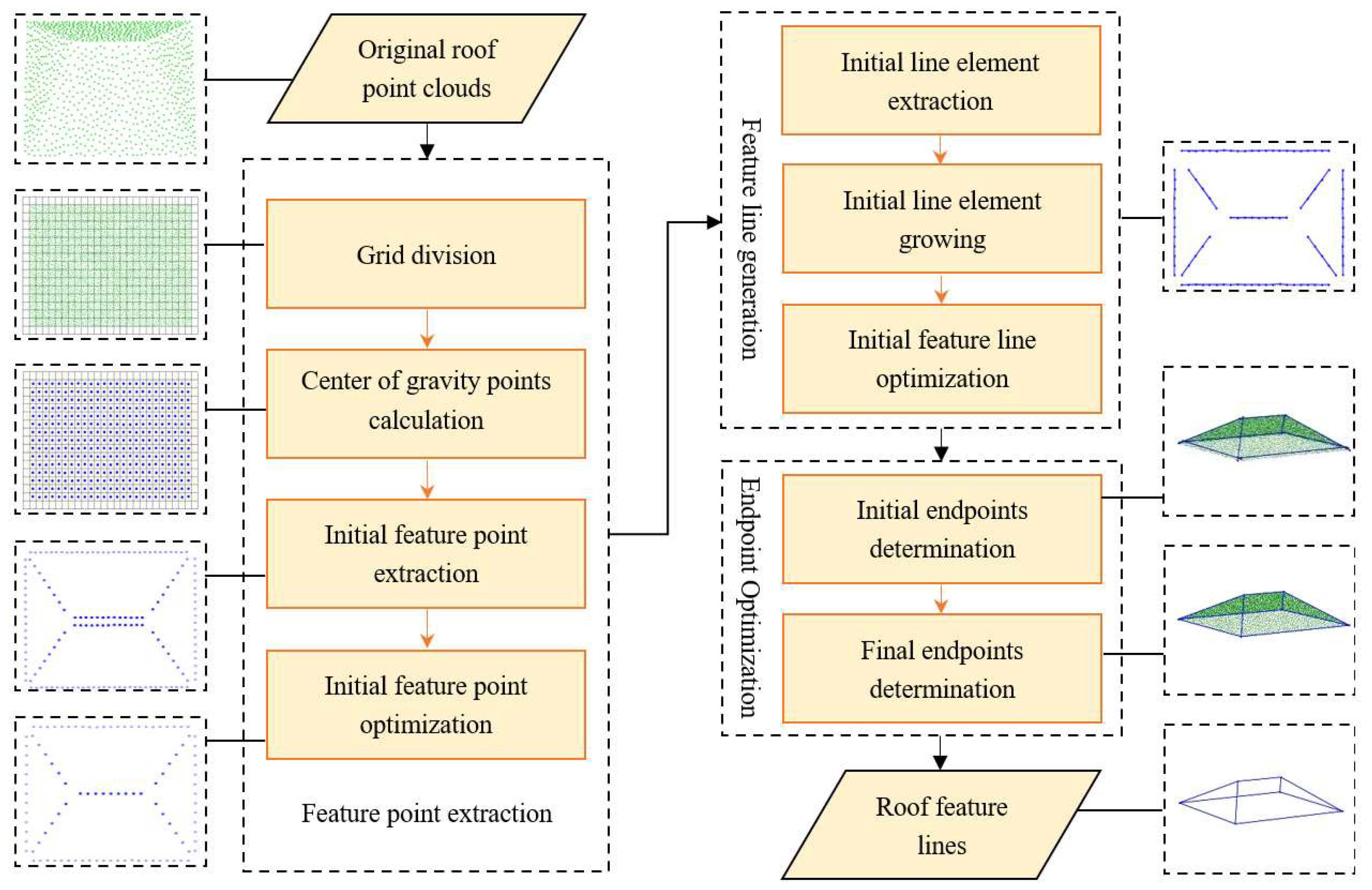
The remainder of this paper is organized as follows. Section 2 introduces the basic principle of the proposed algorithm, including the extraction and optimization of initial feature points, extraction of line segment elements and feature line generation, and determination and optimization of the endpoint. Section 3 outlines the experiments. The proposed algorithm was applied to extract the roof feature lines of four single buildings and a group of regional buildings. The results were compared with the feature line extraction results of other algorithms, thus verifying the effectiveness of the proposed algorithm. Section 4 and Section 5 present the discussion and conclusions, respectively.

2. Methods

The proposed feature line extraction algorithm for roof point clouds, based on the linear distribution characteristics of neighborhood points, was comprised of three main stages: feature point extraction, feature line generation, and feature line endpoint optimization. In the stage of feature point extraction, the neighborhood relationship between points was established by gridding the 3D space. The feature points were determined according to the linear relationship between the center of gravity in the current grid and the center of gravity in the neighbor grids. The initial feature points were optimized for the second time by using grids of different scales. The stage of feature line generation can be further divided into the extraction of the initial line segment elements, growth of the initial line segment elements, and combination and optimization of the feature lines. First, the initial segment elements were determined according to the space angle between two vectors formed by the current feature point and two feature points in the neighborhood. The points collinear with the initial segment element were determined by the distance from other feature points to the initial segment element, thus realizing the growth of the segment element. Later, the initial feature line was extracted through fitting the optimization of the segment element after growth. In the stage of feature line endpoint optimization, based on determining the types of inner and outer feature lines, first, the outer point with the furthest vertical distance from the feature line among the original points near each endpoint of the outer feature line was chosen to determine the distance of the outer feature line translating outward, so that the outer feature line was vertically translated outward on the horizontal plane. Then, by calculating the intersection point of the straight line and determining the point nearest to the intersection point, the endpoints of the feature lines belonging to the corresponding endpoints were optimized as a whole. Finally, the optimization of feature line endpoints was completed. The overall flow of the algorithm is shown in Figure 2.

2.1. Extraction of Feature Points

As described in Section 1, the building roof feature lines include the outer and inner feature lines. According to the arrangement features of points on a straight line, points on the same line are in a linear distribution, as shown by points a, b, and c in Figure 3a. It can be seen from the analysis that points on the feature line in the ideal case were characterized by the uniqueness of their linear arrangement. Due to the uneven density and discrete distribution of the airborne LiDAR point cloud data, a virtual grid was used in this paper to rasterize the point clouds, and the centers of gravity of the grids were used instead of the original points to analyze the linear distribution characteristics.

The uniqueness of the linear arrangement of points on the roof feature line can be reflected by the three-dimensional vector angle formed by the center of gravity of the points in the current grid with the centers of gravity of the two neighboring grids. As shown in Figure 3a, point b was the center of gravity of a grid on any feature line, and, among all the included angles formed by point b and any two centers of gravity in its eight-neighborhood grids, only one angle $〈\overrightarrow{\mathrm{b}\mathrm{a}},\overrightarrow{\mathrm{b}\mathrm{c}}〉$ was close to 180°, i.e., point b satisfied the characteristics of linear arrangement uniqueness. In contrast, among the three-dimensional angles formed by the center of gravity of a grid within a non-edge region of the roof surface and the centers of gravity of any two adjacent grids in the eight-neighborhood grids, there were many angles close to 180°. In other words, there were multiple linear distributions. As shown by the dotted lines in Figure 3b, there were four angles close to 180°. Based on the above features, a feature line extraction algorithm for building roofs based on the distribution characteristics of neighboring points was proposed. This algorithm can be applied to both edge contour points and internal ridge points.

2.1.1. Establishment of Virtual Grids

The original point clouds of the roof were projected onto the XOY plane, and the coverage of the virtual grid was determined according to the maximum and minimum values of the coordinates of the point cloud data in the X and Y directions. The grid size is the key to the point cloud division: if the grid size is too small, it will lead to too few points in the grid and too many empty grids, which is unfavorable to the extraction of feature points. If the grid size is too large, the number of extracted feature points will be too small, which is unfavorable to the subsequent fitting process. Considering the inconsistency of the density of different point cloud data, in this paper, we adopted the average point spacing d as the adaptive factor of the grid size, which was used to improve the adaptability of the algorithm to different density point clouds. A virtual grid with side length L was used to spatially divide the point clouds, and the grid division formula was as follows:

$$\left\{\begin{array}{c}{R}_c=int\left({\displaystyle \frac{X_{\mathit{max}}-X_{\mathit{min}}}{L}}\right)+1\\ C_c=int\left({\displaystyle \frac{Y_{\mathit{max}}-Y_{\mathit{min}}}{L}}\right)+1\end{array}\right.$$

(1)

where $R_c$ and $C_c$ are the number of grids in the X and Y directions, respectively. $\mathit{int}\left(\right)$ is the upward rounding function. $X_{\mathit{max}}$, $X_{\mathit{min}}$, $Y_{\mathit{max}}$, and $Y_{\mathit{min}}$ are the maximum and minimum coordinate values of the point cloud data in the X and Y directions, respectively.

2.1.2. Center of Gravity Points Calculation

Under these circumstances, there was a uniform distribution of points in the grid. The center of gravity could reflect the distribution characteristics of the original points within the grid. For each non-empty grid, the center of gravity of all points in the grid was used to replace original points in the grid, and this was used to analyze the linear distribution characteristics of the points in the neighborhood grids. The formula for calculating the center of gravity of points in the grid was as follows:

$$\left(\stackrel{\mathrm{-}}{\mathit{x}},\stackrel{\mathrm{-}}{\mathit{y}},\stackrel{\mathrm{-}}{\mathit{z}}\right)=\left({\displaystyle \frac{1}{\mathit{n}}}\sum _{\mathit{i}=1}^{\mathit{i}=\mathit{n}}{\mathit{x}}_{\mathit{i}},{\displaystyle \frac{1}{\mathit{n}}}\sum _{\mathit{i}=1}^{\mathit{i}=\mathit{n}}{\mathit{y}}_{\mathit{i}},{\displaystyle \frac{1}{\mathit{n}}}\sum _{\mathit{i}=1}^{\mathit{i}=\mathit{n}}{\mathit{z}}_{\mathit{i}}\right)$$

(2)

where $\left(\stackrel{\mathrm{-}}{\mathit{x}},\stackrel{\mathrm{-}}{\mathit{y}},\stackrel{\mathrm{-}}{\mathit{z}}\right)$ are the coordinates of the center of gravity, and n is the number of original points in a grid.

2.1.3. Initial Feature Point Extraction

Based on the grid after rasterization, the specific principle of extracting feature points based on the linear distribution of the center of gravity points of the current grid and neighboring grids was as follows:

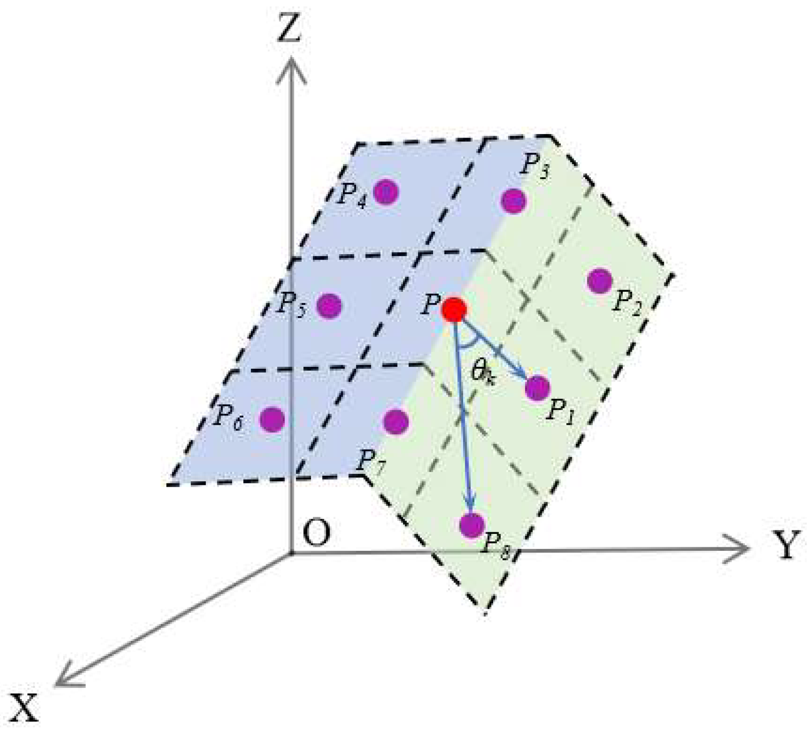
• As shown in Figure 4, any non-empty grid was chosen as the current grid and its center of gravity was recorded as P. The center of gravity set of non-empty grids in the eight-neighborhood was $\mathsf{\Omega }=\left\{{\mathit{P}}_1,{\mathit{P}}_2,\dots \right.,\left.{\mathit{P}}_{\mathit{m}}\right\}$, where m is the number of non-empty grids in the eight-neighborhood. It is worth noting that when $\mathit{m}=1$, it means that there is only one non-empty grid in the eight-neighborhood of the current grid, and the three-dimensional angle cannot be formed. Only when $2\le \mathit{m}\le 8$ can the centers of gravity ${\mathit{P}}_{\mathit{i}}$ and ${\mathit{P}}_{\mathit{j}}$ of any two non-empty grids be chosen randomly in the eight-neighborhoods of the current grid, where i, j belong to $\left\{1,2,3,\dots \right.,\left.\mathit{m}\right\}$ and $\mathit{i}\ne \mathit{j}$. According to Equation (3), the three-dimensional angle ${\theta }_{\mathit{k}}=〈\overrightarrow{{\mathit{PP}}_{\mathit{i}}},\overrightarrow{{\mathit{PP}}_{\mathit{j}}}〉$ was calculated.

  $${\theta }_{\mathit{k}}=\mathit{arccos}\left({\displaystyle \frac{\overrightarrow{{\mathit{PP}}_{\mathit{i}}}·\overrightarrow{{\mathit{PP}}_{\mathit{j}}}}{‖\overrightarrow{{\mathit{PP}}_{\mathit{i}}}‖‖\overrightarrow{{\mathit{PP}}_{\mathit{j}}}‖}}\right)$$

  (3)
• Under the above conditions, the three-dimensional angle set formed by the center of gravity in the current grid and any two centers of gravity in the eight-neighborhood was $\vartheta =\left\{{\theta }_1,{\theta }_2,\dots \right.,\left.{\theta }_{\mathit{k}}\right\}$, where $\mathit{k}={\mathit{C}}_{\mathit{m}}^2$. This was the total number of formed angles. According to Equation (4), the number ${\mathit{N}}_{\theta }$ of three-dimensional angles in the set $\vartheta$ that were larger than the angle threshold ${\mathit{T}}_{\theta }$ was ${\mathit{N}}_{\theta }$. If ${\mathit{N}}_{\theta }=1$, the center of gravity in the current grid is the feature point. In this study, it was set ${\mathit{T}}_{\theta }=170°$.

  $${\mathit{N}}_{\theta }=\sum _{\mathit{q}=1}^{\mathit{q}=\mathit{k}}{\mathit{N}}_{\mathit{q}}\left\{\begin{array}{c}\mathit{if} {\theta }_{\mathit{q}}>{\mathit{T}}_{\theta }, {\mathit{N}}_{\mathit{q}}=1\\ \mathit{if} {\theta }_{\mathit{q}}\le {\mathit{T}}_{\theta }, {\mathit{N}}_{\mathit{q}}=0\end{array}\right.$$

  (4)
• Based on the above principle, all non-empty grids were traversed successively, and all qualified centers of gravity were added to the initial feature point set.

2.1.4. Initial Feature Point Optimization

In the process of feature point extraction, the inner feature points of the roof, such as the feature points at the ridge, are projected onto two rows of adjacent grids alternately due to the influence of grid size. The feature point extraction results may occur in two rows of feature points representing the same feature line, as shown by the points of the black box in Figure 5a.

Theoretically, feature points on the same feature line will be collinear. Hence, the initial feature point extraction results were optimized by the secondary grid division. The specific method was as follows: secondary grid division was performed on the initial feature point set with two times the grid size, i.e., with the grid size of 2L. For a grid containing multiple initial feature points, the center of gravity of the initial feature points in the grid was used to replace the original feature points, obtaining refined results for the initial feature points, as shown by the red points in Figure 5b.

2.2. Extraction of Feature Lines

The feature points extracted in the above process inherited the disorderedness of the point clouds, and there was a semantic missing problem. Based on the feature point extraction results, the initial feature lines were extracted using three steps: initial segment element extraction, initial segment element growth, and feature line optimization.

Extraction of the initial segment element. As shown in Figure 6, any feature point k_m can be taken as an example, and two feature points, k_m−1 and k_m+1, nearest to k_m, were chosen. k_m was used as the angular point. The three-dimensional angle α formed by the two vectors $\overrightarrow{{\mathit{kk}}_{\mathit{m}-1}}$ and $\overrightarrow{{\mathit{kk}}_{\mathit{m}+1}}$ was calculated according to Equation (3). If ${\alpha >\mathit{T}}_{\theta }$, the segment formed by k_m, k_m−1, and k_m+1 was used as an initial segment element; that is, the initial seed segment. The initial segment element extraction operation was performed for each feature point in the set to obtain all possible initial segment elements. Each segment element corresponded to an initial point set consisting of three points.

Growth of the initial segment element. First, the initial line equation was obtained by fitting the initial point set using the least squares method. Secondly, the distances from other feature points to the straight line were calculated, and points with distances less than L were added to the initial point set to complete the first expansion of the point set. The RANSAC algorithm was used to generate the feature line from the expanded point set. Specifically, two points were randomly selected from the expanded point set. The straight line connecting these two points was calculated, and the distances from the remaining points to the straight line were calculated. The points with distances less than L were recorded as the inner points of the current straight line. This process was repeated by iterating n times. The straight line with the largest proportion of inner points was taken as the representative straight line for the point set. Finally, we repeated the previous step until the growth of the initial line segment element was completed, which occurred when no new feature points were added to the initial point set. We repeated the whole process described above for the remaining initial line segment elements until all initial line elements had been processed, where each initial line segment element corresponded to a point set and a straight line, noted as the initial feature line. To ensure that the results of the RANSAC-fitted straight line were optimal, we set a larger n = 80.

Optimization of initial feature lines. In the above extraction results of the initial feature lines, each initial feature line corresponded to a point set. Whether two lines were on the same feature line was judged by calculating the collinear probability between two point sets. The compatibility of any two lines could be calculated using Equation (5). As shown in Figure 6, we supposed two point sets corresponding to any two initial feature lines ${\mathit{L}}_{\mathit{A}}$ and ${\mathit{L}}_{\mathit{B}}$ are $\mathrm{A}=\left\{{\mathit{a}}_1,{\mathit{a}}_2,\dots \right.,\left.{\mathit{a}}_{\mathit{m}1}\right\}$ and $\mathrm{B}=\left\{{\mathit{b}}_1,{\mathit{b}}_2,\dots \right.,\left.{\mathit{b}}_{\mathit{m}2}\right\}$, where m1 and m2 are the number of points in two sets, respectively. The longer of the two initial feature lines was chosen as the reference, and if the length of line ${\mathit{L}}_{\mathit{A}}$ was greater than the length of line ${\mathit{L}}_{\mathit{B}}$, the calculation formula for the compatibility of the two lines was as follows:

$$\mathit{C}(\mathit{A},\mathit{B})=\mathit{max}\left({\displaystyle \frac{\sum _{\mathit{j}=1}^{\mathit{j}=\mathit{m}2}{‖\mathit{max}\left(\mathit{dis}\left({\mathit{L}}_{\mathit{A}},{\mathrm{b}}_{\mathit{j}}\right),\mathit{L}\right)‖}_{\mathit{L}}}{\mathit{m}2/2}}-1,0\right)$$

(5)

where $\mathit{dis}\left(\right)$ is the point-to-line distance function and $\mathit{max}\left(\right)$ is the maximum function. $‖\mathit{n}‖$ is a function that determines whether n is less than L. The numerator expresses the number of points in B whose distance to feature line A is less than L.

If C > 0, the compatibility of the initial feature lines corresponding to two point sets was high, and the two lines were collinear lines. Points in two sets were combined. All feature lines were traversed until the compatibility between any two feature lines was equal to 0. The feature line fitting was carried out for the updated point sets, giving the final feature line extraction results.

2.3. Determination of the Endpoints of the Feature Line

Building roofs have diversified shapes. When there was a collineation of several nonadjacent feature lines on the roof, as in Figure 7, the extraction results of the red and green feature lines corresponded to the same line equation. Therefore, we first had to divide the points on the feature lines corresponding to the line equation into several groups during the specification of the feature line.

2.3.1. Determination of the Initial Endpoints of the Feature Line

The original points in the grid where the feature points are located were projected onto the corresponding feature line. Projection points were ranked according to their distances to the origin of the coordinate system, and the three-dimensional distance D between two adjacent projection points was judged successively. If D > 1 m, these two adjacent points were recorded as the endpoints of two different segments. As shown in Figure 8, points a₁-j₁ were the projection points of the origin points on the feature line L. If the distance between c₁ and d₁ was larger than 1 m, the projection points were split into two ordered point sets of a₁-c₁ and d₁-j₁. The above splitting process was repeated for the split point sets until the distance of adjacent points in each point set was less than 1 m. Under these circumstances, the front and back ends of each ordered point set were used as two endpoints of a segment, giving the initial feature line segments.

2.3.2. Optimization of the Initial Endpoints

Since the feature point is the center of gravity of the grid, the feature line generated by fitting the center of gravity has an overall inward shrinkage phenomenon compared with the actual feature line, in which the outer feature line translation is mainly reflected in three directions, while the inner feature line translation is mainly reflected in the elevation deviation. Therefore, to obtain more accurate corner points of the building roof, in this paper, we optimized the feature line endpoints based on the original points in the neighborhood of the initial endpoints.

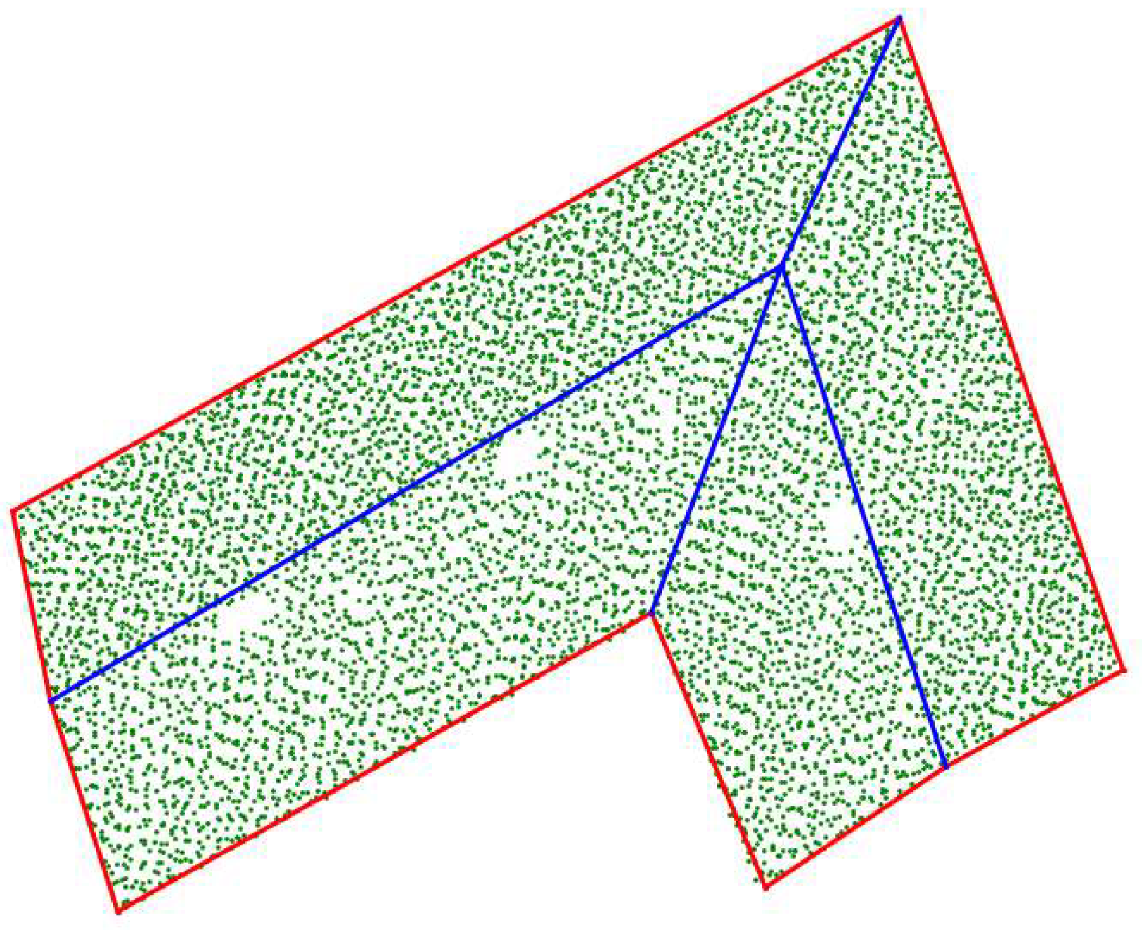
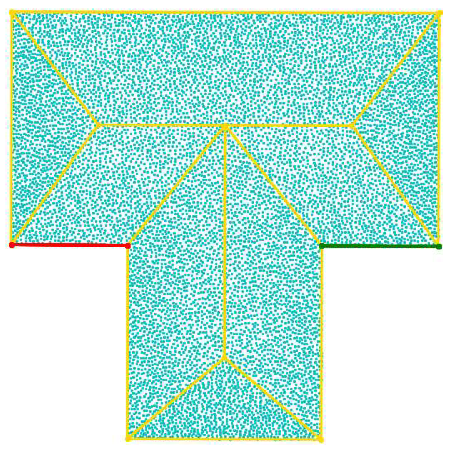
• Classification of feature lines. A feature line was considered to be an outer feature line if there were empty grids in the eight-neighborhood of the grids where the two endpoints of the feature line were located, as shown by the blue line in Figure 9; otherwise, the feature line was considered to be an inner feature line, as shown by the red line in Figure 9.
• Optimization of outer feature lines. As shown in Figure 10, for any outer feature line ${\mathit{L}}_{\mathit{k}}$, with initial endpoints ${\mathit{k}}_1$ and ${\mathit{k}}_2$, a circular region with radius L was constructed on the horizontal plane with one of its side endpoints ${\mathit{k}}_1$ as the center of the circle, and the circular region was equally divided into two semicircles along the direction of the feature line. The number of original points with x and y coordinates located in the two semicircles was counted, and the side with fewer points was considered to be the outer side of the feature line. The distances from all original points located in the outer semicircle to the line where the feature line was located were calculated, and the farthest distance among them was determined to be ${\mathit{d}}_1$. Similarly, the farthest distance from the original points in the outer semicircle constructed with the other endpoint ${\mathit{k}}_2$ of the feature line ${\mathit{L}}_{\mathit{k}}$ to the feature line was obtained as ${\mathit{d}}_2$. Calculating the translation distance ${\mathit{d}}_3=\left({\mathit{d}}_1+{\mathit{d}}_2\right)/2$, the feature line was translated vertically outward by the distance ${\mathit{d}}_3$ in the horizontal plane, and the translated feature line and its endpoints ${{\mathit{d}}_1}^{\prime }$ and ${{\mathit{d}}_3}^{\prime }$ were obtained.
• Optimization of the corresponding endpoints. We calculated the distance between the endpoints of different feature lines. The initial endpoints with a distance between each other of less than 3L were recorded as a group of corresponding endpoints and were optimized, and the coordinates of the optimized endpoints were marked as (X, Y, Z). If the number of endpoints in the group N = 2, the coordinates of the intersection of the two feature lines where the two endpoints were located were taken as the X and Y coordinates of the optimized endpoints, and the elevation of the original point nearest to the intersection was used as the Z coordinate, thus completing the optimization of the corresponding endpoints in the group. If N > 2, the intersection points were calculated for any two feature lines with a large difference in slope, and the means of the coordinates of all the intersection points were calculated as the X and Y coordinates of the optimized endpoints. The elevation of the original point nearest to the mean point was used as the Z coordinate, thus completing the optimization of the corresponding endpoints in this group.

3. Experimental Results and Analysis

3.1. Experimental Data

To verify the effectiveness of the proposed algorithm, the Estonian City dataset [31] and the analog dataset were chosen for experiments of feature line extraction from building roof point clouds.

The Estonian City dataset was obtained by extracting the building roofs from the original point cloud data provided by the Land Board of the Republic of Estonia. The original LiDAR point cloud data were acquired by a high-precision RIEGL VQ-1560i scanner at an altitude of 2600 m. The relative accuracy of the points in the dataset was 20 mm, the average point density was 30.314 points per square meter, and the average point spacing was 0.1816 m. The dataset also provided standard building roof wireframes as reference data, which had an average displacement of 0.065 m from the original point cloud data. In this paper, the roof point clouds of eight buildings with different complexities of roofs in the Estonian City dataset were selected for the feature line extraction experiments, as shown in Figure 11a. The data quality of R1–R6 was better. There was a large number of accessory structures on the roof of the building R7, which resulted in dense noise in the roof surface point cloud. There may have been tall trees in the vicinity of R8, which resulted in scattered noise on the roof.

The analogue dataset was the point cloud data of multiple building roofs in gable, four-slope, four-slope T-shaped, and four-slope L-shaped designs, generated using CloudCompare2.13.1 software based on common roof structures, as shown in Figure 11b. The average point density of this dataset was 54.626 points per square meter, and the average point spacing was 0.1059 m.

3.2. Analysis of Experimental Parameters

We performed feature line extraction based on the results of feature point extraction. The feature point extraction results were the key to feature line extraction, directly determining the quality of the feature line extraction results. The grid size L and angle threshold ${\mathit{T}}_{\theta }$ had a crucial impact on the feature point extraction results.

To determine the optimum grid size, we calculated the distance ${\mathit{M}}_{\mathit{d}}$ from the center of gravity of each grid to the center of the grid and the mean value of all the distances $\overline{{\mathit{M}}_{\mathit{d}}}$. The stability of the center of gravity was reflected by calculating the value of Dr, ${\mathit{D}}_{\mathit{r}}=\overline{{\mathit{M}}_{\mathit{d}}}/\mathit{k}$, where k is the maximum offset value from the center of gravity to the center in the grid, i.e., $\mathit{k}=\sqrt{\mathit{L}}/2$. The larger Dr was, the more the center of gravity was off from the center of the grid and the lower its stability. The smaller Dr was, the higher the stability of the center of gravity and the stronger the uniqueness of the linear arrangement of the center of the gravity points of the grids where the feature line was located. Figure 12 shows the Dr values calculated using different grid sizes for the grid division of the six sets of data in Figure 11a. The Dr values showed a decreasing trend as the grid size L increased. Specifically, when $\mathit{L}<4\mathit{d}$, the Dr value showed a rapid decreasing trend as L increased; when $\mathit{L}>4\mathit{d}$, the Dr value tended to level off. This indicated that the distance from the center of gravity to the center of the grid tended to be stable when $\mathit{L}=4\mathit{d}$. In addition, the grid size was inversely proportional to the number of feature points extracted and the extraction accuracy. As a result, we set the grid size to $\mathit{L}=4\mathit{d}$.

Ideally, the points of the feature line of the building roof would be strictly in line with the single-direction linear distribution, i.e., satisfying ${\mathit{T}}_{\theta }=180°$. However, since point cloud data collected by LiDAR are discrete and do not have completeness and absolute flatness, the angle formed by three neighboring points on the collected feature line was generally less than 180°.

To determine the optimal angle threshold ${\mathit{T}}_{\theta }$ for feature line extraction, we took the R4 data in Figure 11a as an example and performed feature point extraction on the building roof point clouds with different values of ${\mathit{T}}_{\theta }$. The extraction results are shown in Figure 13. With the gradual increase in the angle threshold ${\mathit{T}}_{\theta }$, the number of feature points extracted gradually increased. When the angle threshold ${\mathit{T}}_{\theta }<170°$, the extracted points on the feature line were too sparse to realize the effective expression of the roof feature line. When the angle threshold ${\mathit{T}}_{\theta }>170°$, there were too many noise points extracted from the interior of the roof surface, which seriously interfered with the generation of the following feature line. When the angle threshold ${\mathit{T}}_{\theta }=170°$, the extracted feature points were more dense and there were few noise points. The extraction results were optimal, so we set ${\mathit{T}}_{\theta }=170°$.

3.3. Evaluation Measures

To quantitatively analyze the feature line extraction results of different algorithms, based on the standard wireframe data, the evaluation metrics in [24] were utilized to quantitatively analyze the roof feature line extraction results. This process evaluated the extraction results mainly by calculating the comprehensive similarity between the feature lines extracted by different algorithms and the reference feature lines, as shown in Equation (9). It comprehensively considered the three aspects of distance similarity, orientation similarity, and projection similarity measures. The calculation formulas are shown in Equations (6)–(8), respectively. In Figure 14, the reference feature line AB and the extracted feature line CD are given. Points C₁ and D₁ are the projection points of the endpoints of segment CD on the segment AB. α is the included angle between segment AB and segment CD.

The calculation formulas of the above three similarity measures were as follows:

• Distance similarity (ds, dis = 0.2 m):

$$\mathit{ds}=\mathit{exp}\left\{\left.-{\left({\displaystyle \frac{\left|\mathit{C}{\mathit{C}}_1\right|+\left|\mathit{D}{\mathit{D}}_1\right|}{\left|2·\mathit{dis}\right|}}\right)}^2\right\}\right.$$

(6)

2.

Direction similarity (os, α₀ = 5°):

$$\mathit{os}=\mathit{exp}\left\{\left.-{\left({\displaystyle \frac{\alpha }{{\alpha }_0}}\right)}^2\right\}\right.$$

(7)

3.

Projection similarity (ps):

$$\mathit{ps}={\displaystyle \frac{\left|\mathit{AB}\right|\cap \left|{\mathit{C}}_1{\mathit{D}}_1\right|}{\left|\mathit{AB}\right|\cup \left|{\mathit{C}}_1{\mathit{D}}_1\right|}}={\displaystyle \frac{\left|{\mathit{C}}_1{\mathit{D}}_1\right|}{\left|\mathit{AB}\right|}}$$

(8)

On this basis, the comprehensive similarity cs of all feature lines contained on each building roof was calculated according to Equation (9). The total number of feature lines of a single roof was given as m, and j was the jth feature line on the roof.

$$\mathit{cs}={\displaystyle \frac{\sum _{\mathit{j}=1}^{\mathit{j}=\mathit{m}}{\mathit{ds}}_{\mathit{j}}·{\mathit{os}}_{\mathit{j}}·{\mathit{ps}}_{\mathit{j}}}{\mathit{m}}}\times 100\mathrm{\%}$$

(9)

3.4. Results

To verify the effectiveness of the proposed algorithm, the feature line extraction experiments were conducted on R1 to R8 data using the proposed method, the method in [21], and the method in [25]. The feature line extraction results of the three algorithms were compared and analyzed.

In contrast to the proposed algorithm, the algorithms in [21,25] employed different strategies for extracting various types of feature lines on building roofs. In [21], roof feature lines were categorized into three types: roof outlines, normal ridge lines, and oblique ridge lines. Then, distinct extraction methods for each type were proposed, including (1) initial contour point extraction and outline generation based on boundary grids; (2) normal ridge line generation using a combination of initial contour points and elevation constraints; and (3) inclined ridge line extraction based on curvature feature constraints. Key parameters for these methods included a grid size that was twice the average point spacing, a growing search radius that was 2–3 times the average point spacing, and a curvature threshold that was twice the average curvature of all points.

In [25], the outer contour of the roof was extracted using the Alpha Shapes algorithm with the rolling circle radius set to two times the average point spacing. The roof ridge was obtained by intersecting the roof surfaces obtained by segmentation using the RANSAC algorithm. During the segmentation process, the point-to-plane distance threshold was set to 0.1 m, the number of iterations was set to 200, and the minimum number of points required for plane fitting was 3.

3.4.1. Feature Line Extraction Results of Different Algorithms

Figure 15 shows the results of feature line extraction on the R1–R8 point cloud data by different algorithms. Both the proposed algorithm in this paper and the algorithm outlined in [25] were able to extract the complete building roof feature lines without false extractions and omissions. The algorithm outlined in [21] had obvious errors in the results of the inner feature line extraction for the R3–R7 data.

The errors could be categorized into two types. One type was generated during the extraction process of the normal ridge line, as shown by the yellow lines in Figure 15. This type of error manifested as noticeable overgrowth or over-connection. This issue arose because the process of determining the topological relationships between adjacent lines, based on point attribution, incorrectly identified originally non-intersecting lines as intersecting lines. The other was errors during inclined ridge line generation, represented by the black lines in Figure 15. This error occurred when two symmetrical oblique ridge lines were extracted but replaced by a horizontal line. This problem resulted from the algorithm in [21], which projected the extracted feature points onto the 2D horizontal plane and grouped them according to the collinearity constraints to extract the feature lines. Since the two symmetric inclined ridges projected onto the 2D horizontal plane satisfied the collinearity condition, the points on these two oblique ridge lines were grouped together, leading to the generation of a straight line obtained by linear fitting.

Furthermore, although the algorithm outlined in [25] had no significant error in the feature line extraction results for R1–R8, its endpoint accuracy was slightly lower. This was because, in [25], different methods were used to determine the final endpoint coordinates for different types of roofs. For example, for simple roof types such as herringbone, four-cornered pointed roofs, and the four-slope shape, in [25], the elevation Z of the highest or lowest point among all the points was selected as the elevation of different endpoints of the feature line based on determining the planar coordinates of the endpoints. This method did not consider the overall distribution of the neighboring feature points, which led to the existence of an outward expansion of some feature lines, as shown in the black boxes of R1–3 in Figure 15. For roofs with complex structures, in [25], only the points in the contour points that formed an angle of more than a given threshold with the neighboring points on both sides as the endpoints of the roof were selected, and the subsequent optimization of the endpoints was not carried out, which led to a large deviation between some of the endpoints and the real endpoint locations if the quality of the data at the roof corners was poor, as shown by the black boxes for R4–R8 in Figure 15.

The proposed algorithm in this paper avoided the errors caused by 2D grouping by judging the collinearity of the extracted 3D feature points in three-dimensional space. Additionally, to ensure the accuracy of the feature line endpoints, we adopted different methods to optimize the endpoints of the inner and outer feature lines, respectively, to solve the phenomenon of the overall inward shrinkage of the feature lines caused by the center of gravity of the grid. Since the proposed algorithm adopted the 3D angle between the center of gravity of the non-empty grid and the center of gravity of two non-empty grids within its eight-neighborhood as the judgment condition for the linear distribution characteristics, it had a certain degree of tolerance for the noise in each grid, thus ensuring the stable extraction of feature lines. As can be seen in Figure 15, the feature lines extracted by the proposed algorithm had a higher accuracy.

In [25], different extraction strategies for the feature line extraction for two different types of roofs, simple and complex, were used, and it was not possible to extract the feature lines of multiple buildings consisting of different types of roofs at the same time. Therefore, for area point clouds containing multiple buildings, as in Figure 11b, only the feature line extraction results obtained by the proposed algorithm were compared and analyzed with the method in [21], and the results are shown in Figure 16. There were obvious errors in the extraction results of [21], as shown by the black line in Figure 16. The proposed algorithm does not require the individual segmentation of the building point clouds and is able to extract the feature lines from point clouds containing multiple buildings. The feature line extraction results were therefore more accurate and achieved a better visual effect.

3.4.2. Quantitative Analysis of the Feature Line Extraction Results

To quantitatively assess the feature line extraction results of different algorithms, the similarity of these results was evaluated using the method described in Section 3.3.

Table 1. Comprehensive similarity between feature lines extracted by different algorithms and the reference feature lines (%).

	R1	R2	R3	R4	R5	R6	R7	R8	R9
Reference [21]	82.95	84.14	40.25	52.69	60.16	55.78	59.63	85.69	73.69
Reference [25]	79.76	82.43	81.58	83.08	80.06	81.08	84.96	83.46	-
Ours	91.84	88.79	89.62	88.24	89.48	88.92	89.03	90.31	92.70

presents the comprehensive similarity statistics of feature lines extracted by different algorithms for the R1–R8 point cloud data, compared with reference feature lines. The results indicated that the feature lines extracted by the proposed algorithm exhibited the highest similarity to the reference feature lines, achieving a similarity rate exceeding 88% across all datasets. Compared to the comprehensive similarity cs values of the feature lines extracted by the algorithms in [21,25], the proposed algorithm showed an improvement ranging from 4.07% to 49.37%. For the point cloud data R9, the comprehensive similarity of feature lines extracted by our algorithm reached 92.70%. These results demonstrated the effectiveness and superiority of the proposed algorithm. In addition, the proposed algorithm achieved the highest cs value for the simulated point clouds with the highest density, which indicated that it performed better with denser point cloud data and offered greater stability.

4. Discussion

To evaluate the effect of different densities on the processing efficiency and accuracy of the proposed algorithm, we constructed a surface model with a herringbone roof structure and extracted point clouds with different densities on the modeled roof using the CloudCompare2.13.1 software, as shown in Figure 17, N1–N8. The mean square error of the coordinates of all the corner points of the roof was used as a measure of the accuracy of the feature line extraction results. A smaller mean square error indicated more accurate extraction results. References [21,25] and the proposed algorithm were used for feature line extraction, respectively. The running time and accuracy of the extraction results of the three algorithms are shown in Figure 18 and

Table 2. The mean square error of coordinates for corner points in N1 to N8 (units: meters).

	N1	N2	N3	N4	N5	N6	N7	N8
Reference [21]	0.0091	0.0085	0.0078	0.0071	0.0068	0.0061	0.0057	0.0052
Reference [25]	0.0084	0.0081	0.0073	0.0065	0.0060	0.0056	0.0052	0.0049
Ours	0.0086	0.0082	0.0075	0.0070	0.0067	0.0059	0.0055	0.0051

, respectively.

In [21], a point-by-point analysis of the curvature and spatial location features was required, which led to a sharp increase in the time required for extracting feature lines when the density of the raw data points increased, as shown by the red curve in Figure 18. Therefore, the method is not suitable for the extraction of feature lines for a large number of points. The authors of [25] used the Alpha Shapes method to extract the contour points; however, an exponential growth trend was maintained with an increasing density of points, as shown by the green curve in Figure 18. The proposed algorithm used the center of gravity points after the virtual grid division for feature line extraction, which effectively reduced the number of samples involved in the computation. At the same time, the use of linear distribution characteristics was able to realize the simultaneous extraction of inner and outer feature lines. Therefore, with the increase in the density of points, the running time of the proposed algorithm showed a linear rising trend, and the time required was always the shortest when feature line extraction was carried out on point cloud data with different densities of points, as shown by the blue line in Figure 18.

In Table 2, for point cloud data with different densities, the accuracy of the extraction results of all three algorithms increased as the point density increased. Reference [25] showed the highest accuracy for data with different densities of points, while reference [21] achieved the lowest accuracy. Therefore, the combined running time and accuracy results showed that the proposed algorithm was effective.

Although the experimental results demonstrated the effectiveness and applicability of the proposed algorithm, certain limitations remained. For example, we used the linear distribution characteristics of the grid’s center of gravity to extract feature points and generate feature lines. However, for the extraction of shorter building roof feature lines in complex urban scenes, the support of higher point density is often required.

5. Conclusions

A feature line extraction algorithm for roof point clouds based on the linear distribution characteristics of neighborhood points was proposed in this paper. Experiments were conducted using a dataset containing eight single building point clouds and a dataset containing multiple buildings, yielding complete and accurate feature line extraction results. The proposed algorithm had the following characteristics:

(i)

Enhanced robustness: The algorithm analyzed the linear distribution characteristics of local neighborhood points based on the center of gravity of the grid, rather than the original points. This approach enhanced the robustness of point clouds of varying densities and mitigated the impact of noise points on the extraction results.

(ii)

Direct extraction of 3D features: The algorithm directly extracted 3D feature points and feature lines in the object space. This improved the effectiveness and reliability of feature line extraction by effectively leveraging the local structural features and 3D information of the point clouds.

(iii)

Endpoint optimization: Based on the extracted feature lines from the center of the gravity points, the algorithm optimized the endpoints and merged the corresponding endpoints. This optimization addressed the issue of the inward shrinkage of the extracted feature lines compared to the actual feature lines.

Currently, the results of the proposed algorithm are limited to visual feature line extraction and lack the topological relationships between lines and between lines and surfaces. Future research will focus on extracting shorter feature lines from complex buildings and constructing the topological relationships between lines to develop a roof wireframe model of the building, completing the three-dimensional reconstruction of the building model based on the results of this research.

References

1. Yu, D.W.; Ji, S.P.; Liu, J.; Wei, S.Q. Automatic 3D building reconstruction from multi-view aerial images with deep learning. ISPRS J. Photogramm. Remote Sens. 2021, 171, 155–170. [Google Scholar] [CrossRef]
2. Li, M.L.; Nan, L.L.; Smith, N.; Wonka, P. Reconstructing building mass models from UAV images. Comput. Graph. 2016, 54, 84–93. [Google Scholar] [CrossRef]
3. Huang, J.; Stoter, J.; Peters, R.; Nan, L.L. City3D: Large-Scale Building Reconstruction from Airborne LiDAR Point Clouds. Remote Sens. 2022, 14, 2254. [Google Scholar] [CrossRef]
4. Pahlavani, P.; Amirkolaee, H.A.; Bigdeli, B. 3D reconstruction of buildings from LiDAR data considering various types of roof structures. Int. J. Remote Sens. 2017, 38, 1451–1482. [Google Scholar] [CrossRef]
5. Li, Z.X.; Shan, J. RANSAC-based multi primitive building reconstruction from 3D point clouds. ISPRS J. Photogramm. Remote Sens. 2022, 185, 247–260. [Google Scholar] [CrossRef]
6. Zhang, W.Y.; Li, Z.X.; Shan, J. Optimal Model Fitting for Building Reconstruction From Point Clouds. IEEE J. Sel. Top. Appl. Earth. Observ. Remote Sens. 2021, 14, 9636–9650. [Google Scholar] [CrossRef]
7. Li, L.; Song, N.; Sun, F.; Liu, X.Y.; Wang, R.S.; Yao, J.; Cao, S.S. Point2Roof: End-to-end 3D building roof modeling from airborne LiDAR point clouds. ISPRS J. Photogramm. Remote Sens. 2022, 193, 17–28. [Google Scholar] [CrossRef]
8. Poullis, C. A Framework for Automatic Modeling from Point Cloud Data. IEEE Trans. Pattern Anal. Mach. Intell. 2013, 35, 2563–2575. [Google Scholar] [CrossRef]
9. Tarsha Kurdi, F.; Awrangjeb, M. Automatic evaluation and improvement of roof segments for modelling missing details using Lidar data. Int. J. Remote Sens. 2020, 41, 4702–4725. [Google Scholar] [CrossRef]
10. Awrangjeb, M.; Gilani, S.A.N.; Siddiqui, F.U. An Effective Data-Driven Method for 3-D Building Roof Reconstruction and Robust Change Detection. Remote Sens. 2018, 10, 1512. [Google Scholar] [CrossRef]
11. Cappelle, C.; El Najjar, M.E.; Charpillet, F.; Pomorski, D. Virtual 3D city model for navigation in urban areas. J. Intell. Robot. Syst. 2012, 66, 377–399. [Google Scholar] [CrossRef]
12. Van Genderen, J.L. Airborne and terrestrial laser scanning. Int. J. Digit. Earth 2011, 4, 183–184. [Google Scholar] [CrossRef]
13. Lin, Y.B.; Wang, C.; Cheng, J.; Chen, B.L.; Jia, F.K.; Chen, Z.G.; Li, J. Line segment extraction for large scale unorganized point clouds. ISPRS J. Photogramm. Remote Sens. 2015, 102, 172–183. [Google Scholar] [CrossRef]
14. Zheng, Y.F.; Weng, Q.H.; Zheng, Y.X. A Hybrid Approach for Three-Dimensional Building Reconstruction in Indianapolis from LiDAR Data. Remote Sens. 2017, 9, 310. [Google Scholar] [CrossRef]
15. Zheng, Y.F.; Weng, Q.H. Model-Driven Reconstruction of 3-D Buildings Using LiDAR Data. IEEE Geosci. Remote Sens. Lett. 2015, 12, 1541–1545. [Google Scholar] [CrossRef]
16. Wang, Y.J.; Xu, H.; Cheng, L.; Li, M.C.; Wang, Y.J.; Xia, N.; Chen, Y.M.; Tang, Y. Three-Dimensional Reconstruction of Building Roofs from Airborne LiDAR Data Based on a Layer Connection and Smoothness Strategy. Remote Sens. 2016, 8, 415. [Google Scholar] [CrossRef]
17. Yan, Y.M.; Wang, Z.L.; Xu, C.G.; Su, N. GEOP-Net: Shape Reconstruction of Buildings from LiDAR Point Clouds. IEEE Geosci. Remote Sens. Lett. 2023, 20, 1–5. [Google Scholar] [CrossRef]
18. Dey, E.K.; Kurdi, F.T.; Awrangjeb, M.; Stantic, B. Effective Selection of Variable Point Neighbourhood for Feature Point Extraction from Aerial Building Point Cloud Data. Remote Sens. 2021, 13, 1520. [Google Scholar] [CrossRef]
19. Ni, H.; Lin, X.; Ning, X.; Zhang, J. Edge Detection and Feature Line Tracing in 3D-Point Clouds by Analyzing Geometric Properties of Neighborhoods. Remote Sens. 2016, 8, 710. [Google Scholar] [CrossRef]
20. Chen, X.; Yu, K. Feature Line Generation and Regularization from Point Clouds. IEEE Trans. Geosci. Remote Sens. 2019, 57, 9779–9790. [Google Scholar] [CrossRef]
21. Cai, Z.; Ma, H.C.; Zhang, L. Extraction of Roof Feature Lines Based on Geometric Constraints from Airborne LiDAR Data. Remote Sens. 2023, 15, 5493. [Google Scholar] [CrossRef]
22. Li, Y.F.; Gao, G.; Cao, B.; Zhong, L.; Liu, Y. Building boundaries extaction from point clouds using dual-threshold Alpha Shapes. In Proceedings of the 2015 23rd International Conference on Geoinformatics, Wuhan, China, 19–21 June 2015. [Google Scholar] [CrossRef]
23. Wu, Y.; Wang, L.Y.; Hu, C.X.; Cheng, L. Extraction of building contours from airborne LiDAR point cloud using variable radius Alpha Shapes method. J. Image Graph. 2021, 26, 910–923. [Google Scholar] [CrossRef]
24. Xu, B.; Jiang, W.S.; Shan, J.; Zhang, J.; Li, L.L. Investigation on the Weighted RANSAC Approaches for Building Roof Plane Segmentation from LiDAR Point Clouds. Remote Sens. 2016, 8, 5. [Google Scholar] [CrossRef]
25. Chen, Y.F. Research on Airborne LiDAR Points CloudData Building Reconstruction Technology. Master’s Thesis, PLA Information Engineering University, Zhengzhou, China, 2013. [Google Scholar]
26. Cao, R.J.; Zhang, Y.J.; Liu, X.Y.; Zhao, Z.Z. 3D building roof reconstruction from airborne LiDAR point clouds: A framework based on a spatial database. Int. J. Geogr. Inf. Sci. 2017, 31, 1359–1380. [Google Scholar] [CrossRef]
27. Xiao, Y.; Wang, C.; Li, J.; Zhang, W.M.; Xi, X.H.; Wang, C.L.; Dong, P.L. Building segmentation and modeling from airborne LiDAR data. Int. J. Digit. Earth 2015, 8, 694–709. [Google Scholar] [CrossRef]
28. Sampath, A.; Shan, J. Segmentation and Reconstruction of Polyhedral Building Roofs from Aerial Lidar Point Clouds. IEEE Trans. Geosci. Remote Sens. 2010, 48, 1554–1567. [Google Scholar] [CrossRef]
29. Sohn, G.; Huang, X.F.; Tao, V. Using a Binary Space Partitioning Tree for Reconstructing Polyhedral Building Models from Airborne Lidar Data. Photogramm. Eng. Remote Sens. 2008, 74, 1425–1438. [Google Scholar] [CrossRef]
30. Wang, X.; Ji, S.P. Roof Plane Segmentation FROM LiDAR Point Cloud Data Using Region Expansion Based L0 Gradient Minimization and Graph Cut. IEEE J. Sel. Top. Appl. Earth. Observ. Remote Sens. 2021, 14, 10101–10116. [Google Scholar] [CrossRef]
31. Ruisheng, W.; Shangfeng, H.; Hongxin, Y. Building3D: A Urban-Scale Dataset and Benchmarks for Learning Roof Structures from Point Clouds. In Proceedings of the 7th National Lidar Conference, Jiaozuo, China, 20–22 October 2023. [Google Scholar] [CrossRef]
Figure 1. The definition of two types of feature lines. Note: The red lines are the outer feature lines, and the blue lines are the inner feature lines.
Remotesensing 16 02969 g001
Figure 2. Flowchart of the extraction of the building roof feature lines.
Remotesensing 16 02969 g002
Figure 3. Linear distribution characteristics of points at different positions: (a) Distribution characteristics of points on the feature line; (b) Distribution characteristics of points on the roof surface. Note: All points in the graph are the centers of gravity of the grids. The red point is the center of gravity of the current grid; the purple points are the centers of gravity of the eight-neighbor grids.
Remotesensing 16 02969 g003
Figure 4. The angle formed by the center of gravity points in the eight-neighborhood.
Remotesensing 16 02969 g004
Figure 5. Extraction results for the feature points: (a) Initial feature points extracted from the initial grid with size L; (b) Feature points after optimization with a grid of size 2L.
Remotesensing 16 02969 g005
Figure 6. Growth and combination of the initial segment elements. Note: L A is the initial feature line obtained by the growth and fitting of the initial point set containing km, km−1, and km+1. L B is the initial feature line obtained by the growth and fitting of other initial point sets. L 0 is the feature line after the combination and optimization of L A and L B .
Remotesensing 16 02969 g006
Figure 7. Top view of T-shaped roof point clouds.
Remotesensing 16 02969 g007
Figure 8. Projection points of the original points in the buffer on the feature line.
Remotesensing 16 02969 g008
Figure 9. Neighborhood characteristics of the inner and outer feature line endpoints. Note: The red grids are the grids where the endpoints of the inner feature line are located, and the eight-neighborhood grids are the green grids. The blue grids are the grids where the endpoints of the outer feature line are located, and the eight-neighborhood grids are the gray grids.
Remotesensing 16 02969 g009
Figure 10. Optimization of the outer feature lines. Note: The orange and green points are the original points within the two semicircles, the black point is the original point farthest away from the feature line on the side with a lower number of points, and the red line is the optimized feature line.
Remotesensing 16 02969 g010
Figure 11. Original point cloud data: (a) The Estonian City dataset; (b) The analogue dataset.
Remotesensing 16 02969 g011aRemotesensing 16 02969 g011b
Figure 12. Dr values of the R1–6 data for different grid sizes.
Remotesensing 16 02969 g012
Figure 13. Feature point extraction results of different angle threshold T θ values.
Remotesensing 16 02969 g013aRemotesensing 16 02969 g013b
Figure 14. Calculation of segment similarity.
Remotesensing 16 02969 g014
Figure 15. Roof R1–R8 feature line extraction results of different algorithms [21,25].
Remotesensing 16 02969 g015
Figure 16. Roof R9 feature line extraction results using the proposed algorithm [21].
Remotesensing 16 02969 g016
Figure 17. Herringbone roof simulation point cloud data.
Remotesensing 16 02969 g017
Figure 18. Feature line extraction efficiency analysis of references [21,25] and our algorithms.
Remotesensing 16 02969 g018