Appendix A.2. Break and Trend Detection with BFAST Algorithms
EVI raster data were cleaned prior to running BFAST’s algorithms following the cleaning steps proposed by Samanta et al. [
41]. Time series for the period between 2003 and 2022 were then derived for each pixel and used as inputs to bfast and bfast01 functions. The magnitude, type (or direction), and time of breaks (including 95% confidence intervals, CIs) were derived from bfast. The magnitude of breaks was used as the response variable in boosted regression tree models as described below. The bfast01 function provided inputs to the bfastclassify function, which classified each time series into one of eight trend types [
57]. The outputs of bfast and bfastclassify were then converted back to raster files. A version of the R code used here can be found on GitHub (
https://github.com/georod/forc_trends) (accessed on 24 June 2024).
Apart from the sensitivity analyses shown in
Table A2 and
Table A3, where the values of bfast’s
h parameter varied, all other analyses presented here used
h = 0.05. This value of
h is equivalent to 23 observations or 1 year of data given the temporal resolution (16 days) and length (20 years, 2003–2022) of the EVI time series.
Table A2.
Sensitivity analysis of bfast’s
h parameter. This parameter determines the temporal window size (or minimal segment size) between potential breaks. The temporal equivalent of
h is shown in brackets along the top row. For example,
h = 0.05 is equivalent to one year of observations given the 16-day temporal resolution and length of the time series used here (20 years, 2003–2022). The number of breaks, for both positive and negative breaks, changed with different values of
h. The highest number of breaks was produced when
h was 0.05. However, the highest value of breaks per pixel (2.50) and the highest proportion of positive breaks (44%) were produced when
h was 0.025 (6 months). A given value of
h will be good for detecting some types of disturbance but not all (Fang et al. [
60]). For the main analyses,
h = 0.05 was chosen as this allowed joining breaks with yearly disturbance data and the production of annual summaries.
| | h = 0.025 | h = 0.05 | h = 0.1 | h = 0.15 |
|---|
| |
(6 Months)
|
(1 Year)
|
(2 Years)
|
(3 Years)
|
|---|
| Total breaks | 1477 | 15,904 | 11,799 | 10,701 |
| Unique pixels | 590 | 12,348 | 10,146 | 9662 |
| Breaks per pixel | 2.50 | 1.29 | 1.16 | 1.11 |
| Negative breaks (%) | 822 (56) | 11,969 (75) | 9372 (79) | 8466 (79) |
| Unique pixels | 440 | 9720 | 8276 | 7792 |
| Breaks per pixel | 1.87 | 1.23 | 1.13 | 1.09 |
| Positive breaks (%) | 655 (44) | 3935 (25) | 2427 (21) | 2235 (21) |
| Unique pixels | 308 | 3033 | 2115 | 2057 |
| Breaks per pixel | 2.13 | 1.30 | 1.15 | 1.09 |
Table A3.
Matching success (overlap) between forest EVI breaks and various disturbance data sources. Matches across several values of
h (a key BFAST parameter) are shown. The highest percentage of negative and positive matches occurred when
h was 0.025 (6 months). The percentage matches were comparable for positive breaks when
h was 0.05, 0.1, and 0.15 and higher for negative breaks for the latter two. Matches with positive breaks can be seen as an index of the false positive rate as disturbance data should not match with positive breaks (abrupt greenness). Matches were conducted based on pixel and time of break 95% confidence intervals overlap. The data sources listed are those shown in
Appendix A.1 above. An
h = 0.05 was used in the main analysis as this allowed joining breaks with yearly disturbance data and the production of annual summaries.
| Break Type | Data Source | h = 0.05 | h = 0.025 | h = 0.1 | h = 0.15 |
|---|
| | |
(1 Year)
|
(6 Months)
|
(2 Years)
|
(3 Years)
|
|---|
| | | Breaks Matched | Percent Matched | Breaks Matched | Percent Matched | Breaks Matched | Percent Matched | Breaks Matched | Percent Matched |
| Negative | | | | | | | | | |
| | Fire | 148 | 1.2 | 44 | 5.4 | 145 | 1.5 | 143 | 1.7 |
| | Harvest | 1864 | 15.6 | 246 | 29.9 | 1773 | 18.9 | 1655 | 19.5 |
| | Insects | 54 | 0.5 | 1 | 0.1 | 55 | 0.6 | 52 | 0.6 |
| | CanLaD | 3358 | 28.1 | 336 | 40.9 | 3100 | 33.1 | 2909 | 34.4 |
| | GFC | 7228 | 60.4 | 541 | 65.8 | 6419 | 68.5 | 5981 | 70.6 |
| Positive | | | | | | | | | |
| | Fire | 0 | 0.0 | 2 | 0.3 | 0 | 0.0 | 1 | 0.0 |
| | Harvest | 189 | 4.8 | 122 | 18.6 | 91 | 3.7 | 82 | 3.7 |
| | Insects | 49 | 1.2 | 0 | 0.0 | 31 | 1.3 | 32 | 1.4 |
| | CanLaD | 694 | 17.6 | 256 | 39.1 | 449 | 18.5 | 406 | 18.2 |
| | GFC | 1272 | 32.3 | 324 | 49.5 | 768 | 31.6 | 693 | 31.0 |
Figure A1.
Schematic of break and trend types employed in this study. A time series (ts) can be characterized by the presence or absence of breaks and trends. Breaks represent abrupt changes in a ts whereas trends represent gradual changes. Here, we refer to three major groups of trends: monotonic (
a,
b), interruption (
c), and reversal trends (
d). Similarly, we refer to two break types: negative (red downward arrow) and positive (green upward arrow) breaks. Trends can be monotonic, either increasing (green slopes) or decreasing (orange slopes). The former are referred to as greening trends and the latter as browning trends. Monotonic trends can show no breaks (
a) or show one or more breaks (negative or positive) but in concordance with the slope of the trend segments (
b). Conversely, interruption (
c) and reversal (
d) trends are characterized by having a break type in discordance with the slope of the trend segments. Interruption trends can have two positive trend segments divided by a negative break and vice versa (two negative trend segments divided by a positive break). Reversal trends have opposite trend segments divided by a negative or positive break. Lastly, some ts may not change or show changes that are too small to be detected with the methods employed (horizontal gray dashed line in (
a)). Here, we use the trend classification proposed by de Jong et al. [
57]—MIG: monotonic increasing, greening trend (without breaks) (bottom line in (
a)); MDB: monotonic decreasing, browning trend (without breaks) (top line in (
a)); MIGpb: monotonic increasing, greening trend with a positive break (top set of lines in (
b)); MDBnb: monotonic decreasing, browning trend with a negative break (bottom set of lines in (
b)); IInb: interruption, the increasing trend with a negative break (top set of lines in (
c)); IDpb: interruption, decreasing trend with a positive break (bottom set of lines in (
c)); RGB: reversal, greening to browning trend (top two sets of lines in (
d)); RBG: reversal, browning to greening trend (bottom two sets of lines in (
d)).
![Remotesensing 16 02919 g0a1]()
Figure A2.
Density plots of forest EVI magnitude of breaks in the AGPE from 2003 to 2022. The number of breaks and their magnitudes broken down by year are shown. Extreme magnitude values have been omitted to aid visualization. Vertical lines show medians—solid: yearly; dashed: entire time series. The total number of breaks was 15,904 (11,969 negative and 3935 positive). The time of break was rounded up prior to plotting which caused 2003 breaks (8 negative and 18 positive) to be part of 2004. No breaks were detected in 2022.
Appendix A.3. Boosted Regression Trees (XGBoost Models)
The data frame used for running boosted regression trees (BRT) consisted of EVI break magnitudes as the response variable and forest and climate-related variables as the predictors. We used variation inflation factor (VIF) to simplify a first set of yearly climate predictors (n = 30) and their corresponding temporal lagged versions (1-, 2-, and 3-year lags). Only climate variables with VIF < 5 were kept, removing highly collinear variables. The final set of predictors (n = 9) used in modeling included forest age, percentage of conifer composition, forest protection status, winter degree days above 5 °C (1- and 3-year lags), and summer climate moisture index (1-, 2-, and 3-year lags). Every row in the data frame was a break matched with predictors by pixel ID and (floored) year of break. The joining of response and predictor records was conducted with SQL using DuckDB (version 0.10.3).
For most breaks, the 95% confidence intervals (95% CI) for the timing of breaks ranged from 1 to >80 months. We ran the BRT models on subsets of the data reducing the noise and improving model fit. Separate BRT models were run for negative and positive EVI breaks. For negative breaks, a model that only included records with 95% CI range < 6 months and break magnitudes >|−500| (
n = 116), resulted in lower RMSE and higher
R2 compared to a model that used all negative break records (
Table A4). For positive breaks, a model that only included records with break magnitudes > 500 and that did overlap with disturbance data (GFC data) showed the highest
R2 (
n = 3263). Filtering out positive records that had wide 95% CI ranges did not improve the positive break model.
Table A4.
Boosted regression tree (BRT) model performance. Two separate models were run, one for negative breaks and another for positive breaks. "The number of records differed but the same variables were used in both models. For each type of break, two models are shown: all records and a subset of records. The former includes all the breaks detected while the latter includes a subset of all breaks. For negative breaks, the subset only included records with narrow time of break 95% CI ranges (<1.5 months) and magnitude of change >|−500| (n = 116). For positive breaks, the subset only included records with a magnitude of change >500 that did not overlap with GFC disturbance data (n = 3263). Models were evaluated using train (67% of records) and test (33% of records) sets. BRT was run using the XGBoost library the scikit-learn API interface.
| Model | MSE | RMSE | R2 | R2-adj | n Records | n Variables |
|---|
| Negative break magnitudes | | | | | | |
| All records | 81,922.19 | 286.22 | 0.334 | 0.332 | 11,969 | 9 |
| Subset of records | 85,546.93 | 292.48 | 0.724 | 0.639 | 116 | 9 |
| Positive break magnitudes | | | | | | |
| All records | 100,565.73 | 317.12 | 0.337 | 0.333 | 3935 | 9 |
| Subset of records | 96,362.44 | 310.42 | 0.358 | 0.352 | 3263 | 9 |
Table A5.
Key XGBoost parameters and their corresponding values as used in the modeling. The parameter values were the same for negative and positive break models. XGBoost was the library used to run boosted regression trees together with the scikit-learn API interface.
Table A5.
Key XGBoost parameters and their corresponding values as used in the modeling. The parameter values were the same for negative and positive break models. XGBoost was the library used to run boosted regression trees together with the scikit-learn API interface.
| XGBoost Parameter | XGBoost Parameter Value |
|---|
| booster | gbtree |
| early_stopping_rounds | 50 |
| gamma | 0.2 |
| learning_rate | 0.01 |
| max_depth | 8 |
| n_estimators | 1000 |
| random_state | 42 |
| reg_lambda | 10 |
| reg_alpha | 1 |
Figure A3.
Ranking of all predictors (features) used in the XGBoost models. Panel (a) shows predictors of negative break magnitudes and panel (b) shows those of positive break magnitudes. These models were run with subsets of the detected breaks (negative breaks, n = 116 records; positive, n = 3263 records). Variable abbreviations—for_age: forest age; dd5_wt: winter degree days above 5 °C; cmi_sm: summer climate moisture index; for_con: percentage of conifers; for_pro_0: non-protected forest; lag#: 1-, 2- or 3-year lags. The protected forest variable is not present in (a) given its lack of importance in explaining negative breaks.
Figure A4.
Partial dependence plots of magnitude of negative break predictors (features). The relationships between predictors and response (magnitude of EVI breaks) variables were mostly non-linear. Plots were created from the output of XGBoost. The model was run with a subset of all detected negative breaks (n = 116). The values on the y-axes are absolute values of negative magnitudes. Variable abbreviations—for_age: forest age; dd5_wt: winter degree days above 5 °C; cmi_sm: summer climate moisture index; for_con: percentage of conifers; for_pro_0: non-protected forest equals 1, protected equals 0; lag#: 1-, 2- or 3-year lags.
Figure A5.
Partial dependence plots of magnitude of positive break predictors (features). The relationships between predictors and response (magnitude of EVI breaks) variables were mostly non-linear. Plots were created from the output of XGBoost. The model was run with a subset of all the detected positive breaks (n = 3263). Variable abbreviations—for_age: forest age; dd5_wt: winter degree days above 5 °C; cmi_sm: summer climate moisture index; for_con: percentage of conifers; for_pro_0: non-protected forest equals 1, protected equals 0; lag#: 1-, 2- or 3-year lags.
Appendix A.4. Geographic Distribution of Breaks and Trends
Figure A6.
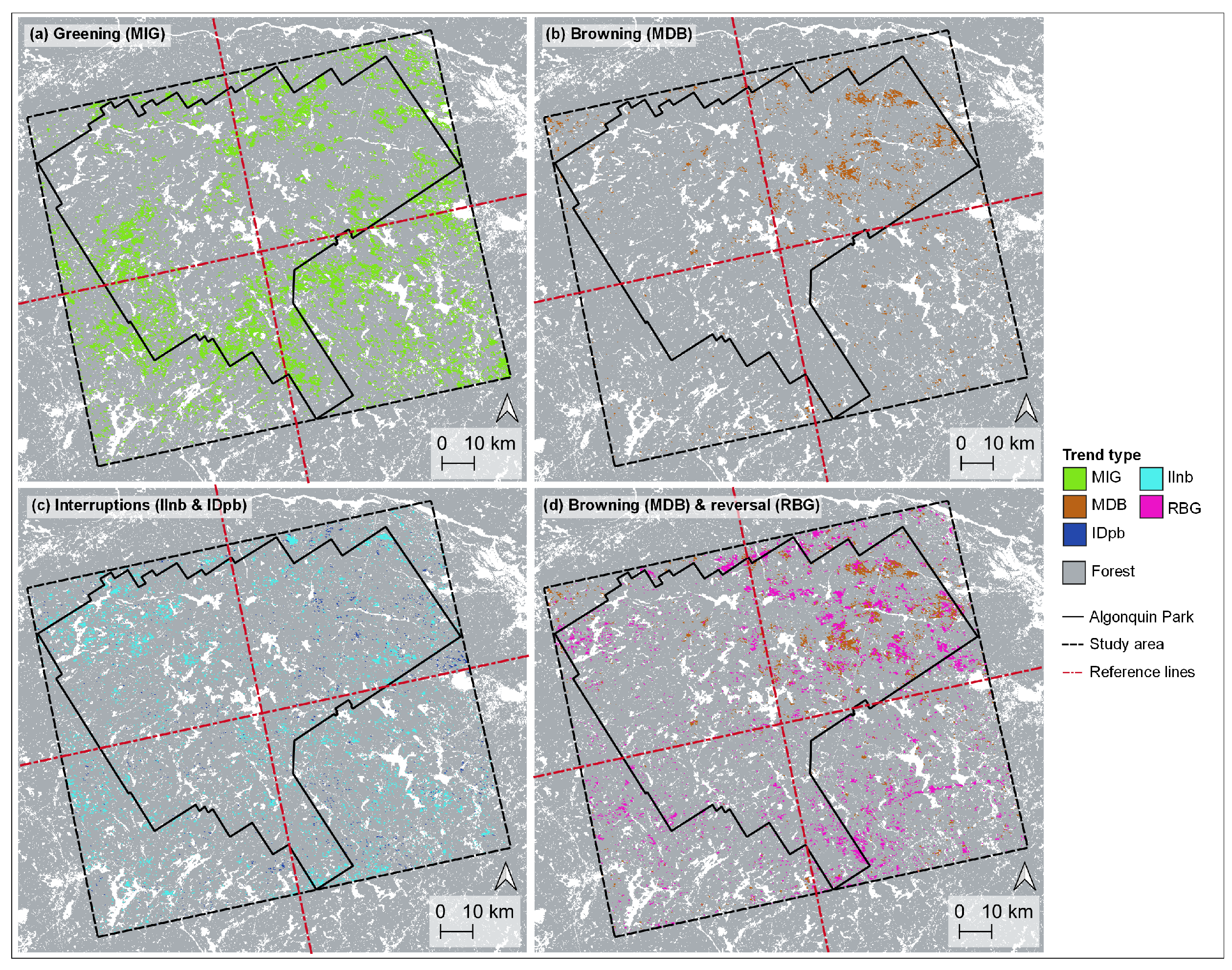
Geographic distribution of trends in Algonquin Park and the surrounding area, which we refer to as the Algonquin Greater Park Ecosystem (AGPE). All maps show trends that were derived from the output of bfastclassify. Compared to greening trends (MIG) which occurred throughout the AGPE (a), browning trends (MDB) mostly occurred in the NE quadrant (b). Most increasing trends with negative breaks (interruptions, IInb) occurred in the NW quadrant (c) while most of the relatively few decreasing trends with positive breaks (interruptions, IDpb) occurred in the NE quadrant (c). Notably, browning to greening reverse trends (RBG) co-occurred with browning trends in the NE quadrant (d). The dashed black line shows the study area footprint (1.5 M ha). The solid black line shows Algonquin Provincial Park’s footprint. The perpendicular dashed lines divide the study area into four quadrants (northwest, NW; northeast, NE; southwest, SW; and southeast, SE) to ease the description of the results. Map projection across all figures is NAD83 Statistics Canada Lambert, EPSG: 3347.
Figure A6.
Geographic distribution of trends in Algonquin Park and the surrounding area, which we refer to as the Algonquin Greater Park Ecosystem (AGPE). All maps show trends that were derived from the output of bfastclassify. Compared to greening trends (MIG) which occurred throughout the AGPE (a), browning trends (MDB) mostly occurred in the NE quadrant (b). Most increasing trends with negative breaks (interruptions, IInb) occurred in the NW quadrant (c) while most of the relatively few decreasing trends with positive breaks (interruptions, IDpb) occurred in the NE quadrant (c). Notably, browning to greening reverse trends (RBG) co-occurred with browning trends in the NE quadrant (d). The dashed black line shows the study area footprint (1.5 M ha). The solid black line shows Algonquin Provincial Park’s footprint. The perpendicular dashed lines divide the study area into four quadrants (northwest, NW; northeast, NE; southwest, SW; and southeast, SE) to ease the description of the results. Map projection across all figures is NAD83 Statistics Canada Lambert, EPSG: 3347.
![Remotesensing 16 02919 g0a6]()


