A Small Maritime Target Detection Method Using Nonlinear Dimensionality Reduction and Feature Sample Distance

Abstract

Addressing the challenge of radar detection of small targets under sea clutter, target detection methods based on a three-dimensional feature space have shown effectiveness. However, their application has revealed several problems, including high dependency on linear relationships between features for dimensionality reduction, unclear reduction objectives, and spatial divergence of target samples, which limit detection performance. To mitigate these challenges, we constructed a feature density distance metric employing copula functions to quantitatively describe the classification capability of multidimensional features to distinguish targets from sea clutter. On the basis of this, a lightweight nonlinear dimensionality reduction network utilizing a self-attention mechanism was developed, optimally re-expressing multidimensional features into a three-dimensional feature space. Additionally, a concave hull classifier using feature sample distance was proposed to mitigate the negative impact of target sample divergence in the feature space. Furthermore, multivariate autoregressive prediction was used to optimize features, reducing erroneous decisions caused by anomalous feature samples. Experimental results using the measured data from the SDRDSP public dataset demonstrated that the proposed detection method achieved a detection probability more than 4% higher than comparative methods under Sea State 5, was less affected by false alarm rates, and exhibited superior detection performance under different false alarm probabilities from 10⁻³ to 10⁻¹.

1. Introduction

Radar detection of small targets such as boats, icebergs, and frogmen under sea clutter remains a formidable challenge [1,2]. Due to the diversity of small target types and the overlap of their echoes with sea clutter in the frequency domain, traditional MTI and MTD methods are limited in effectiveness and fail to accurately discriminate targets on the basis of a single detection statistic. In such scenarios, extracting and combining various significant features from radar echoes is considered an effective detection approach.

Unlike adaptive model-based detection [3,4,5,6,7], features typically represent certain statistical information extracted from radar echoes in an intuitive or empirical manner and possess certain capabilities to classify targets and sea clutter. To date, dozens of explicit, interpretable empirical features extracted from the time, frequency, and transform domains [8,9,10,11,12], as well as many implicit, uninterpretable machine features [13,14], have been applied to radar target detection.

Different features are suitable for different scenarios [8,9], and their complementarity forms the basis for robust and well-performing feature-based detectors [15]. Thus, multi-feature-based target detection is a strategy for enhancing detection performance. Common multi-feature target detection methods typically construct a multi-dimensional feature space through experience, selecting various features and training specific classifiers. These classifiers include K-nearest neighbors (KNN) [16], support vector machines (SVM) [17,18], convex hull learning algorithms [8], concave hull learning algorithms [19,20], decision tree algorithms [21], and implicit neural networks [22,23], forming effective detectors. Given the necessity for radar to perform target detection under various environmental conditions, feature-based target detection often translates into an outlier detection problem [24]. When more than three types of features are used, the suitability of algorithms based on convex or concave hull learning in the feature space may diminish. Additionally, as the number of features increases, the curse of dimensionality becomes a significant problem. To address this issue, feature dimensionality reduction techniques, such as Principal Component Analysis (PCA) [25], Linear Discriminant Analysis (LDA) [26], and feature compression [15], can be employed. Although these methods can utilize correlations between features, these correlations are limited to linear relationships, such as Pearson correlation coefficients. Furthermore, the dimensionality reduction process of these methods is linear, which does not align with the nonlinear relationships between different features in practical scenarios, thus increasing system error and reducing detection performance. Additionally, during the detection phase, these methods require comparing the positions of target samples and decision regions in a three-dimensional feature space, where target samples have high divergence, making stable detection difficult. Moreover, feature extraction is also affected by anomalies such as sea spikes, resulting in anomalous samples.

To address these problems, this paper first analyzes the nonlinear relationships between 11 common radar echo features. On the basis of the analysis results, a small maritime target detection method using nonlinear dimensionality reduction and feature sample distance is proposed. This method first defines a feature density distance and employs the copula function to reduce computational difficulty. A lightweight nonlinear dimensionality reduction network based on the self-attention mechanism was designed to optimally re-express multidimensional features into a three-dimensional feature space with optimal joint classification capability. Furthermore, a concave hull classifier using the feature sample distance is proposed, leveraging the sample distance between new features and the convergence of clutter samples in the feature space to enhance detection performance. Finally, multivariate autoregressive prediction was used to optimize features, reducing erroneous decisions caused by anomalous feature samples. Validation with real data from the SDRDSP public radar dataset demonstrated that the proposed method outperforms other feature-based target detection methods.

The remainder of this paper is organized as follows: Section 2 briefly introduces the public radar dataset and the 11 significant features used. Section 3 analyzes the nonlinear correlations of the features and proposes a small maritime target detection method using nonlinear dimensionality reduction and feature sample distance. Section 4 validates the proposed method with real data and discusses it in comparison with five feature-based target detection methods. Finally, Section 5 concludes the paper.

2. Datasets and Features

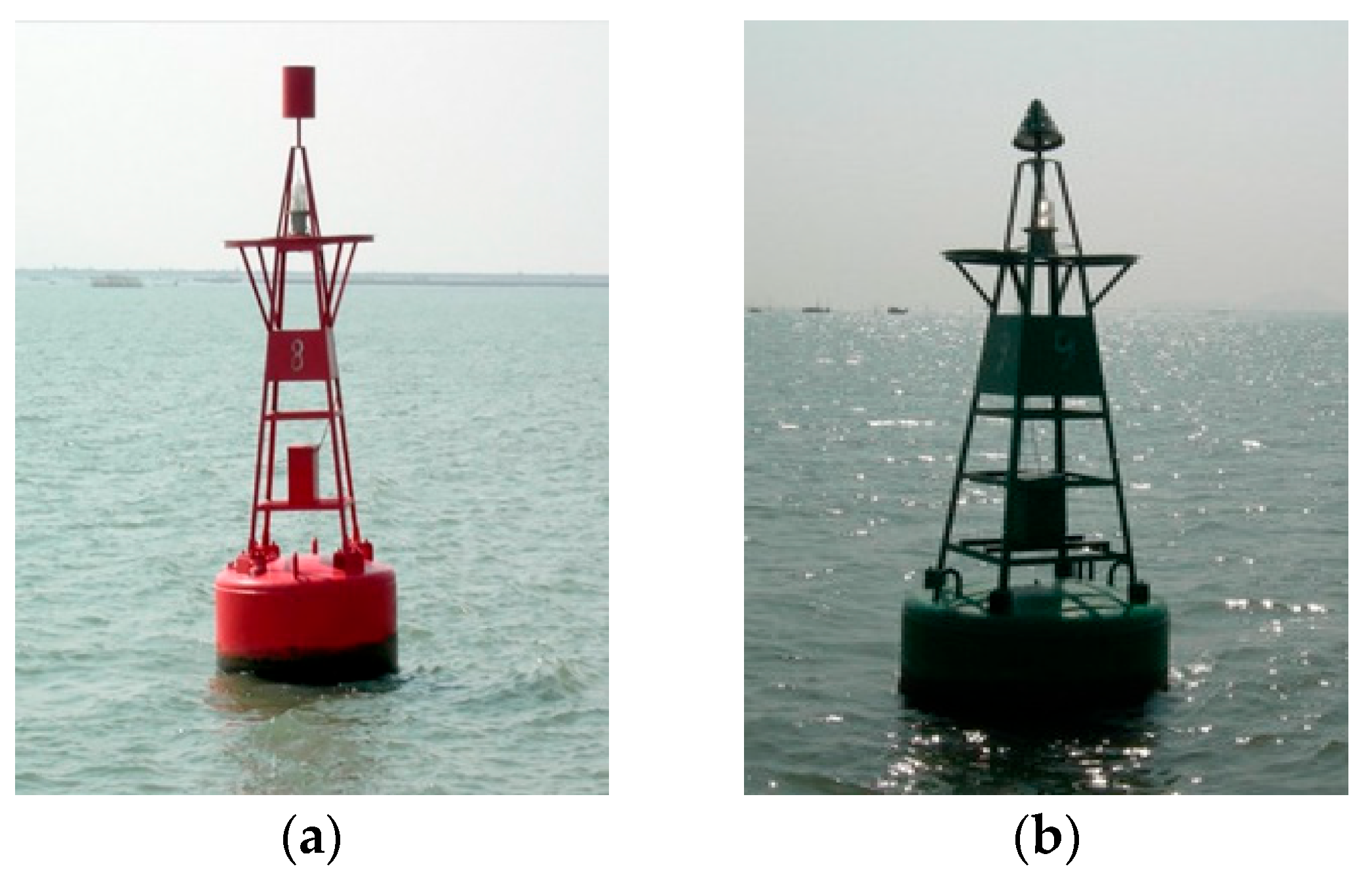
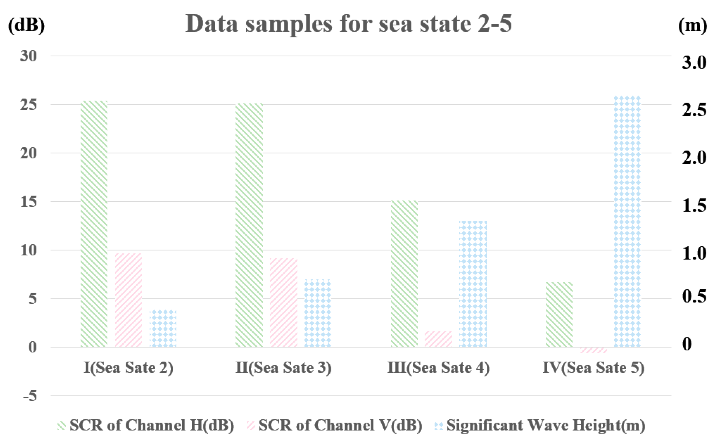
2.1. Description of the Measured Experimental Data

In this study, the radar measurement data utilized originate from the self-measured dataset available within the “Radar Marine Detection Data Sharing Program (SDRDSP)”, hosted by the Naval Aeronautical University [27,28]. This dataset stands as one of the public datasets commonly employed for maritime target detection research in contemporary studies.

Its objective is to conduct phased and batched marine exploration experiments using X-band solid-state phased-array radar. These experiments involve data collection on targets and sea clutter under various sea states. Simultaneously, the dataset gathers authentic marine meteorological and hydrological data, along with the actual positions and trajectories of targets. The radar is located on a tall tower on the coast of Yantai, China, with a peak transmission power of 100 W.

Table 1. The parameters of the SDRDSP dataset.

Database	SDRDSP
Carrier frequency	9.3~9.5 GHz
PRF	2000 Hz
Range resolution	6 m
Polarization	HH/HV/VH/VV
Operating mode	Staring
Band	X
Test target	Two light buoys
Average SCR	−2~25.1 dB
Radial velocity	−0.8~0.9 m/s

lists important information about this dataset. Relevant data can be obtained from the Journal of Radars website (https://radars.ac.cn/web/data/getData?dataType=DatasetofRadarDetectingSea, accessed on 3 July 2024).

The targets were set as two light buoys, located 2.97 and 3.19 nautical miles from the radar, anchored and floating on the sea surface, as shown in Figure 1. The data length is 2¹⁷ points, with 1000 distance sampling points. The experimental data include sea states ranging from level 2 to 5, with average signal-to-clutter ratios (SCRs) and effective wave heights under four sea states as shown in Figure 2.

2.2. Description of the Significant Features

Taking maritime radar as an example, assume that it transmits a series of coherent pulses on each transmit-receive channel and receives complex time series for each range cell. The problem of radar target detection under sea clutter can be transformed into the following binary hypothesis testing problem [29], as shown in (1)

$$\begin{array}{cc}\begin{array}{l}{H}_0\left\{\begin{array}{l}x(n)=c(n),\\ x_p(n)=c_p(n),\end{array}\right.\\ H_1\left\{\begin{array}{l}x(n)=s(n)+c(n),\\ x_p(n)=c_p(n),\end{array}\right.\end{array}& \begin{array}{l}n=1,2,\dots ,N\\ p=1,2,\dots ,K\\ n=1,2,\dots ,N\\ p=1,2,\dots ,K\end{array}\end{array}$$

(1)

where $N$ represents the length of the received complex time series, $K$ denotes the number of reference cells (RC), and $x(n)$ and $x_p(n)$ are the radar echo time series received at the cell under test (CUT) and RCs, respectively. $c(n)$ and $c_p(n)$ represent the sea clutter time series at the CUT and RCs, while $s(n)$ is the unknown radar echo. The null hypothesis H₀ and the alternative hypothesis H₁ correspond to the scenarios where only sea clutter is present at the CUT or both sea clutter and a target are present, respectively.

Calculating the features of radar echoes using the time series $x(n)$ and $x_p(n)$ and employing a classifier to make decisions regarding the detection problem is known as the feature-based target detection method. This paper utilizes the measured datasets from Section 2.1 to extract 11 significant radar echo features, which are briefly introduced below according to their respective transform domains.

2.2.1. Features in the Time Domain

• Relative Average Amplitude [8]: RAA is defined as the ratio of the average amplitude of the CUT to that of the RCs, and it is used to measure the amplitude difference between the CUT and the RCs, as shown in (2):

  $$RAA\left(x;x_p\right)={\displaystyle \frac{\overline{A}\left(x\right)}{\frac{1}{K}{\displaystyle \sum _{p=1}^K\overline{A}\left(x_p\right)}}}$$

  (2)

  $$\overline{A}\left(x\right)={\displaystyle \frac{1}{N}}{\displaystyle \sum _{n=1}^N\left|x\left(n\right)\right|}$$

  (3)

  where $x$ and $x_p$ are abbreviations of $x(n)$ and $x_p(n)$.
• Time Domain Entropy Mean [30]: TEM is defined as the average entropy of the echo at the CUT. Due to the differing fluctuations in the echoes, it reflects the level of disorder in the waveforms of the target and sea clutter signals. Using a $W$ wide rectangular window and an S wide step, slide the echo signal $x$ at the CUT to obtain $⌈(N-W+1)/S⌉$ time-domain short sequences $\left\{s_i\right\}$ with a length of $W$. The calculation is shown in (7).

  $$\begin{array}{cc}\begin{array}{ll}{s}_i& =[s_i(1),\dots ,s_i(W)]\\ & =[x(1+(i-1)S),\dots ,x(1+(i-1)S+W-1)]\end{array}& ,i=1,2,\dots ,⌈{\displaystyle \frac{N-W+1}{S}}⌉\end{array}$$

  (4)

  $$TE(i)=-{\displaystyle \sum _{w=1}^W{p}_i\left(w\right){\log }_2{p}_i\left(w\right)}$$

  (5)

  $$p_i\left(w\right)={\displaystyle \frac{s_i(w)}{{\displaystyle \sum _{w=1}^W{s}_i(w)}}}$$

  (6)

  $$TEM(x)={\displaystyle \frac{1}{⌈(N-W+1)/S⌉}}{\displaystyle \sum _{i=1}^{⌈(N-W+1)/S⌉}TE(i)}$$

  (7)

  where $⌈·⌉$ represents rounding up, and $TE(i)$ represents the time-domain entropy value of the i-th short sequence $s_i$.
• Relative Peak Height: RPH is defined as the ratio of the peak amplitude of the pulse echo at the CUT to the average amplitude of adjacent pulses. This can be used to reflect the differences in energy proportion and peak fluctuations between the target and sea clutter echoes, as shown in (8):

  $$RPH\left(x\right)={\displaystyle \frac{MAX\left(x\right)}{\frac{1}{\#\Delta }{\displaystyle {\sum }_{n\in n^{\max }+\Delta }(A\left(x_{\Delta }\right))}}}$$

  (8)

  $$\Delta =[-{\tau }_1,-{\tau }_2]\cup [{\tau }_2,{\tau }_1]$$

  (9)

  where $\#\Delta$ represents the number of units in set $\Delta$, while ${\tau }_1$ and ${\tau }_2$ collectively specify the pulse range used in the ratio calculation.

2.2.2. Features in the Frequency Domain

• Relative Doppler Peak Height [8]: RDPH is defined as the ratio of the Doppler peak at the CUT to the average Doppler peak of the RCs. This can illustrate the differences in the proportion of energy at frequency peaks and the degree of abrupt changes between the two types of echoes. The calculation is shown in (10):

  $$RDPH\left(x;x_p\right)={\displaystyle \frac{DPH\left(x\right)}{\frac{1}{K}{\displaystyle \sum _{p=1}^{K}DPH\left(x_p\right)}}}$$

  (10)

  $$DPH\left(x\right)={\displaystyle \frac{DAS\left(f_{\mathrm{d}}^{\max };x\right)}{\frac{1}{\#\gamma }{\displaystyle \sum _{f_{\mathrm{d}}\in f_{\mathrm{d}}^{\max }\left(x\right)+\gamma }DAS\left(f_{\mathrm{d}};x\right)}}}$$

  (11)

  $$DAS\left(f_{\mathrm{d}};x\right)={\displaystyle \frac{1}{\sqrt{N}}}\left|{\displaystyle \sum _{n=1}^{N}x(n)\exp (-2\pi f_{\mathrm{d}}n{T}_{\mathrm{r}})}\right|$$

  (12)

  $$f_{\mathrm{d}}^{\max }\left(x\right)=\underset{f_{\mathrm{d}}}{\arg \max }\left\{DAS\left(f_{\mathrm{d}};x\right)\right\}$$

  (13)

  $$\gamma =\left[-{\phi }_1,{\phi }_2\right]\cup \left[{\phi }_2,{\phi }_1\right]$$

  (14)

  where $T_{\mathrm{r}}$ represents the pulse repetition period and $f_{\mathrm{d}}$ is the Doppler frequency. $\#\gamma$ indicates the number of channels in set $\gamma$, and ${\phi }_1$ and ${\phi }_2$ together define the range of Doppler channels involved in the ratio calculation.
• Relative Vector Entropy [8]: RVE is defined as the ratio of the information entropy between the CUT and the RCs, which reflects the level of disorder in the signal waveforms. The calculation is shown in (15).

  $$RVE\left(x;x_p\right)={\displaystyle \frac{VE\left(x\right)}{\frac{1}{K}{\displaystyle \sum _{p=1}^{K}VE\left(x_p\right)}}}$$

  (15)

  $$VE\left(x\right)=-{\displaystyle \sum _{f_{\mathrm{d}}}\overline{DAS}\left(f_{\mathrm{d}}|x\right){\log }_2(\overline{DAS}\left(f_{\mathrm{d}}|x\right))}$$

  (16)

  $$\overline{DAS}\left(f_{\mathrm{d}}|x\right)=DAS\left(f_{\mathrm{d}}|x\right)/{\displaystyle \sum _{f_{\mathrm{d}}}DAS\left(f_{\mathrm{d}}|x\right)}$$

  (17)
• Second Moment of Frequency Domain Entropy: SOFE is defined as the variance of the entropy in the frequency domain at the CUT, reflecting the dispersion of entropy values across the series. The calculation is shown in (21).

Calculate the Fourier transform of the time-domain short sequence $\left\{s_i\right\}$ obtained from (4) to obtain the corresponding frequency-domain sequence $\left\{f_i\right\}$:

$$f_i=[f_i(1),\dots ,f_i(W)],i=1,2,\dots ,⌈{\displaystyle \frac{N-W+1}{S}}⌉$$

(18)

$$FE(i)=-{\displaystyle \sum _{w=1}^W{p}_{\mathrm{f},i}\left(w\right){\log }_2{p}_{\mathrm{f},i}\left(w\right)}$$

(19)

$$p_{\mathrm{f},i}\left(w\right)={\displaystyle \frac{f_i(w)}{{\displaystyle \sum _{w=1}^W{f}_i(w)}}}$$

(20)

$$SOFE(x)=\overline{{(FE(i)-\overline{FE})}^2}$$

(21)

where $FE(i)$ represents the frequency domain entropy of the i-th short sequence $s_i$, and $\overline{·}$ denotes the mean value.

2.2.3. Features in the Time-Frequency Domain

• Ridge Integration [9]: RI is defined as the cumulative value of time-frequency ridges in the spectrum of the CUT, reflecting the energy strength of the time-frequency ridges. The calculation is shown in (22):

  $$\begin{array}{l}RI\left(x;x_p\right)=\\ {\displaystyle \sum _{n=1}^{N}NTFD\left(n,\underset{f_{\mathrm{d}}}{\arg \max }\left\{NTFD\left(n,f_{\mathrm{d}}|x;x_p\right)\right\}|x;x_p\right)}\end{array}$$

  (22)

  $$\begin{array}{l}NTFD\left(n,f_{\mathrm{d}}|x;x_p\right)=\\ {\displaystyle \frac{SPWVD(n,f_{\mathrm{d}}|x)-\frac{1}{K}{\displaystyle \sum _{p=1}^{K}SPWVD(n,f_{\mathrm{d}}|x_p)}}{\sqrt{\frac{1}{K-1}{\displaystyle \sum _{p=1}^K{(SPWVD(n,f_{\mathrm{d}}|x_p)-\frac{1}{K}{\displaystyle \sum _{p=1}^{K}SPWVD(n,f_{\mathrm{d}}|x_p)})}^2}}}}\end{array}$$

  (23)

  where $SPWVD(n,f_{\mathrm{d}}|x)$ represents the smoothed pseudo-Wigner–Ville distribution of the received sequence $x$ at the CUT.
• Maximal Size of Connected Regions [9]: MS is defined as the maximum number of threshold-exceeding points in each connected region in the binary time-frequency spectrum. The calculation is shown in (24):

  $$MS(x;x_p)=\max \{\mathrm{num}({\Gamma }_1),\dots ,\mathrm{num}({\Gamma }_C)\}$$

  (24)

  where ${\Gamma }_C$ represents one connected region in the set of connected regions $\mathbf{\Gamma }=[{\Gamma }_1,\dots ,{\Gamma }_C]$, and $\mathrm{num}({\Gamma }_C)$ is the number of time-frequency ridge points within the connected region ${\Gamma }_C$.
• Number of Connected Regions [9]: NR is defined as the count of connected regions in the binary time-frequency spectrum, indicating the degree of dispersion of time-frequency ridge energy. The calculation is shown in (25).

  $$NR\left(x;x_p\right)=C$$

  (25)

2.2.4. Features in the Time-Frequency Ridge Transform Domain

• Ridges Radon Transform Maximum Value [31]: RRT-MV is defined as the maximum value in the time-frequency ridge transform domain. The calculation is shown in (26):

  $$RRT\text{-}MV(x;x_p)=\max \left\{R\left(\rho ,\theta |x;x_p\right)\right\}$$

  (26)

  $$\begin{array}{l}R\left(\rho ,\theta |x;x_p\right)=\\ {\displaystyle \iint Ridge\left(n,f_{\mathrm{d}}|x;x_p\right)}\delta \left(\rho -n\cos \theta -f_{\mathrm{d}}\sin \theta \right)dnd{f}_{\mathrm{d}}\end{array}$$

  (27)

  $$\begin{array}{l}Ridge\left(n,f_{\mathrm{d}}|x;x_p\right)\\ =\left\{\begin{array}{c}1,f_{\mathrm{d}}=\underset{f_{\mathrm{d}}}{\arg \max }\left\{NTFD\left(n,f_{\mathrm{d}}|x;x_p\right)\right\}\\ 0,f_{\mathrm{d}}\ne \underset{f_{\mathrm{d}}}{\arg \max }\left\{NTFD\left(n,f_{\mathrm{d}}|x;x_p\right)\right\}\end{array}\right.\end{array}$$

  (28)

  where $Ridge\left(n,f_{\mathrm{d}}|x;x_p\right)$ refers to the time-frequency ridge image of $x$, $\theta$ is the angle parameter, $\rho$ is the distance parameter, and $\delta (·)$ represents the Dirac function.
• Ridges Radon Transform Band Width [31]: RRT-BW reflects the dispersal of time-frequency ridge sequences along the radial coordinate axis $\rho$ and the concentration of ridge energy. The calculation is shown in (29):

  $$\begin{array}{l}RRT\text{-}BW(x;x_p)=\\ \underset{\xi }{\mathrm{argmin}}\{COEFF*P<{\displaystyle \sum _{\rho ={\rho }_{\mathrm{MAX}}-\xi /2}^{{\rho }_{\mathrm{MAX}}-\xi /2}R(\rho ,{\theta }_{\mathrm{MAX}}|x;x_p)}\}\end{array}$$

  (29)

  where $({\rho }_{\mathrm{MAX}},{\theta }_{\mathrm{MAX}})$ represents the coordinates of the peak point $R(\rho ,\theta |x;x_p)$, $P$ represents the number of coherent pulses, and $COEFF$ is the preset bandwidth coefficient.

3. A Small Maritime Target Detection Method Using Nonlinear Dimensionality Reduction and Feature Sample Distance

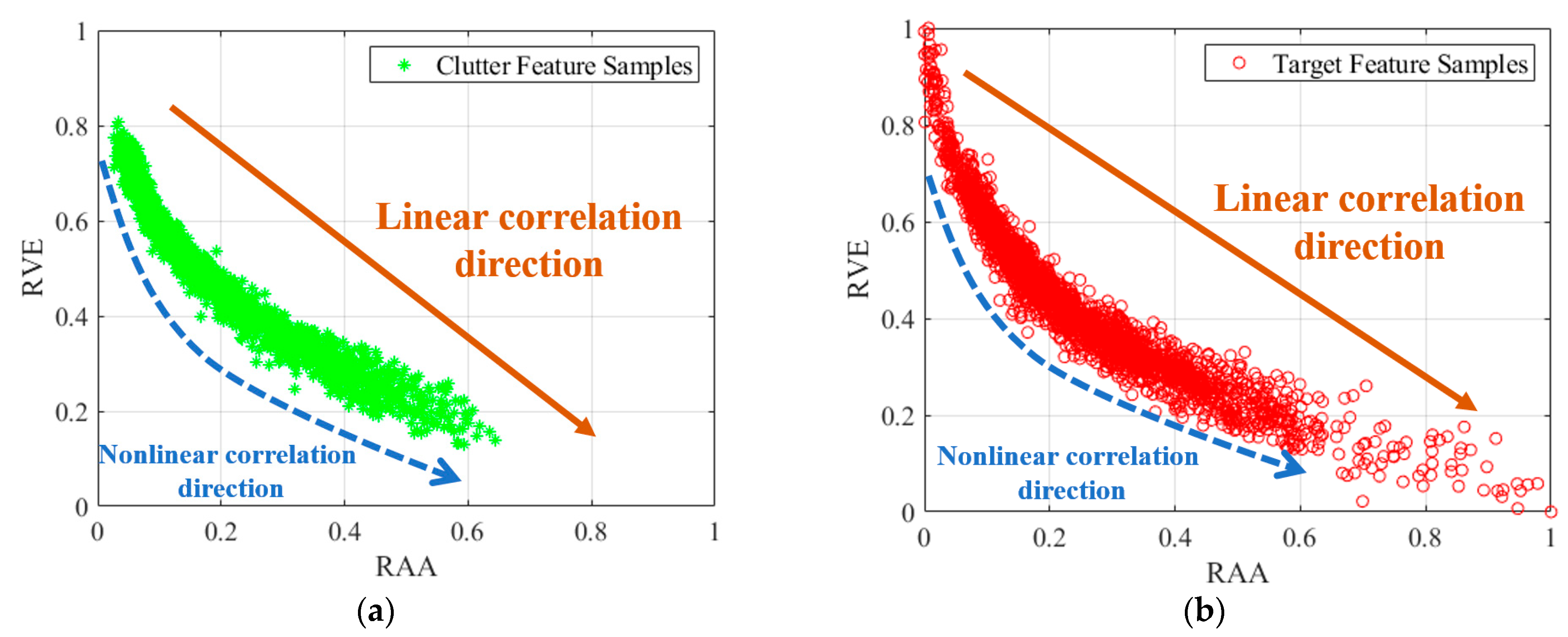
3.1. Analysis of the Correlations between Features

In this subsection, we use data under Sea State 5 in the SDRDSP measured dataset to extract the 11 features introduced in Section 2.2 from both target and clutter cells. After normalization, the amplitude distribution characteristics are analyzed, and the results are shown in Figure 3. Before conducting the correlation analysis between features, we first need to quantitatively measure the classification ability of individual features for sea clutter and targets. Here, we introduce the Bhattacharyya distance (BD), defined as follows in (30):

$$D_{\mathrm{b}}(p,q)=-ln({\displaystyle {\int }_x\sqrt{p(g)q(g)}})$$

(30)

where $p$ and $q$ are the probability density functions (PDF) of the same feature under different classes of data and $g$ represents the range of a single feature, with values between [0, 1]. The physical meaning is that the BD represents the proportion of the overlapping part of the two PDFs to the total, taking the logarithm and the negative value. The larger the overlapping area of the two PDFs, the smaller the BD, and the harder it is to distinguish between the two categories, and vice versa. Therefore, we can calculate the BD for the 11 features with respect to sea clutter and targets, as shown in Figure 4.

The probability density of a feature can be viewed as the sample distribution in a one-dimensional feature space. From Figure 3, it can be seen that the feature samples extracted from sea clutter cells tend to be highly concentrated around the mean of that feature, which is visually reflected as a smaller variance. By contrast, the feature samples extracted from target cells often exhibit a larger variance and are more widely distributed across the entire range. Most features show a high degree of overlap between the two types of cells, indicating that under such conditions, their classification ability is limited. By closely observing the portions of the target cells outside the overlapping area, it can be found that they typically have a longer leading or trailing tail compared with the clutter cells. This suggests that, compared with clutter, the feature samples of targets usually have a greater dispersion in the feature space, often diverging toward the value range opposite to the clutter sample aggregation area. For instance, clutter samples of RAA are concentrated in the low-value region, while target samples diverge and tail towards the high-value region. This characteristic provides effective support for the feature sample distance-based algorithm proposed later. According to the BD in Figure 4, it can be inferred that the overlap of PDFs corresponding to samples from the two types of cells varies significantly among different features under the same conditions. RI, RDPH, and RAA exhibit strong discriminative effects when used alone, whereas SOFE, MS, and NR have weaker distinguishing capabilities, mainly because the targets under these data conditions are slow-moving floating targets. This indicates that relying on a single feature for detection has limited performance.

Current feature-based target detection methods tend to use Pearson correlation coefficients to describe the linear correlation when depicting the relationships between different features. However, in most scenarios, features often exhibit nonlinear relationships rather than linear ones. Figure 5 and Figure 6 illustrate the relative positional relationship of feature samples of RAA and RVE as an example.

As shown in the Figures, the feature samples of both target cells and sea clutter cells do not conform to a linear relationship; their distribution is more akin to a nonlinear relationship resembling a polynomial function. As the sea state increases, this nonlinear relationship does not disappear; rather, the divergence of the target samples intensifies.

Using polynomial functions to test the correlations among three features in a three-dimensional feature space yields the following Figure 7. It can be observed that there is a clear nonlinear relationship among the three features, which can largely be described by polynomial functions.

In summary, we can conclude that if linear dimensionality reduction techniques such as PCA and LDA are forcibly used in the feature re-expression process, the direction of maximum variance that can be found will be the one under linear conditions rather than the true distribution of maximum variance among the samples. This will inevitably lead to a loss of information and limited detection performance. Therefore, it is crucial to establish a nonlinear feature re-expression method.

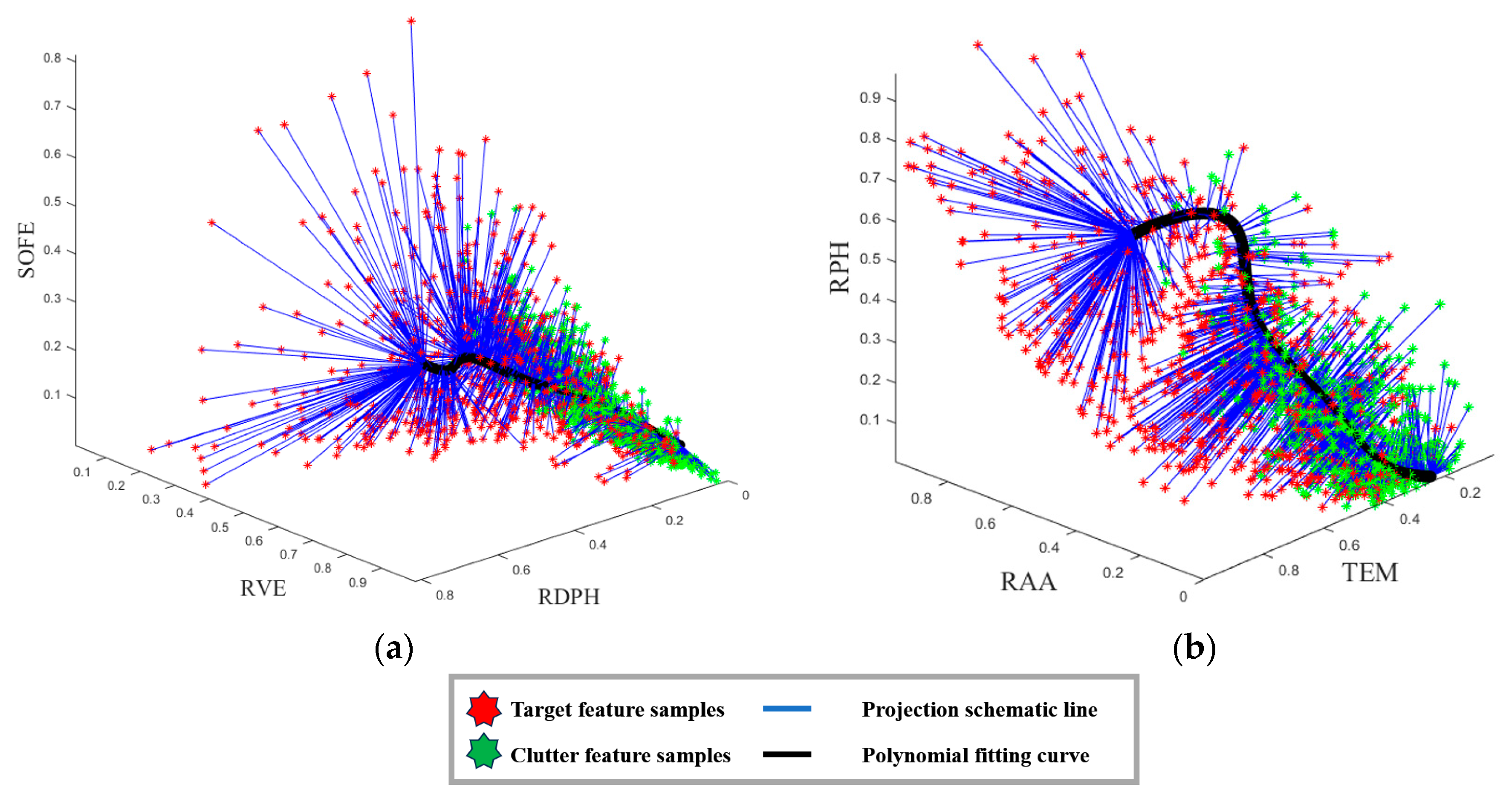
3.2. Nonlinear Dimensionality Reduction Method Using a Feature Density Distance Metric

3.2.1. Feature Density Distance

To construct a nonlinear dimensionality reduction method, it is first necessary to clarify the ultimate goal of feature dimensionality reduction, specifically how to define a metric to describe the classification capability of features in a multidimensional feature space. The BD is a commonly used metric for measuring classification capability, but it has two major problems that make it unsuitable for this dimensionality reduction method: the calculation is too difficult, and the measurement standard is too singular.

Firstly, the computational difficulty: Calculating the BD requires computing the joint PDF among multidimensional features. This step is typically achieved by differentiating the joint distribution function or directly using kernel estimation methods. The former involves multivariate differentiation operations, which have high computational complexity, while the latter largely ignores the correlations between features and also typically has high computational difficulty. In some literature [15], the BD is computed using a derived formula under the conditions of multivariate Gaussian distribution. However, as shown in previous Figure 3, the distribution types of features mostly do not conform to Gaussian distribution, significantly affecting performance. Secondly, the singular measurement standard: The BD uses the proportion of the overlapping area of the joint PDFs of sea clutter and target in the overall distribution as a metric, but it ignores the characterization of the overlapping part. For instance, under the same overlapping proportion, it cannot quantitatively describe the size or density of the overlapping region, which is crucial in the implementation of detection algorithms.

Therefore, we propose a feature density distance to describe the classification capability of features in a multidimensional feature space. The definition is as follows in (31).

$$D_{\mathrm{d}}(p,q)=w(p,q)+0.5·\eta (p,q)·(1-w(p,q))$$

(31)

$$w(p,q)=1-{\displaystyle \frac{2}{1+{\mathrm{e}}^{-5(\sqrt{{\lambda }_{\mathrm{overlap}}}-1)}}}=1-{\displaystyle \frac{2}{1+{\mathrm{e}}^{-5(\sqrt{{\displaystyle {\int }_x\sqrt{p(g)q(g)}}}-1)}}}$$

(32)

$$\eta (p,q)=2(1-{\displaystyle \frac{1}{1+{\mathrm{e}}^{-10({\lambda }_{\mathrm{density}}-1)}}})$$

(33)

$$\begin{array}{cc}{\lambda }_{\mathrm{density}}& =\sqrt[d]{V_{-3\mathrm{dB}}(p(g),q(g))/V(p(g),q(g))}\\ & =\sqrt[d]{\#(\sqrt{p(g),q(g)}>0.707·\max (\sqrt{p(g),q(g)}))/\#(\sqrt{p(g),q(g)})}\end{array}$$

(34)

where $p$ and $q$ are the probability density functions of the same feature under different classes of data. 0.5 is a tuning parameter used to balance the importance of $w$ and $\eta$. It is empirically selected as the optimal ratio based on test results. $g$ is the feature matrix with a range of ${[0, 1]}^d$, representing the range of multidimensional features. $d$ is the dimensionality of the feature space. $V_{-3\mathrm{dB}}$ represents: the number of elements that are greater than −3 dB (0.707 times) of the maximum value in the matrix. $V$ represents the total number of elements in a multidimensional matrix. $\#(·)$ is the number of elements in the multidimensional matrix. $\mathrm{e}$ is the natural logarithm.

The definition of feature density distance can be understood using Figure 8. Similar to the BD, the $w$ component of the feature density distance is an overlap parameter used to represent the degree of overlap between the joint PDFs. Unlike the BD, which uses the logarithmic function to make a meaningless and infinite range fine division of low overlap areas, the definition of $w$ can focus more on high overlap areas, providing more feedback for the reduction of overlap proportion and better describing the classification capability brought by the degree of overlap. Using a 2-dimensional feature space as an example in Figure 9, the $\eta$ component of the feature density distance is a density parameter used to represent the density of the overlapping part of the joint PDFs of the two classes. It quantifies the degree of sample aggregation in the overlap area by measuring the volume of the multidimensional feature space occupied by the peak value of the overlap part falling to −3 dB. The stronger the aggregation, the smaller the ${\lambda }_{\mathrm{density}}$, the larger the $\eta$, and the greater the feature density distance. As shown in Figure 10, the significance of the $\eta$ component lies in its use with classifiers in the feature space, such as a concave hull-based target detector. During the construction of the concave hull, the false alarm control vertices in the overlapping area will be removed. The more concentrated the sample density, the more likely the target samples are to detach from the concave hull and be correctly detected.

In the process of calculating the feature density distance, there is a challenge similar to that of the BD, which is the calculation of the joint PDF. Here, we introduce the copula function. According to Sklar’s theorem [32], the copula function can combine the marginal distribution functions of two features into a joint PDF. Furthermore, by constructing a Copula vine, we can calculate the multidimensional joint PDF. This process involves only pairwise joint operations between features, avoiding differential calculations and significantly reducing computational complexity. The calculation process is shown in (35).

$$\begin{array}{l}p(g)=\\ {\displaystyle \prod _{k=1}^d{f}_k(g_k)}{\displaystyle \prod _{i=1}^{d-1}{\displaystyle \prod _{j=i+1}^d{c}_{i,j|i+1,i+2,\dots ,j-1}(F_{i|i+1,i+2,\dots ,j-1}(g_i|g_{i+1},g_{i+2},\dots ,g_{j-1}),F_{j|i+1,i+2,\dots ,j-1}(g_j|g_{i+1},g_{i+2},\dots ,g_{j-1}))}}\end{array}$$

(35)

$$\begin{array}{cc}\hfill c_{i,j|\mathrm{condition}}(F_{i|\mathrm{condition}},F_{j|\mathrm{condition}})& ={\displaystyle \frac{1}{\sqrt{\left|\Sigma \right|}}}{\mathrm{e}}^{(-{\displaystyle \frac{1}{2}}(z^{\mathrm{T}}({\Sigma }^{-1}-I)z))}\hfill \\ & ={\displaystyle \frac{1}{\sqrt{\left|\Sigma \right|}}}{\mathrm{e}}^{(-{\displaystyle \frac{1}{2}}({\Phi }^{-1}(F_{i|\mathrm{condition}}),{\Phi }^{-1}(F_{j|\mathrm{condition}}))({\Sigma }^{-1}-I){({\Phi }^{-1}(F_{i|\mathrm{condition}}),{\Phi }^{-1}(F_{j|\mathrm{condition}}))}^{\mathrm{T}})}\hfill \end{array}$$

(36)

where ${\Phi }^{-1}(·)$ is the inverse function of the standard normal distribution, $I$ is a $d\times d$ identity matrix, and $\Sigma$ is the covariance matrix. $c_{i,j|\mathrm{condition}}(·)=c_{i,j|i+1,i+2,\dots ,j-1}(·)$ represents the value of the copula density function for features $i$ and $j$ given feature $\{i+1, i+2, \dots , j-1\}$. $F_{i|\mathrm{condition}}(·)=F_{i|i+1,i+2,\dots ,j-1}(·)$ denotes the marginal distribution function of feature $g_i$ given feature $\{g_{i+1}, g_{i+2}, \dots , g_{j-1}\}$.

In summary, the feature density distance $D_{\mathrm{d}}$ can achieve a higher value when the overlap proportion of the two joint PDFs is small and the overlap density is high. By using nonlinear weighting of the two components, their mutual influence is realized. For example, when the overlap proportion is very low, the impact of overlap density is reduced, while when the overlap proportion is very high, the impact of overlap density is automatically amplified. Thus, the problem of nonlinear dimensionality reduction of features becomes how to reduce the feature dimensions while maximizing the feature density distance $D_{\mathrm{d}}$ of the new features.

3.2.2. Nonlinear Dimensionality Reduction Method Using a Lightweight Self-Attention Mechanism Network

On the basis of the analysis in Section 3.1, polynomial functions can be used to fit the nonlinear relationships between features. Thus, low-order polynomials of each feature can be used as an extension of the feature dimensions. Subsequently, the optimal projection matrix can be estimated to achieve dimensionality reduction of the features, ultimately maximizing the feature density distance $D_{\mathrm{d}}$ of the new features. Accordingly, this subsection proposes a relatively lightweight self-attention nonlinear dimensionality reduction network. The self-attention mechanism is a network structure that effectively captures the correlations between each feature and its powers. After capturing the correlation information, dimensionality reduction can be achieved through a linear dimensionality reduction layer, using the negative feature density distance $D_{\mathrm{d}}$ of the new features as the loss function to calculate gradient propagation and achieve optimal dimensionality reduction. Due to the few layers and highly lightweight structure of this dimensionality reduction network, it can effectively avoid high computational complexity while achieving the dimensionality reduction objective. The entire nonlinear dimensionality reduction method based on the feature density distance metric is shown in Figure 11.

3.3. Target Detector Based on Feature Sample Distance

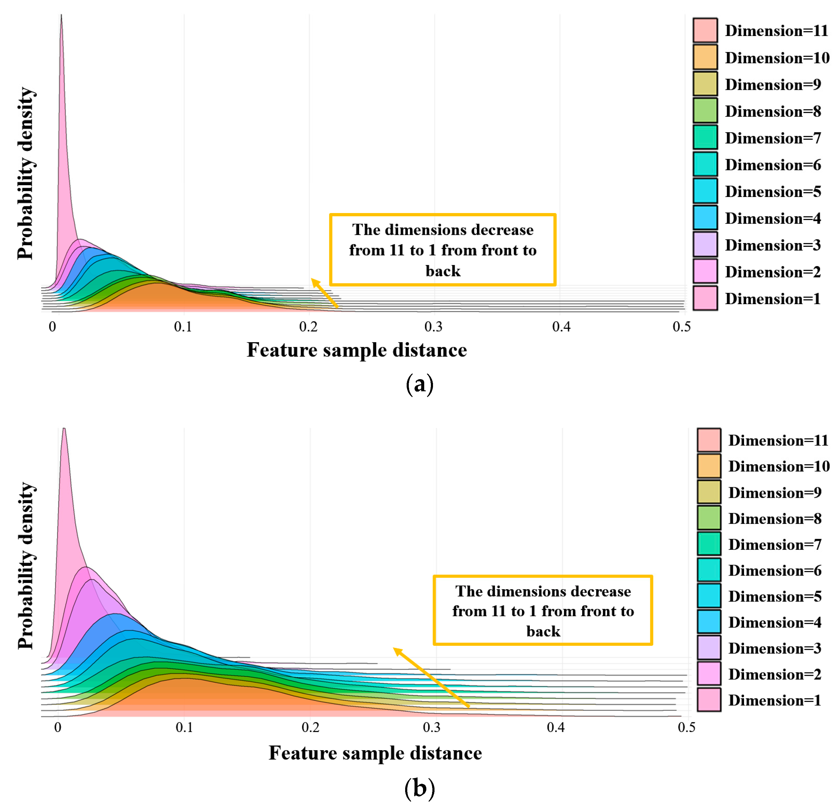
3.3.1. Feature Sample Distance

A multidimensional feature vector can essentially be regarded as the coordinate values of sample points in a multidimensional feature space. As discussed in Section 2.2, the feature sequences of adjacent range cells can essentially be viewed as two time series that simultaneously vary over time. Therefore, the feature sample distance between two adjacent feature samples at the same time can be calculated. In this study, the Euclidean distance between sample points is defined as the feature sample distance. The following (37) represents the feature sample distance between two fixed adjacent feature sample points $g_1$ and $g_2$ in a feature space of dimension M:

$$D_{\mathrm{sample}}(g_1(g_{1,1}, g_{1,2}, \dots , g_{1,M}), g_2(g_{2,1}, g_{2,2}, \dots , g_{2,M}))=\sqrt{{(g_{1,1}-g_{2,1})}^2+{(g_{1,2}-g_{2,2})}^2+\dots +{(g_{1,M}-g_{2,M})}^2}$$

(37)

where $g_{i,m}$ represents the m-th feature used as the coordinate of the feature sample point $g_i$ in the feature space.

The feature sample distance between two fixed feature sample points in a multidimensional space exhibits entirely different distribution patterns depending on the dimensionality of the feature space. Data under Sea State 5 in the SDRDSP measured dataset is used, extracting and normalizing the 11 features introduced in Section 2.2 from both target cells and clutter cells. Two fixed samples from both target and clutter cells are selected to form multidimensional feature spaces with varying numbers of features, and then their feature sample distances are calculated. The results are shown in Figure 12.

As the dimensionality increases, the distribution of feature sample distances becomes more dispersed for both clutter and target samples, and the distinction between them gradually diminishes. This provides the most intuitive explanation for the “curse of dimensionality”, where higher-dimensional features, while increasing information content, also blur the separability between samples. Comparing Figure 12a and Figure 12b, it can be observed that the feature sample distances of target samples are more significantly affected by increasing dimensionality. Clutter samples show a higher degree of aggregation in low-dimensional feature spaces compared with target samples. By examining the PDFs of feature sample distances in different dimensional spaces, it can be seen that the sample distances in the three-dimensional feature space are in a stable period, transitioning from being overly aggregated to overly dispersed while maintaining a good degree of aggregation. Therefore, feature sample distance can be considered one of the bases for classifying targets and sea clutter. Here, RAA, RPH, and RVE are used to statistically analyze the feature sample distances in a three-dimensional feature space. However, in practice, the effectiveness of feature sample distances in the three-dimensional feature space for each combination of three-dimensional features can be verified using a similar steepness description method as in Section 3.2.1.

In practical small maritime target detection scenarios, there are three situations: adjacent feature samples at the same time are clutter and target samples, clutter and clutter samples, or target and target samples. Measured data from different sea states is used to statistically analyze the feature sample distances in these three situations, resulting in Figure 13a. When the adjacent cells are of the same type, since they can be regarded as stationary continuous data, their sample feature distances are smaller, and the PDFs are more aggregated. However, when adjacent cells are target and clutter samples, the sample distances rise sharply, and the overlap with the PDF of the first situation is very small. As shown in Figure 13b, this distinction remains clear even under severe sea conditions when conventional methods find it difficult to distinguish between targets and sea clutter. Therefore, in the three-dimensional feature space, the feature sample distance between adjacent cells can reliably determine the similarity or difference in feature classes.

3.3.2. Concave Hull Target Detector Based on Feature Sample Distance

On the basis of Figure 3, Figure 5, Figure 6 and Figure 7, this paper verifies through measured data that target features generally exhibit greater dispersion compared with clutter features in one-, two-, and three-dimensional feature spaces. It can also be observed that target samples tend to disperse more significantly in the direction opposite to the clutter aggregation area, indicating that although the spatial dispersion of target sample points is large, the feature sample distance is relatively stable and tends to be significant.

In three-dimensional feature space target detection, conventional methods typically classify the feature samples of CUT using a detector, forming a decision between the null hypothesis and the alternative hypothesis. For example, in convex hull-based target detection methods, the decision is made on the basis of the relative position of the feature samples of CUT to the clutter convex hull in the three-dimensional feature space. When the class of the CUT is clutter, this method generally makes the correct decision of the null hypothesis. However, when the class of the CUT is a target, due to the dispersion of target feature points, it is likely to enter the interior of the convex hull, leading to an erroneous decision of the null hypothesis, resulting in missed detections. This situation is particularly common under high sea state conditions.

According to the research statistics in Section 3.3.1, the feature sample distance between adjacent cells at the same time can stably determine the similarity or difference in feature sample classes. Therefore, the classification problem of the CUT can be transformed into the detection problem of the RC. Small maritime targets generally do not span range cells at the same time, so the RC for the range cell containing the small target is generally a sea clutter cell. The feature samples of sea clutter cells have high aggregation and can converge well within the decision region constructed by sea clutter data, even under high sea state conditions. On the basis of this, we propose a concave hull target detector based on feature sample distance. The detailed procedure is as follows:

(1)

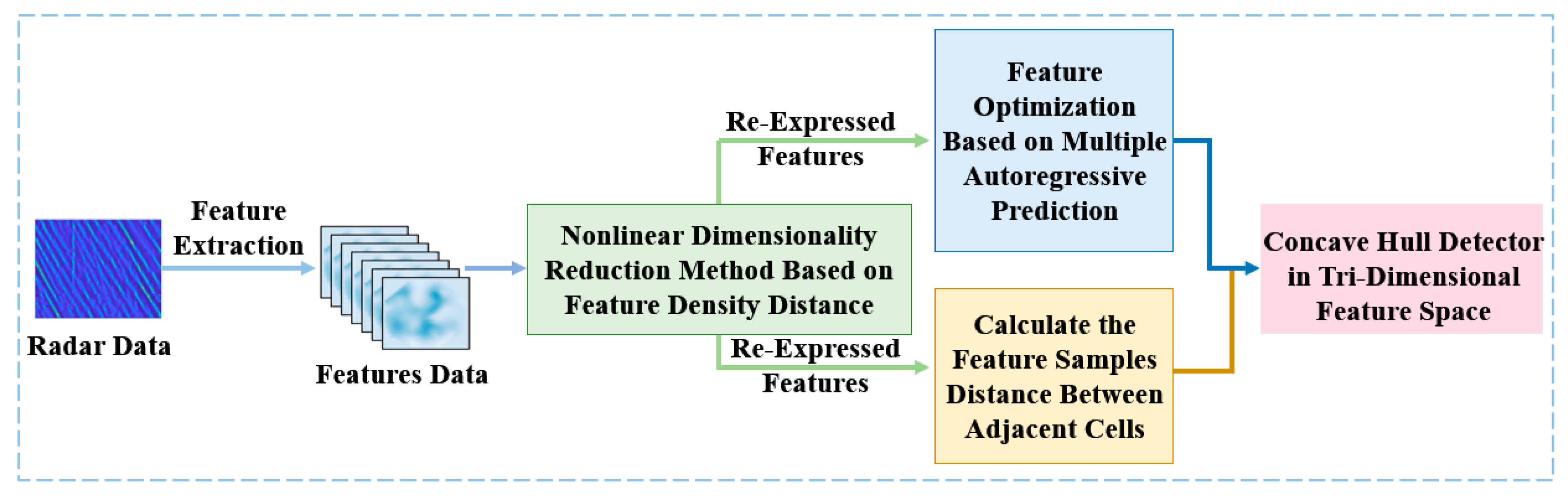
Extract feature samples using historical frame sea clutter data from the same scene and re-express the features using the method proposed in Section 3.2 to obtain sample sequences of three new features.

(2)

Calculate and statistically analyze the feature sample distances of adjacent clutter samples, then sort these distances from largest to smallest. Multiply the false alarm probability factor $\alpha$ by the sample quantity to select the corresponding index’s feature sample distance as the distance threshold $T_{\alpha }$. Here, the preset false alarm probability factor $\alpha$ for sample feature distance is 10⁻³.

(3)

Construct the concave hull decision region using historical clutter feature samples after removing false alarm control vertices [19].

(4)

Extract the features of the current CUT and its adjacent RC, then perform nonlinear re-expression to obtain the sample sequences of three new features.

(5)

Calculate the feature sample distance between adjacent cells and compare it with the threshold $T_{\alpha }$. If the distance is less than the threshold, classify the CUT as clutter; if it is greater than the threshold, proceed to step (6) for further judgment.

(6)

Compare the relative position of the RC sample and the concave hull decision region in the three-dimensional feature space. If the RC sample is within the concave hull, classify the CUT as a target; if the RC sample is outside the concave hull, classify the CUT as clutter. This step is executed only if the feature sample distance in step (5) exceeds the threshold.

This detector utilizes feature sample distance and the high accuracy of clutter sample detection to avoid the dispersion problem of target samples. When the RC sample is correctly judged as clutter, if the feature sample distance between the CUT and the RC at that time is larger than the threshold, the feature sample of the CUT is judged as a target; otherwise, it is judged as clutter. There is a possibility of false alarm here, i.e., although the RC sample is judged as clutter, its true class may be a more dispersed target sample. At this time, due to the large feature sample distance, the clutter of the CUT is judged as a target, resulting in a false alarm. However, as shown in Figure 14, the selection of the CUT and the RC is reciprocal. When the original RC is detected as a CUT, it will also be judged as a target, and the adjacent targets will be synthesized into a larger target spanning multiple range cells, thus offsetting the negative impact of such false alarms.

3.4. Feature Optimization Based on Multivariate Autoregressive Prediction

In Section 3.3, the detection decision for targets in the feature space is transformed into a detection decision for clutter. Although sea clutter samples exhibit less dispersion in the feature space compared with target samples, they are more susceptible to generating a small number of outliers due to real-world issues such as sea spikes, causing them to deviate from the clutter concave hull region and resulting in false alarms. This problem is particularly evident when extracting feature samples from short pulse time series, which can increase the feature variance. To address this problem, we propose a feature optimization method based on multivariate autoregressive prediction. This method uses the observed values of historical feature samples to predict the feature samples at the current time and then performs a weighted fusion of the predicted values and observed values to reduce the negative impact of outlier samples.

The predicted coordinates of the feature sample in the feature space at time t are given by the following equation:

$$\begin{array}{cc}{\widehat{g}}_t& ={(g_{t,1},g_{t,2},g_{t,3})}^{\mathrm{T}}=C+{\displaystyle \sum _{k=1}^p{A}_k{g}_{t-k}}\\ & =(c_1,c_2,c_3)+{\displaystyle \sum _{k=1}^p\left[\begin{array}{ccc}{a}_{k,11}& a_{k,12}& a_{k,13}\\ a_{k,21}& a_{k,22}& a_{k,23}\\ a_{k,31}& a_{k,32}& a_{k,33}\end{array}\right]{(g_{t-k,1},g_{t-k,2},g_{t-k,3})}^{\mathrm{T}}}\end{array}$$

(38)

where ${\widehat{g}}_t$ is the predicted coordinate of the feature sample in the feature space at time t, ${\widehat{g}}_{t,i}$ is the predicted value of feature $g_i$ at time t. $g_{t-k}$ is the observed coordinate of the feature sample in the feature space at time t−k, and $g_{t-k,i}$ is the observed value of the feature $g_i$ at time t−k. $A_k$ is the coefficient matrix at time k, $C$ is the constant matrix, and $p$ is the order of the prediction.

Before fitting the coefficient matrix with the autoregressive model, it is necessary to determine the prediction order $p$ of the fitting model. The appropriate order of the AR model can be determined by the Partial Autocorrelation Coefficient (PAC) of the feature sequence. The PAC of the feature sample $g_i$ is defined as (39).

$${\rho }_{g_{t,i},g_{t-k,i}|g_{t-1,i},\cdots ,g_{t-k+1,i}}={\displaystyle \frac{\mathrm{E}\left[\left(x_{t,i}-\stackrel{\wedge }{\mathrm{E}}(g_{t,i}|g_{t-1,i},\cdots ,g_{t-k+1,i})\right)\left(g_{t-k,i}-\stackrel{\wedge }{\mathrm{E}}(g_{t-k,i}|g_{t-1,i},\cdots ,g_{t-k+1,i})\right)\right]}{\mathrm{E}\left[\left.{\left(g_{t-k,i}-\stackrel{\wedge }{\mathrm{E}}(g_{t-k,i}|g_{t-1,i},\cdots ,g_{t-k+1,i})\right)}^2\right]\right.}}$$

(39)

where $\mathrm{E}(·)$ represents expectation. PAC is the ratio of the conditional autocovariance function to the conditional variance, essentially the conditional autocorrelation coefficient. By calculating the PAC value of the feature sequence, the lag order at which the PAC value first becomes insignificant is identified as the prediction order $p$. Here, PAC values below zero are defined as insignificant. Figure 15 shows the PAC curves for the three new features obtained through nonlinear dimensionality reduction in Section 3.2. It can be seen that their respective prediction orders $p$ are similar, so the maximum insignificant point is taken as the prediction order.

Next, the least squares estimation method is used to estimate the total coefficient matrix $B$. First, $N$ feature samples are arranged according to the prediction order $p$ to form the lag matrix $Z$. Then, the $N-p$ samples from time $p+1$ to time $N$ are arranged as the sample observation matrix $Y$, as shown in (40).

$$Z=\left[\begin{array}{cccc}{g}_p^{\mathrm{T}}& g_{p-1}^{\mathrm{T}}& \cdots & g_1^{\mathrm{T}}\\ g_{p+1}^{\mathrm{T}}& g_p^{\mathrm{T}}& \cdots & g_2^{\mathrm{T}}\\ ⋮& ⋮& \ddots & ⋮\\ g_{N-1}^{\mathrm{T}}& g_{N-2}^{\mathrm{T}}& \cdots & g_{N-p}^{\mathrm{T}}\end{array}\right], Y=\left[\begin{array}{c}{g}_{p+1}^{\mathrm{T}}\\ g_{p+2}^{\mathrm{T}}\\ ⋮\\ g_N^{\mathrm{T}}\end{array}\right]$$

(40)

Thus, the objective of the least squares method is to find the optimal total coefficient matrix $B$, which minimizes the sum of the squared errors between the predicted values and the observed values of the samples, as shown in the objective function equation (41).

$$\underset{B}{\arg \min }{‖Y-ZB‖}^2$$

(41)

By differentiating the objective function and setting it to zero, the analytical solution for the coefficient matrix $B$ can be obtained, as shown in (42).

$$B={(Z^{\mathrm{T}}Z)}^{-1}{Z}^{\mathrm{T}}Y$$

(42)

Since the total coefficient matrix $B$ includes both the constant term and the coefficient matrix $A$, it needs to be separated to obtain the constant matrix $C$, as shown in (43):

$$C={\displaystyle \frac{1}{N-p}}{\displaystyle \sum _{t=p+1}^N(g_t^{\mathrm{T}}-Z_{t-p}B)}$$

(43)

where $Z_{t-p}$ represents the $t-p$ th row of the lag matrix $Z$, corresponding to the previous $p$ observations needed for the feature sample at the prediction time t.

Finally, the total coefficient matrix $B$ is reshaped to a dimension of 3 × 3 × p, resulting in the coefficient matrix $A$ to represent the influence of each lag time, as shown in (44).

$$A=[A_1,A_2,\dots ,A_p]=\mathrm{reshape}(B,(3,3,p))$$

(44)

Now, the complete multivariate regression prediction parameters have been obtained. The prediction performance of the algorithm was tested using measured data, and the results are shown in Figure 16. It can be observed that the prediction value curves of each feature sample have a small error compared with the observed sequences, demonstrating good predictive performance.

Next, as shown in Figure 17, the predicted values of the feature sample coordinates are combined with the observed values using equal weights to obtain the fused coordinates of the feature samples in the three-dimensional feature space. These fused coordinates are then used in the decision-making process of the method proposed in Section 3.3, specifically in determining the relative spatial position with respect to the concave hull decision region. This process effectively smooths the observed values of the feature samples, reducing erroneous detections caused by outlier samples and lowering the variance of the features. The complete process of the proposed small maritime target detection method using nonlinear dimensionality reduction and feature sample distance is shown in Figure 18.

4. Performance Analysis and Discussion

This section uses eight sets of data under different sea state conditions, ranging from 2 to 5, from the SDRDSP dataset introduced in Section 2.1 to test and analyze the performance of the proposed method. Each dataset consists of complex time series with a length of 2¹⁷ from 950 or 1000 adjacent range cells (depending on the mode), corresponding to approximately 65 s. A feature sample is calculated for every 256-length time series using a sliding window with a size of 64. Each set of data yields over 2000 valid feature samples at each range cell. The number of feature samples used for verification accounts for half of the total sample size. Five comparison methods are also established, including three feature re-expression detection methods: the PCA-based target feature detection method [25], the LDA-based target feature detection method [26], and the feature compression-based target detection method [15]; and two target detection methods that directly construct three-dimensional feature spaces using different features: one using the three most separable features and the other using the RAA, RPH, and RVE features selected in the literature [8]. To control the conditions of the comparison experiments and eliminate the influence of feature types and quantities on the detector itself, the features and decision methods used in some detection methods are adjusted. For the PCA and LDA-based target feature detection methods, the features are expanded from the default six features to all eleven features introduced earlier. For the feature compression-based target detection method, the features are expanded from the originally defined seven features to the eleven features mentioned earlier. All detection methods use a concave hull detector, as described in [19,33], within the corresponding three-dimensional feature space.

To analyze the interaction relationships among multiple features during the classification process and compare the performance of the detection methods, the feature samples used for decision-making by each method are displayed in the three-dimensional feature space under sea state 5 and a false alarm probability of 10⁻³, and the decision regions of the concave hull classifier are plotted, as shown in Figure 19. In Figure 19a–e, the feature samples are extracted from the target at the CUT, with red samples being correctly classified as targets outside the concave hull and green samples being incorrectly classified as clutter inside the concave hull. Figure 19f shows the feature space of the proposed method, where the feature samples are extracted from the adjacent RC of the CUT where the target is located. Green samples are inside the concave hull, and the feature sample distance to the CUT is greater than the threshold, thus correctly identifying the adjacent target cell as a target; red samples are outside the concave hull, incorrectly identifying the adjacent target cells as clutter; blue samples are inside the concave hull, but the feature sample distance to the CUT is less than the threshold, thus incorrectly identifying the adjacent target cell as clutter.

Observing Figure 19a,b, it can be found that in the LDA and PCA feature re-expression target detection methods, the two classes of samples detected as targets and clutter only show significant distinction in the main feature 1 direction, meaning main feature 1 plays a supporting role in the classification problem, while the contributions of main features 2 and 3 are almost zero, and the problem of feature redundancy is not resolved through feature dimensionality reduction. The clutter concave hull decision region is large, resulting in a considerable proportion of target feature samples being incorrectly classified. The target samples show a significant dispersion trend in the direction opposite to the concave hull, indicating that in these two feature spaces, the feature sample distance still has good discrimination when adjacent cells contain different sample types. Constructing a feature space using the RAA, RPH, and RVE features, as shown in Figure 19c, reveals that although the concave hull decision region is small, many samples fall into it and are incorrectly detected, and the method is significantly affected by outlier samples marked by orange circles. Figure 19d shows the feature space constructed using the three features with the largest individual feature density distances, showing reduced incorrect detections but still being significantly affected by outlier samples and individual feature performance. In both feature spaces of Figure 19c,d, the dispersion trend of target samples is also present. Figure 19e shows the feature space constructed by three new features re-expressed by the feature compression algorithm. Compared with the previous four target detection algorithms, it has a smaller concave hull, and the three re-expressed features can complement each other, showing better classification capability. However, many incorrect detections still exist. Figure 19f shows the feature space of the proposed method, where the feature samples used are clutter feature samples from RC, not target feature samples from the CUT. It can be seen that since the convergence of clutter feature samples is much stronger than that of target samples, most samples can correctly fall within the concave hull. By associating the feature sample distance with the target samples of the CUT, most samples can be correctly classified. Compared with the comparison methods, the decision criteria in the feature space of the proposed detection method simultaneously utilize the dispersion of target samples and the convergence of clutter samples, resulting in higher accuracy.

Using measured data under different sea state conditions, the detection probability of the above six detection methods is calculated under a false alarm probability of 10⁻³, as shown in Figure 20. It can be seen that under low sea state conditions (sea states 2 and 3), all feature-based target detection methods achieve good detection results. However, as the data conditions change to sea state 3, the performance of all detection methods drops significantly, with the detection probability of the feature compression-based detection method, the three best feature density distance detection method, and the proposed method remaining above 85%. When the data conditions deteriorate to sea state 5, only the feature compression-based detection method and the proposed method maintain a detection probability above 75%, with the proposed method being about 4% higher than the former. At this time, the performance of the detection methods that construct feature spaces using fixed features is very poor. The PCA and LDA detection methods have low detection probabilities due to having only one effective feature.

Using measured data under sea state 5, the detection probability of the above six detection methods is calculated under different false alarm probability conditions, and the ROC curves are shown in Figure 21. It can be seen that under the same false alarm probability conditions, the proposed method has a higher detection probability than all comparison methods and has a smoother ROC curve, indicating that it is less affected by changes in false alarm probability and can provide more reliable detection performance in practical scenarios.

5. Conclusions

This study proposes a small maritime target detection method using nonlinear dimensionality reduction and feature sample distance. The nonlinear correlations of existing features in a multidimensional feature space were analyzed, and a feature density distance was defined. This distance was used as a loss function to design a lightweight nonlinear dimensionality reduction network on the basis of a self-attention mechanism, aiming to optimize the re-expression of the feature space. On the basis of this, a target detector using feature sample distance is proposed, which utilizes the RC samples in the feature space and the sample distance to the CUT to achieve comprehensive target detection. Additionally, a feature optimization method based on multivariate autoregressive prediction is proposed to reduce the negative impact of anomalous feature samples on detection performance. Testing with measured data shows that the proposed nonlinear dimensionality reduction method can generate re-expressed features with stronger joint classification capability and less information redundancy, which complement each other in the three-dimensional feature space. After feature optimization through multivariate autoregressive prediction, the proposed target detector based on feature sample distance demonstrated superior performance and stability under different sea states and false alarm probability conditions compared with the comparison methods.

References

1. Serafino, F.; Bianco, A. X-Band Radar Detection of Small Garbage Islands in Different Sea State Conditions. Remote Sens. 2024, 16, 2101. [Google Scholar] [CrossRef]
2. Shui, P.L.; Zhang, L.X. Small Target Detection in Sea Clutter by Weighted Biased Soft-Margin SVM Algorithm in Feature Spaces. IEEE Sens. J. 2024, 24, 10419–10433. [Google Scholar] [CrossRef]
3. Zhou, S.; Zhou, H. Detection Based on Semantics and a Detail Infusion Feature Pyramid Network and a Coordinate Adaptive Spatial Feature Fusion Mechanism Remote Sensing Small Object Detector. Remote Sens. 2024, 16, 2416. [Google Scholar] [CrossRef]
4. Xiong, G.; Wang, L. Radar Sea Clutter Reconstruction Based on Statistical Singularity Power Spectrum and Instantaneous Singularity Exponents Distribution. IEEE Trans. Geosci. Remote Sens. 2021, 59, 5687–5697. [Google Scholar] [CrossRef]
5. Xu, S.W.; Wang, Z. Optimum and near-optimum coherent false alarm rate detection of radar targets in compound-Gaussian clutter with generalized inverse Gaussian texture. IEEE Trans. Aerosp Electron. 2022, 58, 1692–1706. [Google Scholar] [CrossRef]
6. Shui, P.L.; Liu, M. Sub-band adaptive GLRT-LTD for weak moving targets in sea clutter. IEEE Trans. Aerosp. Electron. 2016, 52, 423–437. [Google Scholar] [CrossRef]
7. Shi, S.N.; Shui, P.L. Detection of low-velocity and floating small targets in sea clutter via income-reference particle filters. Signal Process. 2018, 148, 78–90. [Google Scholar] [CrossRef]
8. Shui, P.L.; Li, D.C. Tri-feature-based detection of floating small targets in sea clutter. IEEE Trans. Aerosp Electron. 2014, 50, 1416–1430. [Google Scholar] [CrossRef]
9. Shi, S.N.; Shui, P.L. Sea-surface floating small target detection by one-class classifer in time-frequency feature space. IEEE Trans. Geosci. Remote Sens. 2018, 56, 6395–6411. [Google Scholar] [CrossRef]
10. Xie, J.; Xu, X. Phase-feature-based detection of small targets in sea clutter. IEEE Geosci. Remote Sens. Lett. 2022, 19, 1–5. [Google Scholar] [CrossRef]
11. Guo, Z.X.; Shui, P.L.; Bai, X.H. Small target detection in sea clutter using all-dimensional Hurst exponents of complex time sequence. Digit. Signal Process 2020, 101, 102707. [Google Scholar] [CrossRef]
12. Li, D.C.; Shui, P.L. Floating small target detection in sea clutter via normalised Doppler power spectrum. IET Radar Sonar Navig. 2016, 10, 699–706. [Google Scholar] [CrossRef]
13. Qu, Q.; Wang, Y.L.; Liu, W.; Li, B. A false alarm controllable detection method based on CNN for sea-surface small targets. IEEE Geosci. Remote Sens. Lett. 2022, 19, 1–5. [Google Scholar] [CrossRef]
14. Shi, Y.L.; Guo, Y.X. Sea-surface small floating recurrence plots FAC classification based on CNN. IEEE Trans. Geosci. Remote Sens. 2022, 60, 1–13. [Google Scholar] [CrossRef]
15. Shui, P.L.; Guo, Z.X. Feature-compression-based detection of sea-surface small targets. IEEE Access. 2020, 8, 8371–8385. [Google Scholar] [CrossRef]
16. Guo, Z.X.; Shui, P.L. Anomaly-based sea-surface small target detection using K-nearest-neighbor classification. IEEE Trans. Aerosp. Electron. Syst. 2020, 56, 4947–4964. [Google Scholar] [CrossRef]
17. Li, Y.; Xie, P. SVM-based sea-surface small target detection: A false-alarm-rate-controllable approach. IEEE Geosci. Remote Sens. Lett. 2019, 16, 1225–1229. [Google Scholar] [CrossRef]
18. Chen, S.; Ouyang, X.; Luo, F. Ensemble One-Class Support Vector Machine for Sea Surface Target Detection Based on K-Means Clustering. Remote Sens. 2024, 16, 2401. [Google Scholar] [CrossRef]
19. Wu, X.; Ding, H.; Liu, N.B. A method for detecting small targets in sea surface based on singular spectrum analysis. IEEE Trans. Geosci. Remote Sens. 2022, 60, 1–17. [Google Scholar] [CrossRef]
20. Shi, Y.L.; Hu, Y.F. mRMR-Tri-ConcaveHull detector for the floating small targets in sea clutter. IEEE J. Sel. Top. Appl. Earth Obs. Remote Sens. 2023, 16, 6799–6811. [Google Scholar] [CrossRef]
21. Zhou, H.K.; Jiang, T. Decision tree based sea-surface wake target detection with false alarm rate controllable. IEEE Signal Process Letter. 2019, 26, 793–797. [Google Scholar] [CrossRef]
22. Su, N.; Chen, X. Radar Maritime Target Detection via Spatial–Temporal Feature Attention Graph Convolutional Network. IEEE Trans. Geosci. Remote Sens. 2024, 62, 1–15. [Google Scholar] [CrossRef]
23. Wu, J.; Ni, R.; Chen, Z.; Huang, F.; Chen, L. FEFN: Feature Enhancement Feedforward Network for Lightweight Object Detection in Remote Sensing Images. Remote Sens. 2024, 16, 2398. [Google Scholar] [CrossRef]
24. Guo, Z.X.; Bai, X.H. Fast Dual Trifeature-Based Detection of Small Targets in Sea Clutter by Using Median Normalized Doppler Amplitude Spectra. IEEE J. Sel. Top. Appl. Earth Obs. Remote Sens. 2023, 16, 4050–4063. [Google Scholar] [CrossRef]
25. Gu, T. Detection of small floating targets on the sea surface based on multi-features and principal component analysis. IEEE Geosci. Remote Sens. Lett. 2020, 17, 809–813. [Google Scholar] [CrossRef]
26. Ali, H.; Bahari, N.I.; Elshaikh, M. Shape Recognition of GPR Images using Hough Transform and PCA plus LDA. In Proceedings of the 2022 2nd International Conference on Electronic and Electrical Engineering and Intelligent System (ICE3IS), Yogyakarta, Indonesia, 4–5 November 2022; pp. 387–391. [Google Scholar] [CrossRef]
27. Liu, N.B.; Dong, Y.L.; Wang, G.Q. Annual progress of the sea-detecting X-band radar and data acquisition program. J. Radars 2021, 10, 173–182. [Google Scholar] [CrossRef]
28. Guan, J.; Liu, N.B.; Wang, G.Q. Sea-detecting Radar Experiment and Target Feature Data Acquisition for Dual Polarization Multistate Scattering Dataset of Marine Targets. J. Radars 2023, 12, 456–469. [Google Scholar] [CrossRef]
29. Wang, J.H.; Wang, Z.H.; He, Z.S. GLRT-based polarimetric detection in compound-Gaussian sea clutter with inverse-Gaussian texture. IEEE Geosci. Remote Sens. Lett. 2022, 19, 1–15. [Google Scholar] [CrossRef]
30. Yu, W.; Yang, G.; Zhao, H. A new method for ship length estimation based on Doppler spectrum analysis. Radar Sci. Technol. 2015, 12, 522–526. [Google Scholar] [CrossRef]
31. Wu, X.J.; Ding, H. A Method for Detecting Small Targets in Sea Surface Based on Ridges-Radon Transform. J. Signal Process. 2021, 37, 1599–1611. [Google Scholar] [CrossRef]
32. Huang, Y.; Zhang, Z.; Li, X. Layered-Vine Copula-Based Wind Speed Prediction Using Spatial Correlation and Meteorological Influence. IEEE Trans. Instrum. Meas. 2023, 72, 1–12. [Google Scholar] [CrossRef]
33. Guan, J.; Wu, X.J.; Ding, H. Detection of Small Targets on Sea Surface Based on 3-D Concave Hull Learning Algorithm. J. Electron. Inf. Technol. 2023, 45, 1602–1610. [Google Scholar] [CrossRef]
Figure 1. Channel buoy: (a) Light buoy 1 (2.97 nmiles); (b) Light buoy 2 (3.19 nmiles).
Remotesensing 16 02901 g001
Figure 2. Sea state conditions of SDRDSP.
Remotesensing 16 02901 g002
Figure 3. Amplitude distribution on target and sea clutter cells.
Remotesensing 16 02901 g003
Figure 4. The Bhattacharyya distance of each feature.
Remotesensing 16 02901 g004
Figure 5. The correlation between RAA and RVE under sea state 4: (a) Clutter feature samples; (b) Target feature samples.
Remotesensing 16 02901 g005
Figure 6. The correlation between RAA and RVE under sea state 5: (a) Clutter feature samples; (b) Target feature samples.
Remotesensing 16 02901 g006
Figure 7. Polynomial nonlinear fitting in three-dimensional feature space: (a) RVE, RDPH, and SOFE; (b) RAA, TEM, and RPH.
Remotesensing 16 02901 g007
Figure 8. Trend of feature density distance component variation.
Remotesensing 16 02901 g008
Figure 9. Comparisons of different λ density : (a) Smaller λ density ; (b) Larger λ density .
Remotesensing 16 02901 g009
Figure 10. The effect of density component η on false alarm control vertex: (a) Large λ density with no false alarms control; (b) Large λ density with false alarms control; (c) Small λ density with no false alarms control; (d) Small λ density with false alarms control.
Remotesensing 16 02901 g010
Figure 11. Nonlinear dimensionality reduction method based on feature density distance.
Remotesensing 16 02901 g011
Figure 12. The feature sample distance in feature spaces of different dimensions: (a) Clutter feature sample distance; (b) Target feature sample distance.
Remotesensing 16 02901 g012
Figure 13. Probability density curves of feature sample distances between adjacent cells in different situations: (a) Under sea state 2; (b) Under sea state 5.
Remotesensing 16 02901 g013
Figure 14. Merge false alarm cells into targets across range cells.
Remotesensing 16 02901 g014
Figure 15. The PAC curves: (a) The feature samples re-expressed at clutter cell; (b) The feature samples re-expressed at target cell.
Remotesensing 16 02901 g015
Figure 16. Prediction feature samples and prediction error: (a) The feature samples re-expressed at clutter cell; (b) The feature samples re-expressed at target cell.
Remotesensing 16 02901 g016
Figure 17. The generation of fused feature samples.
Remotesensing 16 02901 g017
Figure 18. Marine small target detection method based on nonlinear dimensionality reduction and feature sample distance.
Remotesensing 16 02901 g018
Figure 19. Three-dimensional Feature Space Position Relationship Diagram: (a) LDA; (b) PCA; (c) Target detection method using the RAA, RPH, and RVE; (d) Target detection method using three features with the largest individual feature density distances; (e) The feature compression-based target detection method; (f) The proposed method.
Remotesensing 16 02901 g019
Figure 20. Comparison of detectors under different sea states.
Remotesensing 16 02901 g020
Figure 21. Comparison of methods under different false alarm probabilities.
Remotesensing 16 02901 g021