1. Introduction
Due to the rapid development of imaging technology, the processing and analysis of remote-sensing images have become increasingly important. Consequently, the automatic extraction of fundamental information from remote-sensing images has become a key research direction in the field of remote-sensing image processing [
1]. Remote-sensing land-cover segmentation is critical for analyzing remote-sensing images, playing a key role in processing and utilizing remote-sensing data. By employing image semantic-segmentation algorithms, it assigns categories to each pixel of remote-sensing images, identifying various landforms and extracting essential information [
2]. In military contexts, it provides crucial intelligence for tactical and strategic operations. Environmentally [
3], it aids in quickly and accurately detecting ecological changes, while in urban development, it supports city planning and the enhancement of infrastructure. Geospatial clarity is also improved in geoscience, establishing an important base for earth studies. The wide-ranging utility of this technology underscores the need for precision in remote-sensing segmentation methods. Remote-sensing images contain abundant surface feature information, yet accurately segmenting real-world regions remains a long-standing challenge [
4,
5,
6]. Traditional segmentation methods [
7,
8,
9], such as threshold-based segmentation, edge detection, and pixel clustering, have limited robustness and struggle to extract deep semantic information from images.
The swift advancement of deep learning techniques, particularly convolutional neural networks (CNNs), has made them an essential tool in the field of computer vision due to their powerful capability for feature extraction. Several scholars have successfully applied CNNs to tasks related to remote-sensing image segmentation [
10]. Zheng [
11] developed FarSeg, a foreground-aware relational network designed to address significant intraclass variance in background classes and the imbalance between foreground and background in remote-sensing images. In 2021, Li [
12] introduced Fctl, a geospatial segmentation approach based on location-aware contexts, which systematically crops and independently segments images, later merging these to form a cohesive output. Zheng et al. proposed SETR [
13] to improve the model’s ability to understand complex contextual relationships in images by exploiting the contextual information capture ability of transformers. Additionally, Ma [
14] introduced FactSeg, utilizing the foreground activation object representation to enhance detection and differentiation of smaller objects.
Recent studies on object detection highlight the critical role of foreground saliency in remote-sensing image analysis. Various researchers, inspired by these findings, have been adapting transformer architectures for remote object detection. Segformer [
15] designed a hierarchically structured transformer-based encoder and a decoder consisting of several layers of lightweight multi-layer perceptrons. Xu introduced the Efficient Transformer [
16], which exhibits improved computational efficiency and uses explicit and implicit edge-enhancement techniques for precise segmentation. Wang [
17] presented a design using the Swin Transformer for context extraction from images and introduced a densely connected feature aggregation setup for resolution restoration and intricate segmentation. Xu proposed the RSSFormer [
18], a remote-sensing object segmentation framework with an adaptive transformer conjunction module, attention layer, and a foreground prominence-based loss function, designed to reduce background noise and enhance foreground differentiation. Sanghyun Woo [
19] proposed CBAM in 2018, with the main goal of improving the perception ability of the model by introducing channel attention and spatial attention into CNNs.
Land-cover segmentation poses distinct challenges compared to standard semantic segmentation, which include significant variance in object sizes even within the same class, like large forests versus isolated trees; complex background components in remote-sensing images, making it difficult to classify certain elements into defined segments; and prevalence of background over foreground, which could bias the model to favor background segmentation during training, potentially affecting its optimization path.
In this paper, the prominent contributions are as follows:
We propose a module called multi-dilation rate convolutional fusion module. A corresponding module integrates outputs from convolutions with different dilation rates, addressing dilated convolution’s information loss and improving scale-variant target segmentation.
We introduce a hybrid attention module called large-kernel selection hybrid attention module, grounded on large-kernel convolutions. In the spatial attention submodule, we embed a convolutional kernel selection strategy to accommodate varying segmentation scales. For channel attention, we consider a large-kernel convolution-based attention to enhance the model’s receptive scope, thereby improving its foreground–background distinction and suppressing unrelated background noise. Combining this with multi-dilation rate convolutional fusion module results in the multi-dilation and large-kernel convolution-based decoder.
The rest of this paper is organized as follows.
Section 2 presents a diagram of the decoder system we designed and introduces the workflow of the system. This is then followed by an introduction to the principles and network structure of the fusion decoder based on multi-dilation rate convolution along with the hybrid attention module based on the large-kernel convolution selection.
Section 3 describes the datasets and implementation details used.
Section 4 provides discussions.
Section 5 draws conclusions.
2. Methods
2.1. Multi-Dilation and Large-Kernel Convolution-Based Decoder
The structure of our multi-dilation and large-kernel convolution-based decoder is shown in
Figure 1.
We propose an improved decoder workflow aimed at enhancing the performance of image segmentation. In this process, we draw on the widely recognized encoder-decoder architecture in the field of image segmentation, with particular reference to the Segformer and HRNet models. While retaining the original encoder, we have optimized the decoder. Specifically, we have replaced the All-MLP decoder of Segformer and the upsampling part of HRNet with the multi-dilation rate convolutional fusion module and large-kernel-selection hybrid attention module.
The input image is first processed by the encoder to extract feature maps at various resolutions. These feature maps then enter the decoder. Here, the multi-scale feature maps are first sent to the large-kernel-selection hybrid attention module. This module uses spatial attention and channel attention modules based on a large-kernel convolution selection mechanism to perform hybrid processing on the feature maps. The processed feature maps are then sent to the multi-dilation rate convolutional fusion module. Within the module, the feature maps undergo three convolution-batchnorm-activation modules processing steps, followed by upsampling, feature-map fusion, and convolution operations, ultimately generating the decoded output. This decoder not only improves the processing efficiency of the feature maps but also enhances the accuracy of image segmentation.
2.2. Multi-Dilation Rate Convolutional Fusion Module
To counter the challenges in land-cover segmentation, we delineate the construction of a decoder tailored for the segmentation of objects within remote-sensing imagery, named the Multi-Dilation Rate Convolutional Fusion Decoder (MDCFD). Drawing inspiration from the decoders of Segformer and SETR, alongside extant encoder–decoder frameworks, the conceived MDCFD embodies a comparatively simplistic structure of multiple multi-layer perceptrons. In a bid to augment the saliency of foreground features within the decoder’s feature maps, this exposition integrates the Rssformer paradigm into the architecture of MDCFD through the adoption of dilated convolutions, with the intent to accentuate foreground details during the decoding phase. Dilated convolutions leverage enlarged kernels to span a wider sampling domain, thereby bridging distant pixels and infusing additional contextual data.
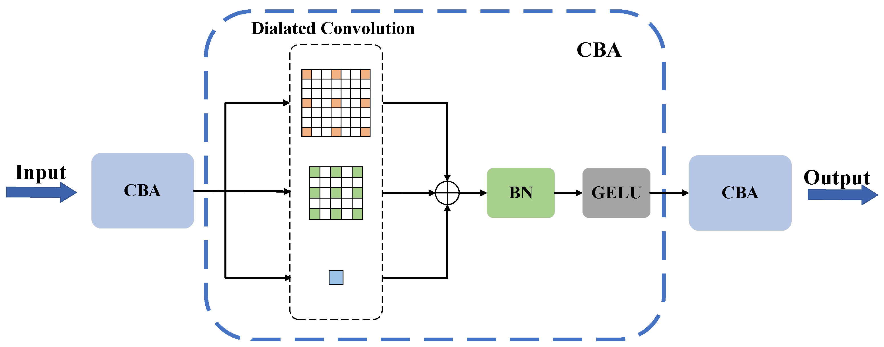
To adeptly tackle the issue of pronounced size variability among analogously classified objects within remote-sensing imagery, we introduce the Multi-Dilation Rate Convolutional Fusion Module (MDCFM) in MDCFD. Said module employs dilated convolutions with minimal dilation rates for the delineation of fine-detail features inherent to smaller objects, while those with escalated dilation rates apprehend an extended feature spectrum. Subsequently, the MDCFM amalgamates the feature maps, processed via convolutional layers possessing divergent receptive fields across multiple convolutional trajectories, through an element-wise addition methodology. The structure of the MDCFM is as depicted in
Figure 2.
Input feature maps are processed through sequential processing through three CBAs (Convolution–BatchNorm–Activation), each a composite of convolutional, batch normalization, and activation layers in a serial configuration. We incorporate the Gaussian Error Linear Unit (GELU) as the activation function within the CBA modules, with the computational progression of these modules delineated as
where
represents the input feature maps and
is the output of the CBA, with
indicating batch normalization. The CBA in the sequence includes two dilated convolutions with dilation rates of 2 and 3, plus a convolution (dilation rate of 1), facilitating feature integration across various receptive fields via element-wise addition. The module’s computational progression is outlined as
where
represents the output feature map that results from the fusion of multiple dilated convolutions, and
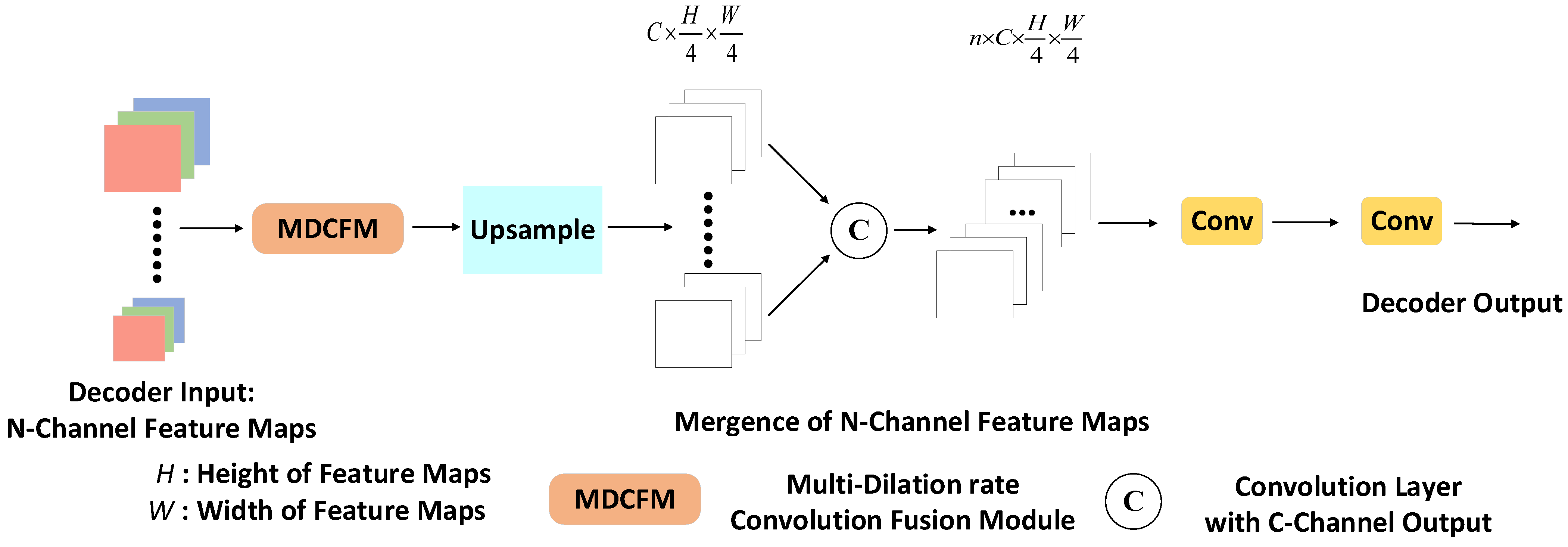
refers to the dilated convolution operation with a kernel size of 3 and a dilation rate of 2. This approach captures multi-scale context information through different dilation rates, effectively generating enriched feature representation and enhancing the module’s adaptability to complex, varied spatial structures in remote-sensing images through an element-wise addition operation. The construction of MDCFD is shown in
Figure 3.
After processing by the MDCFM, the n-channel feature maps are subjected to bilinear upsampling within the upsampling module, which helps to ensure consistency in spatial features. The upsampling increases the map resolution to a quarter of its original width and height, avoiding a direct return to the original resolution. This strategic choice theoretically reduces computational and memory demands while maintaining the spatial detail needed for accurate semantic segmentation. Finally, the feature maps are merged through channel concatenation, followed by a convolutional layer that outputs -channels, to generate the final output of the decoder
2.3. Large-Kernel-Selection Hybrid Attention Module
Inspired by the CBAM, we devised a large-kernel-selection hybrid attention module (LKSHAM) that adopts similar dual-submodule framework, as detailed in
Figure 4. Within this framework, the initial output
is directed through a channel attention module to generate an attention mask
(Equation (3)). This mask is then applied element-wise to
, yielding a channel-enhanced feature map
(Equation (4)). Subsequently, the enhanced feature map
is refined by the spatial attention module, generating a spatial attention mask
which serves to sharpen the spatial focus (Equation (5)). The final output,
, is obtained by combining the mask
with the feature map
, signifying an increased concentration of attention, as expressed by Equation (6).
2.3.1. Large-Kernel-Selection Spatial Attention Module
Taking inspiration from SKNet and LSKNet [
20], this manuscript introduces a novel spatial attention module, denoted as the Large-Kernel-Selection Spatial Attention Module (LKSSAM), which integrates large-kernel convolutions with a convolutional kernel selection mechanism.
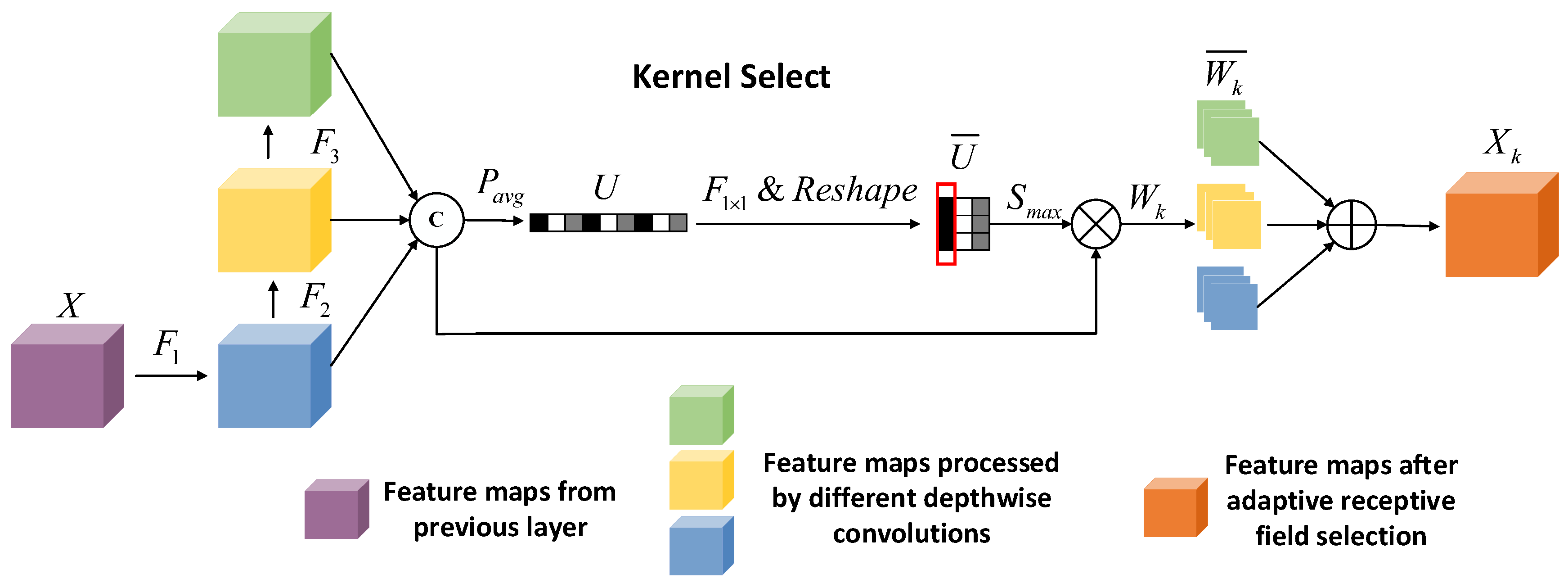
Figure 5 illustrates the procedural mechanics of the convolutional kernel selection mechanism. The output feature map
from the previous network layer, characterized by a batch size
and a channel count
, is subjected to a triad of depthwise convolutions:
,
, and
, derived from an expansive kernel convolution with a receptive field of 17 × 17. The dimensions of the kernel for
are stipulated as 3 × 3 with a corresponding dilation rate of 1, for
a kernel size of 5 × 5 with a dilation rate of 2, and for
, a kernel size of 3 × 3 with a dilation rate of 3 is established.
traverses the aforementioned paths
,
, and
to procure respective outputs
,
, and
, as expounded in the subsequent equation.
After individual operations,
,
, and
are combined through channel-wise (at dimension dim = 1) to form
as shown in Equation (8).
then undergoes global average pooling
, resulting in
.
, after a 1 × 1 convolution maintaining channels at
and then expanding and reshaping, becomes the five-dimensional matrix
, as described in Equations (9) and (10). Applying Softmax
to
’s next-to-last dimension yields the kernel selection weights matrix
, per Equation (11).
contains
sets of convolutional kernel selection weights, where the three elements within the kernel selection weights correspond to the selection coefficients for feature maps with different receptive fields after operations
,
, and
. After reshaping
to the shape of
, multiplicative interaction with
yields
, as depicted in Equation (12). Subsequently,
is divided along the penultimate dimension into three matrices, each with the shape of
. By performing an element-wise addition operation on these three matrices, the feature map
, post adaptive receptive field selection, is obtained. This process is detailed in Equation (13), where
denotes the matrix partitioning.
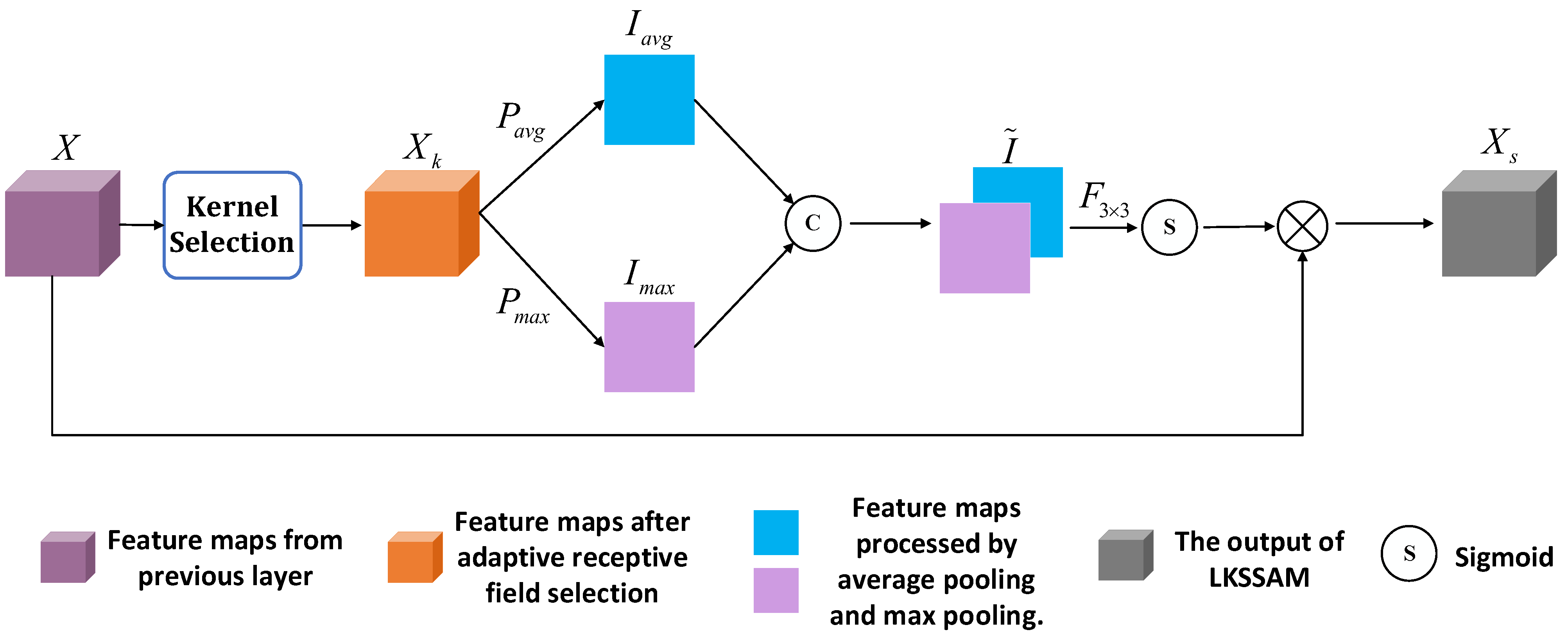
Figure 6 shows the complete schematic of the LKSSAM as presented in this article. The feature map
, after the kernel selection module, is subjected to both average and maximal pooling operations,
,
, yielding outputs
and
, as shown in Equation (14). Concatenating
and
along the channel axis results in matrix
, characterized by Equation (15). Subsequent to the processing of
through a convolutional maneuver
with an output channel quantum fixed at 1 and a 3 × 3 kernel dimension, succeeded by a Sigmoid activation, a spatial attention mask matrix
with elemental values confined within the interval (0, 1) comes to fruition, as delineated in Equation (16). The element-wise product of
with the antecedent input
begets the LKSSAM-augmented construct
, as depicted in Equation (17).
2.3.2. Large Kernel Channel Attention Module
We introduce a Large-Kernel Channel Attention Module (LKCAM), and by integrating with the LKSSAM, a Hybrid Attention Module (LKSHAM) is formed, capable of fully utilizing information from both spatial and channel dimensions.
The architecture of the LKCAM, as presented in this paper, is shown in
Figure 7. The output feature map
, with a batch size
and
channels from the previous layer of the neural network, first undergoes a 1 × 1 convolution
, reducing the channel number to
. To control the model’s parameterization scale, a channel reduction factor
is applied, reducing the channel count of the input feature map to a fraction of
, as shown in Equation (18)
Following the
, the output
is processed through two subsequent depthwise convolutions,
and
, as described in Equation (19). In this research,
is set with a dilation rate of 1, and
uses a 7 × 7 kernel with a dilation rate of 4. The sequence of
and
is equivalent to a single large-kernel convolution with a receptive field of 29 × 29. The feature map
, refined by this large-kernel convolution, is then passed through a 1 × 1 convolution that outputs
channels. This process restores the channel count of the final feature
to
, as shown in Equation (20).
is processed by a global max pooling layer and a global average pooling layer, resulting in matrices
and
, as presented in Equation (21). The result of adding
and
element-wise then enters a Sigmoid activation layer. The output from this layer forms the channel attention mask
, detailed in Equation (22). The values within
range from 0 to 1, indicating the weights assigned to the
channels by the channel attention module. Multiplying the output from the previous neural network layer element-wise with
yields the LKCAM-enhanced output
, as shown in Equation (23). This design allows the model to identify significant channels, emphasizing features that are crucial for the task while downplaying irrelevant channel information
After combining MDCFM and LHSHAM, and adding the necessary decoding output module, we obtain the decoder. The construction of the decoder is shown in
Figure 8.
3. Implementation and Results
3.1. Datasets and Data Pre-Processing
To evaluate the effectiveness of the described decoder, empirical tests were conducted using the ISPRS Potsdam and ISPRS Vaihingen datasets to assess its impact on segmentation accuracy. The results were then analyzed in detail. The datasets will be freely available at
www.isprs.org/education/benchmarks/UrbanSemLab/Default.aspx, accessed on 2 February 2024.
(1) The Potsdam dataset, recognized for advancing object segmentation and scene analysis, includes various image formats such as RGB, IRRG, and DSM. Our study selectively employed the RGB format for evaluation. Categorically, it covers six types of land cover: impervious surface, buildings, low vegetation, trees, cars, and miscellaneous areas (commonly termed as ‘clutter’).
(2) The Vaihingen dataset is key for advancing remote-sensing object segmentation research and applications. It mainly includes 33 ‘TOP’ high-resolution aerial images, with an average size of 2494 ∗ 2064 pixels. The Vaihingen dataset additionally provides detailed elevation data through Digital Surface Models (DSM) and Normalized Digital Surface Models (NDSM), with precise ground sampling accuracy up to 9 cm. Its object categories align with those in the Potsdam dataset. We exclusively utilized the ‘TOP’ images, without DSM and NDSM data.
(3) The high-resolution images from the Potsdam and Vaihingen datasets necessitate preprocessing through cropping to reduce memory load; hence, images were resized to 512 ∗ 512. We analyzed six land-cover categories from Potsdam and five corresponding categories from Vaihingen, excluding clutter, to evaluate the segmentation capability of our model.
3.2. Implementation Details
3.2.1. Hardware Environment
The methodology of this investigation involved the following hardware setup: an Intel Core i9-9900K CPU with a base frequency of 3.6 GHz, featuring 16 threads; an NVIDIA GeForce GTX 2080Ti GPU; and a computational platform for conducting experiments, equipped with 64 GB of memory and 4 TB of storage.
3.2.2. Software Environment
This article describes computational experiments that utilized Ubuntu 20.04 as the operating system and CUDA 11.3 for the parallel computing framework. To facilitate managing virtual environments necessary for model training and inference, this research utilized the Anaconda system. Detailed configurations are provided in the
Table 1.
3.2.3. Hyperparameter Settings
During the training regimen, the Adam optimizer was selected, featuring the beta coefficients of the Adam algorithm designated as 0.9 for and 0.999 for . The instructional rate for model training was established at 6 × 10⁻⁵, while the regularization term for weight decay was anchored at 0.01. The learning rate experienced adaptive alterations in line with the Poly learning rate policy, where the Poly power was defined as 1. We stopped after 160,000 epochs.
3.2.4. Common Evaluation Metrics for Land-Cover Segmentation
The commonly used evaluation metrics for land-cover segmentation algorithms include mean F1 score(mF1) and mean Intersection over Union (mIoU).
(1) The F1 score is the harmonic mean of precision and recall, which comprehensively considers the performance of these two metrics. Precision refers to the proportion of instances that are truly positive among those that the model predicts as positive samples. It measures the accuracy of the model’s predictions for positive samples. The formula for calculating precision can be referred to as Equation (24).
Here,
represents true positives: the number of instances correctly predicted as positive samples by the model;
represents false positives: the number of instances incorrectly identified as positive samples by the model. Recall refers to the proportion of all actual positive samples that are predicted as positive samples by the model. It measures the model’s ability to identify positive samples, that is, how many true positive samples are found. The formula for calculating recall can be seen in Equation (25).
Here,
represents false negatives: the number of instances incorrectly identified as negative samples by the model. For a single category, the formula for calculating the F1 score can be referred to as Equation (26).
The mF1 is the average of all category F1 scores, used to evaluate the model’s overall performance across all categories. Its calculation formula can be referred to as Equation (27).
Here, represents the total number of target categories, and represents the F1 score of the -th category.
(2) IoU refers to the ratio of the area of the intersection between the predicted region by the segmentation algorithm and the actual region to the area of their union. The calculation process can be seen in Equation (28).
Here,
represents the region predicted by the segmentation algorithm, and
represents the actual region. mIoU is the average value of the Intersection over Union for all categories. The specific calculation formula is shown in Equation (29).
3.3. Ablation Study
To establish the MDCFD decoder and LKSHAM’s accuracy, universality, and effectiveness, we merged them with top-performing models for comparative evaluation against original models. In our ablation studies, we first paired the MDCFD and LKSHAM with the Segformer’s MiT encoder, choosing the parameter-rich MiT-B5 encoder. Secondly, we combined them with HRNetV2 [
21], using the robust HRNetV2-W48 model. The outcomes are presented in
Table 2.
To assess the detection performance of the two modules suggested in this article, we compared the improved Segformer (named Seg&Ours) and HRNetV2 (named HRNetV2&Ours) models based on our proposal with conventional land-cover segmentation algorithms. The results are illustrated in
Table 3.
The results confirmed the significant enhancement in the performance of remote-sensing land-cover segmentation when the decoder we proposed was used in combination with two different encoder structures. The experimental results indicate that our decoder achieved notable improvements in the mIoU and mF1 accuracy metrics. Specifically, on the Potsdam dataset, our decoder increased the mIoU by 1.5% to reach 79.6%, and the mF1 by 1.2% to reach 87.6%, compared to the Segformer model. The segmentation accuracy for all categories improved compared to the baseline model, especially in the “car” category, where the accuracy increased by 1.8% after being combined with the HRNetV2 encoder. In experiments on the Vaihingen dataset, the mIoU improvement was up to 1.7%, reaching 82.1%, and the mF1 increased by up to 1.2 percentage points, reaching 90.1%. Particularly in the “car” category, after being combined with the HRNetV2 encoder, its accuracy increased by 2.4 percentage points compared to the baseline model. These results fully demonstrate that the decoder designed by us has a significant improvement in segmentation accuracy compared to traditional decoders.
3.4. Visual Results
3.4.1. Feature Map Analysis
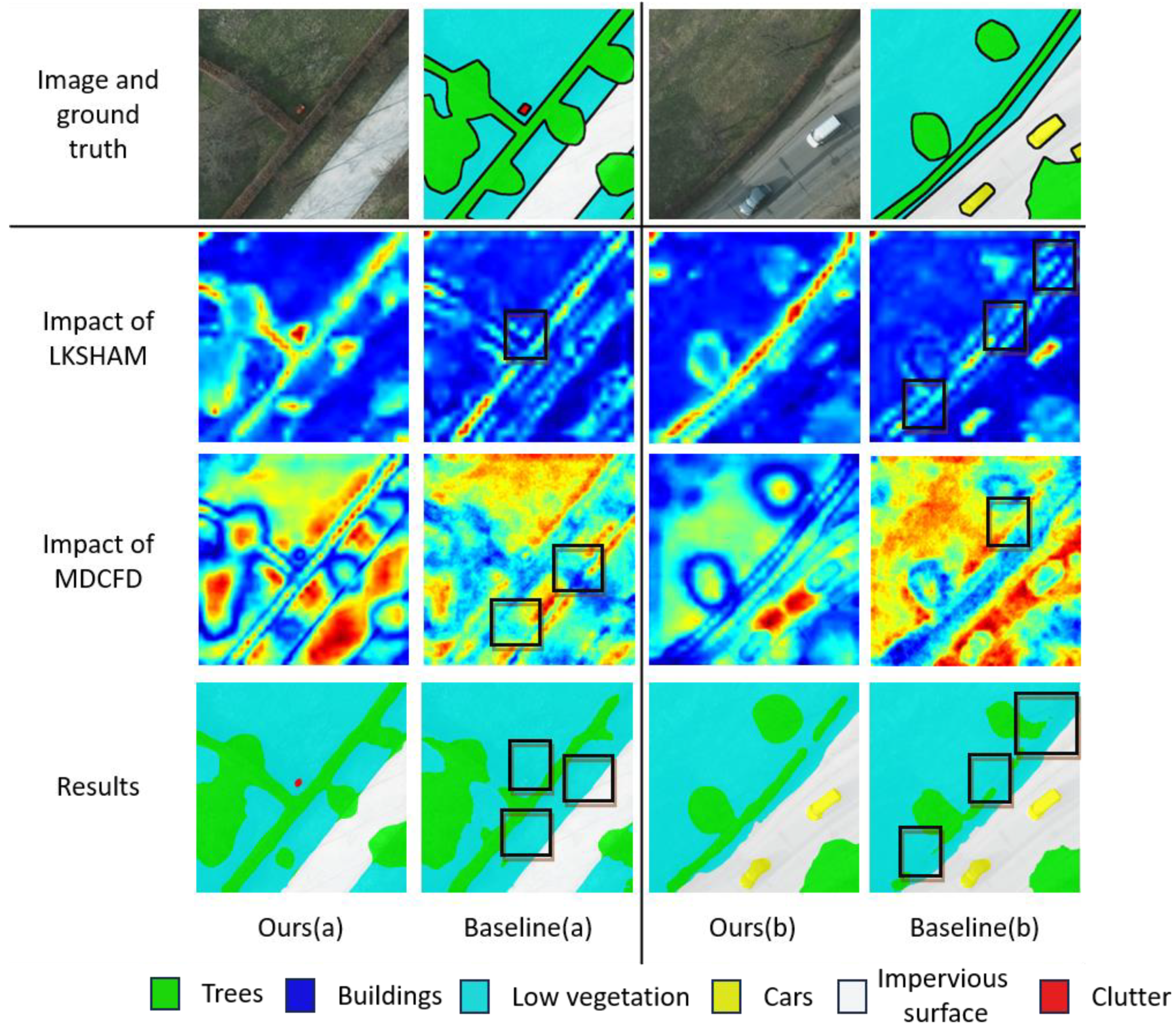
In
Figure 9a, the impact of the LKSHAM on feature maps is evident. The LKSHAM module enhances the extraction of features for small-scale targets (as indicated by the black box) by selecting an appropriate receptive field. This approach circumvents the issue observed in the baseline model, where such targets were not identifiable. Furthermore, the MDCFD integrates outputs from convolutions with varying dilation rates, synergizing with LKSHAM to enhance the segmentation capabilities across different scales of targets. In
Figure 9b, the influence of LKSHAM on feature maps is further elucidated. By incorporating large-kernel convolutions, the LKSHAM module bolsters the extraction of contextual information. Concurrently, the MDCFD leverages dilated convolutions to expand the receptive field, thereby enhancing the differentiation between the foreground and background. This strategy effectively addresses the shortcomings present in the baseline model, as illustrated by the black box.
3.4.2. Segmentation Results
Figure 10 graphically shows the improved segmentation accuracy of the system due to the MDCFD, using a set of image comparisons. As illustrated in
Figure 10c,d, the baseline algorithm performs poorly in segmenting the low vegetation marked by the red box in the images, while the algorithm improved with MDCFD can effectively recognize this low vegetation. Furthermore, in
Figure 10g,h, the system enhanced by MDCFD demonstrates superior performance in identifying cluttered scenes (as shown in the yellow boxes) compared to the baseline algorithm. These results confirm that MDCFD has better segmentation effects than the baseline algorithm in specific scenarios.
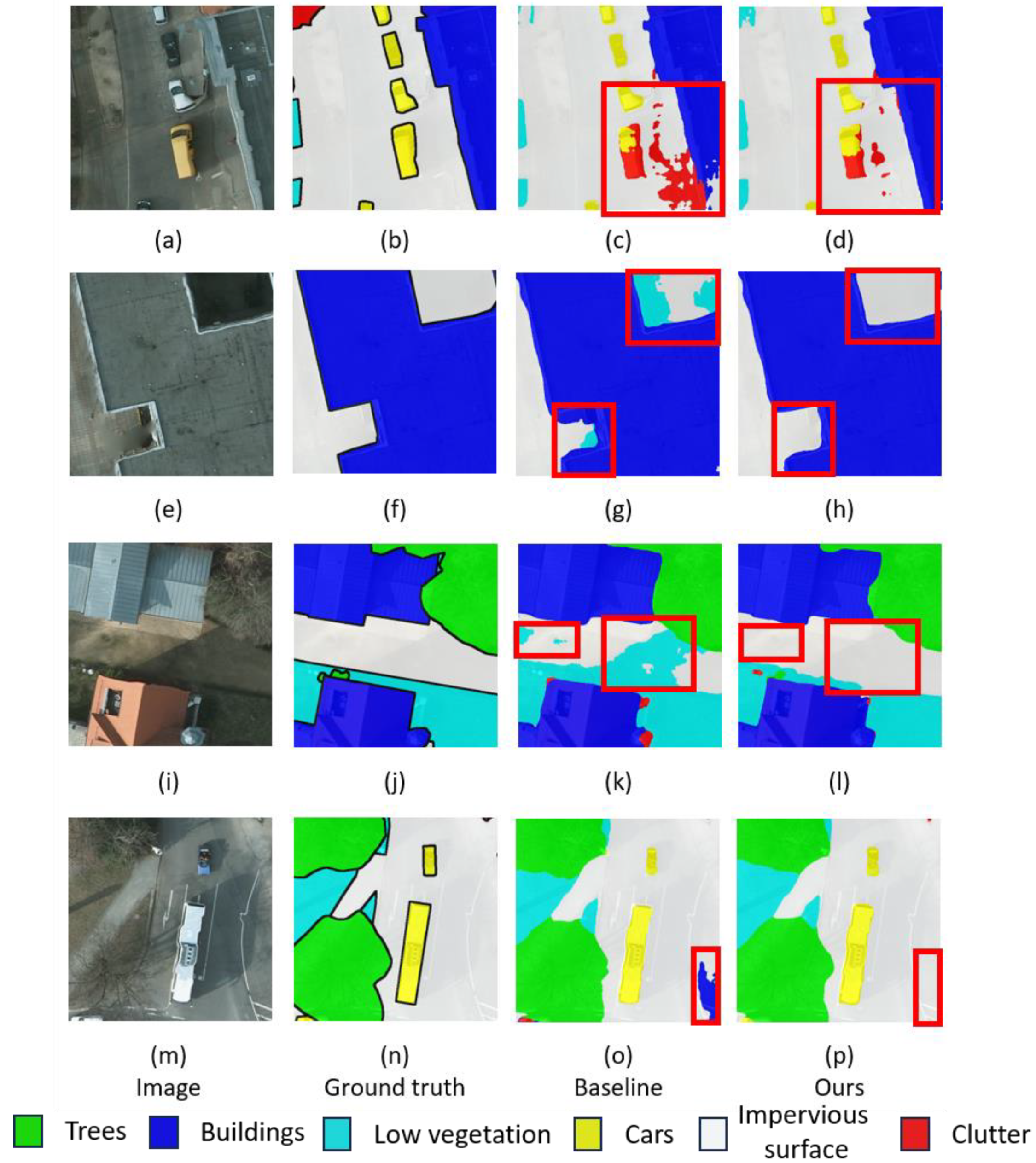
Figure 11 and
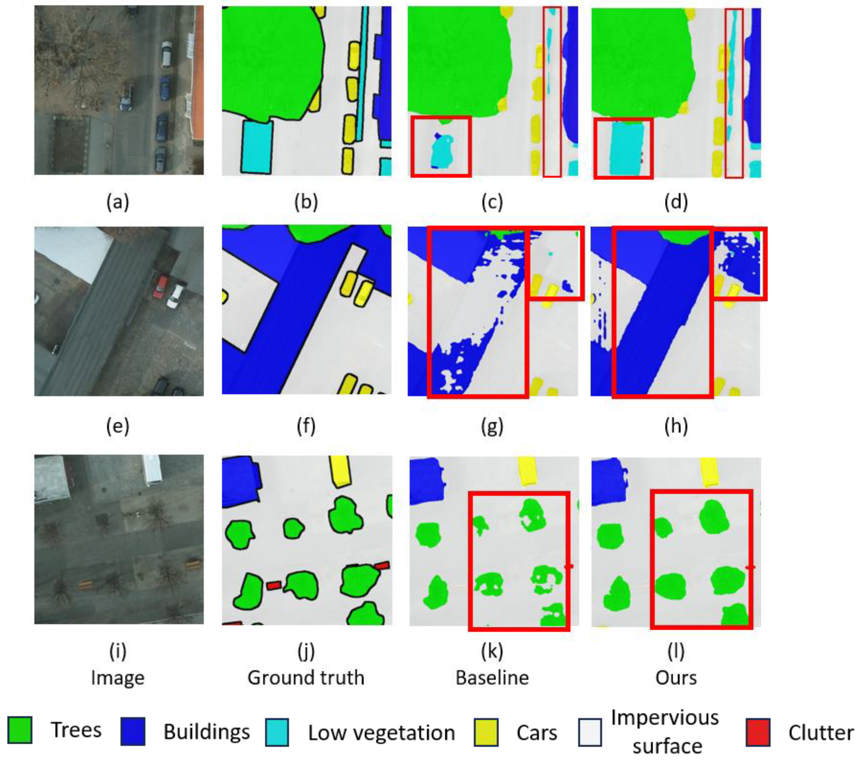
Figure 12 visually display how the two architectural configurations discussed in this paper enhance model segmentation precision.
The sections highlighted with red borders in
Figure 11 and
Figure 12 significantly demonstrate the substantial improvement in land-cover classification accuracy of the system integrated with the decoder we designed. It can be observed that, compared to the baseline segmentation results in the third column, the “ours” in the fourth column is closer to the ground truth in terms of segmentation results, thereby showing a distinct advantage. For instance, in the segmentation of
Figure 11a,e,i,m, the baseline incorrectly classifies the background as other categories, while our model avoids this issue, indicating that the attention modules we designed effectively reduce the interference of background noise. In
Figure 12a,e,i, the baseline incorrectly judges other categories as the background, while our model avoids this problem. This not only represents the classification of land-cover features on a small and large scale but also shows the enhancement of the model’s segmentation capabilities across different scales. These results highlight the system’s adaptability and flexibility in efficiently processing targets of various sizes.
4. Discussion
We have introduced a multi-dilated convolution fusion module and a large-kernel convolution hybrid attention module, dedicated to enhancing the performance of remote-sensing image segmentation. These designs have broadened the model’s receptive field, significantly enhancing the capability to capture global features and distinguish between the foreground and background. Notably, our improved method achieved remarkable improvements in key segmentation metrics such as mIoU and mF1.
These accomplishments are attributed to the innovative redesign of our decoder. As described in
Section 2, we integrated multi-dilated convolution fusion module and a convolutional kernel selection module into the decoder, effectively merging feature maps processed through multiple convolutional pathways, balancing the recognition capabilities for both large-scale and fine-scale targets. The strategy of dynamically selecting an appropriate receptive field within LKSHAM also played a crucial role in enhancing performance. At the same time, the expanded receptive field enhanced the model’s ability to perceive global features, thereby more effectively distinguishing between the foreground and background. The introduction of the hybrid attention mechanism and large-kernel convolution technology has further promoted improvements in performance. The effects of these improvements are intuitively demonstrated in
Figure 11 and
Figure 12.

