Article

SSANet-BS: Spectral–Spatial Cross-Dimensional Attention Network for Hyperspectral Band Selection

1
College of Computer Science and Technology, Qingdao University, Qingdao 266071, China
2
School of Information Science and Technology, Dalian Maritime University, Dalian 116026, China
*
Author to whom correspondence should be addressed.
Remote Sens. 2024, 16(15), 2848; https://doi.org/10.3390/rs16152848
Submission received: 27 May 2024 / Revised: 22 July 2024 / Accepted: 26 July 2024 / Published: 3 August 2024

Abstract

:
Band selection (BS) aims to reduce redundancy in hyperspectral imagery (HSI). Existing BS approaches typically model HSI only in a single dimension, either spectral or spatial, without exploring the interactions between different dimensions. To this end, we propose an unsupervised BS method based on a spectral–spatial cross-dimensional attention network, named SSANet-BS. This network is comprised of three stages: a band attention module (BAM) that employs an attention mechanism to adaptively identify and select highly significant bands; two parallel spectral–spatial attention modules (SSAMs), which fuse complex spectral–spatial structural information across dimensions in HSI; a multi-scale reconstruction network that learns spectral–spatial nonlinear dependencies in the SSAM-fusion image at various scales and guides the BAM weights to automatically converge to the target bands via backpropagation. The three-stage structure of SSANet-BS enables the BAM weights to fully represent the saliency of the bands, thereby valuable bands are obtained automatically. Experimental results on four real hyperspectral datasets demonstrate the effectiveness of SSANet-BS.

1. Introduction

Hyperspectral imagery (HSI) records numerous contiguous and narrow spectral bands, and has been extensively utilized in diverse fields such as military and industry [1]. Nonetheless, the high redundancy of bands in HSI poses great challenges in terms of data transmission, storage, and computation, and can also lead to the Hughes phenomenon in classification, thereby reducing classification accuracy [2,3]. Consequently, dimensionality reduction is essential for HSI.
The dimensionality reduction in HSI can be divided into two categories: feature extraction (FE) and band selection (BS) [4]. FE aims to project the original HSI into a lower-dimensional space, which results in the loss of HSI’s physical information due to alterations in the feature space. Conversely, BS focuses on selecting a representative band subset from HSI that preserves the physical significance and has higher interpretability, which is more preferable for practical applications [5,6,7].
According to different task scenarios, BS methods can be primarily categorized into target detection-oriented methods and classification-oriented methods. The former typically considers the spectral differences between targets and backgrounds when selecting a subset of bands [8,9], whereas the latter selects bands that contain a large amount of information and exhibit strong discrimination capability [10,11]. Most of these methods are supervised and depend on prior information, such as ground truth labels, which limits their practical application. In contrast, unsupervised methods do not rely on prior information, but select the representative bands by identifying the intrinsic properties of HSIdata. It is more versatile and can be applied to downstream tasks in all scenarios, including classification [12]. Hence, the focus of this paper is on unsupervised band selection methods which are more versatile for task scenarios.
The initial BS approaches employed the artificially designed band evaluation metrics or heuristic strategies to obtain target bands [1]. However, the manually designed BS process was unable to account for the complex real-world factors in a comprehensive manner, resulting in unsatisfactory performance. The advent of machine learning has offered novel insights into the field of BS. The maximum-variance principal component analysis (MVPCA) [13] and Boltzmann entropy-based band selection (BE) [14] employ specific metrics derived from machine learning models to evaluate the equality of bands. Techniques such as fast density-peak-based clustering (E-FDPC) [15] and graph regularized spatial–spectral subspace clustering (GRSC) [16] utilize clustering to partition bands into multiple clusters, from which the most representative band in each cluster is selected. The sparse representation-based band selection (SpaBS) [17] and spectral–spatial hypergraph-regularized self-representation (HyGSR) [18] operate under the assumption that the original HSI can be represented by a linear combination of a limited number of bands, identifying the optimal band combination through iterative optimization of the sparse representation model. Those above machine learning-based BS methods attained considerable performance and can effectively reduce band redundancy.
However, those BS methods usually rely on strong assumptions to model the internal interactions within HSI [19,20]. In reality, the interaction between bands and pixels is complex [21]. Due to various physical factors, the reflectance of band in a certain pixel is influenced by its surrounding pixels and bands. Thus, the predefined strong assumptions cannot cover all situations, and hence are not the optimal solution [22,23,24,25].
Neural networks possess remarkable fitting capabilities and can reveal the intricate interdependent relationships in HSI [26,27,28]. The attention mechanism is effective in distinguishing the important features [29,30]. Networks with the attention mechanism can automatically learn the potential interrelations and distinguish the most representative bands of HSI [31,32]. Therefore, various attention modules are widely employed in the field of band selection. On this basis, BS-Nets [33] is the first band selection framework that combines band attention mechanism and autoencoder. This model utilizes attention mechanism to search for important bands and applies band-wise attention weighting to the original HSI. By optimizing the model using an autoencoder, significant bands are selected according to the band attention weights.
Subsequently, various models have employed different attention mechanisms to model the spectral or spatial dimensions of HSI, and enhance the model performance. Attention-based autoencoder (AAE) [34] generates the attention mask for each pixel. Then, the band correlations are calculated based on the attention mask and the final band subset is obtained by clustering. Non-local band attention network (NBAN) [20] employs a global-local attention mechanism, which fully considers the nonlinear long-range dependencies of HSI in the band dimension. This approach significantly enhances the effectiveness and robustness of the attention mechanism, facilitating the automatic selection of bands. Dual-attention reconstruction network (DARecNet-BS) [35] incorporates two independent self-attention mechanisms, one in the spectral dimension and the other in the spatial dimension. These mechanisms enhance the results of band selection by exploring the dependencies of HSI in various dimensions.
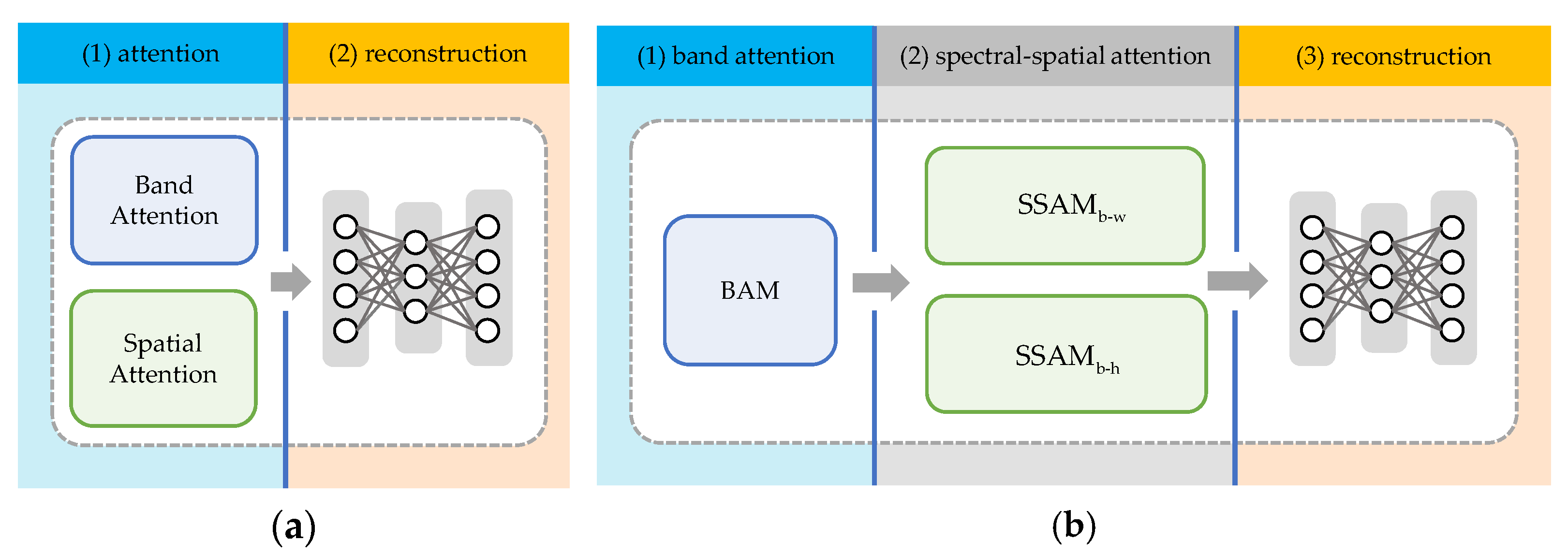
The aforementioned methods have utilized the nonlinear interaction information within HSI, yielding promising results. However, these methods solely model in the spectral or spatial dimensions independently, overlooking the potential improvement in performance achieved from considering the connections between them. Most of them are two-stage models, i.e., attention and reconstruction network, which brought new challenges. Methods such as DARecNet-BS and the triplet-attention and multi-scale reconstruction network (TAttMSRecNet) [36] introduce spatial attention modules connected in parallel with the band attention module to mine image spatial information, as shown in Figure 1a. The band attention module and the spatial attention modules are integrated to function in unison, thereby rendering the band attention weights unable to represent the saliency of the bands independently. Hence, these methods are incapable of selecting bands based on the converged band attention weights and must rely on calculating the entropy of the reconstructed image for band selection, a process that constrains the potential of the attention mechanism to automatically identify significant bands.
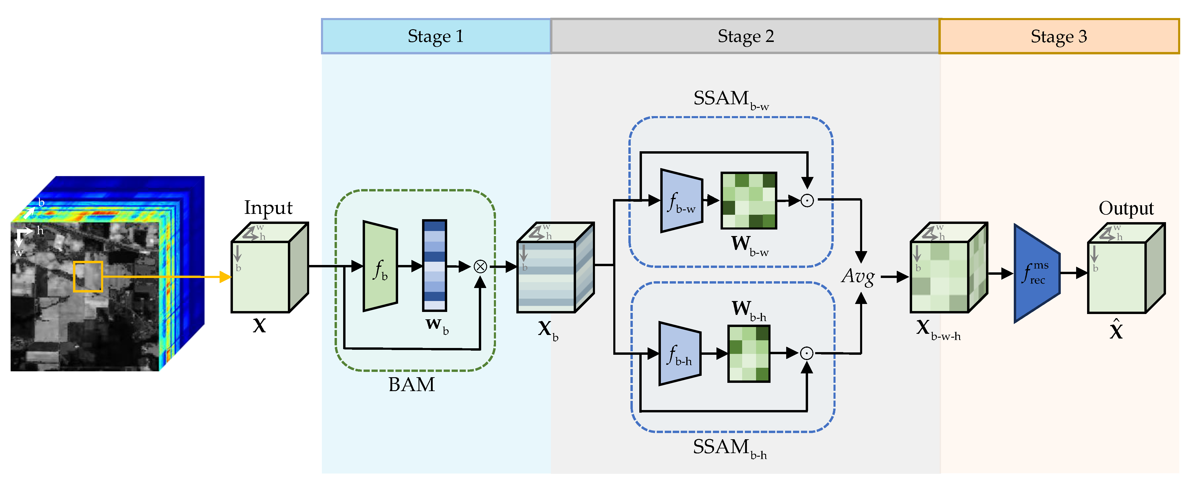
In this end, we propose a deep neural network, SSANet-BS, based on spectral–spatial cross-dimensional attention. SSANet-BS is a three-stage model, as shown in Figure 1b and Figure 2. This network regards BS as a reconstruction task for HSI to achieve unsupervised BS that is applicable to scenarios such as classification. Initially, a band attention module (BAM) is designed to model the spectral dimension of HSI, extracting salient band features, and outputting band attention weights. Subsequently, two spectral–spatial attention modules (SSAMs) are constructed in the band-width (b-w) and band-height (b-h) directions using the BAM-weighted image as input, to explore the complex spectral–spatial interactions within HSI, and generate SSAM weights along with SSAM-fused image. Finally, a multi-scale reconstruction network is used to reconstruct the above fused image. In the optimization process, the band attention weights obtained by BAM are gradually converged to the bands with large information and high saliency. Compared with the above two-stage methods, DARecNet-BS and TAttMSRecNet, SSANet-BS makes SSAMs compatible with BAM by the ingenious design of the three-stage structure, and fully takes advantage of the automatic convergence of the attention mechanism to the important bands during the back propagation process to achieve automatic band selection. The main contributions of this paper are as follows:
  • This paper proposes a deep neural network based on spectral–spatial cross-dimensional attention for hyperspectral BS, named SSANet-BS. This network employs complementary multi-dimensional attention mechanisms to automatically discover salient bands, and improves the performance of BS by exploring the complex spectral–spatial interactions in HSI.
  • SSANet-BS, with its three-stage structural design, addresses the issue of existing BS methods that introduce spatial modules, which compromise the independence of the band attention weights. The experimental results demonstrate that SSANet-BS is effective and stable. This offers a novel solution for the field of hyperspectral BS.

2. The Proposed Method

This section introduces the proposed method, SSANet-BS, outlines its design concept and overall structure, and presents the implementation details of every module and step.

2.1. Overview of SSANet-BS

SSANet-BS treats BS as a task of band-weighted reconstruction for HSI. To enhance performance, it fully models the nonlinear interactions between pixels and bands in HSI [37] throughout the reconstruction process. SSANet-BS is comprised of three stages, and the overall structure is shown in Figure 2.
In the first stage, SSANet-BS inputs image patch X M × N × L from the original HSI multiple times as a single input with width M, height N, and number of bands L. This process ensures that SSANet-BS can read the original HSI thoroughly. Afterwards, X is fed into the band attention module (BAM) to obtain band attention weights, which are then applied proportionally. The output of BAM is a band-attention-weighted image with enhanced salient bands.
The second stage is designed to extract the spectral–spatial information of the HSI. The above BAM-weighted image is input into two spectral–spatial attention modules (SSAMs) to fully explore the complex spectral–spatial cross-dimesional interactions. This leads to the generation of spectral–spatial attention weights, which are later used to construct the SSAM-fusion image.
The third stage is the reconstruction of the attention-weighted HSI for model optimization. A multi-scale reconstruction network based on 3D convolution and transposed convolution is employed to reconstruct the aforementioned SSAM-fusion image. The loss function is defined as the residual between the reconstructed image and the original image, facilitating the optimization of SSANet-BS.
It should be noted that the existing two-stage approach employs a band attention module and other modules in the same stage. Consequently, the band attention weights are unable to represent the salience of bands independently. In contrast, the BAM of SSANet-BS is employed independently in the first stage. Therefore, the weight vector generated by the BAM represent the salience or reconstruction capability of each band in relation to the original HSI. When SSANet-BS reaches convergence, the band attention weights are sorted in descending order. The higher the band ranking, the higher its priority. Specifically, the details of each module in SSANet-BS are illustrated below.

2.2. The Band Attention Module

The BAM takes X as input, and generates a band attention weight vector through neural network f b within this module:
w b = f b ( X )
The i-th element w b i [ 0 , 1 ] of the vector w b L represents the salience of the i-th band b i in X. A higher value of w b i indicates that b i contributes more to the reconstruction of X, making it more salient. The structure of f b is detailed in Figure 3 and Table 1. Compared to using a fully connected network to extract band information from a single pixel, employing a convolutional neural network with spatial inductive bias [33] can effectively make use of spatial information and boost modeling capabilities. Consequently, the initial layer of the network uses multiple 2D convolution kernels to extract band information, while the second layer employs max-pooling operations to reduce the feature dimension of the output of the convolutional layer. Finally, after passing through a fully connected network with a sigmoid activation function and batch normalization, the weight vector w b can be obtained.
Subsequently, X is weighted band-by-band to generate the output image X b of BAM:
X b = f linear ( w b ) X
Here, X b M × N × L . represents band-wise multiplication, and f linear denotes the linear transformation operation. The L 1 regularization is imposed on the loss function of SSANet-BS, which introduces a sparse constraint on w b in order to reduce the redundancy of the final band subset. Therefore, some elements in w b may be 0 or close to 0. At this point, if X b is obtained through w b X , it will inevitably lose some original band information, making it difficult for the subsequent SSAMs to fully model the spectral–spatial cross-dimensional interactions in HSI. Therefore, in this paper, the linear transformation f linear is adopted to map each element in w b from the range of [ 0 , 1 ] to [ 0.5 , 1 ] without changing relative relationship of band saliency. As the input of the subsequent module, X b enhances the features of salient bands in X, improving the rationality of BS.

2.3. The Spectral–Spatial Attention Module

If only a single dimension such as spectral or spatial considered in HSI reconstruction, the interdependent relationship between these dimensions is ignored. In reality, proper modeling of the complex nonlinear interactions in HSI can effectively improve the performance of model [36]. Based on this, SSANet-BS not only uses BAM to learn and model the interactions in the spectral dimension but also further introduces two spectral–spatial attention modules (SSAM) for the band-width (b-w) and band-height (b-h) directions. This approach aims at fusing the spectral–spatial information to deeply explore the complex spectral–spatial cross-dimensional dependencies in HSI.
SSAM b - w and SSAM b - h are implemented in the same way, except that the directions are different. Taking the SSAM b - w in b-w direction as an example, the neural network f b - w takes X b as input, and generates the spectral–spatial attention weight matrix W b - w in b-w direction:
W b - w = f b - w ( X b )
In Equation (3), the elements in W b - w M × L are non-negative. The detailed structure of f b - w is shown in Table 1. SSAM b - w first performs max-pooling and average-pooling along the height direction of X b to reduce its dimensionality, obtaining feature maps of salient and global information in the b-w direction. Further, by stacking the above two feature maps and passing them through a convolutional layer, a batch normalization layer and a ReLU nonlinear activation function, W b - w and the SSAM-weighted image of the b-w direction X b - w M × N × L can be obtained:
X b - w = W b - w X b
Here, represents the corresponding position-wise multiplication. Specifically, let X b - w k M × L and X b k M × L be the k-th section or layer of X b - w and X b in the height direction, 1 k L , respectively. Then, X b - w k is obtained by the element-wise multiplication of X b k and W b - w . Similarly, the module SSAM b - h outputs the SSAM-weighted image X b - h of the b-h direction. Then, X b - w and X b - h are fused to generate the SSAM-fusion image X b - w - h :
X b - w - h = A v g ( X b - w , X b - h )
In this case, A v g is the average operation. X b - w - h will provide spectral–spatial cross-dimensional interaction information for the adjustment of BAM weight vector w b and subsequent image reconstruction process, thus enabling SSANet-BS to fully utilize the spectral–spatial correlation information to select more reasonable bands and achieve performance improvement.

2.4. The Multi-Scale Reconstruction Network

3D convolutional networks can exploit spectral–spatial information and have found extensive usage in reconstructing HSI [36,38]. To develop a network that can model HSI’s interactions on varying scales and enhance reconstruction proficiency, this paper puts forth a multi-scale reconstruction network f rec ms inspired by MSRN [38] that incorporates 3D convolutions and transposed convolutions with diverse kernel scales. Then, the above SSAM-fusion image X b - w - h can be reconstructed by f rec ms :
X ^ = f rec ms ( X b - w - h )
The detailed implementation of f rec ms are displayed in Table 1. The SSAM-fusion image X b - w - h will be reconstructed as X ^ M × N × L using f rec ms . To ensure that bands with adjacent spectral positions are not assigned approximate attention weights and to reduce the redundancy of the band subset, the loss function of SSANet-BS is designed as:
J ( θ ) = 1 P X ^ X 2 + λ w b 1
Here, θ represents all trainable parameters of SSANet-BS. P = M × N denotes the total number of pixel in X. · 1 represents the L 1 sparse constraint. The coefficient λ controls the sparsity degree of w b . The three-stage design of SSANet-BS enables the band attention weight w b of the BAM to represent the band saliency independently, thus facilitating band selection. Specifically, the average of w b corresponding to each X, w ¯ b can be treated as the ultimate salience scores of each band once the SSANet-BS has converged. The larger the i-th atom of w ¯ b , the more important the i-th band b i . Based on this, after sorting the atoms of w ¯ b in descending order, the bands linked to the top n values are picked as the ultimate band subset.

3. Experiments

This section presents a comparative analysis of the proposed SSANet-BS model, two state-of-the-art feature extraction methods, and eight state-of-the-art BS methods on four publicly available datasets. The classification results are used to verify the effectiveness of each method. The experimental data, parameter settings, comprehensive analysis and discussions are detailed in the following sections.

3.1. Experimental Setup

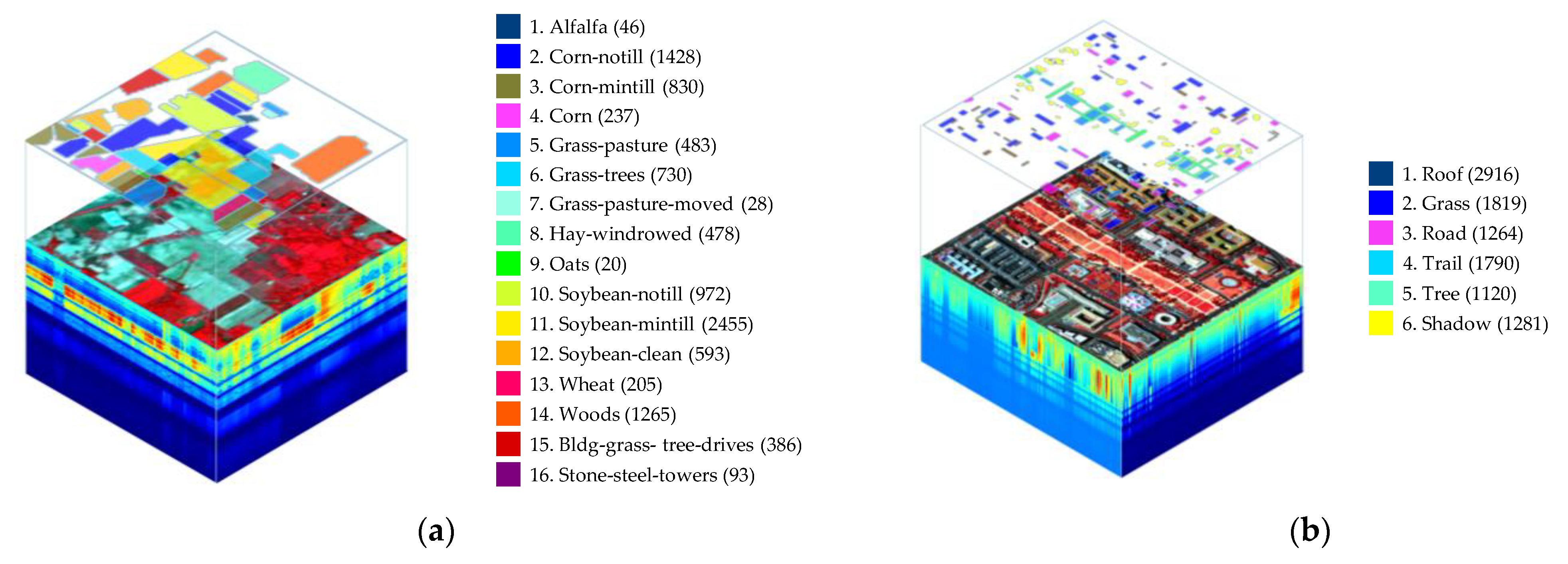
The comparison methods include locally linear embedding (LLE) [39], isometric mapping (Isomap) [40], maximum-variance principal component analysis (MVPCA) [13], enhanced fast density-peak clustering (E-FDPC) [15], adaptive subspace partitioning strategy (ASPS) [41], scalable one-pass self-representation learning (SOPSRL) [42], graph regularized spatial–spectral clustering (GRSC) [16], BSNet-Conv [33], DARecNet-BS [35] and spatial and spectral structure preserved self-representation ( S 4 P ) [43], respectively. It is crucial to emphasize that LLE and Isomap require significant computational resources for processing large-scale HSI. Therefore, sampled versions are chosen to ensure their successful operation on the four datasets. Further, in order to facilitate comparisons between the two feature extraction methods (LLE and Isomap) and the BS methods, the number of dimension after feature extraction is set equal to the number of selected bands. The four hyperspectral datasets are as follows, as shown in Figure 4:
  • Indian Pines (IP220): IP220 is captured by the AVIRIS sensor in 1992 in an Indian pine forest landscape which located at the northwest of Indiana. It contains 220 bands, with a resolution of 145 × 145 pixels and 16 classes of ground objects labeled.
  • Washington DC Mall (DC191): It is an airborne HSI acquired by the HYDICE sensor, which contains 191 bands, with a resolution of 280 × 307 and 6 classes.
  • Pavia University (PU103): PU103 is taken in 2002 by the ROSIS sensor in the campus of Pavia University in Italy. It size is 610 × 340 × 103, and has 9 classes.
  • QUH-Qingyun (QY176) [44]: The image was captured on 18 May 2021 in Qingdao, China, utilising a Gaiasky mini2-VN imaging spectrometer mounted on a UAV platform. It comprises 176 spectral bands. After cropping, it is 600 × 200 in size and contains 5 classes of ground labels.
The experiment uses Support Vector Machine (SVM) as the classifier, with 10%, 1%, 5%, and 10% samples selected from IP220, DC191, PU103 and QY176 for training. The classification results include producer’s accuracy (PA), average producer’s accuracy (APA), average user’s accuracy (AUA), overall accuracy (OA) and kappa coefficient (kappa) are used to assess the effectiveness of each method. To reduce the uncertainty caused by random sample selection, the OA of each band subset is the average from five independent tests. The experiment divides the HSI into multiple non-overlapping images X 7 × 7 × L as input for SSANet-BS, and takes the SGD as optimizer. SSANet-BS is implemented using the PyTorch framework based on CUDA 10.7. All experiments are run on Intel Xeon E5-2699 v4 CPU and Nvidia Tesla P40 GPU.

3.2. Parameter Setting

The hyperparameter of SSANet-BS, λ , is the coefficient to control the regularization. Its range is set to {0.0001, 0.001, 0.01, 0.1}. The optimal λ is determined based on the average OA (AOA) under the number of bands n BS varies from 5 to 30 with a step of 5. Table 2 shows the AOA values of SSANet-BS under different λ . It can be observed that the optimal values on the IP220, DC191, PU103 and QY176 datasets are 0.01, 0.0001, 0.001 and 0.0001, respectively.

3.3. Result Analysis

To validate the effectiveness of the proposed method, Figure 5 shows the OA values of five runs for each BS method at different n BS . For the IP220 dataset, SSANet-BS achieves the best results under most bands. It is closely followed by DARecNet-BS, GRSC, and ASPS, with E-FDPC, LLE and Isomap performing poorly. The advantage of SSANet-BS becomes more pronounced when fewer bands are selected. In terms of stability, the OA values of SSANet-BS, GRSC, and DARecNet-BS vary slightly under different n BS , while the OA values of ASPS drops when the n BS is 20, which is not stable. Meanwhile, Figure 5b reveals that SSANet-BS has a more significant advantage under most n BS on the DC191 dataset. As the n BS increases to 20, the gap between SSANet-BS and other comparison methods gradually narrows, still leaving SSANet-BS as an outstanding performer. For the PU103 dataset, although it is less effective than S 4 P when the n BS under 15, SSANet-BS still performs well. Nevertheless, it outperforms other methods in all other n BS . As with other datasets, SSANet-BS demonstrates an advantage over the other methods with fewer bands, such as 5 and 10, in the QY176 dataset. As the number of bands increase, the performance of SSANet-BS gradually approaches that of the other methods, with the exception of DARecNet-BS and MVPCA.
As shown in Figure 5, methods such as SSANet-BS, DARecNet-BS and S 4 P outperforms full bands across the majority of bands on the IP220 dataset. This indicates that those BS methods effectively reduced the data redundancy and further obtain good performance. On the DC191, PU103, and QY176 datasets, full bands surpasses all BS methods. However, as the number of bands increases, this gap gradually narrows. It is important to emphasize that the objective of BS is to improve data transmission and processing speed, conserve computational resources, and enhance model usability while maintaining task accuracy as much as possible. For instance, on the DC191 dataset with 191 bands, when the number of bands is 15, SSANet-BS achieves a reduction of approximately 92% in data volume with an 1.32% loss in OA. Moreover, in this experiment, the running time for SVM with 15 bands and full bands is 0.43s and 2.94s, respectively, which is of considerable importance in practical applications with large-scale datasets. Therefore, the BS methods incur a acceptable loss of accuracy to significantly reduce the data volume of HSI, thereby increasing processing efficiency.
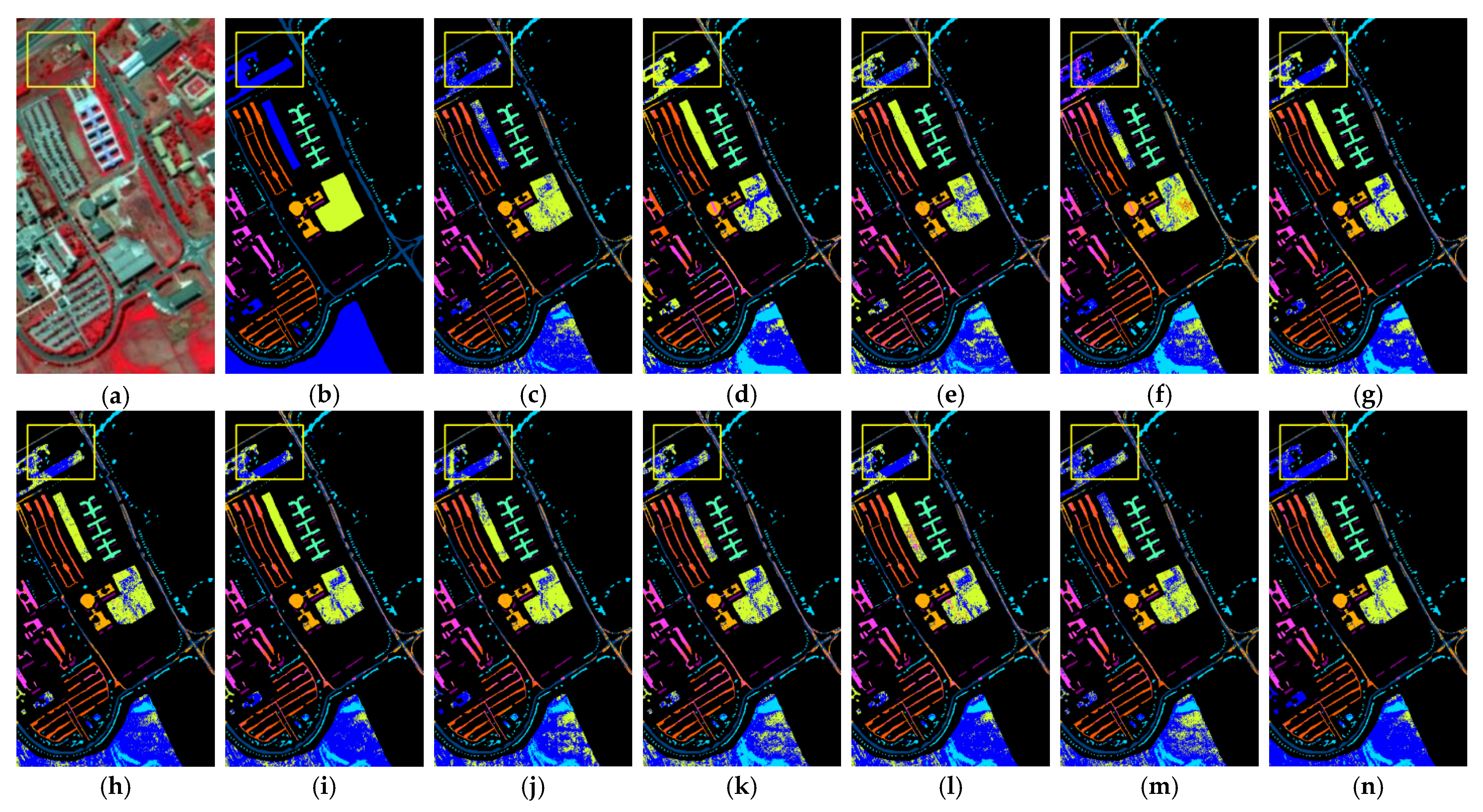
Further, Figure 6, Figure 7, Figure 8 and Figure 9 illustrate the classification maps of each method on four datasets at n BS = 15 . It can be observed that there are discrepancies between the false color image (a) and the ground truth (b) in Figure 6, Figure 7, Figure 8 and Figure 9. These differences are more pronounced in the areas highlighted by the yellow box in Figure 9. One of the reasons for these discrepancies is the interference from shadows, reflections, and other disturbances. Therefore, these factors are more conducive to validating and distinguishing the effectiveness of different band selection methods. The classification maps demonstrate that the selected bands of SSANet-BS are more closely aligned with the ground truth than those of other methods. The prediction accuracy of SSANet-BS is higher in adjacent regions belonging to the same class. This phenomenon is more pronounced in the yellow box labelled region of Figure 6, Figure 7, Figure 8 and Figure 9. For instance, on the IP220 dataset, the bands selected by SSANet-BS exhibit a lower misclassification rate in the yellow box labelled region, in contrast to MVPCA, E-FDPC and other methods, which exhibit higher rates. Similarly, on the QY176 dataset, SSANet- BS is the most closely aligned with the ground truth in the yellow box, whereas methods such as DARecNet-BS and MVPCA are less effective. This indicates that the joint spectral–spatial information of HSI has been fully utilized.
Furthermore, Table 3, Table 4, Table 5 and Table 6 also present the producer’s accuracy (PA), average producer’s accuracy (APA), average user’s accuracy (AUA), overall accuracy (OA) and kappa coefficient (kappa) for each method at n BS = 15 on the IP220, DC191, PU103, and QY176 datasets, respectively. For the IP220 dataset, SSANet-BS achieves the optimal APA, AUA, OA and kappa, and PA in 11 classes. In those classes where SSANet-BS did not achieve the optimal outcome, the PA value between the SSANet-BS and the optimal method is less than 3% except class 7 and 16. The performance of SSANet-BS on DC191 and QY176 are comparable to that of IP220. The APA, AUA, OA and kappa of SSANet-BS all represent the optimal values. This indicates that the selected subset of bands for SSANet-BS is of high quality and that the classification performance is stable. When considered collectively, SSANet-BS achieves the optimal values of APA, AUA, OA, and kappa on the remaining datasets, with the exception on PU103, which is outperformed by S 4 P . This indicates that SSANet-BS is a stable method and that the selected bands can effectively represent the original HSI.
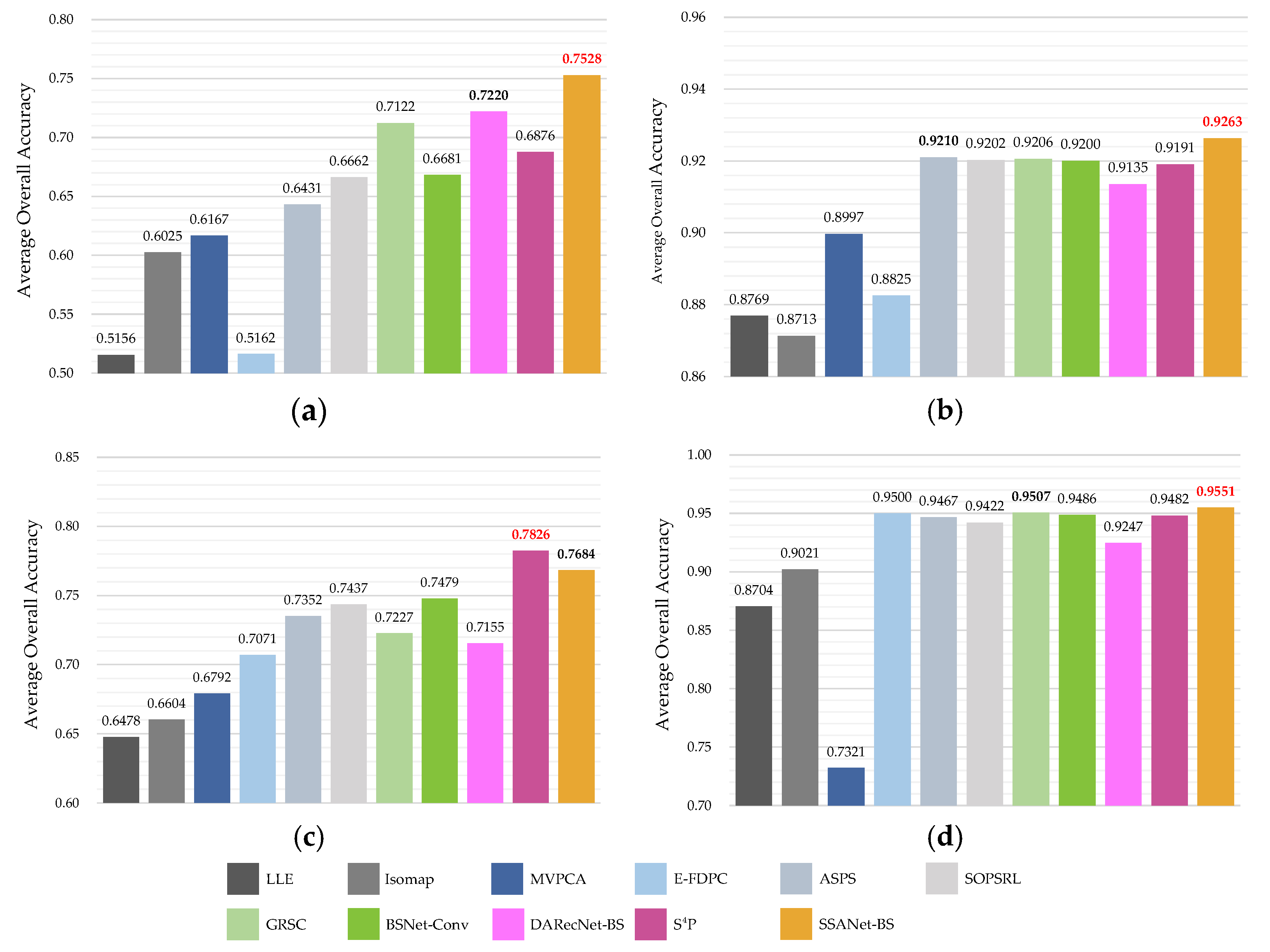
To further ensure the stability of SSANet-BS, Figure 10 presents the AOA values of each BS method across six band subset subgroups ranging from 5 to 30 with a step size of 5. The AOA values of the optimal and suboptimal methods are bolded in red and black. Upon examination of Figure 10, it is observed that there exists significant discrepancy in the performance of the various methods on the IP220 and PU103 dataset, whereas a relatively minor difference is noted on the DC191 and QY176 dataset. Moreover, most methods demonstrate superior performance on DC191 and QY176. This phenomenon can be attributed to a variety of factors, including sensor characteristics, the attributes of the ground objects within the scenes, atmospheric conditions, and the impact of lighting, among others. Consequently, the IP220 and PU103 present greater challenges for different BS methods. Figure 10 shows that the AOA values of SSANet-BS exceed those of all other comparison methods on the IP220, DC191 and QY176 datasets, leading the suboptimal methods by 3.08%, 2.05% and 0.44%, respectively. On the PU103 dataset, SSANet-BS is suboptimal, with a difference of only 1.42% from S 4 P but a 2.05% improvement over the third-best method BSNet-Conv. These outcomes indicate that SSANet-BS produces good and stable performance on various datasets by modeling complex spectral–spatial cross-dimensional interactions in the reconstruction process.

4. Discussion

This section discusses the quality of the selected band subset and the runtime of each method, verifies the effectiveness of two SSAM modules through ablation experiments, and concludes with the advantages and limitations of SSANet-BS.

4.1. Band Quanlity

Hyperspectral band selection methods aim to select a subset of bands that are both informative and low-redundancy, while also providing a comprehensive representation of the original HSI. Consequently, the quantity of information and the degree of redundancy are pivotal metrics for evaluating the quality of the band subset selected by the BS method under examination. On the one hand, bands with greater information content exhibit higher Shannon entropy values. On the other hand, the content of adjacent bands in HSI is similar and tends to be redundant [44], which means that the distribution of bands can reflect the redundancy of the band subsets.
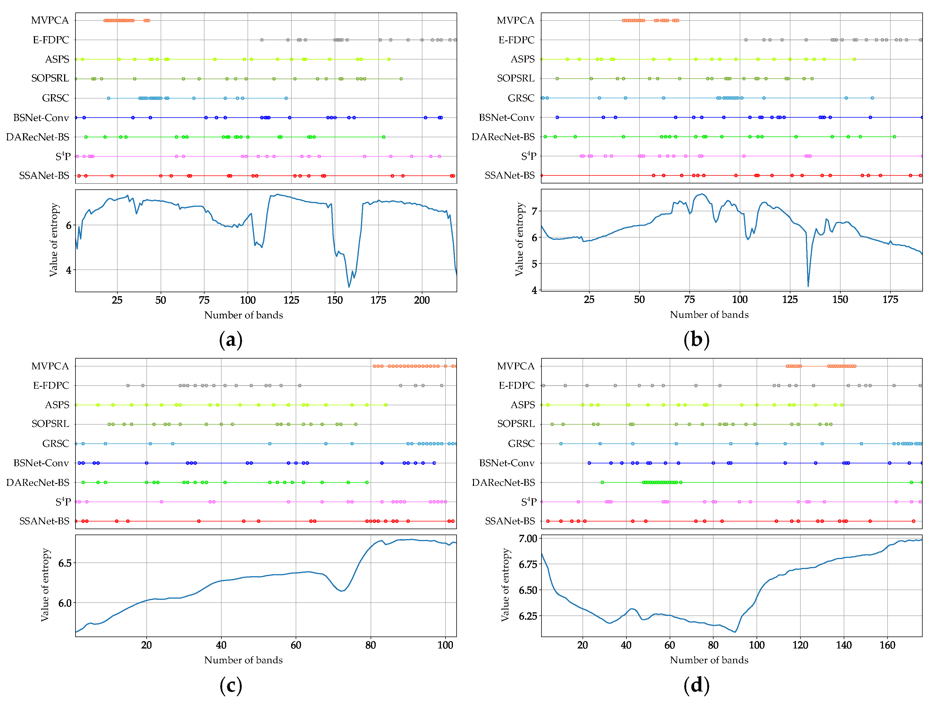
It can be observed in Figure 11 that bands with high entropy exhibit greater clarity in the features of ground objects. Conversely, bands with low entropy, such as Figure 11c, are noisy bands, which can have a detrimental impact on subsequent classification tasks. In order to assess the quality of the selected band for each method, Figure 12 further plots the distribution of the selected bands (top for each subplot), and the entropy values for all bands (bottom for each subplot) for the IP220 dataset. All subplots of Figure 12 indicates that the distribution of selected bands for MVPCA is concentrated in comparison to other methods. Although the selected bands of MVPCA are concentrated in the region of higher entropy, the classification performance is unsatisfactory. In contrast, methods such as EFDPC, ASPS, SOPSRL, BSNet-Conv and S 4 P , select bands that exhibit greater dispersion but inevitably fall within the low entropy range. The sparse constraints imposed on SSANet-BS result in a uniform distribution of bands across the four datasets. The selected bands are spaced further apart with lower redundancy and superior quality. This demonstrates the effectiveness of SSANet-BS.

4.2. Computation Time

This section mainly focuses on the computation time of SSANet-BS. Deep learning-based methods can be accelerated by GPU, so SSANet-BS, DARecNet-BS, and BSNet-Conv run on GPU, while the others run on CPU. Table 7 shows the computation time of different methods for selecting 30 bands on the IP220 dataset. Compared to other methods, deep learning-based methods take more time. Among the three deep learning methods, DARecNet-BS requires a significantly longer processing time than BSNet-Conv and SSANet-BS. The reason is that the band attention weights of DARecNet-BS can not represent the band saliency in its entirety. Consequently, DARecNet-BS is only able to select bands by calculating the entropy of the reconstructed image, which introduces additional computational cost. This disadvantage becomes more pronounced as the image size increases. Conversely, the three-stage structure of SSANet-BS enables the selection of bands from the converged band attention weights directly as in BSNet-Conv, thereby reducing the computational costs. This represents a distinct advantage of the three-stage structure of SSANet-BS.

4.3. Ablation Study for SSAMs

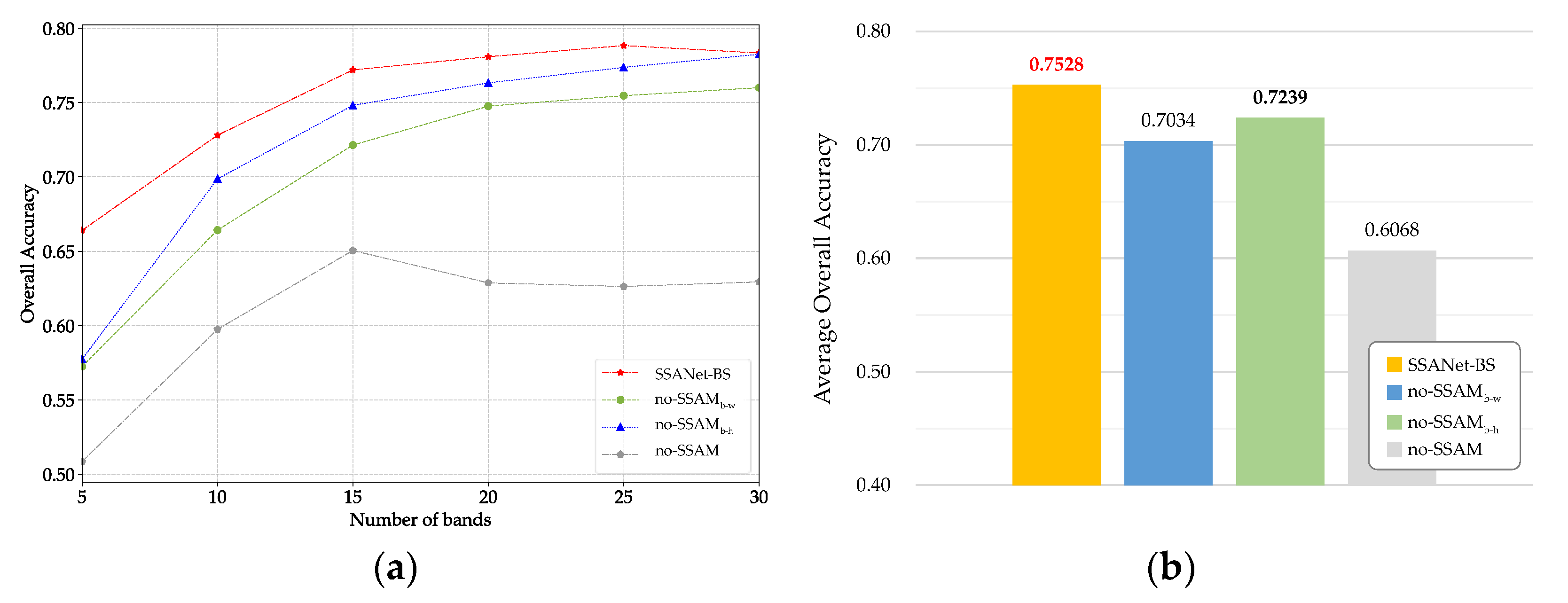
In this section, three variants of the SSANet-BS model are constructed to verify the effectiveness of SSAM. This is achieved by removing the SSAM b - w in the band-width (b-w) direction, SSAM b - h in band-height (b-h) direction and both of them in the SSANet-BS, respectively. The three aforementioned variants, designated as no - SSAM b - w , no - SSAM b - h , and no-SSAM, are subjected to testing on the IP220 dataset. The OA and A OA values of SSANet-BS, along with its three variants under n BS ranging from 5 to 30 are recorded, as shown in Figure 13.
As can be seen in Figure 13a, the SSANet-BS exceeds the three variants mentioned above at all n BS . Meanwhile, both variants lacking SSAM module in one direction, namely no - SSAM b - w and no - SSAM b - h , are superior to the variant without any SSAM module. In addition, the AOA values shown in Figure 13b indicate that in comparison to the complete SSANet-BS, the variants lacking either any modules SSAM b - w or SSAM b - h , SSAM b - h , or all modules exhibited a reduction in AOA values of 2.89%, 4.94% and 14.59%, respectively. Therefore, both SSAM b - w and SSAM b - h developed in this paper can effectively improve the model’s performance. The ablation study indicates that SSANet-BS has successfully utilized SSAM to capture the spectral–spatial information of HSI during the band selection process. The three-stage structure of SSANet-BS, comprising BAM, SSAMs and reconstruction network, has been demonstrated to be effective.

4.4. Effectiveness of the Three-Stage Structure

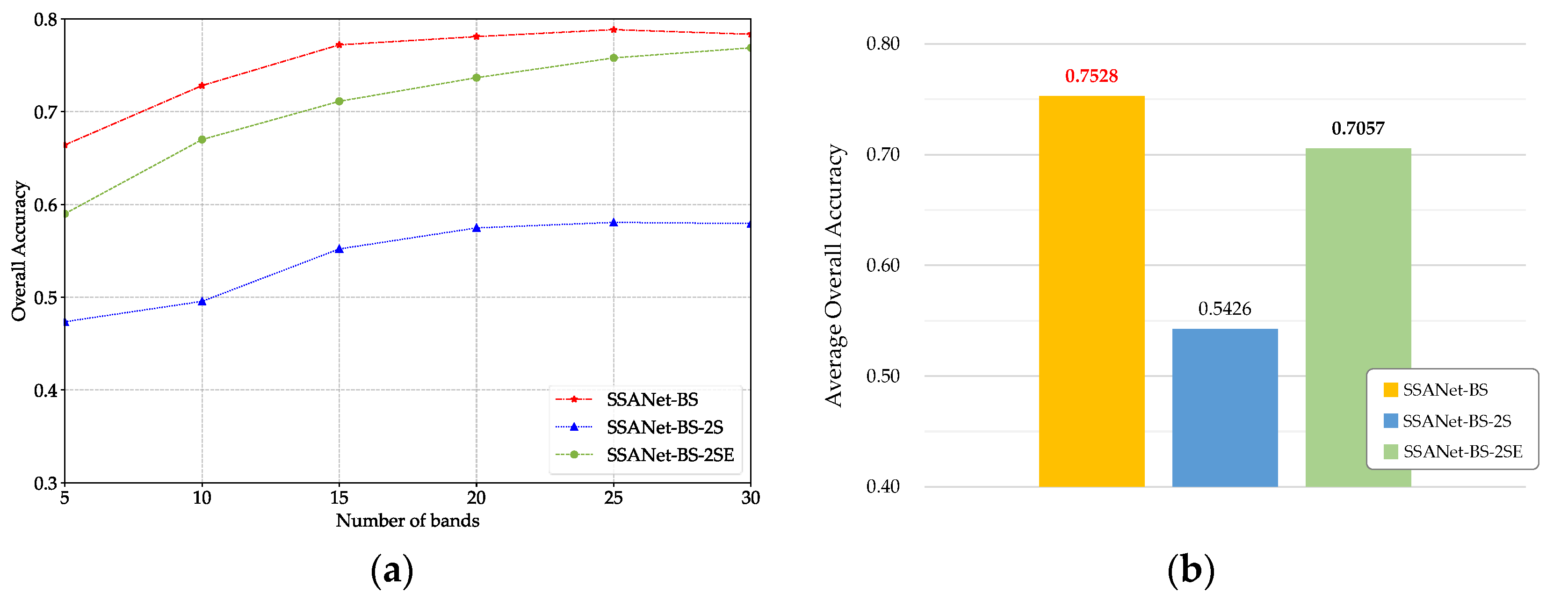
In order to validate the necessity and effectiveness of the three-stage structure, a variant of the SSANet-BS with two-stage has been constructed. This variant is named SSANet-BS-2S. In SSANet-BS-2S, the BAM is situated in the same stage as the two SSAMs, which are in a parallel relationship. This is in contrast to the progressive relationship in the three-stage version of SSANet-BS.
Under the optimal parameters, Figure 14 shows that the performance of SSANet-BS-2S is markedly inferior to that of SSANet-BS, exhibiting an approximate 21% deficit in AOA. The discrepancy can be attributed to the fact that, in the variant SSANet-BS-2S which is a two-stage structure, the BAM and the two SSAMs operate in a cooperative manner, jointly modelling the HSI. Information pertaining to the significance of bands is distributed throughout the hidden features of w b , W b - w , and W b - h . Consequently, w b cannot independently and comprehensively represent the significance of bands. In contrast, within the SSANet-BS which is a three-stage structure, the BAM and SSAMs are in a progressive order. The spectral–spatial information within HSI learned by the SSAMs is used to guide the adjustment of wb in the BAM via backpropagation, enabling w b to automatically converge to the bands with high significance during the training process.
To further validate the effectiveness of the three-stage structure of SSANet-BS, we developed a variant based on SSANet-BS-2S, termed SSANet-BS-2SE. In order to address the aforementioned issues that have arisen from the introduction of spatial or spectral–spatial modules, DARecNet-BS selects bands with higher entropy value during the reconstructed process. Variant SSANet-BS-2SE implements band selection in an analogous manner. Figure 14 illustrates that SSANet-BS-2SE demonstrates a notable enhancement in performance relative to SSANet-BS-2S. Nevertheless, it still exhibits a performance deficit when compared to SSANet-BS. This suggests that, in comparison to criteria (entropy) that have been manually designed, the automatic discovery of salient bands using attention mechanisms can effectively enhance model performance. It is evident that the two-stage structure of SSANet-BS-2SE is unable to fully capitalize on the advantages of the attention mechanism.
In conclusion, the three-stage structure of SSANet-BS guarantees that the band attention weights can independently and comprehensively represent the significance of bands. This allows the attention mechanism to automatically evaluate and select salient bands and achieve superior results. Therefore, the three-stage structure is both an effective and necessary.

4.5. Comments on Existing BS Methods and SSANet-BS

The attention mechanism can be used to learn the complex spectral–spatial interactions within HSI and enable the automated identification of significant bands. Current research on deep learning-based BS methods predominantly focuses on how to more effectively utilize attention mechanisms to enhance model performance. BS-Net [33] is the first BS method to automatically select bands using an attention mechanism. Then, NBAN [20] employs a non-local attention mechanism to capture long-range contextual information in the spectral dimension. Next, DARecNet-BS [35] introduces an independent spatial attention module and TAttMSRecNet [36] further exploits spectral–spatial information to improve model performance. By contrast, the proposed method SSANet-BS makes the SSAMs compatible with the BAM through the ingenious design of the three-stage structure, and achieves automatic band selection using the attention mechanism based on the full use of spectral–spatial information. The experimental results demonstrate that SSANet-BS is an effective and stable method.
BSNet-Conv is characterized by a straightforward structure that facilitates expeditious processing in real-world scenarios. Nonetheless, Its performance is generally mediocre. DARecNet-BS incorporates an independent spatial attention module, which offers new insights for HSI BS domain. However, the band selection process of DARecNet-BS relies on entropy, which results in a slower processing speed. SSANet-BS achieves promising results by learning the spectral–spatial information of HSIs. But according to statistics from the PyTorch framework, for the IP220 dataset (comprising 220 bands), the parameter count of SSANet-BS is about 43% higher than that of BSNet-Conv. The augmented number of parameters results in a greater requirement for GPU memory. This is less conducive to computing platforms with lower specifications, which may limit its applicability in certain contexts. However, in the context of today’s highly developed GPU hardware, the parameter volume of SSANet-BS does not present a significant bottleneck in application. With the rapid advancement of computer technology, this disadvantage is becoming mitigated.
Further, deep learning-based methods, including SSANet-BS, have the following potential issues. In contrast to domains such as CV and NLP, where models are employed in the manner of inference [45,46], the band selection process of existing attention-based BS methods is conducted on the training process. The existing BS model can only learn information about the target HSI, which greatly limits the potential capability of the neural network. In addition, due to the training process, the deep learning-based BS method takes tens or even hundreds of times longer than machine learning-based methods. Therefore, it is interesting to see how to make the model train on multiple HSIs, and implement BS on target HSI in the manner of inference. The inference process of neural network is much faster than the training process, and if the training can be done on multiple HSIs, it may be possible to obtain a BS method with higher performance and comparable time to machine learning-based methods. In the future, we will fully study those above issues and improve SSANet-BS.
5. Conclusions

This paper presents SSANet-BS, a network designed for BS. SSANet-BS is a three-stage BS method that solves the problem that existing two-stage BS methods cannot automatically search for salient bands using the attention mechanism while learning spatial information. It considers BS as a weighted reconstruction task of HSI, and leverages BAM and SSAMs to model the complex spectral–spatial cross-dimensional nonlinear interactions in HSI during the reconstruction process. Further, a multi-scale reconstruction network, featuring convolution kernels of various scales, is used to reconstruct HSI to optimize model. Experimental results on four publicly available datasets demonstrate that SSANet-BS outperforms existing BS methods and exhibits satisfactory stability. In the future, SSANet-BS is expected to be deployed and utilized for tasks including HSI classification, segmentation, and target detection, providing strong support for the HSI processing field.

Author Contributions

Conceptualization, X.S. (Xiaodi Shang); methodology, C.C. and X.S. (Xiaodi Shang); software, C.C. and X.S. (Xiaodi Shang); validation, C.C.; formal analysis, C.C.; investigation, C.C.; resources, C.C.; data curation, B.F.; writing—original draft preparation, C.C.; writing—review and editing, X.S. (Xiaodi Shang) and X.S. (Xudong Sun); visualization, C.C. and X.S. (Xudong Sun); supervision, X.S. (Xiaodi Shang) and X.S. (Xudong Sun); project administration X.S. (Xiaodi Shang); funding acquisition, X.S. (Xiaodi Shang). All authors have read and agreed to the published version of the manuscript.

Funding

This work was supported in part by Qingdao Natural Science Foundation Grant 23-2-1-64-zyyd-jch, in part by China Postdoctoral Science Foundation Grant 2023M731843, in part by the Postdoctoral Applied Research Foundation of Qingdao under Grant QDBSH20230101012, in part by the National Natural Science Foundation of China under Grant 42301380, and in part by the Science and Technology Support Plan for Youth Innovation of Colleges and Universities of Shandong Province of China under Grant 2023KJ232. (Corresponding author: Xiaodi Shang).

Data Availability Statement

The dataset utilized in this text can be accessed at the following links. IP220 (Indian Pines) and PU103 (Pavia University): https://www.ehu.eus/ccwintco/index.php/Hyperspectral_Remote_Sensing_Scenes (accessed on 24 May 2024). DC191 (Washington DC Mall): https://www.researchgate.net/figure/Washington-DC-Mall-HSI-a-Red-band-63-Green-band-50-and-Blue-band-27-sample-image_fig5_342993074 (accessed on 24 May 2024). QY176 (QUH-Qingyun): https://github.com/RsAI-lab/QUH-classification-dataset (accessed on 24 May 2024).

Conflicts of Interest

The authors declare no conflicts of interest.

References

  1. Sun, W.; Du, Q. Hyperspectral Band Selection: A Review. IEEE Geosci. Remote Sens. Mag. 2019, 7, 118–139. [Google Scholar] [CrossRef]
  2. Sun, X.; Lin, P.; Shang, X.; Pang, H.; Fu, X. MOBS-TD: Multiobjective Band Selection with Ideal Solution Optimization Strategy for Hyperspectral Target Detection. IEEE J. Sel. Top. Appl. Earth Obs. Remote Sens. 2024, 17, 10032–10050. [Google Scholar] [CrossRef]
  3. Li, Q.; Wang, Q.; Li, X. An Efficient Clustering Method for Hyperspectral Optimal Band Selection via Shared Nearest Neighbor. Remote Sens. 2019, 11, 350. [Google Scholar] [CrossRef]
  4. Vaddi, R.; Manoharan, P. CNN Based Hyperspectral Image Classification Using Unsupervised Band Selection and Structure-Preserving Spatial Features. Infrared Phys. Technol. 2020, 110, 103457. [Google Scholar] [CrossRef]
  5. Deep, K.; Thakur, M. Hyperspectral Band Selection Using a Decomposition Based Multiobjective Wrapper Approach. Infrared Phys. Technol. 2024, 136, 105053. [Google Scholar] [CrossRef]
  6. Fu, B.; Sun, X.; Cui, C.; Zhang, J.; Shang, X. Structure-Preserved and Weakly Redundant Band Selection for Hyperspectral Imagery. IEEE J. Sel. Top. Appl. Earth Obs. Remote Sens. 2024, 1–15, Early access. [Google Scholar] [CrossRef]
  7. Li, S.; Wang, Z.; Fang, L.; Li, Q. An Efficient Subspace Partition Method Using Curve Fitting for Hyperspectral Band Selection. IEEE Geosci. Remote Sens. Lett. 2024, 21, 1–5. [Google Scholar] [CrossRef]
  8. Gao, H.; Zhang, Y.; Chen, Z.; Xu, S.; Hong, D.; Zhang, B. A Multidepth and Multibranch Network for Hyperspectral Target Detection Based on Band Selection. IEEE Trans. Geosci. Remote Sens. 2023, 61, 1–18. [Google Scholar] [CrossRef]
  9. Song, M.; Liu, S.; Xu, D.; Yu, H. Multiobjective Optimization-Based Hyperspectral Band Selection for Target Detection. IEEE Trans. Geosci. Remote Sens. 2022, 60, 1–22. [Google Scholar] [CrossRef]
  10. Ou, X.; Wu, M.; Tu, B.; Zhang, G.; Li, W. Multi-Objective Unsupervised Band Selection Method for Hyperspectral Images Classification. IEEE Trans. Image Process. 2023, 32, 1952–1965. [Google Scholar] [CrossRef]
  11. Fu, H.; Zhang, A.; Sun, G.; Ren, R.; Jia, X.; Pan, Z.; Ma, H. A Novel Band Selection and Spatial Noise Reduction Method for Hyperspectral Image Classification. IEEE Trans. Geosci. Remote Sens. 2022, 60, 1–13. [Google Scholar] [CrossRef]
  12. Ji, L.; Zhu, L.; Wang, L.; Xi, Y.; Yu, K.; Geng, X. FastVGBS: A Fast Version of the Volume-Gradient-Based Band Selection Method for Hyperspectral Imagery. IEEE Geosci. Remote Sens. Lett. 2021, 18, 514–517. [Google Scholar] [CrossRef]
  13. Chang, C.; Du, Q.; Sun, T.; Althouse, M. A joint band prioritization and band-decorrelation approach to band selection for hyperspectral image classification. IEEE Trans. Geosci. Remote Sens. 1999, 37, 2631–2641. [Google Scholar] [CrossRef]
  14. Gao, P.; Wang, J.; Zhang, H.; Li, Z. Boltzmann Entropy-Based Unsupervised Band Selection for Hyperspectral Image Classification. IEEE Geosci. Remote Sens. Lett. 2019, 16, 462–466. [Google Scholar] [CrossRef]
  15. Jia, S.; Tang, G.; Zhu, J.; Li, Q. A Novel Ranking-Based Clustering Approach for Hyperspectral Band Selection. IEEE Trans. Geosci. Remote Sens. 2016, 54, 88–102. [Google Scholar] [CrossRef]
  16. Wang, J.; Tang, C.; Zheng, X.; Liu, X.; Zhang, W.; Zhu, E. Graph Regularized Spatial-Spectral Subspace Clustering for Hyperspectral Band Selection. Neural Netw. 2022, 153, 292–302. [Google Scholar] [CrossRef] [PubMed]
  17. Li, S.; Qi, H. Sparse Representation Based Band Selection for Hyperspectral Images. In Proceedings of the 18th IEEE International Conference on Image Processing, Brussels, Belgium, 11–14 September 2011; pp. 2693–2696. [Google Scholar]
  18. Shang, X.; Cui, C.; Sun, X. Spectral-Spatial Hypergraph-Regularized Self-Representation for Hyperspectral Band Selection. IEEE Geosci. Remote Sens. Lett. 2023, 20, 5504405. [Google Scholar] [CrossRef]
  19. Liu, Y.; Li, X.; Xu, Z.; Hua, Z. BSFormer: Transformer-Based Reconstruction Network for Hyperspectral Band Selection. IEEE Geosci. Remote Sens. Lett. 2023, 20, 5507305. [Google Scholar] [CrossRef]
  20. Li, T.; Cai, Y.; Cai, Z.; Liu, X.; Hu, Q. Nonlocal Band Attention Network for Hyperspectral Image Band Selection. IEEE J. Sel. Top. Appl. Earth Observ. Remote Sens. 2021, 14, 3462–3474. [Google Scholar] [CrossRef]
  21. Wang, M.; Liu, W.; Chen, M.; Huang, X.; Han, W. A Band Selection Approach Based on a Modified Gray Wolf Optimizer and Weight Updating of Bands for Hyperspectral Image. Appl. Soft Comput. 2021, 112, 107805. [Google Scholar] [CrossRef]
  22. Yao, Q.; Zhou, Y.; Tang, C.; Xiang, W.; Zheng, G. End-to-End Hyperspectral Image Change Detection Based on Band Selection. IEEE Trans. Geosci. Remote Sens. 2024, 62, 1–14. [Google Scholar] [CrossRef]
  23. Feng, J.; Bai, G.; Li, D.; Zhang, X.; Shang, R.; Jiao, L. MR-Selection: A Meta-Reinforcement Learning Approach for Zero-Shot Hyperspectral Band Selection. IEEE Trans. Geosci. Remote Sens. 2023, 61, 1–20. [Google Scholar] [CrossRef]
  24. Sun, W.; He, K.; Yang, G.; Peng, J.; Ren, K.; Li, J. A Cross-Scene Self-Representative Network for Hyperspectral Band Selection. IEEE Trans. Geosci. Remote Sens. 2024, 62, 5509212. [Google Scholar] [CrossRef]
  25. Amoako, P.Y.O.; Cao, G.; Yang, D.; Amoah, L.; Wang, Y.; Yu, Q. A Metareinforcement-Learning-Based Hyperspectral Image Classification with a Small Sample Set. IEEE J-STARS. 2024, 17, 3091–3107. [Google Scholar] [CrossRef]
  26. Hong, D.; Han, Z.; Yao, J.; Gao, L.; Zhang, B.; Plaza, A.; Chanusso, J. SpectralFormer: Rethinking Hyperspectral Image Classification with Transformers. IEEE Trans. Geosci. Remote Sens. 2022, 60, 1–15. [Google Scholar] [CrossRef]
  27. Zhang, H.; Sun, X.; Zhu, Y.; Xu, F.; Fu, X. A Global-Local Spectral Weight Network Based on Attention for Hyperspectral Band Selection. IEEE Geosci. Remote Sens. Lett. 2022, 19, 1–5. [Google Scholar] [CrossRef]
  28. Yang, J.; Zhou, J.; Wang, J.; Tian, H.; Liew, A. LiDAR-Guided Cross-Attention Fusion for Hyperspectral Band Selection and Image Classification. IEEE Trans. Geosci. Remote Sens. 2024, 62, 5515815. [Google Scholar] [CrossRef]
  29. Liu, Z.; Lin, Y.Z.; Cao, Y.Z.; Hu, H.; Wei, Y.; Zhang, Z.; Lin, S.; Guo, B. Swin transformer: Hierarchical vision transformer using shifted windows. In Proceedings of the IEEE/CVF International Conference on Computer Vision, Montreal, BC, Canada, 11–17 October 2021; pp. 9992–10002. [Google Scholar]
  30. Gao, L.; Chen, L.; Liu, P.; Jiang, Y.; Xie, W.; Li, Y. A Transformer-Based Network for Hyperspectral Object Tracking. IEEE Trans. Geosci. Remote Sens. 2023, 61, 1–11. [Google Scholar] [CrossRef]
  31. Zhang, H.; Gao, H.; Sun, H.; Sun, X.; Zhang, B. A Spatial-Spectrum Fully Attention Network for Band Selection of Hyperspectral Images. IEEE Geosci. Remote Sens. Lett. 2024, 21, 1–5. [Google Scholar] [CrossRef]
  32. Li, S.; Wang, M.; Cheng, C.; Gao, X.; Ye, Z.; Liu, W. Spectral-Spatial-Sensorial Attention Network with Controllable Factors for Hyperspectral Image Classification. Remote Sens. 2024, 16, 1253. [Google Scholar] [CrossRef]
  33. Cai, Y.; Liu, X.; Cai, Z. BS-nets: An End-to-End Framework for Band Selection of Hyperspectral Image. IEEE Trans. Geosci. Remote Sens. 2020, 58, 1969–1984. [Google Scholar] [CrossRef]
  34. Dou, Z.; Gao, K.; Zhang, X.; Wang, H.; Han, L. Band Selection of Hyperspectral Images Using Attention-Based Autoencoders. IEEE Geosci. Remote Sens. Lett. 2021, 18, 147–151. [Google Scholar] [CrossRef]
  35. Roy, S.K.; Das, S.; Song, T.; Chanda, B. DARecNet-BS: Unsupervised Dual-Attention Reconstruction Network for Hyperspectral Band Selection. IEEE Geosci. Remote Sens. Lett. 2021, 18, 2152–2156. [Google Scholar] [CrossRef]
  36. Nandi, U.; Roy, S.; Hong, D.; Wu, X.; Chanussot, J. TAttMSRecNet:Triplet-Attention and Multiscale Reconstruction Network for Band Selection in Hyperspectral Images. Expert Syst. Appl. 2023, 212, 118797. [Google Scholar] [CrossRef]
  37. He, K.; Sun, W.; Yang, G.; Meng, X.; Ren, K.; Peng, J.; Du, Q. A Dual Global–Local Attention Network for Hyperspectral Band Selection. IEEE Trans. Geosci. Remote Sens. 2022, 60, 1–13. [Google Scholar] [CrossRef]
  38. Li, J.; Fang, F.; Mei, K.; Zhang, G. Multi-scale Residual Network for Image Super-Resolution. In Proceedings of the Computer Vision ECCV 2018, Munich, Germany, 8–14 September 2018; pp. 527–542. [Google Scholar]
  39. Roweis, S.; Saul, L. Nonlinear Dimensionality Reduction by Locally Linear Embedding. Science 2000, 290, 2323–2326. [Google Scholar] [CrossRef] [PubMed]
  40. Tenenbaum, J.B.; Silva, V.D.; Langford, J.C. A Global Geometric Framework for Nonlinear Dimensionality Reduction. Science 2000, 290, 2319–2323. [Google Scholar] [CrossRef] [PubMed]
  41. Wang, Q.; Li, Q.; Li, X. Hyperspectral Band Selection via Adaptive Subspace Partition Strategy. IEEE J. Sel. Top. Appl. Earth Observ. Remote Sens. 2019, 12, 4940–4950. [Google Scholar] [CrossRef]
  42. Wei, X.; Zhu, W.; Liao, B.; Cai, L. Scalable One-Pass Self-Representation Learning for Hyperspectral Band Selection. IEEE Trans. Geosci. Remote Sens. 2019, 57, 4360–4374. [Google Scholar] [CrossRef]
  43. Tang, C.; Wang, J.; Zheng, X.; Liu, X.; Xie, W.; Li, X.; Zhu, X. Spatial and Spectral Structure Preserved Self-Representation for Unsupervised Hyperspectral Band Selection. IEEE Trans. Geosci. Remote Sens. 2023, 61, 1–13. [Google Scholar] [CrossRef]
  44. Fu, H.; Sun, G.; Zhang, L.; Zhang, A.; Ren, J.; Jia, X.; Li, F. Three-Dimensional Singular Spectrum Analysis for Precise Land Cover Classification From UAV-borne Hyperspectral Benchmark Datasets. ISPRS J. Photogramm. Remote Sens. 2023, 203, 115–134. [Google Scholar] [CrossRef]
  45. Wu, Y.; Liu, J.; Gong, M.; Gong, P.; Fan, X.; Qin, A.K.; Miao, Q.; Ma, W. Self-Supervised Intra-Modal and Cross-Modal Contrastive Learning for Point Cloud Understanding. IEEE Trans. Multimed. 2024, 26, 1626–1638. [Google Scholar] [CrossRef]
  46. Zhang, J.; Wang, Q.; Wang, Q.; Zheng, Z. Multimodal Fusion Framework Based on Statistical Attention and Contrastive Attention for Sign Language Recognition. IEEE Trans. Mobile Ccomput. 2024, 23, 1431–1443. [Google Scholar] [CrossRef]
Figure 1. Schematic diagrams of various model structures: (a) two-stage model; (b) three-stage model.
Remotesensing 16 02848 g001
Figure 2. Overall structure of SSANet-BS.
Remotesensing 16 02848 g002
Figure 3. Schematic diagram of the neural network in the BAM.
Remotesensing 16 02848 g003
Figure 4. The dataset used in the experiment. The land cover types and the number of samples for each dataset are indicated, respectively. (a) IP220. (b) DC191. (c) PU103. (d) QY176.
Remotesensing 16 02848 g004aRemotesensing 16 02848 g004b
Figure 5. The OA values of SSANet-BS and comparison methods on four HSI datasets. (a) IP220. (b) DC191. (c) PU103. (d) QY176.
Remotesensing 16 02848 g005
Figure 6. Classification maps with 15 bands on the IP220 dataset. (a) False-color image. (b) Ground truth. (c) Full bands. (d) LLE. (e) Isomap. (f) MVPCA. (g) E-FDPC. (h) ASPS. (i) SOPSRL. (j) GRSC. (k) BSNet-Conv. (l) DARecNet-BS. (m) S 4 P . (n) SSANet-BS.
Remotesensing 16 02848 g006
Figure 7. Classification maps with 15 bands on the DC191 dataset. (a) False-color image. (b) Ground truth. (c) Full Bands. (d) LLE. (e) Isomap. (f) MVPCA. (g) E-FDPC. (h) ASPS. (i) SOPSRL. (j) GRSC. (k) BSNet-Conv. (l) DARecNet-BS. (m) S 4 P . (n) SSANet-BS.
Remotesensing 16 02848 g007
Figure 8. Classification maps with 15 bands on the PU103 dataset. (a) False-color image. (b) Ground truth. (c) Full Bands. (d) LLE. (e) Isomap. (f) MVPCA. (g) E-FDPC. (h) ASPS. (i) SOPSRL. (j) GRSC. (k) BSNet-Conv. (l) DARecNet-BS. (m) S 4 P . (n) SSANet-BS.
Remotesensing 16 02848 g008
Figure 9. Classification maps with 15 bands on the QY176 dataset. (a) False-color image. (b) Ground truth. (c) Full Bands. (d) LLE. (e) Isomap. (f) MVPCA. (g) E-FDPC. (h) ASPS. (i) SOPSRL. (j) GRSC. (k) BSNet-Conv. (l) DARecNet-BS. (m) S 4 P . (n) SSANet-BS.
Remotesensing 16 02848 g009aRemotesensing 16 02848 g009b
Figure 10. The AOA values of SSANet-BS and comparison methods on four HSI datasets. (a) IP220. (b) DC191 (c) PU103. (d) QY176. The optimal and suboptimal results are bolded in red and black.
Remotesensing 16 02848 g010
Figure 11. Bands and entropy values of the IP220 dataset. (a) Band20 (7.16). (b) Band30 (7.25). (c) Band152 (4.83). (d) Band210 (6.61).
Remotesensing 16 02848 g011
Figure 12. The distribution of the 20 bands selected by each BS method (top) and the entropy of each band (bottom) for different dataset. (a) IP220. (b) DC191. (c) PU103. (d) QY176.
Remotesensing 16 02848 g012
Figure 13. The results of the ablation study for SSAMs on IP220 dataset. (a) OA values. (b) AOA values. The optimal and suboptimal results are bolded in red and black.
Remotesensing 16 02848 g013
Figure 14. The OA and AOA values of SSANet-BS, SSANet-BS-2S and SSANet-BS-2SE on IP220 dataset. (a) OA values. (b) AOA values. The optimal and suboptimal results are bolded in red and black.
Remotesensing 16 02848 g014
Table 1. Detailed structure of each module in SSANet-BS.
ModuleLayer
f b Conv2D kernel(3,3)
MaxPool2D kernel(4,4)
FC1 in = L out = 32
Sigmoid
FC2 in = 32 out = L
BatchNorm
Sigmoid
f b - w   and   f b - h MaxPool3D kernel(L,3,3)AvgPool3D kernel(L,3,3)
Concanate
Conv2D kernel(3,3)
BatchNorm2D
ReLU
f rec ms Conv3D kernel(3,3,3)Conv3D kernel(5,5,5)
Concanate
MaxPool3D kernel(3,3,3)
Conv3D kernel(3,3,3)
TranposedConv3D kernel(3,3,3)
Table 2. The AOA of SSANet-BS under different λ on four datasets. Optimal results are highlighted in bold.
λ IP220DC191PU103QY176
0.000174.23%92.63%76.09%95.50%
0.00173.50%92.28%76.84%95.25%
0.0175.28%92.29%75.90%95.33%
0.174.03%91.70%76.05%95.34%
Table 3. Classification results of SSANet-BS and comparative methods with 15 bands on the IP220 dataset. Values in the table are in per cent. Optimal results of BS methods are highlighted in bold.
LabelFull BandsLLEIsomapMVPCAE-FDPCASPSSOPSRLGRSCBSNet-ConvDarecNet-BS S 4 P SSANet-BS
146.9142.9542.3134.5421.8858.5247.9360.9351.6974.0677.7375.23
260.8939.8148.8045.8356.0465.8266.1766.3666.0070.7672.1775.54
355.524.5846.6348.3443.1347.3756.5951.4855.3163.1961.3864.81
430.6114.2224.5531.3321.4837.2036.7229.2534.4436.9539.3446.26
576.254.6372.5772.6950.3172.1876.2283.3972.0980.3083.0282.94
690.6183.1584.9885.7477.8390.5186.6690.5186.2191.1788.4192.89
755.8724.1846.2330.7548.1564.9064.9669.4666.7975.6191.2181.35
895.0789.7793.9588.3787.4794.8294.4897.0094.2196.7594.3697.61
924.6100.0021.4321.9418.4943.9059.6665.2251.6359.7462.4169.42
1060.4732.4252.8652.4238.5856.4658.9661.0059.0765.7459.6165.08
1172.5552.7865.7270.0653.1874.9771.2672.4070.8375.9575.8781.39
1238.0823.4834.4629.3740.5144.6251.9659.8850.2960.3453.8861.53
1383.6363.5673.6652.6785.0179.4682.8183.4681.8986.6885.3688.05
1493.392.9490.5393.9484.0491.5792.4994.0690.8693.3893.8294.27
1547.0736.9734.5345.7133.5351.9149.6457.2147.2559.9358.0260.66
1679.1049.3348.9995.7747.9661.1171.7794.4671.5581.8573.4585.71
APA63.1545.2955.1356.2150.4764.7066.7671.0065.6373.2773.1276.42
AUA74.0349.0062.1161.0652.4871.2971.5676.7370.6078.9478.1581.11
OA66.9751.5561.0762.0655.9668.5869.3670.6868.4174.3673.2477.20
kappa62.4644.3255.5556.8149.5464.1864.9966.5963.9370.7069.4473.96
Table 4. Classification results of SSANet-BS and comparative methods with 15 bands on the DC191 dataset. Values in the table are in per cent. Optimal results of BS methods are highlighted in bold.
LabelFull BandsLLEIsomapMVPCAE-FDPCASPSSOPSRLGRSCBSNet-ConvDarecNet-BS S 4 P SSANet-BS
192.9391.1988.9488.0390.4894.0293.5791.2193.6391.7793.2994.26
287.373.2475.8476.9375.3677.2279.3379.8679.8979.1077.8880.06
397.191.2587.1290.0579.7095.5595.5694.6495.4089.3993.4896.59
497.6396.2396.6996.9195.7297.5297.5897.5397.5397.4797.5597.56
598.4199.4198.0798.3696.3598.3098.2998.3698.3098.1998.5298.24
697.3697.3895.8098.2095.2398.4498.4298.0098.0797.9898.4197.83
APA95.1291.4590.4191.4188.8093.5093.7993.2693.8092.3193.1894.09
AUA95.3591.9791.4791.9890.6294.1394.3893.7294.4293.3793.9194.67
OA94.3389.6689.1289.9687.7692.1592.6492.0492.7191.2891.9693.02
kappa93.0187.3186.6487.6485.0290.3690.9490.2091.0489.2990.1291.42
Table 5. Classification results of SSANet-BS and comparative methods with 15 bands on the PU103 dataset. Values in the table are in per cent. Optimal results of BS methods are highlighted in bold.
LabelFull BandsLLEIsomapMVPCAE-FDPCASPSSOPSRLGRSCBSNet-ConvDarecNet-BS S 4 P SSANet-BS
196.7396.6094.4497.2996.1796.4196.0696.3496.2195.9496.3896.61
294.6984.6186.4791.3190.0889.5091.5491.3491.8590.1993.6393.83
370.1934.0338.8544.0654.7456.4252.6555.8658.1052.2063.4361.36
475.2948.6960.1647.8662.9967.6464.6163.1464.3563.6772.8663.99
594.0198.8198.5494.8797.2696.5297.2098.4097.3397.2997.4097.53
664.9238.6836.1056.1340.1442.4149.1443.9649.4541.2356.1856.01
751.2935.3743.5035.7245.9544.8144.4143.6544.7944.4844.6744.72
879.1269.4571.7265.2479.5778.5177.5578.5577.3077.1275.2977.06
999.9899.4799.9699.8999.8099.8299.80100.0099.8699.7099.8499.90
APA80.6967.3069.9770.2674.0774.6774.7774.5875.4773.5377.7476.77
AUA88.0974.6577.0679.1582.6182.6483.0182.9983.8281.8685.4285.23
OA83.3365.3866.2770.9870.7872.8474.2972.5674.7770.8679.2077.67
kappa78.5156.9058.2063.7563.7565.8867.7065.7968.3763.8073.4771.77
Table 6. Classification results of SSANet-BS and comparative methods with 15 bands on the QY176 dataset. Values in the table are in per cent. Optimal results of BS methods are highlighted in bold.
LabelFull BandsLLEIsomapMVPCAE-FDPCASPSSOPSRLGRSCBSNet-ConvDarecNet-BS S 4 P SSANet-BS
195.2481.3786.1763.2292.7093.1292.2192.4292.4389.6193.1392.91
297.6688.9692.1060.9296.0395.4595.1395.5295.2792.2095.3495.87
399.499.1198.6698.7699.5799.6099.5699.4499.5798.2099.7099.47
498.7496.4197.1593.6197.3396.8997.6197.6997.7996.6096.8597.55
596.4483.1782.8068.1293.7693.5393.1093.7893.3887.7393.1494.23
APA97.4989.8091.3776.9295.8795.7195.52295.7795.6892.8695.6396.00
AUA81.2375.3376.1563.7179.9779.7379.6379.8779.8177.6379.6780.00
OA97.4489.0690.5275.3195.6095.3695.2295.5395.4192.3395.2395.77
kappa96.6985.8987.7568.0694.3194.0093.8294.2294.0790.0993.8394.53
Table 7. The runtime (s) of selecting 30 bands by different BS methods on the IP220 dataset.
LLEIsomapMVPCAE-FDPC
7.5313.762.290.14
ASPSSOPSRLGRSCBSNet-Conv
0.510.371.64116.55
DARecNet-BS S 4 P SSANet-BS
1092.360.411295.46
Disclaimer/Publisher’s Note: The statements, opinions and data contained in all publications are solely those of the individual author(s) and contributor(s) and not of MDPI and/or the editor(s). MDPI and/or the editor(s) disclaim responsibility for any injury to people or property resulting from any ideas, methods, instructions or products referred to in the content.