Article

An Improved Multi-Target Tracking Method for Space-Based Optoelectronic Systems

1
College of Opto-Electronic Engineering, Changchun University of Science and Technology, Changchun 130022, China
2
Changchun Observatory National Astronomical Observatories, Chinese Academy of Sciences, Changchun 130117, China
3
Changchun Institute of Optics, Fine Mechanicsand Physics, Chinese Academy of Sciences, Changchun 130033, China
*
Author to whom correspondence should be addressed.
Remote Sens. 2024, 16(15), 2847; https://doi.org/10.3390/rs16152847
Submission received: 12 June 2024 / Revised: 25 July 2024 / Accepted: 31 July 2024 / Published: 2 August 2024

Abstract

:
Under space-based observation conditions, targets are subject to a large number of stars, clutter, false alarms, and other interferences, which can significantly impact the traditional Gaussian mixture probability hypothesis density (GM-PHD) filtering method, leading to tracking biases. To enhance the capability of the traditional GM-PHD method for multi-target tracking in space-based platform observation scenarios, in this article, we propose a GM-PHD algorithm based on spatio-temporal pipeline filtering and enhance the conventional spatio-temporal pipeline filtering method. The proposed algorithm incorporates two key enhancements: firstly, by adaptively adjusting the pipeline’s central position through target state prediction, it ensures continuous target tracking while eliminating noise; secondly, by computing trajectory similarity to distinguish stars from targets, it effectively mitigates stellar interference in target tracking. The proposed algorithm realizes a more accurate estimation of the target by constructing a target state pipeline using the time series and correlating multiple frames of data to achieve a smaller optimal sub-pattern assignment (OSPA) distance and a higher tracking accuracy compared with the traditional algorithm. Through simulations and real-world data validation, the algorithm showcased its capability for multi-target tracking in a space-based context, outperforming traditional methods and effectively addressing the challenge of stellar interference in space-based multi-target tracking.

1. Introduction

Since the late 19th and early 20th centuries, when space technology experienced rapid advancement, human exploration of space has been ceaseless. Over more than a century of progress, space-based optoelectronic systems have evolved into crucial components of modern defense systems. They play a crucial role in predicting near-Earth object threats, disaster forecasting, and post-disaster search and rescue activities [1,2]. Additionally, space-based optoelectronic detection systems are a key method for tracking deep space targets, with major advantages including long-range detection, wide coverage, high measurement accuracy, and strong stealth capabilities [3,4].
Space-based multi-target tracking is an important research area in the application of space-based detection, playing a crucial role in space surveillance, early warning, and spacecraft safety [5,6]. The term space target refers to all outer space objects, including nonfunctional space craft, spent upper stages, and space debris. The escalating problem of space debris poses a significant threat to the safe operation of spacecraft in orbit. Consequently, accurate tracking of debris is of paramount importance for early warning and mitigation measures [7,8]. There are many challenges in deep space target tracking based on space-based platforms, including the following: (1) The imaging distance is far, and targets often appear as weak points, lines, or jagged shapes in the image that lack obvious contours, texture, and other features [9]. (2) In scenarios where stars are densely packed, it can be challenging to distinguish real targets from stars, as they often appear only as one or two pixels. This can lead to point targets being easily confused and misidentified. (3) The stability of tracking algorithms is compromised due to interference from atmospheric conditions and various intertwined noises. Therefore, how to accurately track multiple targets under the premise of overcoming the influence of these factors is a key problem to be solved in the field of space-based optoelectronic tracking [10].
In the field of multi-target tracking, Goodman et al. [11] proposed a mathematical framework based on random finite set theory to address multi-target tracking problems. This framework effectively deals with the randomness, uncertainty, and correlation of targets. Mahler proposed the probability hypothesis density (PHD) [12] method based on the theory of random finite sets. This method estimates the target state by recursively updating the posterior probability of the target within the Bayesian framework. The PHD filter is particularly effective in addressing complex challenges such as unknown target quantities, dynamic target variations, and sensor inaccuracies, making it widely applicable. However, the computational complexity of the PHD algorithm arises from the use of multidimensional integrals. To tackle this issue, Vo et al., introduced the Gaussian mixture probability hypothesis density (GM-PHD) [13] and sequential Monte Carlo probability hypothesis density (SMC-PHD) [14] methods. Zeyu Fu proposed a multi-level cooperative fusion approach to address the online multiple human tracking problem in a GM-PHD filter framework [15]. Xiaolong Zhou developed a multi-target visual tracking system that combines the GM-PHD filter with object detection; the experimental results illustrate the significant improvement of the algorithm tracking performance when combined with GM-PHD [16]. Gonzales proposed a multi-target tracking algorithm based on the GM-PHD filter and the unscented Kalman filter (UKF); the experimental results show that the proposed algorithm achieves appreciable tracking performance while requiring fewer assumptions and parameters [17]. These advancements have offered new perspectives and techniques for resolving multi-target tracking issues [18,19]. In the field of space-based background, the authors of [20] proposed an improved PHD filter that incorporates Doppler information. This method applies PHD filtering to space-based radar systems by combining radar cross-section (RCS) distribution models and Doppler likelihood models into the update step of PHD filtering. This approach addresses issues caused by inaccurate dynamic RCS distributions when tracking space targets using a space-based radar. In the field of optoelectronic systems, the authors of [21] introduced the application of a CPHD filter to estimate the multi-target state of both known and unknown targets. This approach emphasizes the efficient identification and tracking of these targets in complex environments through an improved birth model. In contrast to the aforementioned methods, this paper presents an enhanced algorithm based on spatio-temporal pipeline filtering, which further integrates classical GM-PHD filtering techniques. The focus is on mitigating the tracking bias associated with conventional GM-PHD due to stellar interference and other factors specific to space-based environments.
In deep space backgrounds, an abundance of densely clustered stars exists, and these stars do not show discernible differences from targets in sensor data. Consequently, employing the classic GM-PHD method may result in a struggle to effectively differentiate between background stars and targets, potentially resulting in deviations in target tracking. To address the above problems, this paper considers improving the traditional GM-PHD filtering method by employing the spatio-temporal pipeline method [22,23]. The spatio-temporal pipeline filtering method integrates spatial and temporal features by leveraging the target’s motion trajectory continuity against a stochastic noise distribution [24]. This approach effectively removes data noise, smooths the dataset, and extracts target characteristics. Its key strengths lie in its real-time processing capability, ease of implementation, and efficient feature extraction. With extensive research by numerous scholars, the spatio-temporal pipeline filtering method has been widely applied in various fields. For instance, the authors of [25] applied this method in the field of video surveillance, reducing the transmission of large data streams while enabling more precise data analysis. The authors of [26] improved the traditional spatio-temporal pipeline filtering method by fully utilizing the spatio-temporal correlation between targets and local backgrounds, proposing a highly accurate and real-time infrared weak-target tracking method. The authors of [27] utilized the continuity of target trajectories in adjacent frames to estimate target motion direction, employing pipeline filtering to suppress noise interference from non-target motion directions outside the pipeline. These studies have enriched the application scenarios of the spatio-temporal pipeline filtering method and provided valuable references for its further development. The traditional spatio-temporal pipeline filtering algorithm requires that the motion characteristics of the target satisfy trajectory continuity and smoothness, as well as small variations in target speed. Therefore, it has the following shortcomings [28,29]: (1) When there are continuous strong noise points in a fixed position area of the pipeline, the algorithm cannot distinguish the difference between the target and the noise, resulting in the noise being treated as a target point and affecting the accuracy of subsequent target tracking. (2) When the target is occluded or submerged, the algorithm has no information compensation capability, resulting in tracking failure. (3) When the target speed is fast, the pipeline cannot capture the target position, leading to target tracking failure. The main issue with traditional algorithms is their sole reliance on counting the occurrences of targets and noise within the pipeline without fully utilizing the characteristics of target motion and noise distribution. Consequently, when the target energy is weak or temporarily lost, the algorithm becomes ineffective. To address these limitations, this paper proposes an adaptive spatio-temporal pipeline filtering algorithm, taking into account the distinguishing features between targets and noise in the context of celestial map backgrounds. This approach aims to enhance the performance of traditional spatio-temporal pipeline filtering methods. Firstly, the recursive expression in the prediction and updating steps of the GM-PHD algorithm is used to predict the target motion information. Secondly, the center position of the pipeline is adaptively adjusted based on prediction and updating steps. Finally, the target information is extracted by combining the difference in the trajectories between the star and the target. Compared with the existing literature, this paper addresses the multi-target tracking problem in a space-based context, combining the advantages of GM-PHD in terms of target number and state estimation and introducing spatio-temporal pipeline filtering into the GM-PHD multi-target tracking algorithm, with the main contributions including the following: (1) Distinguishing between stars and targets. In a space-based background, if a target is gradually approaching a star, the prediction weight of the star may exceed the pruning threshold, causing the algorithm to misclassify the star as the real target. To address this problem, this paper introduces trajectory similarity into spatio-temporal pipeline filtering, so that if a star appears in the pipeline, the target and the star can be distinguished by the results of the trajectory similarity function calculation, thus improving the target tracking accuracy. (2) Suppressing clutter and noise. Since the spatio-temporal pipeline filtering does not only rely on a single observation but considers the entire spatio-temporal trajectory of the target, the spatio-temporal pipeline filtering improves the accuracy and robustness of the measurements in the presence of observation noise, transient noise, or when there is a loss of observations, which helps to improve the estimation of the target state by the GM-PHD filter, thus improving the tracking performance. (3) Improved target estimation accuracy. Spatio-temporal pipeline filtering builds a more accurate target state prediction model by constructing a target state pipeline using the time series and correlating multi-frame data, which helps the GM-PHD algorithm to maintain the ability to track the target stably in complex environments and achieve more effective target state estimation. (4) Reduced algorithm complexity. Spatio-temporal pipeline filtering only needs to process the data within the pipeline, not all the data in the whole measurement space. This reduces the computational overhead of the GM-PHD filter, thus making it suitable for environments with limited space-based computational resources.
Section 2 delineates the recursive steps of GM-PHD filtering and presents the overarching framework of the algorithmic flow in this paper. In Section 3, the adaptive adjustment of the pipeline center position is integrated with the characteristics of GM-PHD, leading to an enhanced spatio-temporal pipeline filtering method that incorporates the discrepancy between stars and targets. Finally, Section 4 validates the proposed algorithms through simulation experiments and real-world data analysis.

2. GM-PHD Multi-Target Tracking

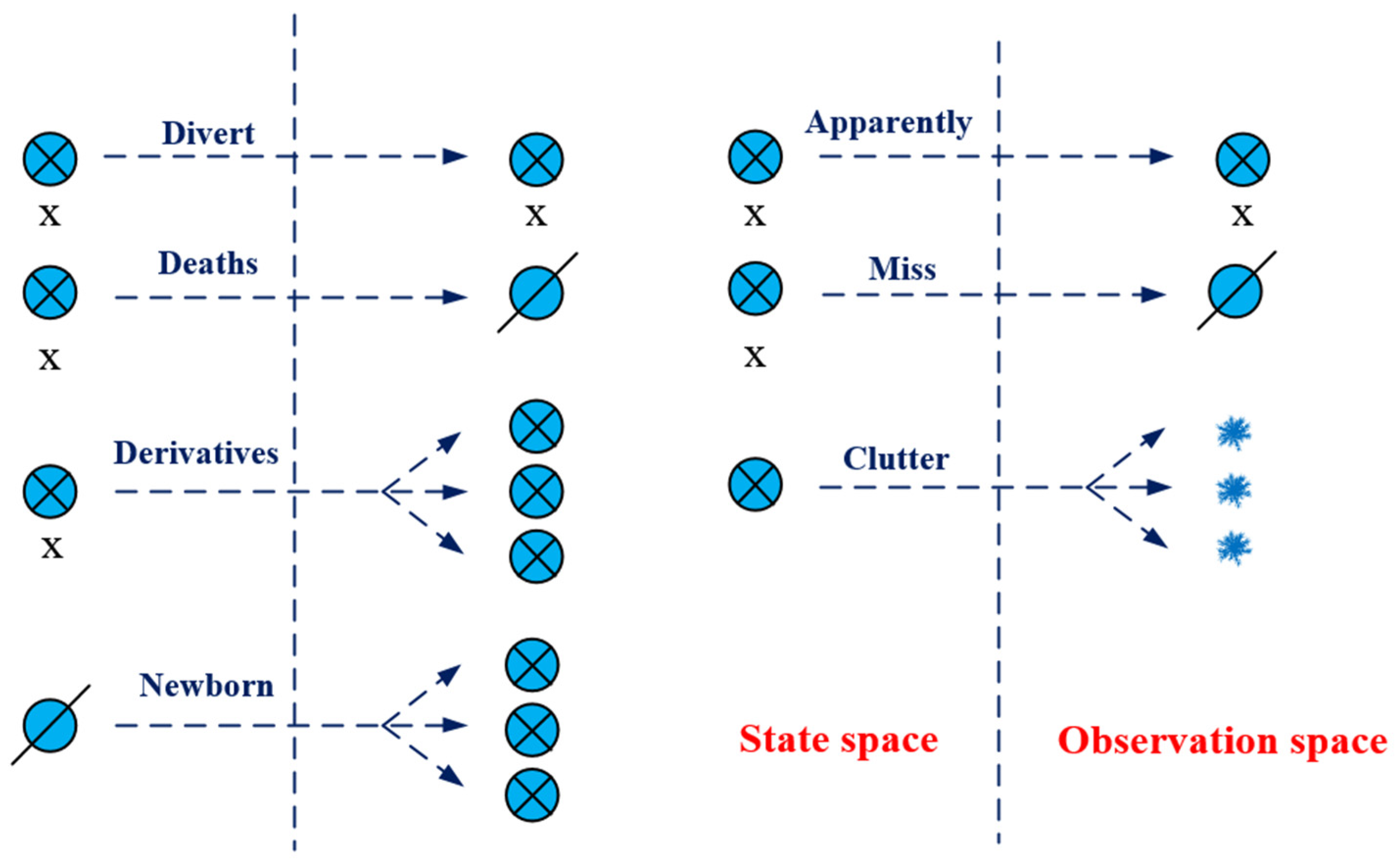
In this study, the GM-PHD filtering algorithm served as the core framework, with the improved spatio-temporal pipeline filtering method integrated into the GM-PHD filtering algorithm to enhance its performance in tracking targets in the space-based observation mode. The GM-PHD filtering algorithm models the multi-target probability hypothesis density using a Gaussian mixture and iteratively updates the individual Gaussian components within the PHD through mean, weight, and covariance initialization, prediction, and update, thereby estimating the target state. As depicted in Figure 1, the GM-PHD method accounts for various scenarios, such as target state transitions, target births, target derivations, and target miss detections, enabling a detailed description of target motion states to achieve multi-target tracking in diverse environments.
The Gaussian mixture form in the GM-PHD algorithm is a linear cumulative representation of multiple weighted Gaussian components used to represent a probability distribution. Each Gaussian component is described by a mean and a covariance matrix. Specifically, the linear cumulative representation of the multi-objective PHD can be expressed as follows:
D k ( x ) = i = 1 J k w k ( i ) N ( x ; m k ( i ) , P k ( i ) )
where D k ( x ) is the probability density function of the multi-objective PHD at state x and time k, J k denotes the number of Gaussian components, m k ( i ) is the Gaussian component mean, w k ( i ) is the Gaussian component weight value, and P k ( i ) is the covariance matrix. The GM-PHD condensed representation takes the following form:
D k = { w k ( i ) , m k ( i ) , p k ( i ) } i = 1 J k
The GM-PHD filtering algorithm for target state estimation consists of five main steps:
  • The probability hypothesis density for multiple targets at the initial moment 0 is
    D 0 ( x ) = i = 1 J 0 w 0 ( i ) N ( x ; m 0 ( i ) , p 0 ( i ) )
The density of multi-target probability assumptions at moment k − 1 is expressed as follows:
D k 1 ( x ) = i = 1 J k 1 w k 1 i N ( x ; m k 1 ( i ) , P k 1 ( i ) )
The expression for the predicted multi-objective PHD is as follows:
D k | k 1 ( x ) = D s , k | k 1 ( x ) + D β , k | k 1 ( x ) + γ k ( x )
where γ k ( x ) is the PHD of the nascent target at moment k , D s , k | k 1 ( x ) is the predicted PHD of the surviving target, and D β , k | k 1 ( x ) is the predicted PHD of the derived target.
The Gaussian mixture of D k | k 1 ( x ) is of the form
D k | k 1 ( x ) = i = 1 J k | k 1 w k | k 1 ( i ) N ( x ; m k | k 1 ( i ) , P k | k 1 ( i ) )
With a given multi-objective PHD D k 1 ( x ) at moment k 1 , the weights, means, and covariance matrices of each of the predicted PHD D k | k 1 ( x ) can be calculated.
The updated multi-objective PHD expression is as follows:
D k ( x ) = ( 1 P D , k ) D k | k 1 ( x ) + z Z k D D , k ( x ; z )
where D k ( x ) is the posterior density, which represents the probability density of the target state at time k after the updating step; P D , k denotes the probability of target detection at time k; D k | k 1 ( x ) is the prior density, which represents the probability density of the predicted state at time k; Z k denotes the set of observations at time k; and D D , k ( x ; z ) denotes the probability density of the target state after updating using the observation data z.
z Z k D D , k ( x ; z ) = z Z k P D , k g k ( z | x ) κ k ( z ) + P D , k g k ( z | ξ ) D k | k 1 ( ξ ) d ξ D k | k 1 ( x )
where P D g k ( z | x ) responds to the probability of observing z in state x. A higher P D , k increases the weight of the observations in the state update, making the algorithm more reliant on the observations for state estimation, and conversely, a lower P D , k decreases the weight of the observations, making the algorithm more reliant on a priori prediction. κ k ( z ) denotes the clutter density function. P D g k ( z | ξ ) D k | k 1 ( ξ ) d ξ denotes the probability density of all possible states at time k corrected by the detection and observation models, which are used to ensure that the probability densities sum to 1. The role of the P D , k is to normalize the probability densities of the observations after updating and to ensure the stability and correctness of the updating process.
g k ( z | x ) = N ( z ; H k x , R k )
where H k is the observation matrix and R k is the observation noise covariance matrix.
The Gaussian mixture of D k ( x ) takes the following form:
D k ( x ) = j = 1 J k | k 1 w k ( j ) ( z ) N ( x ; m k ( j ) ( z ) , P k ( j ) )
At a given time, the updating step computes the mean, weight, and covariance matrix of the updated multi-object PHD using a closed-form solution based on the predicted multi-object PHD at that time and the new observation set.
As the iterations of multi-object PHD prediction and updating progress, the number of Gaussian components continues to increase, resulting in a growing recursive operation for the Gaussian mixture PHD. The number of Gaussian components in the updated PHD D k ( x ) for the Gaussian mixture filter at moment k is as follows:
O ( J k 1 M k ) = ( J k 1 ( 1 + J β , k ) + J γ , k ) ( 1 + M k )
where M k is the number of observations at moment k, J k 1 is the number of Gaussian components of the multi-target PHD D k 1 ( x ) at moment k 1 , and J β , k and J γ , k stand for the number of Gaussian components of the derived and de novo target PHDs at moment k, respectively. This shows that the number of Gaussian components grows uncapped over time.
To ensure the precision of GM-PHD filtering while reducing computational resources, a pruning strategy is employed to address the issue of increasing Gaussian component numbers. Typically, the GM-PHD filter prunes Gaussian components with weights w k ( j ) lower than a predefined threshold, retaining only those with relatively higher weights. Pruning serves to control the number of Gaussian components after each iteration update and reduces the interference of low-weight Gaussian components on state estimation.
In space-based multi-object tracking, the dense concentration of stars can cause multiple Gaussian components to be closely positioned in space, and targets may not be distinguishable from stars. This can lead to the misclassification of stars as targets by traditional GM-PHD filters. Therefore, traditional methods often fail to prune the Gaussian components corresponding to stars, resulting in biased target estimation. To address this issue, this paper proposes a spatio-temporal pipeline filtering method that effectively distinguishes between targets and stars, allowing for the extraction of accurate target information. The specific implementation details will be discussed in Section 3.
After processing through the spatio-temporal pipeline filtering, the resulting pruned and merged multi-object PHD allows for the estimation of the multi-object states from the weight and mean information of the Gaussian components. The estimated number of targets can be determined using Equation (9).
Based on the output of the PHD filter, which is the processed, pruned, and merged multi-target PHD, target states can be estimated from the weight w k ( j ) and mean m k ( j ) ( z ) information of the Gaussian components N ( x ; m k ( j ) ( z ) , P k ( j ) ) . Specifically, for Gaussian components with weights exceeding a predetermined threshold w T H , their means are considered as estimates of the target states. Additionally, for Gaussian components meeting the condition r o u n d ( w k ( j ) ) > 1 , their means m k ( j ) ( z ) are repeatedly counted r o u n d ( w k ( j ) ) times to provide estimation results for the states. Through this step, estimations of the target states and the number of targets can be obtained.
{ m k ( j ) , , m k ( j ) } r o u n d ( w k ( j ) )
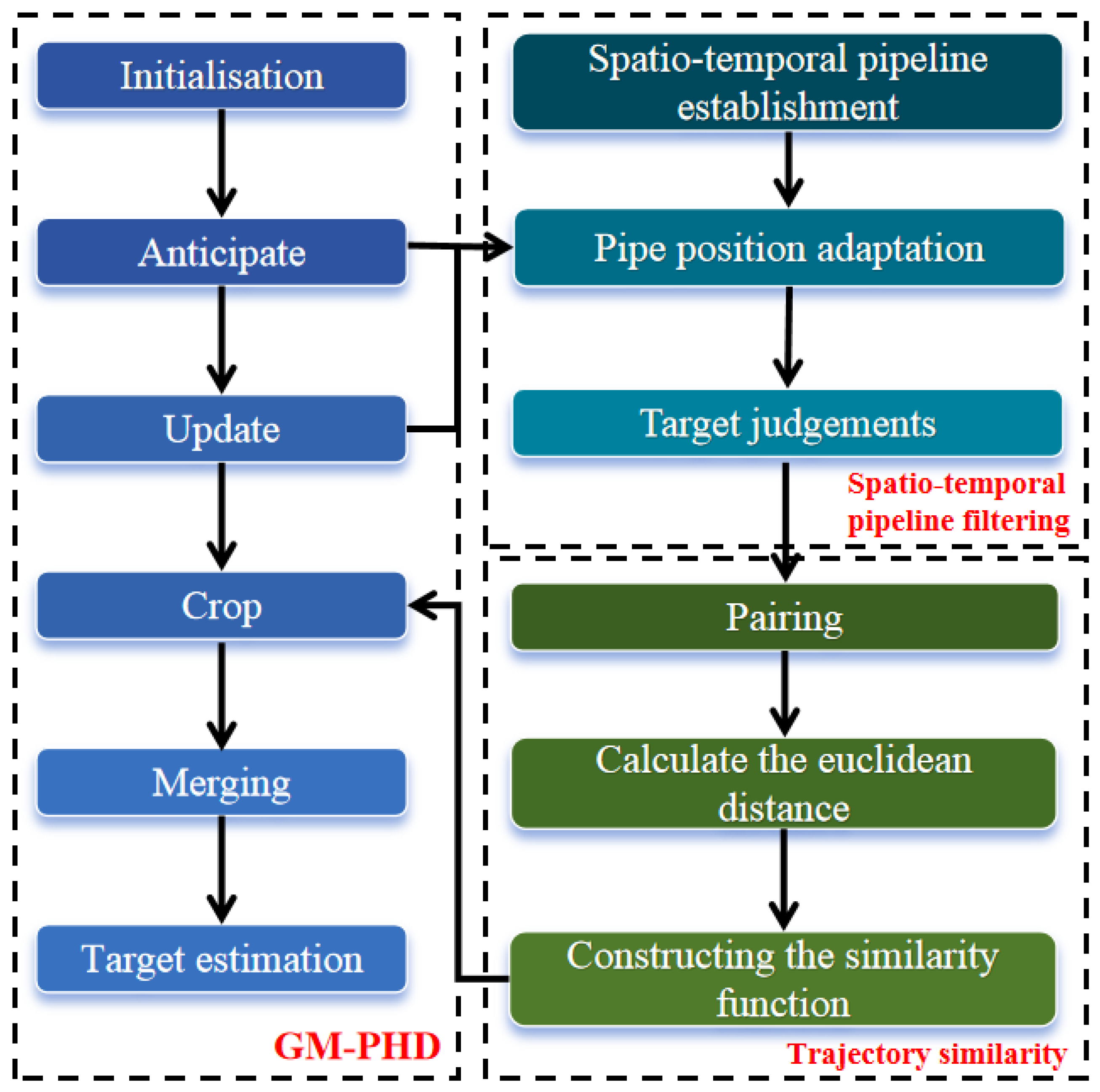
The overall flow of the algorithm proposed in this paper is shown in Figure 2.
As illustrated in Figure 2, the core framework of the multi-target tracking algorithm presented in this paper is based on the GM-PHD filtering method and introduces significant enhancements. The improvements are primarily focused on two aspects:
  • Adaptive spatio-temporal pipeline filtering method: After obtaining the predicted update state of the target using the GM-PHD algorithm, the velocity and position information of the target is determined. This information is utilized to initialize or update the state of the spatio-temporal pipeline filter, thereby capturing the target’s spatial position changes and dynamic information over time. This approach leverages the strengths of both GM-PHD and spatio-temporal pipeline filtering, enabling the algorithm to adapt to dynamic target changes while effectively mitigating noise interference, thus enhancing the continuity and robustness of target tracking.
  • Trajectory similarity method: In star-dense scenes, the traditional GM-PHD filtering algorithm occasionally misjudges stars as real targets due to their weights exceeding the pruning threshold, resulting in tracking deviations. In this study, a trajectory similarity method is employed to distinguish between stars and targets. This method combines the advantages of continuous detection and multi-frame verification inherent in spatio-temporal pipeline filtering. By analyzing the differences in the motion characteristics of targets and stars, stellar weights are pruned effectively, thereby mitigating stellar interference and improving tracking accuracy.

3. Target State Estimation Based on Spatio-Temporal Pipeline Filtering

This paper addresses the problem of target tracking in a space-based environment, particularly in the presence of a large number of stars and noise in the sky background. The traditional GM-PHD algorithm often fails to effectively distinguish targets from background stars when dealing with multiple point targets in the space-based background. To address this issue, this paper proposes a spatio-temporal pipeline filtering method. This method establishes a circular pipeline region around the candidate targets and only considers the pixels within the pipeline when processing the sequence images, instead of processing the entire image as in the traditional GM-PHD algorithm. This approach effectively reduces the interference of background stars and also reduces the computational complexity of the algorithm.
The principle of spatio-temporal pipeline filtering is depicted in Figure 3. The pipeline length comprises L frames of images, and the pipeline window represents a neighborhood centered around the candidate target, which is typically set to be circular. Following the first-in-first-out principle, images entering the pipeline’s top are prioritized for output. The primary rationale for employing this method lies in the clear distributional disparities between targets and noise. A target’s motion trajectory is continuous, and with a judiciously set sampling frame rate and pipeline size, the target’s position in the video sequence image remains relatively stable. Conversely, noise in the video image undergoes random fluctuations and is independent of the target’s trajectory. Hence, the established pipeline enables us to monitor the occurrences of each pixel within the sequence image. Through statistical analysis, points exceeding the predetermined occurrence threshold within the pipeline are identified as candidate targets and retained, while those falling below the threshold are classified as noise and removed accordingly.
The three main parameters of the pipeline filtering algorithm are length, radius, and center position. The pipeline length indicates the number of frames required for detection, which is determined by the range of the target s. If s varies in the interval [0, L], the length of the pipeline is L. The pipeline radius indicates the size of the pixel range containing the target field, which is usually set as a constant. The position of the center of the pipeline is determined by the center coordinates of the spatial target in the current image:
C ( k ) = ( x ( k ) , y ( k ) )
where C ( k ) denotes the center position of the pipe in the kth-frame image target, and x ( k ) and y ( k ) denote the coordinates of the pipe in two dimensions.

3.1. Pipe Position Adaptation

The classical pipeline filtering method typically sets a fixed pipeline radius, denoted as r, which determines the neighborhood range of the target. If the value of r is too small, the pipeline cannot adapt to the target’s motion range, leading to the target appearing outside the pipeline. If r is too large, it results in more noise and interference within the pipeline. Therefore, under the condition of a pipeline radius r, the accuracy of the pipeline center directly determines whether the target can be successfully detected.
In response to the aforementioned issues, this paper proposes improvements to the classical pipeline filtering algorithm. Since the target’s motion trend is continuously smooth, it is possible to combine target state and measurement information to predict the target’s position and velocity, thereby adaptively adjusting the pipeline center and radius. This approach allows better adaptation to the target’s motion range and improves the accuracy of the pipeline center, thereby enhancing the effectiveness of target detection and tracking.
The target state includes the target position as well as target velocity information and obeys a Gaussian linear model:
X ( k ) = [ 1 0 t 0 0 1 0 t 0 0 1 0 0 0 0 1 ] X ( k 1 ) + [ t 2 2 0 0 t 2 2 t 0 0 t ] q k
where X ( k ) = [ x ( k ) , y ( k ) , x ˙ ( k ) , y ˙ ( k ) ] T denotes the state of the target at moment k; [ x ( k ) , y ( k ) ] T and [ x ˙ ( k ) , y ˙ ( k ) ] denote the position and velocity information of the target, respectively; q k denotes the process noise; and t is the sampling period, set to 1 s.
The linear quantitative model is as follows:
Z ( k ) = [ 1 0 0 0 0 1 0 0 ] X ( k ) + ω ( k )
where Z k is the set of target position observations at moment k, and ω ( k ) denotes the measurement noise. The measurement noise is Gaussian white noise, ω ( k ) ~ N ( 0 , σ ω 2 ) , and the variance σ ω = 10   m .
By substituting the target state equation and measurement equation into the prediction and update equations of GM-PHD, the position and velocity of the target can be obtained. Adaptive adjustments to the pipeline center are made based on the predicted target position information. The formula is as follows:
{ C k x = C k 1 x + a x C k y = C k 1 y + a y
where C k x and C k y denote the coordinates of the center of the pipe in the x-axis and y-axis of the kth frame, respectively; C k 1 x and C k 1 y denote the coordinates of the position of the center of the pipe in the k − 1 frame, respectively; and a x and a y denote the error correction terms.
a x = { [ x ( k ) x ^ ( k ) ] 2 + [ x ( k 1 ) x ^ ( k 1 ) ] 2 x ( k ) x ( k 1 ) C k x C k 1 x x ˙ ( k ) t C k x C k 1 x > x ˙ ( k ) t
a y = { [ y ( k ) y ^ ( k ) ] 2 + [ y ( k 1 ) y ^ ( k 1 ) ] 2 y ( k ) y ( k 1 ) C k y C k 1 y y ˙ ( k ) t C k y C k 1 y > y ˙ ( k ) t
where x ^ ( k ) denotes the predicted coordinates of the kth-frame target in the x-axis, and x ^ ( k 1 ) denotes the predicted coordinates of the (k-1)th-frame target in the x-axis. y ^ ( k ) denotes the predicted coordinates of the kth-frame target in the y-axis, and y ^ ( k 1 ) denotes the predicted coordinates of the (k − 1)th-frame target in the y-axis.
To obtain the error correction terms a x and a y in Equations (17) and (18), we follow these steps:
  • We start by determining the target’s velocity and position at moment k using the Gaussian linear model as described by Equation (14), X ( k ) = [ x ( k ) , y ( k ) , x ˙ ( k ) , y ˙ ( k ) ] T .
  • The term m k | k 1 ( i ) , as represented in Equation (6), describes the linear state transition model for the evolution of the target state between moments k 1 and k . The expression is given by
    m k | k 1 ( i ) = F m k 1 ( i ) + B u k 1 ( i )
    where F denotes the state transition matrix, m k 1 ( i ) denotes the target position and velocity values for the ith target at moment k 1 , B denotes the control input matrix, and u k 1 ( i ) denotes the control input. This model provides the predicted values of the target position and velocity at moment k , m k | k 1 ( i ) = [ x ^ ( k ) , y ^ ( k ) , x ˙ ^ ( k ) , y ˙ ^ ( k ) ] .
The value of the error correction terms a x and a y can be obtained from steps 1 and 2. However, the exact values are determined by the difference in the target’s position coordinates between the two frames. The spatio-temporal pipeline filtering center position coordinates C k x , C k 1 x , C k y , and C k 1 y can be obtained from the GM-PHD filter update model described in Equation (10).
The error correction term ensures adaptive adjustment of the pipeline center position. Since the target is in continuous motion, the difference in the target’s center coordinates between two frames is determined by the target’s velocity. Therefore, the error correction term is set as the product of the target velocity, and the sampling period is set as the threshold. If the inter-frame pipeline position difference is less than the error correction threshold, residual compensation is applied to the pipeline center position. If the inter-frame position difference exceeds the error correction threshold, indicating that the position here deviates from the pipeline center due to strong noise interference, the error correction term will remove the current frame position coordinates to avoid pipeline center deviation. Instead, it retains the position coordinates from the previous frame.

3.2. Trajectory Similarity

Although spatio-temporal pipeline filtering methods can effectively distinguish noise from targets, there are challenges when applied to celestial maps due to the presence of a large number of stars. On the one hand, an excessive number of stars on the map leads to the generation of numerous redundant pipelines, thereby wasting computational resources. On the other hand, when multiple stars appear within a pipeline, the algorithm struggles to effectively differentiate between stars and targets. Hence, there is a need to enhance traditional spatio-temporal pipeline filtering methods by incorporating the motion characteristics of celestial objects and background stars, thereby devising an algorithm suitable for celestial systems.
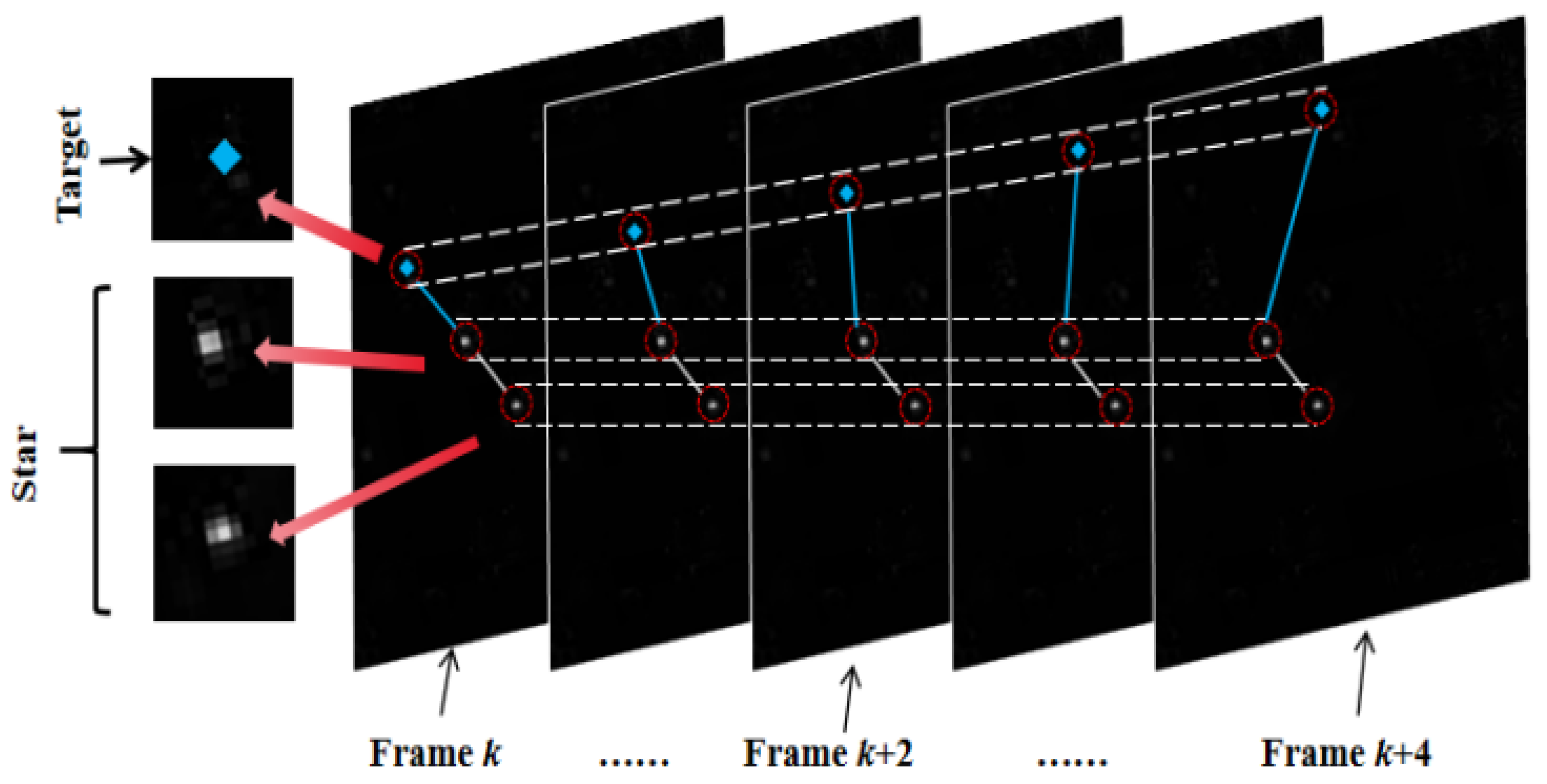
In the star tracking model, as depicted in Figure 4, within each circular pipeline frame, although background stars exhibit random grayscale variations, their overall positional changes across successive frames are not pronounced. Conversely, spatial targets demonstrate distinct motion characteristics, leading to noticeable differences in their positions across frames. Consequently, accurately delineating the characteristic disparities between stars and targets to classify them effectively is pivotal for refining the algorithm.
To address the issue of stellar interference in celestial backgrounds, we employ a trajectory similarity metric [30,31,32] to distinguish between stars and targets. Trajectory similarity refers to the degree of similarity between two or more trajectories in space or time. From Figure 4, it can be observed that as the number of detection frames increases, the distance between stars remains relatively stable, with the white connecting lines between stars hardly changing, indicating strong trajectory similarity. In contrast, due to their motion characteristics, targets exhibit continuous changes in their distances to stars, resulting in the lengths of the blue connecting lines between targets and stars constantly changing. Therefore, we can differentiate between stars and targets based on the differences in their distances. The following describes the steps involved:
  • Pair up the different target points in the sequence of images.
  • For the paired targets, calculate the Euclidean distance between them:
    D n k = ( x n k x n + 1 k ) 2 + ( y n k y n + 1 k ) 2
    where D n k denotes the Euclidean distance of the nth target of the kth frame, and x n k and y n k denote the x-axis and y-axis coordinates of the nth target of the kth frame, respectively.
  • Construct the trajectory similarity function:
    R d = e k = 1 L ( D n k + 1 D n k ) 2 1
    where L denotes the length of the pipeline, D n k + 1 D n k denotes the distance difference between neighboring frames, and the discriminant of the star and target is as follows:
    { 0 < R d < 1 R d 1 R d R Star R d R Target
    where R Star denotes the star trajectory, and R Target denotes the target trajectory. In the star atlas, the center position of the stars changes very little, so the inter-frame distance difference tends to zero. This causes the similarity function R d to vary within the range of (0, 1). In contrast, targets have motion characteristics, so the distance between targets and stars will continue to change, causing the difference in adjacent distances to become larger and larger, resulting in R d values much greater than 1. Based on this characteristic, we can use the value of R d to distinguish between stars and targets in the image and remove the pipeline of R d within the range of (0,1).

4. Experimental Results and Discussion

To ensure the reliability and effectiveness of the simulation experiments, we simulated realistic celestial motion scenarios. The simulation experiments utilized the Tycho-2 star catalog data [33], which include information such as the stellar magnitude, right ascension, and declination. Additionally, Gaussian noise, salt-and-pepper noise, and non-uniform noise were introduced during the imaging process to reflect real-world conditions. In order to demonstrate the algorithm’s versatility, we simulated three scenarios: target crossover, target birth, and targets passing through dense star fields. These scenarios were designed to test the algorithm’s ability to handle complex and dynamic celestial environments. By incorporating these elements into the simulation, we aimed to accurately reflect the challenges of real space surveillance scenarios and assess the algorithm’s performance across a range of conditions.
The simulated star atlas shown in Figure 5 depicts five real target trajectories, each presenting unique challenges. Target trajectory 1 is surrounded by dense stars, testing the algorithm’s capability to track targets amidst significant stellar interference. Trajectory 2 is continuously interfered with by a small number of stars around it, which is used to verify the algorithm’s ability to perform continuous tracking. Trajectories 3 and 4 intersect, challenging the algorithm’s capacity to maintain tracking when targets overlap, and Trajectory 5 belongs to a newborn target, which is used to verify the ability of the algorithm to detect and track a newborn target in the stellar background.

4.1. Ablation Experiments

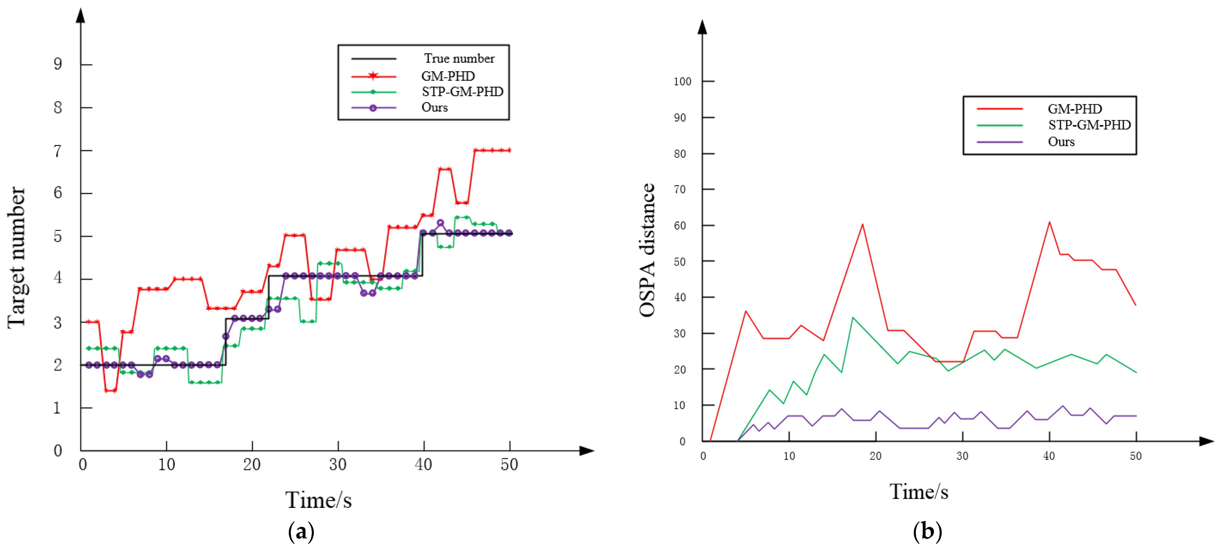
To evaluate the effectiveness of spatio-temporal pipeline filtering and trajectory similarity on the GM-PHD multi-target tracking algorithm, we conducted ablation experiments with three algorithms: GM-PHD, STF-GM-PHD, and the proposed algorithm. GM-PHD serves as the baseline algorithm, STF-GM-PHD combines traditional spatio-temporal pipeline filtering with GM-PHD, and the proposed algorithm incorporates spatio-temporal pipeline filtering and trajectory similarity methods. The linear Gaussian motion model and the observation model of the target are represented by Equations (12) and (13). To balance the detection performance of the sensor and the computational resource consumption of the space-based observation system, this paper sets the detection probability to 95%, and the probability of target survival is 99%. The noise was modeled as Gaussian white noise, and the experimental results are shown in Figure 6.
As shown in Figure 6, in terms of target number estimation, our algorithm most accurately matches the actual number of targets. This demonstrates that the proposed algorithm can better adapt to scenarios with high stellar density. The STP-GM-PHD algorithm, which incorporates spatio-temporal pipeline filtering, shows significant improvement compared with the GM-PHD algorithm. In terms of tracking accuracy, our proposed algorithm achieves the smallest OSPA distance and the best tracking performance. This demonstrates that spatio-temporal pipeline filtering and trajectory similarity are effective in space-based scenarios with high stellar density.
In space-based scenarios, the intensity of the target is typically described in terms of its magnitude; a larger magnitude corresponds to a dimmer brightness [34]. The trajectories in Figure 5 represent targets with five different magnitudes, which are used to further verify the tracking performance of the algorithms in this study for targets with varying intensities. The target magnitudes and signal-to-noise ratios (SNRs) are presented in Table 1.
The formula for calculating the SNR is shown below:
S N R = N s N
where N s denotes the target intensity, and N denotes the noise intensity.
N s = F t × t s × A opt × λ h × c × t 0 × Q s
where F t is the target luminous flux, t s is the exposure time, A opt is the effective pupil area of the sensor, λ is the observed wavelength, h is Planck’s constant, c is the speed of light, t 0 is the transmittance of the optical system, and Q s is the quantum efficiency of the CCD.
N = N s + N B + N D + N R
where N B denotes the background noise, N D denotes the dark current noise, and N R denotes the readout noise.
The SNR is related to the probability of detection as
P D = 1 1 + e a ( S N R b )
where a is the model slope, and b is the threshold value; when the S N R = b , the detection probability is 50%. The results are presented below.
As shown in Figure 7, the detection probability of point targets increases as the SNR increases, and it stabilizes when the SNR reaches 5.
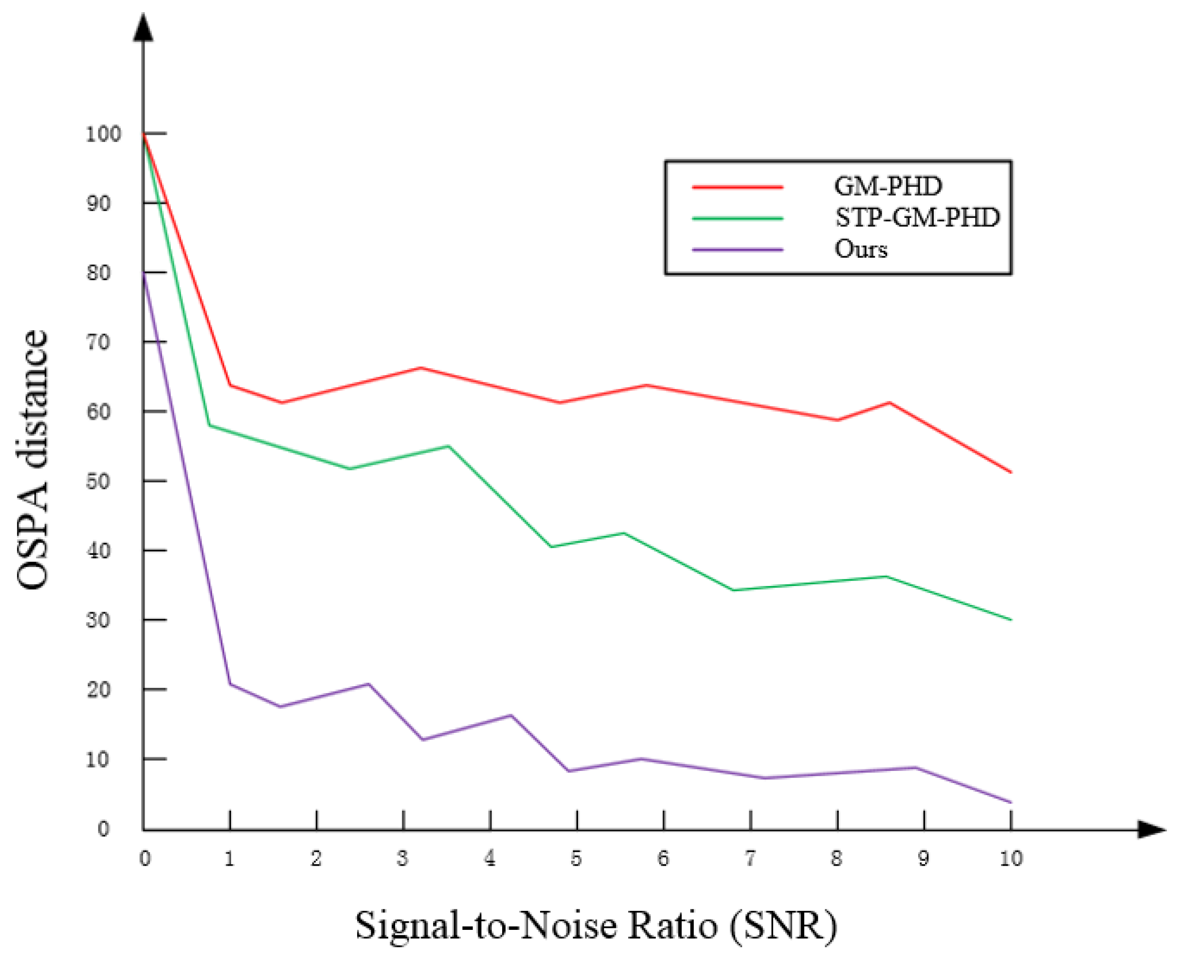
To further verify the relationship between target SNR and tracking performance, OSPA distance analysis experiments were conducted for the three algorithms across a range of SNRs. The results are shown in Figure 8.
Figure 8 shows that the target tracking performance of the three algorithms improves as the SNR increases. However, in comparison, the algorithm proposed in this paper maintains good tracking performance, even when the SNR is 1.
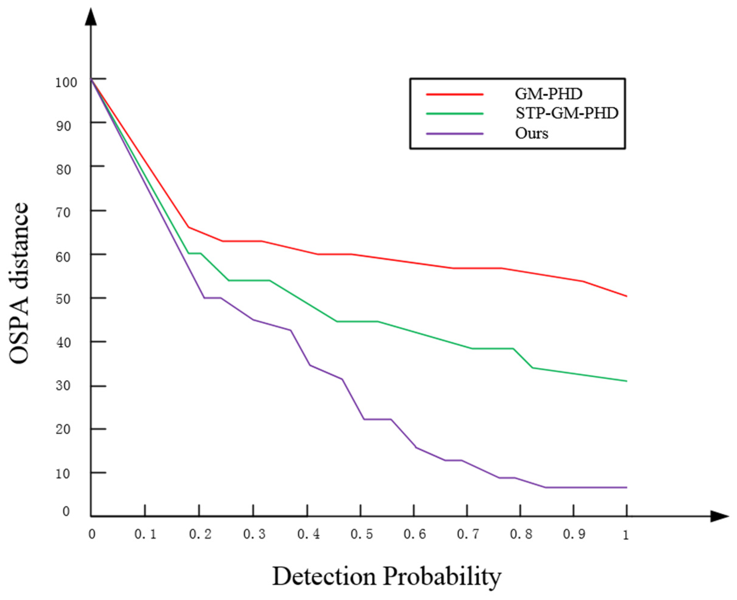
OSPA distance analysis experiments were conducted for the three algorithms under various detection probabilities, with the results presented in Figure 9.
As shown in Figure 9, the OSPA distance for the three algorithms decreases as the detection probability increases. The STP-GM-PHD algorithm outperforms the GM-PHD algorithm, primarily because the introduction of the spatio-temporal pipeline filtering method enables the correlation of multi-frame data and the establishment of a more accurate target state prediction model, which facilitates more precise target state estimation by GM-PHD. The proposed algorithm achieves the lowest OSPA distance, and its OSPA distance error tends to level off when the detection probability is 0.6, remaining between 10 and 20 and converging faster than the other algorithms. This is mainly due to the trajectory similarity method, which effectively differentiates between the target and stars in dense stellar environments, ensuring continuous tracking by the algorithm.

4.2. Simulation Experiment Results

In the simulation data, experiments were conducted to compare the GM-PHD [13], GM-CPHD [35], and SORT [36] with the algorithm proposed in this paper. The experimental parameters were consistent with those used in the ablation experiments, and the results are presented in Figure 10, Figure 11, Figure 12 and Figure 13.
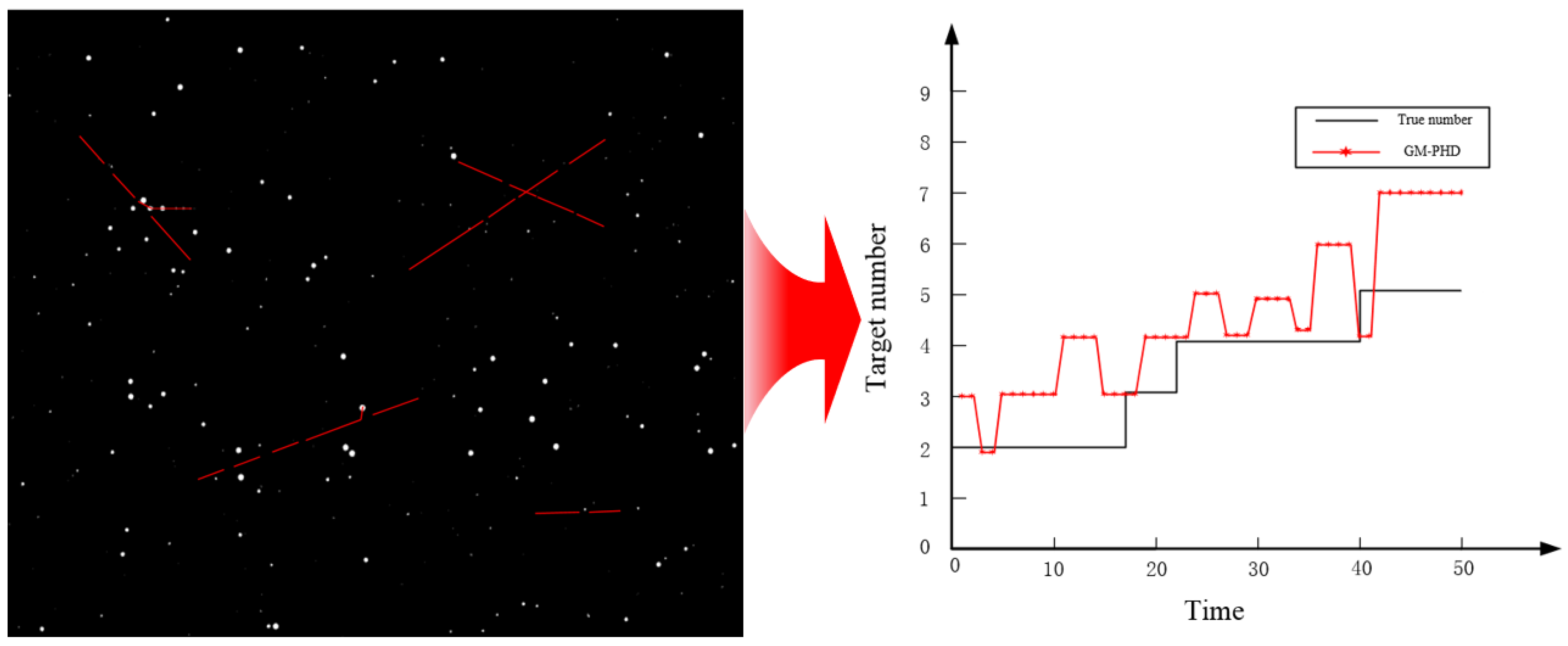
According to the simulation results, GM-PHD, GM-CPHD, and the algorithm proposed in this paper can all effectively track space targets against a stellar background. From Figure 10, it can be observed that although the GM-PHD tracking algorithm can effectively track targets, in the case of dense stars along Trajectory 1, stars may be mistakenly identified as space targets, leading to errors in target number estimation. This is because during the prediction update process, due to the high weight of the stars, the algorithm mistakenly outputs stars as real targets after pruning and merging.
From Figure 11, it can be observed that since the GM-CPHD algorithm introduces the concept of cardinality, it can better handle the uncertainty of target quantity, and compared with the GM-PHD algorithm, it can more accurately estimate the number of targets. However, when dense stars cause overlap between targets and stars, the algorithm struggles to accurately distinguish between different targets, resulting in errors in target number estimation.
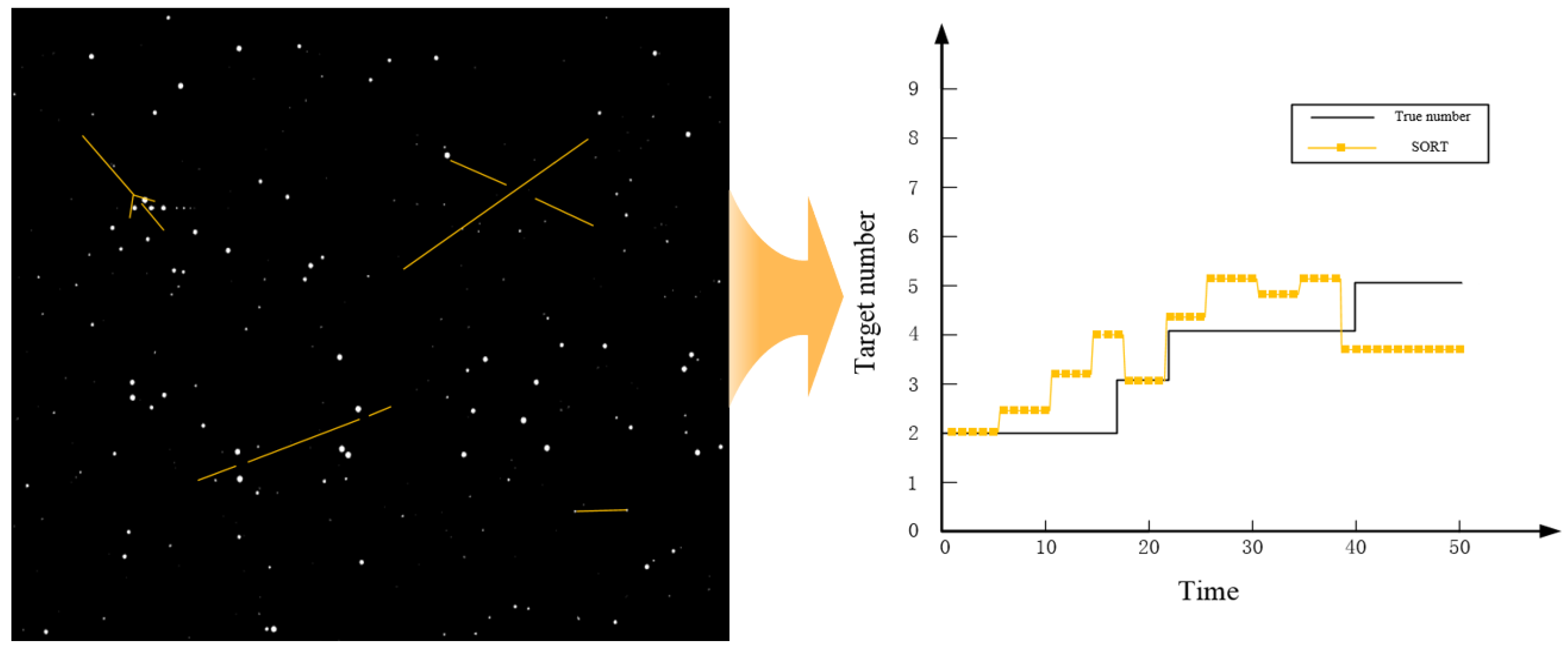
Figure 12 shows that the SORT algorithm can track targets in simple scenarios, but estimation error occurs when stars are dense, targets are newborn, and targets cross. This is because it is difficult for the SORT algorithm to match the detection results with the real targets in space-based complex scenes, which leads to target estimation errors.
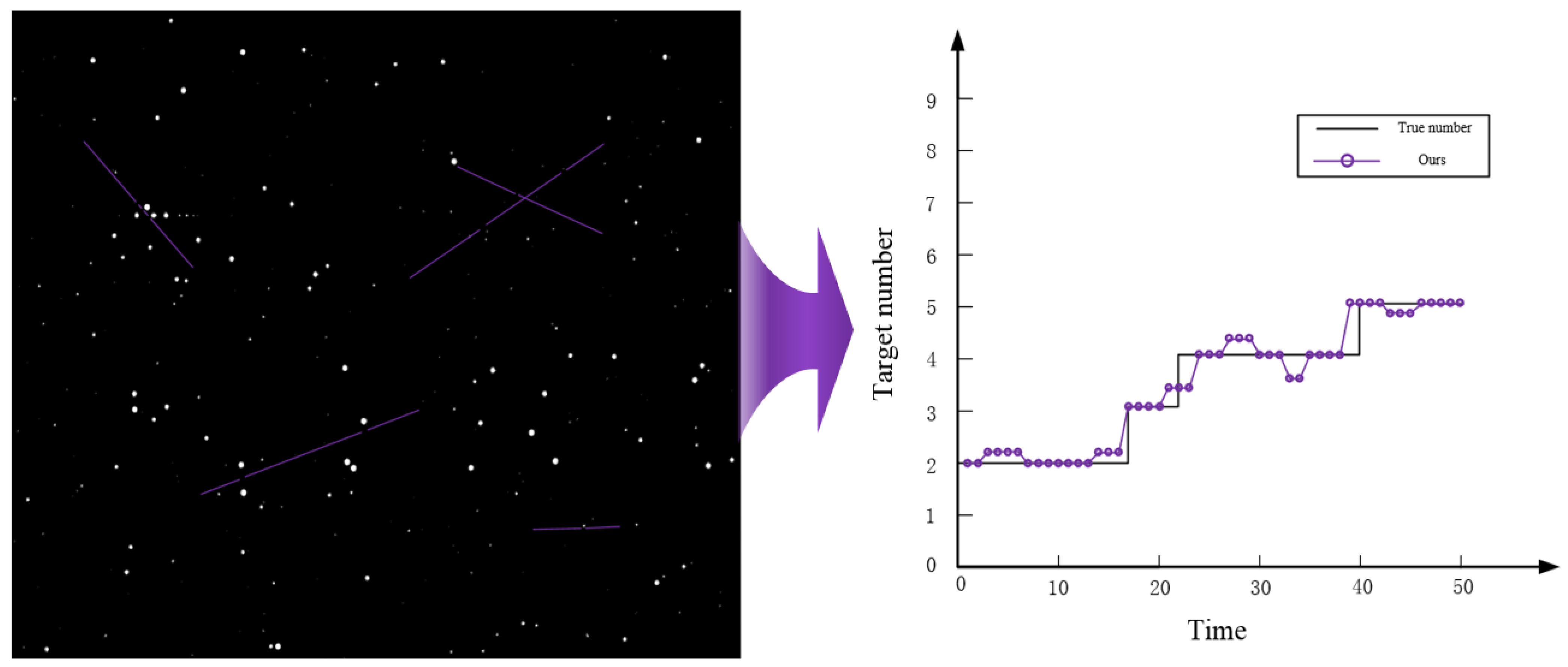
From Figure 13, it can be seen that our algorithm can effectively track targets and estimate target numbers more accurately than the two comparative algorithms. This is because the algorithm in this paper uses a spatio-temporal pipeline to judge the similarity of trajectories between stars and targets, thus avoiding the problem of target misestimation caused by the difficulty of distinguishing between targets and stars.
In summary, the algorithm proposed in this paper performs excellently in target tracking, and its use of the spatio-temporal pipeline method effectively improves the accuracy of target identification and tracking.
When using the GM-PHD algorithm for target tracking and state estimation, it is not only essential to consider the number of targets but also to extract the state information of each target. To evaluate the algorithm’s performance in multi-target state extraction, this paper employs the OSPA (Optimal Sub-Pattern Assignment) distance criterion for further assessment. OSPA takes into account the correspondence between targets and is used to measure the matching degree between two sets of targets. A smaller OSPA distance indicates more accurate estimation results. Its mathematical expression is as follows:
d p ( c ) ( X , Y ) = ( 1 n ( min π n i = 1 m d ( c ) ( x i , y π ( i ) ) p + c p ( n m ) ) ) 1 p
where p denotes the degree of influence of the state bias on the evaluation performance; c denotes the degree of influence of the individual number bias on the evaluation performance, which is usually a truncation constant greater than 0; d ( x , y ) is the Euclidean distance between the elements x and y ; n denotes the set of permutations of { 1 , 2 , , k } ; and π ( i ) denotes the ith number of π in the permutations. X = { x 1 , x m } and Y = { y 1 , y n } are finite subsets, and m and n are positive integers.
Based on the simulation evaluation results in Figure 14, it is evident that within the time interval from 0 s to 50 s, the GM-PHD and SORT algorithms exhibit the largest OSPA distance due to their inability to effectively differentiate between stars and targets, resulting in poor estimation performance. Following this, the GM-CPHD method demonstrates relatively poor estimation results when stars are densely distributed and there are occlusions between targets. As the proposed method in this paper can effectively handle the trajectory relationship between stars and targets, it achieves the shortest OSPA distance and the best tracking estimation performance. Therefore, it can be effectively applied to multi-target tracking scenarios in a space-based context.

4.3. Experiments with Real Star Backgrounds

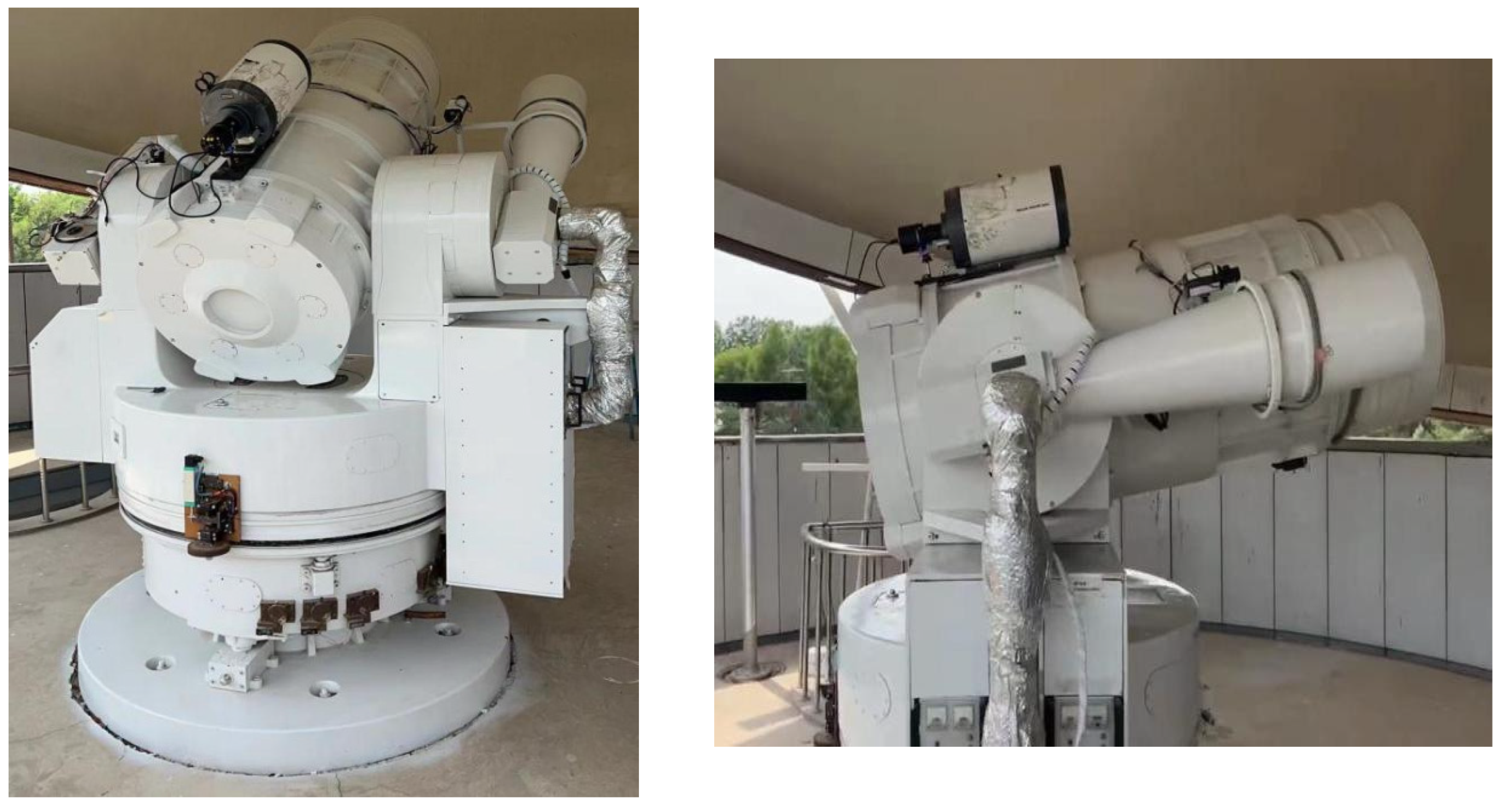
To further validate the algorithm’s tracking capability, we conducted experiments on real stellar background images containing multiple spatial targets. Since there are currently no real-time on-orbit images available from space-based detection systems, we utilized image data captured by ground-based large aperture telescopes, as depicted in Figure 15.
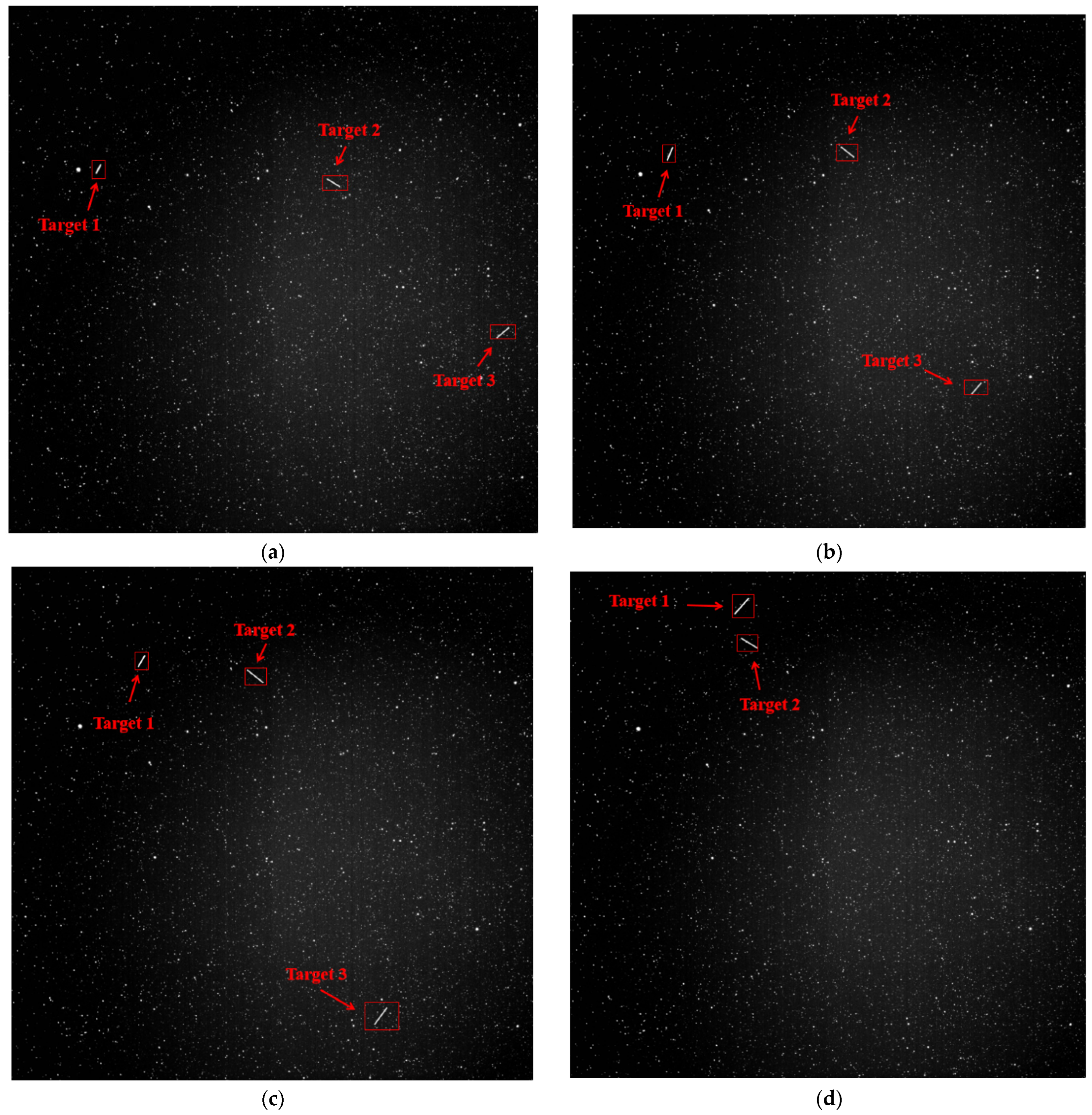
Figure 16 depicts stellar background images captured by ground-based large-aperture telescopes, featuring three trailed targets. These targets exhibit linear motion in the image, with a capture time of 50 s. The image contains some non-uniform noise and salt-and-pepper noise. We extracted frames 5, 15, 35, and 45 from the video. In frame 5, target 1 passes a high-brightness star; in frame 15, target 2 traverses a densely populated stellar region; by frame 30, target 3 is on the verge of disappearing from the star chart; and by frame 45, targets 1 and 2 are nearby, while target 3 has vanished from the star atlas.
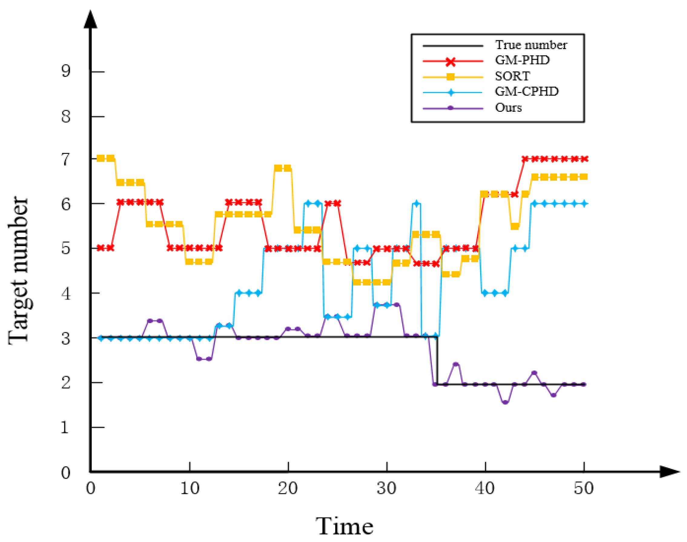
From the actual star atlas tracking results in Figure 17, it can be observed that stars occupy a significant portion of the star atlas with high weights. This causes the GM-PHD filtering algorithm to fail to eliminate high-weight stars during the pruning and merging stages, resulting in misidentification of these stars as targets and ultimately leading to inaccurate estimation of the number of targets. Furthermore, due to the continuous influence of stars, the algorithm’s estimation capability deteriorates over time. In contrast, the GM-CPHD algorithm can better estimate the number of targets compared with GM-PHD, but it suffers from unstable target quantity estimation due to the influence of densely populated stars. The SORT algorithm uses the Hungarian algorithm to solve the data correlation problem, namely that it is difficult to ensure high-precision detection in the presence of stellar occlusion, leading to data correlation errors and thus affecting the estimation of the number of targets. The proposed algorithm in this paper enables accurate target tracking and a more stable and precise estimation of target quantity compared with the two comparison algorithms. It possesses the capability to estimate the number of multiple targets in a space-based scenario.
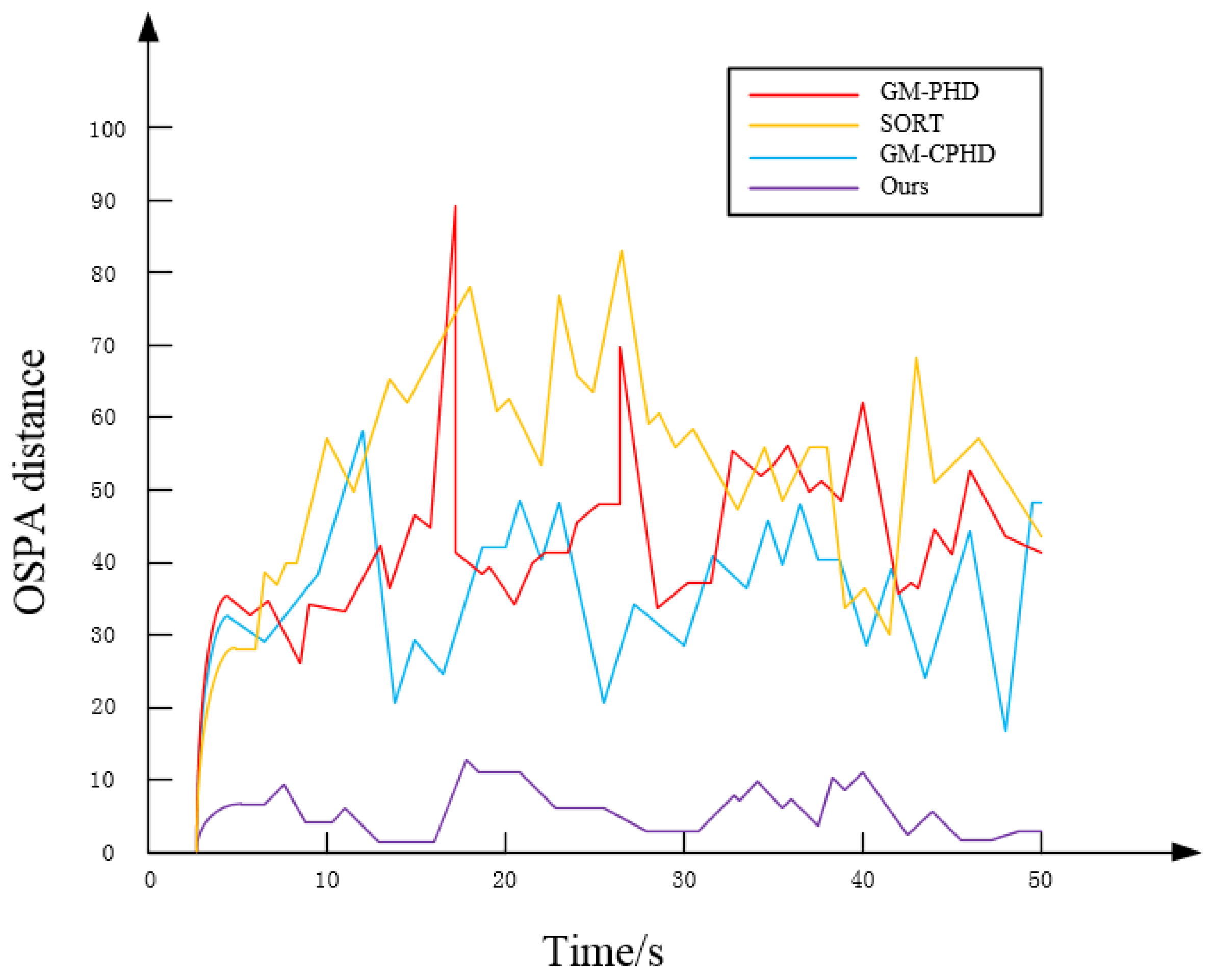
According to the experimental results in Figure 18, it can be seen that the OSPA distance between the GM-PHD and SORT algorithms is larger, because the prediction of the GM-PHD algorithm for the weights of the stars in the tracking process exceeds the pruning threshold, which results in the algorithm misclassifying the stars as the real target. The SORT algorithm uses the Kalman filter to predict the state of the target; in the case of stellar occlusion, this will lead to a reduction in the Kalman filter’s prediction ability, thus affecting the quality of target tracking. Compared with the previous two algorithms, the GM-CPHD algorithm has a smaller overall OSPA distance, indicating higher performance and a better ability to adapt to changes in the number of targets. However, its tracking performance is still affected in regions with dense stellar populations. Compared with the methods mentioned above, the method proposed in this paper performs the best in terms of OSPA distance, indicating its best tracking performance and effective applicability in multi-target tracking scenarios in space-based contexts.

5. Conclusions

This study investigated multi-target tracking algorithms in space-based scenarios. In such contexts, the classical GM-PHD algorithm mistakenly identifies stars passed by targets as actual targets, resulting in errors in target quantity estimation. Therefore, we propose an improved GM-PHD filtering algorithm that effectively removes background noise and stars using spatio-temporal pipeline filtering techniques, which are suitable for space-based multi-target tracking scenarios. Additionally, we improved the spatio-temporal pipeline filtering to adapt to variations in the target velocity and position. We adaptively adjusted the pipeline center position based on the target motion model and incorporated trajectory similarity techniques to more effectively differentiate between the characteristics of stars and targets. We validated the effectiveness of the improved GM-PHD algorithm using both simulated experiments and real experimental data, providing a theoretical basis for multi-target tracking technology in space-based optoelectronic detection systems. In contrast, traditional GM-PHD, GM-CPHD, and SORT algorithms exhibit certain limitations in multi-target tracking in space-based backgrounds. The proposed improved algorithm can better differentiate between stars and targets, demonstrating superior adaptability and tracking performance, and is thus more effectively applicable in space-based multi-target tracking scenarios.

Author Contributions

Conceptualization, Q.F.; Formal analysis, G.W.; Investigation, Y.L.; Software, N.L.; Supervision, H.J.; Validation, L.W.; Visualization, X.W.; Writing—original draft, R.Z. All authors have read and agreed to the published version of the manuscript.

Funding

Funding for this project was received from the Chinese Academy of Engineering (2023-XY-10).

Data Availability Statement

The data presented in this study are available on request from the corresponding author due to confidentiality agreements with our research institution.

Acknowledgments

The authors thank the Project of Chinese Academy of Engineering for helping to identify collaborators for this work.

Conflicts of Interest

The authors declare no conflicts of interest.

References

  1. Fu, Q.; Shi, H.; Wang, C. Research on new technology of photoelectric detection for space-based space debris. Space Debris Res. 2020, 20, 49–55. [Google Scholar]
  2. Esmiller, B.; Jacquelard, C.; Eckel, H.A.; Wnuk, E.; Gouy, Y. Space debris removal by ground-based lasers: Main conclusions of the European project CLEANSPACE. Appl. Opt. 2014, 53, I45–I54. [Google Scholar] [CrossRef] [PubMed]
  3. Zhu, R.; Fu, Q.; Liu, N.; Zhao, F.; Wen, G.; Li, Y.; Jiang, H. Improved target detection method for space-based optoelectronic systems. Sci. Rep. 2024, 14, 1832. [Google Scholar] [CrossRef] [PubMed]
  4. Fu, Q.; Zhao, F.; Zhu, R.; Liu, Z.; Li, Y. Research on the intersection angle measurement and positioning accuracy of a photoelectric theodolite. Front. Phys. 2023, 10, 1121050. [Google Scholar] [CrossRef]
  5. Luo, Q.; Gao, Z.; Xie, C. Improved GM-PHD filter based on threshold separation clusterer for space-based starry-sky background weak point target tracking. Digit. Signal Process. 2020, 103, 102766. [Google Scholar] [CrossRef]
  6. Gong, B.; Jiang, L.; Ning, X.; Li, S. Study on mission planning algorithm for multi-target passive tracking based on satellite formation. Aerosp. Sci. Technol. 2023, 142, 108660. [Google Scholar] [CrossRef]
  7. Liu, E.; Yang, Y.; Yan, Y. Spacecraft attitude tracking for space debris removal using adaptive fuzzy sliding mode control. Aerosp. Sci. Technol. 2020, 107, 106310. [Google Scholar] [CrossRef]
  8. Singh, G.; Kumar, V.; Buduru, A.B.; Biswas, S.K. Tracking an untracked space debris after an inelastic collision using physics informed neural network. Sci. Rep. 2024, 14, 3350. [Google Scholar]
  9. Lin, B.; Wang, J.; Wang, H.; Zhong, L.; Yang, X.; Zhang, X. Small space target detection based on a convolutional neural network and guidance information. Aerospace 2023, 10, 426. [Google Scholar] [CrossRef]
  10. Su, Y.; Chen, X.; Liu, G.; Cang, C.; Rao, P. Implementation of Real-Time Space Target Detection and Tracking Algorithm for Space-Based Surveillance. Remote Sens. 2023, 15, 3156. [Google Scholar] [CrossRef]
  11. Goodman, I.R.; Mahler, R.P.; Nguyen, H.T. Mathematics of Data Fusion; Springer Science & Business Media: Berlin/Heidelberg, Germany, 2013; Volume 37. [Google Scholar]
  12. Mahler, R.P. Multitarget Bayes filtering via first-order multitarget moments. IEEE Trans. Aerosp. Electron. Syst. 2003, 39, 1152–1178. [Google Scholar] [CrossRef]
  13. Vo, B.N.; Ma, W.K. The Gaussian mixture probability hypothesis density filter. IEEE Trans. Signal Process. 2006, 54, 4091–4104. [Google Scholar] [CrossRef]
  14. Vo, B.N.; Singh, S.; Doucet, A. Sequential Monte Carlo methods for multitarget filtering with random finite sets. IEEE Trans. Aerosp. Electron. Syst. 2005, 41, 1224–1245. [Google Scholar]
  15. Fu, Z.; Angelini, F.; Chambers, J.; Naqvi, S.M. Multi-level cooperative fusion of GM-PHD filters for online multiple human tracking. IEEE Trans. Multimed. 2019, 21, 2277–2291. [Google Scholar] [CrossRef]
  16. Zhou, X.; Li, Y.; He, B.; Bai, T. GM-PHD-based multi-target visual tracking using entropy distribution and game theory. IEEE Trans. Ind. Inform. 2013, 10, 1064–1076. [Google Scholar] [CrossRef]
  17. Gonzales, J. An Application of the Finite Set Statistics to Space-Based Multi-Object Tracking. Bachelor’s Thesis, Princeton University, Princeton, NJ, USA, 2023. [Google Scholar]
  18. Wang, X.; Han, C. An improved multiple model GM-PHD filter for maneuvering target tracking. Chin. J. Aeronaut. 2013, 26, 179–185. [Google Scholar] [CrossRef]
  19. Zhang, H.; Ge, H.; Yang, J.; Yuan, Y. A GM-PHD algorithm for multiple target tracking based on false alarm detection with irregular window. Signal Process. 2016, 120, 537–552. [Google Scholar] [CrossRef]
  20. Zheng, S.; Jiang, L.; Yang, Q.; Zhao, Y.; Wang, Z. Adaptive PHD Filter with RCS and Doppler Feature for Space Targets Tracking via Space-Based Radar. IEEE Trans. Aerosp. Electron. Systems. 2023, 1–15. [Google Scholar] [CrossRef]
  21. Jones, B.A.; Gehly, S.; Axelrad, P. Measurement-based birth model for a space object cardinalized probability hypothesis density filter. In Proceedings of the AIAA/AAS Astrodynamics Specialist Conference, San Diego, CA, USA, 1 August 2014; p. 4311. [Google Scholar]
  22. Wang, G. A pipeline algorithm for detection and tracking of pixel-sized target trajectories. In Proceedings of the Signal and Data Processing of Small Targets, Orlando, FL, USA, 1 October 1990; SPIE: Bellingham, WA, USA, 1990; Volume 1305, p. 167. [Google Scholar]
  23. Wang, G.; Inigo, R.M.; McVey, E.S. A single-pixel target detection and tracking system. In Proceedings of the [1990] Proceedings. 10th International Conference on Pattern Recognition, Atlantic City, NJ, USA, 16–21 June 1990; IEEE: New York, NY, USA, 2002; Volume 1, pp. 99–103. [Google Scholar]
  24. Su, Y.; Chen, X.; Cang, C.; Li, F.; Rao, P. A Space Target Detection Method Based on Spatial–Temporal Local Registration in Complicated Backgrounds. Remote Sens. 2024, 16, 669. [Google Scholar] [CrossRef]
  25. Hamida, A.B.; Koubaa, M.; Nicolas, H.; Amar, C.B. Spatio-temporal video filtering for video surveillance applications. In Proceedings of the 2013 IEEE International Conference on Multimedia and Expo Workshops (ICMEW), San Jose, CA, USA, 15–19 July 2013; IEEE: New York, NY, USA, 2013; pp. 1–6. [Google Scholar]
  26. Qian, K.; Zhou, H.; Qin, H.; Yin, S.; Rong, S.; Zhao, D. Infrared Weak Target Tracking Based on Guided Filtering and Spatiotemporal Context. J. Photonics 2015, 9, 151–156. [Google Scholar]
  27. Dong, W.; Zhang, J.; Liu, D.; Wang, X. Pipeline Filtering Algorithm Based on Motion Direction Estimation. J. Photonics 2013, 42, 471–474. [Google Scholar]
  28. Li, J.; Fan, X.; Chen, H.; Li, B.; Min, L.; Xu, Z. Dim and small target detection based on improved spatio-temporal filtering. IEEE Photonics J. 2021, 14, 1–11. [Google Scholar]
  29. Li, Y.; Li, Z.; Zhang, C.; Luo, Z.; Zhu, Y.; Ding, Z.; Qin, T. Infrared maritime dim small target detection based on spatiotemporal cues and directional morphological filtering. Infrared Phys. Technol. 2021, 115, 103657. [Google Scholar] [CrossRef]
  30. Müller, M. Dynamic time warping. In Information Retrieval for Music and Motion; Springer: Berlin/Heidelberg, Germany, 2007; pp. 69–84. [Google Scholar]
  31. Nguyen, T.P.Q.; Phuc, P.N.K.; Yang, C.L.; Sutrisno, H.; Luong, B.H.; Le, T.H.A.; Nguyen, T.T. Time-series anomaly detection using dynamic programming based longest common subsequence on sensor data. Expert Syst. Appl. 2023, 213, 118902. [Google Scholar] [CrossRef]
  32. Wu, X.; Han, J.; Wang, D.; Guo, P.; Cui, Q.; Chen, L.; Liang, Y.; Huang, H.; Lee, H.P.; Miao, C.; et al. Incorporating surprisingly popular algorithm and euclidean distance-based adaptive topology into PSO. Swarm Evol. Comput. 2023, 76, 101222. [Google Scholar] [CrossRef]
  33. Feng, F.; Rui, Y.; Xuan, Y.; Jones, H. Modeling and Calibration of Gaia, Hipparcos, and Tycho-2 astrometric data for the detection of dark companions. Astrophys. J. Suppl. Ser. 2024, 271, 50. [Google Scholar] [CrossRef]
  34. Roberts, S.V. A Space-Based System for Cislunar Space Situational Awareness (Doctoral dissertation, ResearchSpace@ Auckland). Master’s Thesis, The University of Auckland, Auckland, New Zealand, 2024. [Google Scholar]
  35. Svensson, D.; Wintenby, J.; Svensson, L. Performance evaluation of MHT and GM-CPHD in a ground target tracking scenario. In Proceedings of the 2009 12th International Conference on Information Fusion, Seattle, WA, USA, 6–9 July 2009; IEEE: New York, NY, USA, 2009; pp. 300–307. [Google Scholar]
  36. Bewley, A.; Ge, Z.; Ott, L.; Ramos, F.; Upcroft, B. Simple online and realtime tracking. In Proceedings of the 2016 IEEE International Conference on Image Processing (ICIP), Phoenix, AZ, USA, 25–28 September 2016; IEEE: New York, NY, USA, 2016; pp. 3464–3468. [Google Scholar]
Figure 1. Target state and target observation.
Remotesensing 16 02847 g001
Figure 2. Overall framework of the algorithm.
Remotesensing 16 02847 g002
Figure 3. Structure of temporal pipeline filtering.
Remotesensing 16 02847 g003
Figure 4. Framework diagram of spatio-temporal pipeline filtering.
Remotesensing 16 02847 g004
Figure 5. True trajectory of the target.
Remotesensing 16 02847 g005
Figure 6. Comparison of the tracking performance of the three algorithms. (a) Estimated number of star atlas targets. (b) Comparison of OSPA distances.
Remotesensing 16 02847 g006
Figure 7. Detection probability vs. signal-to-noise ratio curve.
Remotesensing 16 02847 g007
Figure 8. OSPA with a range of SNRs.
Remotesensing 16 02847 g008
Figure 9. OSPA at various detection probabilities.
Remotesensing 16 02847 g009
Figure 10. GM-PHD algorithm target estimation results.
Remotesensing 16 02847 g010
Figure 11. GM-CPHD algorithm target estimation results.
Remotesensing 16 02847 g011
Figure 12. SORT algorithm target estimation results.
Remotesensing 16 02847 g012
Figure 13. Our algorithm target estimation results.
Remotesensing 16 02847 g013
Figure 14. Comparison of OSPA distances among the three algorithms.
Remotesensing 16 02847 g014
Figure 15. Ground-based large-aperture telescope.
Remotesensing 16 02847 g015
Figure 16. Actual star charts from a large-aperture telescope. (a) Frame 5. (b) Frame 15. (c) Frame 30. (d) Frame 45.
Remotesensing 16 02847 g016
Figure 17. The estimated number of targets in the star atlas.
Remotesensing 16 02847 g017
Figure 18. Comparison of OSPA distances for a real star atlas.
Remotesensing 16 02847 g018
Table 1. Magnitude and SNR of the targets.
TargetMagnitudeSNR
1114.9674
2108.7275
311.53.6307
4122.5869
5131.2163
Disclaimer/Publisher’s Note: The statements, opinions and data contained in all publications are solely those of the individual author(s) and contributor(s) and not of MDPI and/or the editor(s). MDPI and/or the editor(s) disclaim responsibility for any injury to people or property resulting from any ideas, methods, instructions or products referred to in the content.