Article

Remote Sensing of Chlorophyll-a and Water Quality over Inland Lakes: How to Alleviate Geo-Location Error and Temporal Discrepancy in Model Training

1
Department of Environmental Engineering, Korea National University of Transportation, Chungju 27469, Republic of Korea
2
Department of Food, Agricultural, and Biological Engineering, The Ohio State University, Columbus, OH 43210, USA
3
School of Environment and Natural Resources, The Ohio State University, Columbus, OH 43210, USA
4
Department of Environmental Engineering, Incheon National University, Incheon 22012, Republic of Korea
*
Author to whom correspondence should be addressed.
These authors contributed equally to this work.
Remote Sens. 2024, 16(15), 2761; https://doi.org/10.3390/rs16152761
Submission received: 31 May 2024 / Revised: 20 July 2024 / Accepted: 25 July 2024 / Published: 29 July 2024
(This article belongs to the Special Issue Multi-Source Remote Sensing Data in Hydrology and Water Management)

Abstract

:
Harmful algal blooms (HABs) threaten lake ecosystems and public health. Early HAB detection is possible by monitoring chlorophyll-a (Chl-a) concentration. Ground-based Chl-a data have limited spatial and temporal coverage but can be geo-registered with temporally coincident satellite imagery to calibrate a remote sensing-based predictive model for regional mapping over time. When matching ground and satellite data, positional and temporal discrepancies are unavoidable due particularly to dynamic lake surfaces, thereby biasing the model calibration. This limitation has long been recognized but so far has not been addressed explicitly. To mitigate such effects of data mismatching, we proposed an Akaike Information Criterion (AIC)-like weighted regression algorithm that relies on an error-based heuristic to automatically favor “good” data points and downplay “bad” points. We evaluated the algorithm for estimating Chl-a over inland lakes in Ohio using Harmonized Landsat Sentinel-2. The AIC-like weighted regression estimates showed superior performance with an R2 of 0.91 and an error variance ( σ E 2 ) of 0.29 μg/L, outperforming linear regression (R2 = 0.34, σ E 2 = 2.34 μg/L) and random forest (R2 = 0.82, σ E 2 = 0.92 μg/L). We also noticed the poorest performance occurred in the spring due to low reflectance variation in clear water and low Chl-a concentration. Our weighted regression scheme is adaptive and generically applicable. Future studies may adopt our scheme to tackle other remote sensing estimation problems (e.g., terrestrial applications) for alleviating the adverse effects of geolocation errors and temporal discrepancies.

1. Introduction

Aquatic ecosystems have undergone significant transitions due to climate change, intensifying extreme climate conditions and exacerbating overall water quality [1]. One of the major water quality issues worldwide is the occurrence of harmful algal blooms (HABs), which produce toxins and worsen both aquatic ecosystems and human public health [2]. HABs are classified into various types (e.g., cyanobacteria, dinoflagellates, diatoms, and prymnesiophytes) depending on the relevant organism and the produced toxins [3]. Among these, cyanobacterial HABs are known as major HABs over inland lakes, occurring mainly due to land use/land cover as well as nutrient and sediment loadings [4]. They produce cyanotoxins (e.g., microcystin, cylindrospermopsin, and anatoxins), and in turn threaten aquatic life and human health. To monitor HABs, many researchers have used chlorophyll-a (Chl-a) as a proxy, as it is one of the primary pigments found in all different types of algae. Additionally, many researchers have revealed a strong association between Chl-a and microcystin, major toxins created by cyanobacterial HABs [5,6].
Numerous ground-based networks and sampling campaigns have been carried out across the U.S. to assess water quality conditions. These initiatives have involved government agencies and research institutes, which have utilized buoys and cruises to collect and analyze the physical, chemical, and biological properties of water bodies [7]. However, despite the abundance of in situ measurements across the U.S., two limitations need to be addressed. Firstly, there are constraints on the spatial coverage extent and spatial representativeness of these measurements. The spatial footprint of in situ measurements generally ranges from a few meters to tens of meters depending on the sampling location and instruments used, thus requiring more comprehensive coverage to monitor large-scale water bodies. Secondly, obtaining temporally continuous water quality parameters (WQPs) is challenging due to coarse sampling intervals and adverse weather conditions.
To overcome these limitations, satellite imagery plays a crucial role in monitoring WQPs across various temporal and spatial scales. The fundamental principle of retrieving Chl-a from satellite imagery relies on the spectral signature of the band reflectance (i.e., absorption and reflection), which varies depending on the Chl-a concentration [8]. More specifically, Chl-a tends to reflect green bands and absorb blue and red bands. For the near-infrared range, Chl-a absorbs at 680 nm and reflects at 700 nm. Accordingly, band reflectance from various satellites, including the Landsat series [9,10,11], Sentinel-2/3 [12,13,14,15], and MODerate Resolution Imaging Spectroradiometer (MODIS)/Visible Infrared Imaging Radiometer Suite (VIIRS) [16,17,18,19], has been utilized. For example, Manum et al. [11] developed empirical models to estimate Chl-a over Paldang Reservoir, Korea by using Landsat 5 Thematic Mapper (TM) band reflectance. The results indicated that estimated Chl-a yielded a high coefficient of determination (R2; 0.72), while a relatively high root mean square error (RMSE; 4.9 mg/L) and mean absolute error (MAE; 1.41 mg/L) were observed. Germán et al. [12] utilized Sentinel-2 images (from 2016 to 2019) to quantify spatio-temporal variation in Chl-a in San Roque Reservoir, Argentina by using empirical regression and data mining analysis. Statistical analysis confirmed that the estimated Chl-a showed a high R2 of 0.77. Cao et al. [19] utilized a deep neural network (DNN) to retrieve Chl-a using VIIRS Rayleigh-corrected reflectance over 61 inland lakes located in China. The results indicated that DNN-based Chl-a estimates yielded a relatively low median symmetric accuracy of 28% with an RMSE of 13.8 mg/L. At the same time, however, DNN yielded a high uncertainty in low and high Chl-a concentrations.
An extensive literature review of satellite-based Chl-a retrieval reveals that a general source of uncertainty originates from either geo-registration errors or temporal discrepancies. Geolocation errors are generally caused by spatial mismatch between satellite observations and in situ measurements. The spatial footprint of in situ measurements is a few meters, while the spatial resolution of the optical satellite varies from 30 m (Landsat) to 300 m (Sentinel-3). The evaluation of Chl-a estimates from a sea-viewing wide field-of-view sensor indicated a high uncertainty of Chl-a estimates due to the spatial mismatch between ground- and satellite-based observation [20]. Salama and Su [21] quantified the influence of spatial discrepancy between the Medium Resolution Imaging Spectrometer (MERIS) and field measurement on open-water reflectance. The results indicated that spatial mismatches of 300 and 1000 m cause the uncertainty of reflectance up to 0.02 sr−1 at the red band (665 nm). Accordingly, many researchers have used Landsat-8 and Sentinel-2 with the advantage of relatively high spatial resolution, although temporal mismatch often occurs due to the relatively coarse temporal resolution (Landsat: 16 days, Sentinel-2: 5 days). In addition, the limitations of obtaining satellite-based observation under cloud cover and insufficient sampling activities over an inland lake enhances the temporal discrepancy between satellite- and ground-based measurements.
Here, we aimed to improve remote sensing-based monitoring of water quality by addressing potential geo-registration errors and temporal discrepancies in the matched satellite and ground data. Specifically, we proposed an Akaike Information Criterion (AIC)-like weighted linear regression to estimate Chl-a over inland lakes in Ohio by using HLS band reflectance as an input. The AIC-like weighted linear regression implements an iterative multivariate linear regression (MLR) technique along with a leave-one-out regression process, as well as the Akaike Information Criterion (AIC) for the weighting scheme. For the evaluation, we compared Chl-a estimates from AIC-like weighted regression with those from multivariate linear regression and random forest (RF). Afterward, we additionally analyzed the overall influence of spatial and temporal windows, which have been employed in multiple studies to acquire more matching datasets between ground-based measurements and satellite observations. The rationale behind implementing our proposed method rather than machine learning or deep learning is that it explicitly shows the influence of spatial and temporal windows through the weighting factor to accurately estimate Chl-a.

2. Study Area and Datasets

2.1. Study Area

This study selected inland lakes located within Ohio, with geographical coverage ranging from latitude 38.4°N to 41.98°N and longitude from 80.52°W to 84.82°W (see Figure 1). Ohio’s climate is classified as a humid continental climate according to the Koppen–Geiger classification, characterized by humid and hot summers and cold winters [22,23]. There are relatively large temperature differences between summer and winter, while precipitation shows an even distribution, with 60% of the annual precipitation occurring in the spring and summer seasons [24].
According to the Ohio Environmental Protection Agency (EPA) and Ohio Department of Natural Resources, there are over 50,000 identifiable inland lakes in or partially within the state of Ohio, with 110 natural lakes (with surface area larger than 5 acres) and 113 artificial inland lakes (with surface area larger than 100 acres). Most of the large natural lakes are located in northeastern Ohio, such as Summit, Portage, Stark, and Medina Counties, while artificial lakes are spread throughout the state of Ohio. Among them, some of the major lakes, including the Buckeye Lake and Grand Lake St. Marys (GLSM), suffer from cyanobacterial harmful algal bloom (CyanoHAB) [25,26]. For example, GLSM, one of the largest inland lakes in Ohio, suffered a significant amount of microcystin in July 2010 with the concentration reaching up to 500 μg/L, mainly due to eutrophication originating from agricultural runoff [27].
In addition to the inland lakes in Ohio, a portion of Lake Erie, one of the Laurentian Great Lakes, is included in the study domain. Specifically, this study focuses on the western basin of Lake Erie, which extends from the city of Toledo to Sandusky. The Western Lake Erie region consistently suffers from cyanobacterial HAB due to nutrient loadings from agricultural runoff from the Maumee River watershed [28,29]. This has led local governments to spend about $3 million per year to address the cyanotoxins in drinking water [30,31].

2.2. Datasets

2.2.1. Ground-Based Chlorophyll-a Measurements

This study collected ground-based chlorophyll-a (Chl-a) observations via fluorometer from various sources, including the following: (1) National Water Information System (NWIS) from the United States Geophysical Survey (USGS), (2) Sustaining the Earth’s Watersheds, Agricultural Research Data System (STEWARDS) from the United States Department of Agriculture (USDA) Agricultural Research Services (ARS), (3) STOrage and RETrieval Water Quality (STORET) from the United States Environmental Protection Agency (EPA), (4) AquaSat [32], (5) Ohio Sea Grant and Stone Laboratory, and (6) Great Lake Environmental Research Laboratory (GLERL) of the National Oceanic and Atmospheric Administration (NOAA). Among these sources, Chl-a measurements from NWIS, STEWARDS, and STORET over inland lakes in Ohio were accessible from the National Water Quality Council (https://waterqualitydata.us, accessed on 28 May 2022).
Ohio Sea Grant and Stone Laboratory have been collecting water quality samples via charter boat captains and science cruises since 2013 to efficiently monitor water quality and algal blooms in Lake Erie [33]. They use a surface-to-2-m intergraded tube sampler to obtain various water quality parameters (WQPs), including chlorophyll, microcystin, and Secchi depth, along with ancillary information (e.g., water depth, water temperature, and geographic location). The dataset can be obtained through the Stone Lab Algal and Water Quality Laboratory (https://ohioseagrant.osu.edu/research/live/water, accessed on 7 April 2022).
NOAA GLERL has also initiated the HAB monitoring field campaign over the western part of Lake Erie since 2012 [34]. NOAA GLERL provides biological, chemical, and physical properties of water quality through weekly sampling (from May to October), as well as seven buoys deployed over the western part of Lake Erie that provide temporally continuous observations. Note that sampling density may vary at each station due to environmental conditions such as weather constraints [35]. The NOAA GLERL dataset can be obtained from the NOAA-GLERL website (https://www.glerl.noaa.gov/data/#biological, accessed on 10 May 2022).

2.2.2. Harmonized Landsat and Sentinel-2 (HLS)

Harmonized Landsat and Sentinel-2 is a project initiated by the National Aeronautics and Space Administration to combine the surface reflectances from Landsat 8 Operational Land Imager (OLI) and Sentinel-2 Multi-spectral Instrument (MSI) [36]. The original surface reflectances from Sentinel-2 MSI and Landsat-8 OLI have slight differences in revisit frequency (MSI: ~5 days near equator; OLI: 16 days), spectral resolution, and spatial resolution (MSI: 10–60 m; OLI: 30 m [visible, near, and shortwave infrared] and 100 m [thermal]). Accordingly, the HLS datasets underwent several processing steps to harmonize the two datasets. First, atmospheric correction (Landsat Surface Reflectance Code) and cloud mask were applied to both Landsat-8 and Sentinel-2 imagery. Then, a geometric co-registration and resampling, bi-directional reflectance distribution function was applied to normalize based on viewing and illumination angles. Then, the bandpass of Sentinel-2 was adjusted based on the Landsat-8 bandpass, which was based on the algorithm developed based on the Hyperion sensor [37]. After the harmonization process, the HLS datasets provided the global surface reflectance every 2–3 days with a spatial resolution of 30 m on the Universal Transverse Mercator (UTM) projection. The temporal coverage of the HLS was April 2013 and October 2015 for Landsat 8 and Sentinel-2, respectively. The evaluation of surface reflectance from HLS by comparing against the Moderate Resolution Imaging Spectroradiometer (MODIS) product revealed good consistency between the two, with a relative uncertainty of less than 11% [36]. Considering the spectral signature of Chl-a, as well as the overlapping spectral bands of Landsat-8 and Sentinel-2, this study implemented eight spectral bands (Table 1) from April 2013 to December 2021 to estimate the chlorophyll-a over inland lakes in Ohio.

3. Methodology

3.1. Data Processing and Quality Control

One of the major challenges encountered in water quality monitoring via satellite-based observation is acquiring enough matched datasets between ground- and satellite-based measurements. For instance, the lack of ground-based water quality datasets, along with the relatively coarse temporal resolution of optical imagery, reduces the number of available datasets for the estimation. In addition, if locally developed clouds contaminate only a small portion of the study domain, we can acquire more datasets by obtaining surface reflectance from nearby pixels. Accordingly, two aspects are generally considered: (1) spatial window and (2) temporal window. The major assumption in using various spatio-temporal windows is that water quality conditions remain relatively homogeneous over the extended spatio-temporal windows if there are no significant climate conditions causing any types of mixing [38]. Accordingly, many researchers have explored to find optimized spatial [39,40,41] and temporal windows [37,42,43], but a consensus has not been reached. Thus, this study utilized a spatial window of up to 8 neighboring pixels (~500 m) and a temporal window of ±5 days to collect satellite observations and further analyze the influence of different spatio-temporal windows.
Before conducting the AIC-like weighted linear regression to estimate Chl-a, all datasets collected from different sources underwent quality control (QC) processes. Firstly, we only considered ground-based measurements collected near the water surface, as more than 90% of the reflected signals from a water body originate from the water surface [44]. Additionally, ground-based measurements located within 30 m of the shoreline were discarded to avoid the inclusion of bottom reflectance in shallow waters along the shoreline. Furthermore, negative values and outliers from ground-based Chl-a (e.g., those outside the range of three standard deviations) were not considered. Finally, if specific pixels from either Sentinel-2 or Landsat 8 were cloud-contaminated (indicated by QC flags from HLS), the corresponding ground-based measurements were discarded to minimize the uncertainty triggered by clouds. As a result, only 42% of the datasets were available for model development and validation. Accordingly, we divided them into 6:4 for model development and validation.

3.2. Akaike Information Criterion (AIC)-like Weighted Regression

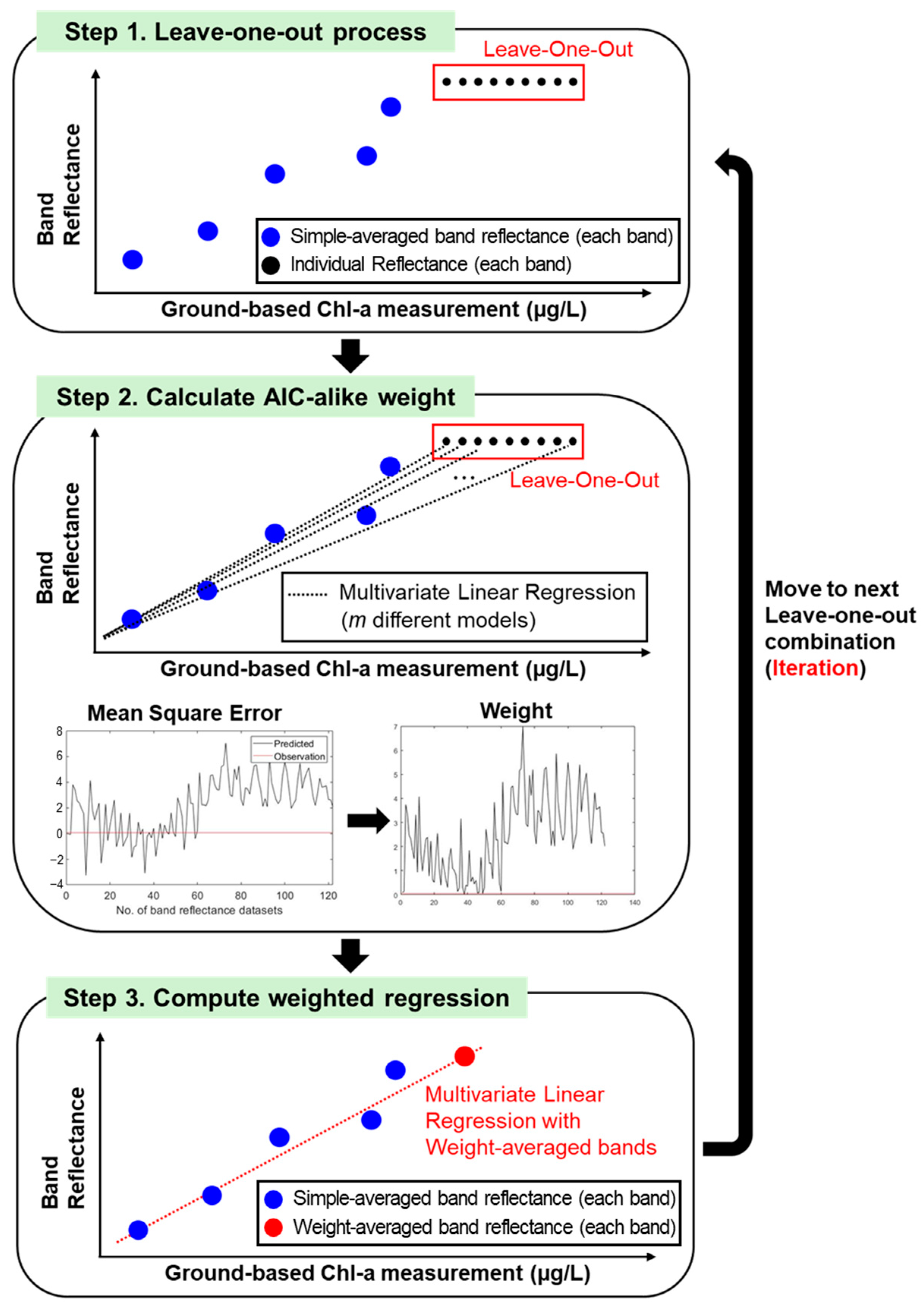
In order to analyze the influence of geo-registration error and temporal discrepancy in model training, this study proposed AIC-like weighted regression. The overall framework is summarized in Figure 2. The proposed algorithm consists of three main parts: (1) conduct a leave-one-out process, (2) calculate AIC-like weight, and (3) compute weighted linear regression.
Suppose we have n combinations of surface reflectance (for each band) from HLS paired with n ground-based Chl-a measurements across the study domain during the study period. Note that each surface reflectance combination comprises multiple surface reflectance observations (8 different band spectra for each observation) depending on different spatio-temporal windows (described in Section 3.1). The first step is to select one pair of surface reflectance combinations (composed of 8 bands) and the corresponding Chl-a measurement. The underlying motivation for leave-one-out weighted linear regression framework originated from leave-one-out cross-validation. This technique has been widely applied to evaluate the statistical performance of both classification and regression algorithms [45]. Although leave-one-out cross-validation is computationally intensive as it requires repetition, it can minimize the error magnitude by utilizing as many datasets as possible to build the statistical model.
Then, the remaining n-1 combinations of surface reflectance for each band will be averaged, and in turn, we obtain n-1 combinations of simple-averaged surface reflectance for each band and the corresponding Chl-a measurement, which will be used as predictor and independent variables, respectively. For the leftover combination of surface reflectance, we also use m individual band reflectance from each band (before averaging) and the corresponding ground-based Chl-a measurement. This allows us to develop m different multivariate linear regression models and calculate the mean square error (MSE) based on different regression models. Subsequently, AIC-like weight is calculated by considering the MSE of different regression models following Equation (1):
w ( i ) = 1 ( y i ^ y ) 2 i = 1 m 1 ( y i ^ y ) 2
where y i ^ denotes the estimated Chl-a from mth regression model and y represents the ground-based Chl-a measurement. m represents the different number of surface reflectance observations within the nth combination. The underlying concept of Equation (1) comes from AIC in that assigning more reliability toward the model yields a smaller magnitude of MSE. More specifically, Equation (1) indicates the greater weight will be assigned to surface band reflectance, which provides Chl-a estimates that closely match the ground-based Chl-a measurement. Once the weight calculation is completed, it is further compared with the Chl-a estimates based on using simple average of the surface reflectance to ensure that weighted average of the surface reflectance will provide more accurate Chl-a estimates. If not, weighted average of the surface reflectance will be replaced with the simple averaged value. Afterward, we move to the next pair of surface reflectance combinations and ground-based measurement and repeat the same procedure.

3.3. Evaluation Metrics

To evaluate Chl-a estimates from HLS and AIC-like weighted linear regression, we calculated Chl-a estimates from both multivariate linear regression (MLR) and RF. MLR-based Chl-a estimates were calculated by using HLS surface reflectance of same-day observations (temporal windows of 24 h) at specific pixel-containing measurement locations. The same matched-up datasets were used to calculate the RF-based Chl-a estimates with additional hyperparameter optimization scheme (gridsearchCV).
For quantitative evaluation, statistical metrics including the coefficient of determination (R2), bias, mean absolute error (MAE), error variance ( σ E 2 ) , and root mean square error (RMSE) were computed using the following equations:
R 2 = N j = 1 N ( y j ^ × y j ) j = 1 N ( y j ^ ) j = 1 N ( y j )   [ N j = 1 N ( y j 2 ^ ) ( j = 1 N ( y j ^ ) ) 2 ] [ N j = 1 N ( y j ) ( j = 1 N ( y j ) ) 2 ]
b i a s = 1 N i = 1 N ( y j ^ y j )
M A E = 1 N j = 1 N | y j ^ y j | ,
R M S E = 1 N j = 1 N ( y j ^ y j ) 2
where N represents the total number of ground-based Chl-a measurements over the study period across the inland lakes in Ohio; y j ^ and y i denote the jth estimated and measured Chl-a value, respectively. Note that σ E 2 is calculated as the square of the RMSE.

4. Results and Discussion

4.1. Overview of Chlorophyll-a over Inland Lakes in Ohio

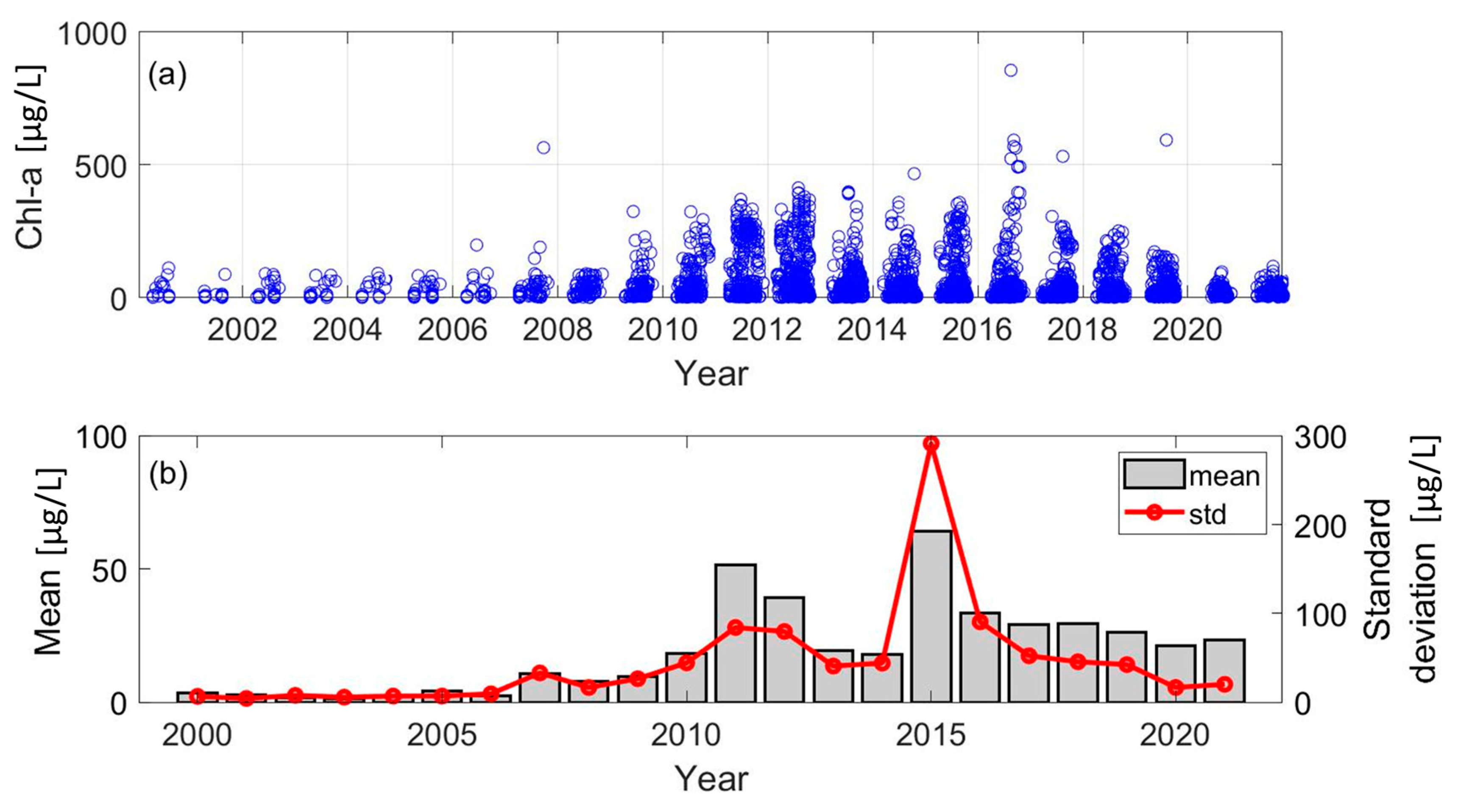
Before evaluating Chl-a estimated using surface reflectance from HLS and AIC-like weighted regression, we analyzed the overall temporal behavior of Chl-a measured through sampling activities across inland lakes in Ohio from 2000 to 2020. The results indicated that the overall concentration of Chl-a (Figure 3a) increased from 2000 to 2013, although the mean concentration of Chl-a slightly decreased from 2011 to 2013 (Figure 3b). Afterward, the mean concentration of Chl-a showed a significant increase in 2015, with the largest standard deviation of 291.49 µg/L, followed by a slight decrease. The maximum Chl-a concentration during the study period was 856 µg/L at Buckeye Lake during the year of 2016, indicating a high eutrophication level.
Focusing on the top five annual maximum Chl-a concentrations since 2010, they were generally observed at Grand Lake St. Marys (GLSM), Buckeye Lake, and Lake Erie, which was also witnessed by Gorham et al. [25] More specifically, 99.2% of the observed Chl-a concentrations (i.e., 514 out of 519) at Buckeye Lake and GLSM yielded Chl-a concentrations of over 56 µg/L, suggesting hypereutrophic conditions [46]. Both GLSM and Buckeye Lake have similar causes for high Chl-a concertation: non-point source pollutant loading. For example, GLSM is affected by pollutants from non-irrigated crop production, residential development, and livestock feeding operations [47]. In the case of Buckeye Lake, it routinely suffered algae blooms every year after 2010 due to nearby crop fields, accounting for 40.6% of the land cover in Buckeye Lake [48]. The Buckeye Lake reservoir experienced a high Chl-a concentration during 2015–2016 with the mean Chl-a concentration of 248.59 µg/L, which corresponds to the algae warning issued by the Ohio Department of Natural Resources.
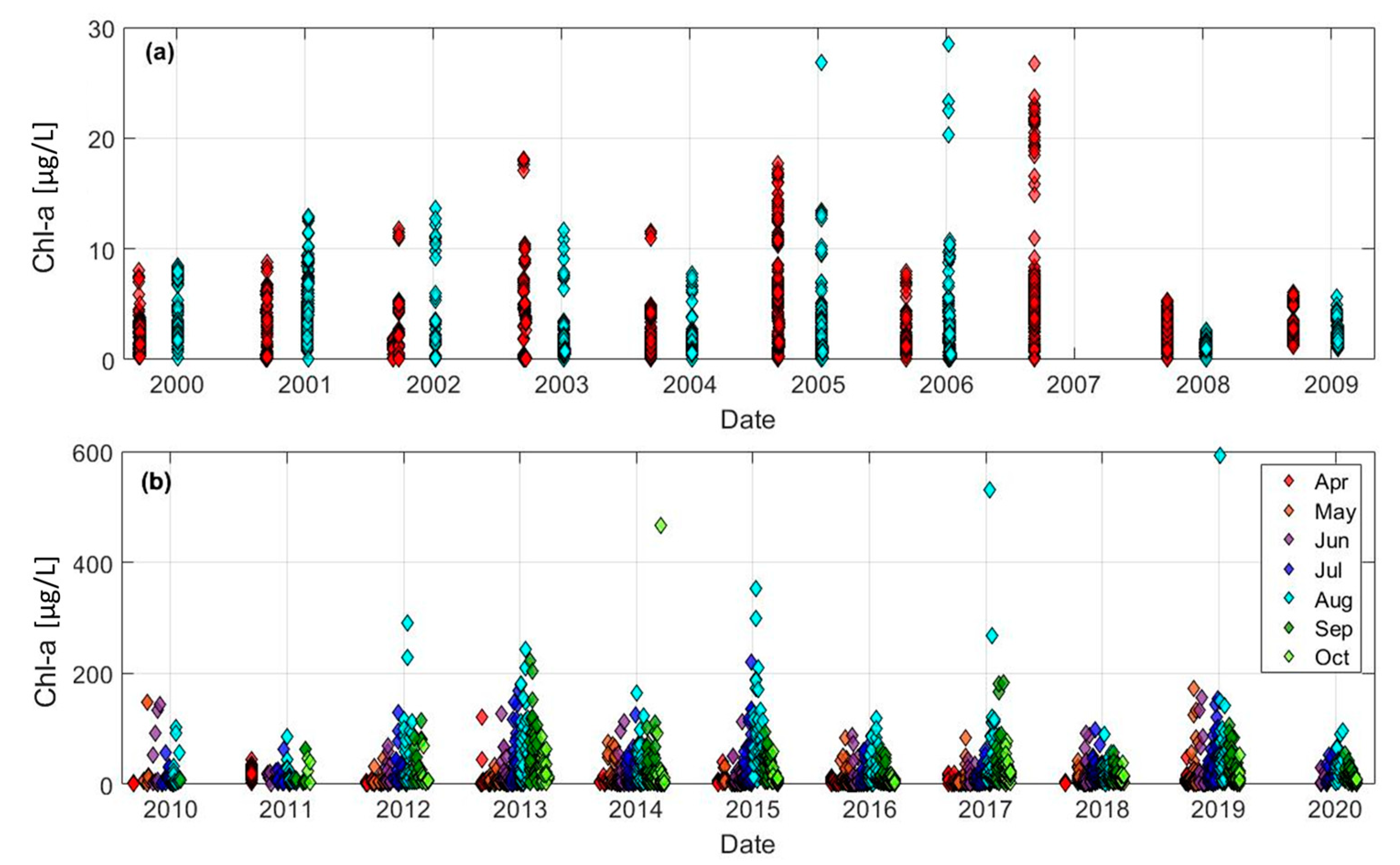
Figure 4 depicts the time series of Chl-a samples collected across Lake Erie during the study period. Note that the period from 2000 to 2009 is illustrated separately, as the EPA Great Lakes National Program sampled water quality parameters only during April and August of each year. The main difference between the periods before and after 2010 is the magnitude of the Chl-a concentration. The overall mean Chl-a concentration before 2010 was 2.20 µg/L, with annual averages ranging from 0.74 µg/L to 5.50 µg/L. In contrast, the later period yielded a mean Chl-a concentration of 13.55 µg/L, with the maximum annual average Chl-a of 31.49 µg/L occurring in 2015. According to Figure 4b, Chl-a measurement exceeding 200 µg/L was first observed in August 2011, corresponding to the substantial algal bloom that occurred in Lake Erie from June to October 2011. Michalak et al. [49] reported that the peak bloom intensity in August 2011 was 7.3 times higher than that from 2001 to 2009, caused by phosphorus loading from agricultural practices coupled with meteorological conditions such as heavy rainfall and discharge.
In terms of seasonal behavior, the maximum Chl-a concentration was generally measured in August of each year after 2010 (Figure 4b). This pattern aligns with the positive relationship between lake surface temperature and Chl-a concentration. Kraemer et al. [50] noted that phytoplankton incubate more readily under warming conditions, leading to an increase in phytoplankton biomass in lakes due to enhanced energy transfer to phytoplankton consumers. Additionally, changes in meteorological conditions and land cover triggered by warming can increase nutrient inflow into the lake. In 2014, the maximum Chl-a concentration was observed in October, corresponding to a harmful and nuisance cyanobacterial algal bloom in Lake Erie. This bloom further overwhelmed the water treatment system in the city of Toledo [51].

4.2. Evaluation of Chlorophyll-a Estiamtes from AIC-like Weighted Regression

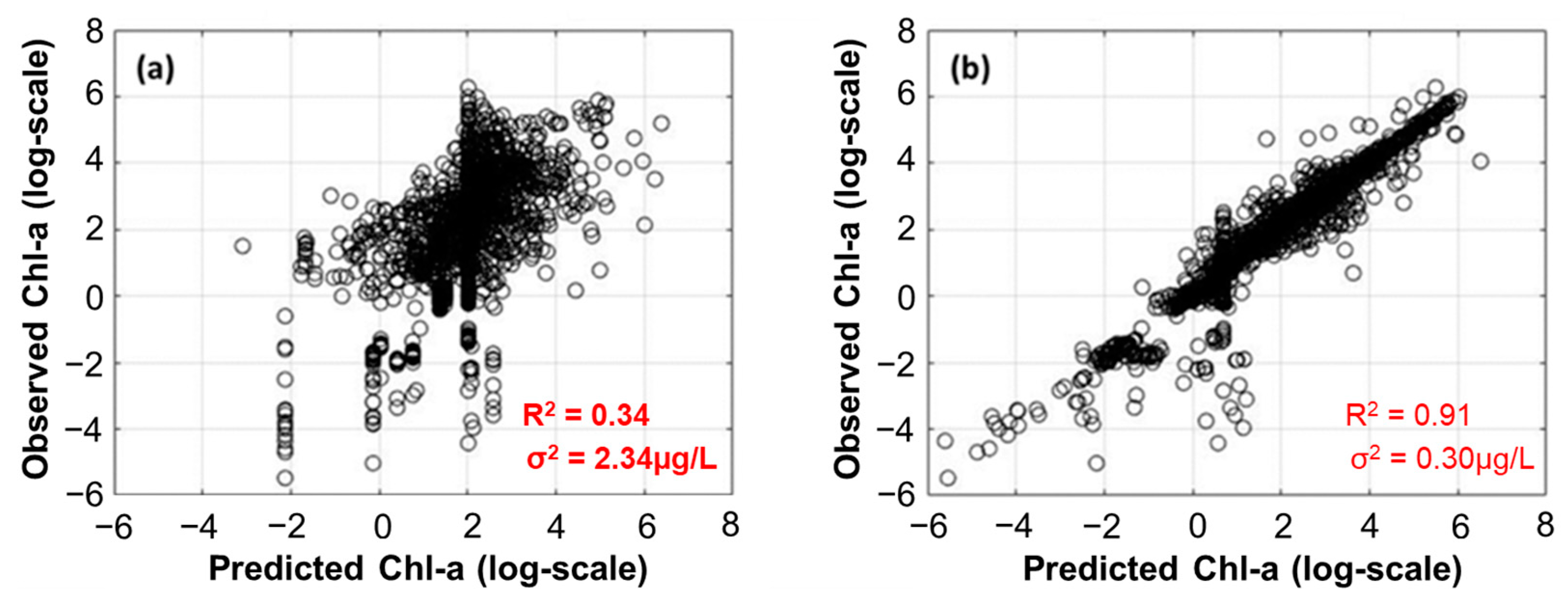
To examine the statistical performance of AIC-like weighted regression, we compared the Chl-a estimates from both multivariate linear regression and AIC-like weighted regression against Chl-a observed from the ground-based stations (Figure 5). Overall, the results indicated that AIC-like weighted regression yielded better consistency with ground-based measurements. Specifically, the coefficient of determination (R2) of the AIC-like weighted regression was 0.91, which was significantly higher than the R2 of multivariate linear regression (0.34). Similarly, the error variance of estimated Chl-a from AIC-like weighted regression (0.30 µg/L on a log scale) was also an improvement over that of multivariate linear regression (2.34 µg/L on a log scale). Additionally, Chl-a estimates from AIC-like weighted regression showed better statistics than those estimated from a random forest model with an R2 of 0.82 and an error variance of 0.92 µg/L. While the random forest model performed better than multivariate linear regression, the AIC-like weighted regression proposed in this research demonstrated the best agreement with ground-based observations.
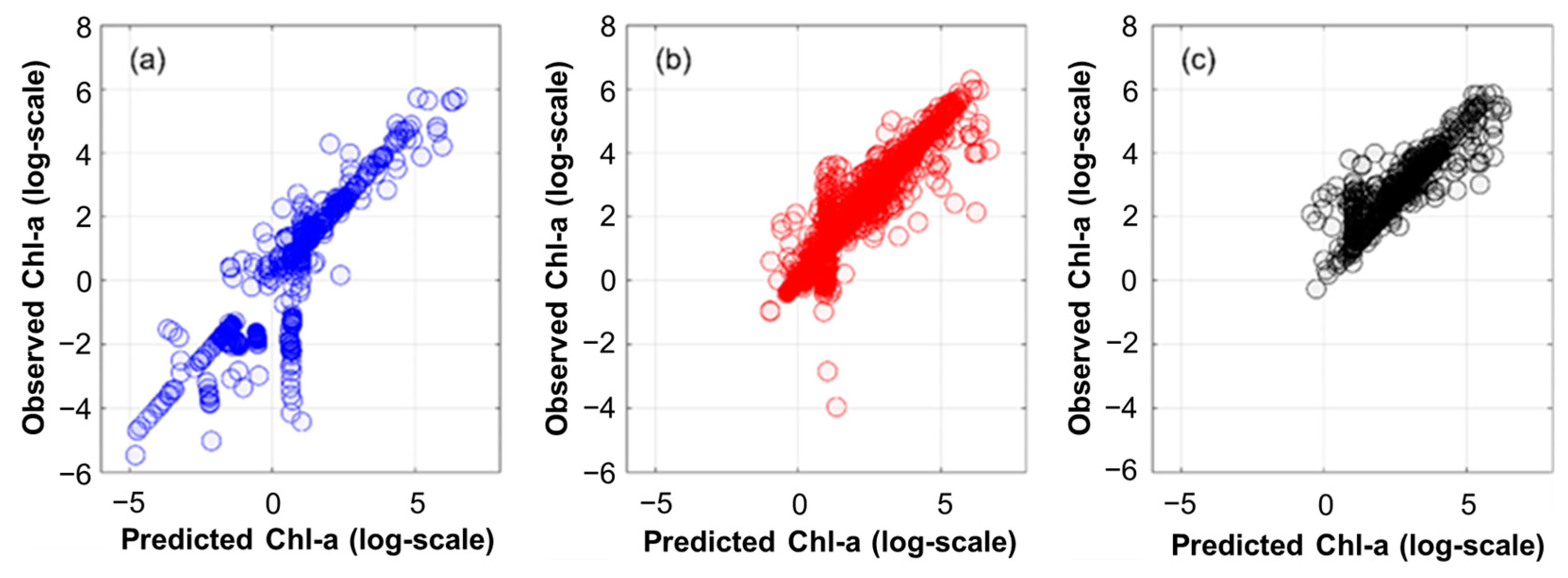
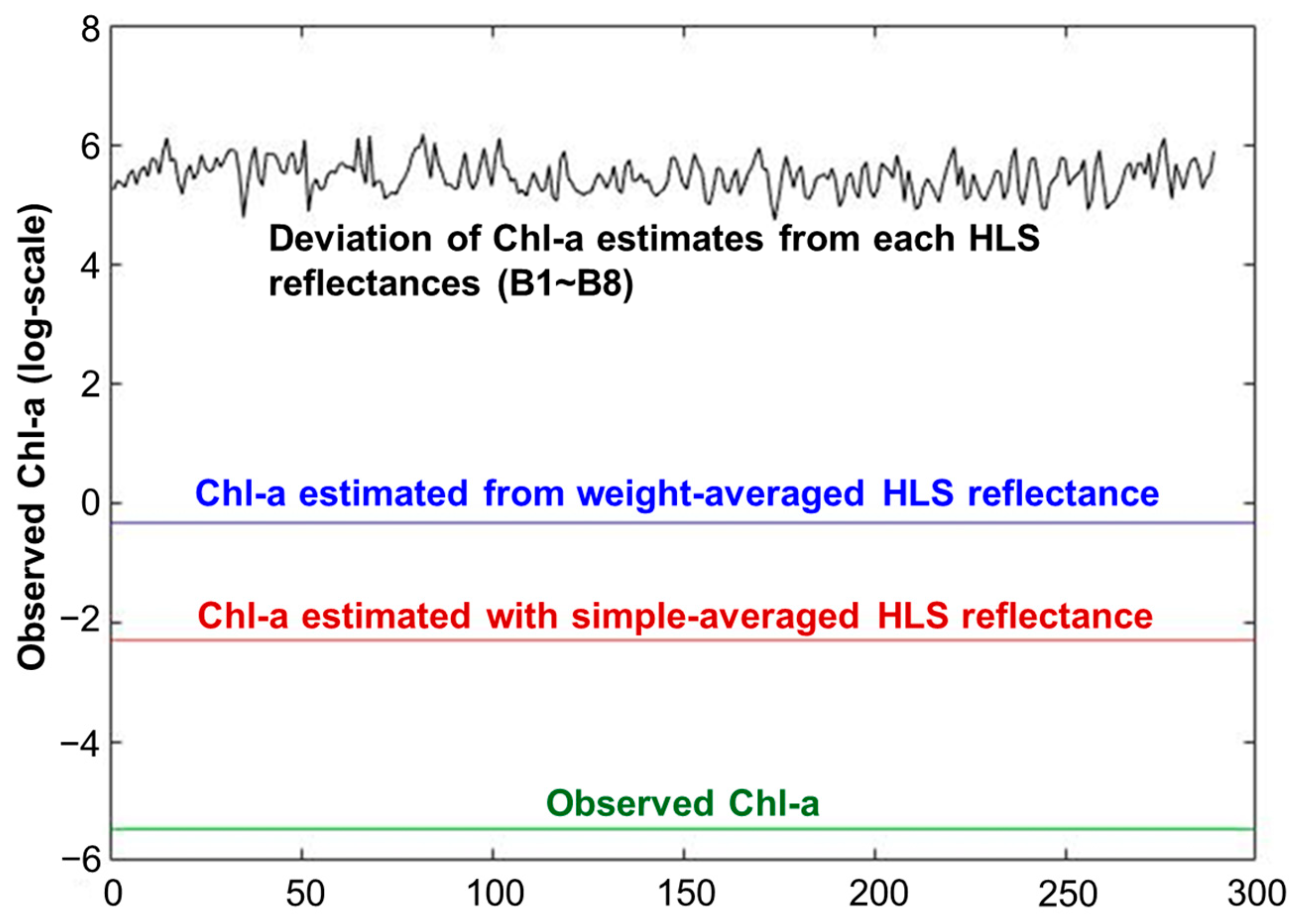
Figure 6 represents the scatterplot of observed versus estimated Chl-a from AIC-like weighted regression for spring (March to May), summer (June to August), and autumn (September to November). The R2 values ranged from 0.89 to 0.93, indicating that the estimated Chl-a showed good consistency with the observed Chl-a across all seasons. In terms of bias and RMSE, summer had the lowest bias (0.06 µg/L) and RMSE (0.55 µg/L), followed by autumn (bias: 0.20 µg/L, RMSE: 0.89 µg/L) and spring (bias: −0.39 µg/L, RMSE: 1.08 µg/L). One of the main reasons for the relatively poorer statistical performance during spring is the presence of a strong vertical line in Figure 6a, along with a scattered pattern at relatively low Chl-a concentrations. Similar findings have been reported by Seegers et al. [52] and Neil et al. [53], indicating that Chl-a estimated via satellite-based band reflectance exhibited lower statistical performance in the low Chl-a concentration range. Figure 7 depicts a typical example of the Chl-a estimation process by an AIC-like weighted scheme over the spring period. Specifically, Chl-a estimates from each HLS reflectance (before averaging each band spectrum) yielded a large deviation from the observed Chl-a. This phenomenon occurred due to the small magnitude (ranging from 1.9 × 10⁻⁶ to 8.7 × 10⁻⁶) and variation in reflectance (ranging from 10−6 to 10−5) within spatio-temporal windows. These band reflectances are used as independent variables for the simple linear equation developed with the n-1 combination of matchup pairs, which creates a large deviation from the Chl-a observation. In the case of Chl-a estimates with simple-averaged reflectance, it yielded relatively less deviation with the measurement than weight-averaged HLS reflectance. Consequently, even though AIC-based weights are continuously updated during iterations, they may not be updated significantly if the band reflectance does not vary. The main reason for the small magnitude and variation is related to the different characteristics of satellite-based reflectance depending on the water body condition. In general, scattering in water is caused by pigments and other impurities, contributing to the overall reflectance. Conversely, clean water yields a low signal-to-noise ratio across the visible and near-infrared spectrum as it acts as an absorber [54]. In addition, Timmons [55] revealed that inland lakes over Ohio during spring are under well-mixed conditions due to the spring turnover, leading to homogeneous water conditions and small magnitude and variation in satellite-based reflectance.

4.3. Influence of the Spatial and Temporal Windows on Estimating Chlorophyll-a

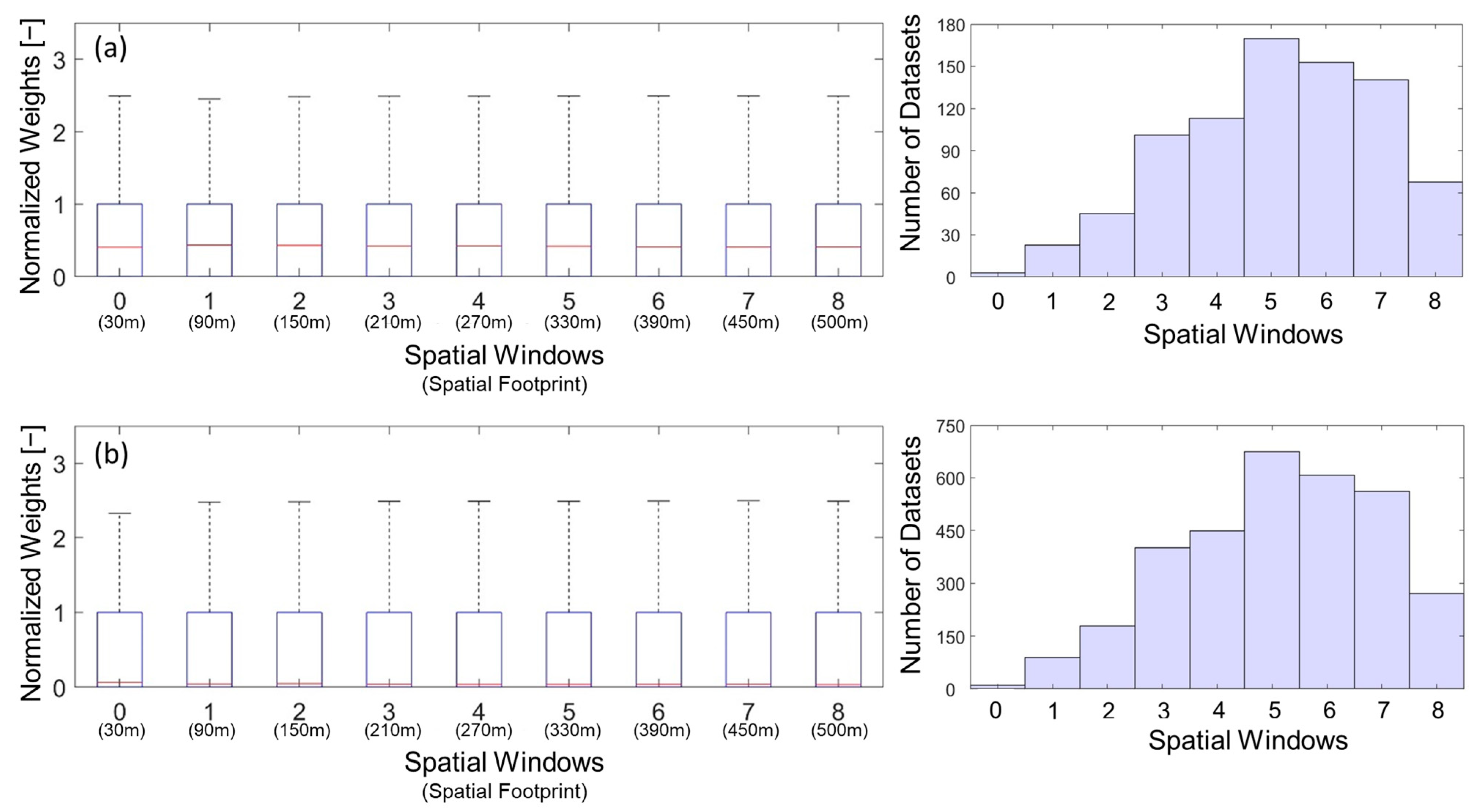
This section focuses on analyzing the overall influence of spatial and temporal windows (depicted in Section 3.3) on the estimation of chlorophyll-a using AIC-like weighted regression. Figure 8 illustrates the boxplots of the normalized weight across different spatial windows for Lake Erie and the other inland lakes. For Lake Erie, the median normalized weight varied from 0.405 to 0.433, while the mean normalized weight tended to increase with the expansion of the spatial window from 0.696 (zero spatial window) to 1.152 (eight-pixel spatial window). Sayers et al. [56] explored the spatial and temporal heterogeneity of water quality parameters and their optical properties during 2015–2016. The results indicated that the normalized beam attenuation and scattering coefficients from the stations located within 13 km showed similar magnitudes, even though the water quality indicators revealed slightly different values. This suggests that expanding the spatial window over Lake Erie could help acquire more available band reflectance, thereby resulting in more accurate Chl-a estimation. For all inland lakes except Lake Erie, the median normalized weight ranged from 0.037 to 0.065, which was significantly less than that from Lake Erie. Fee et al. [57] suggested that the spatial gradient of nutrient concentration in a smaller lake was significantly smaller than that in a relatively larger lake due to the difference in the mixing layer. On the other hand, the mean normalized weight for other lakes suggested that the band reflectance extracted at a point (zero spatial window) revealed the highest mean normalized weight of 2.085. This phenomenon can be explained by the fact that a large spatial window can introduce the uncertainty caused by the land vegetation surrounding lakes.
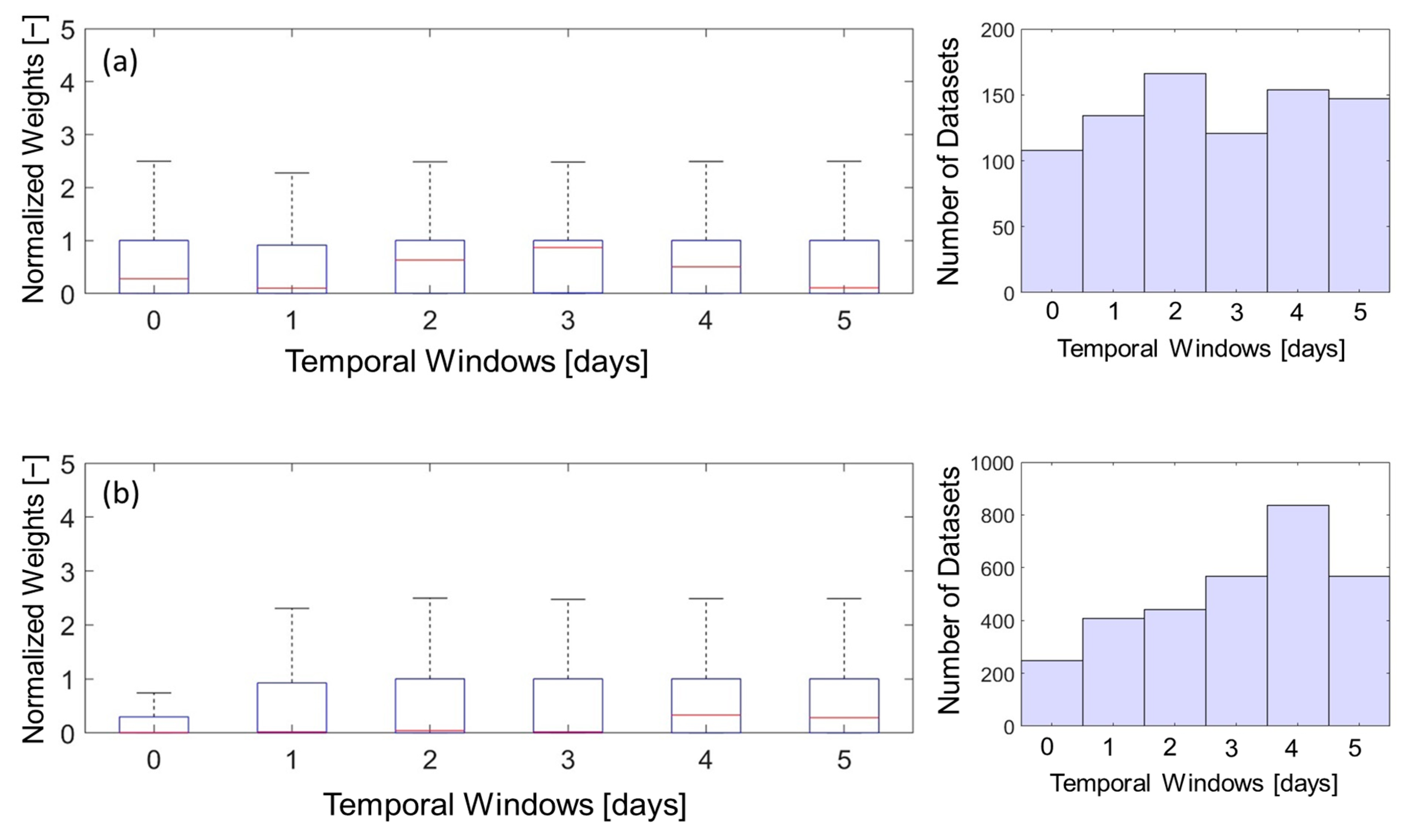
According to Figure 9, temporal windows of ±3 days and ±4 days yielded the largest median normalized weights across Lake Erie and the other inland lakes, respectively. In the case of exact same-day matches and a temporal window of ±1 day, relatively small median normalized weights were observed across all lakes. In terms of mean normalized weight, all lakes revealed the highest mean values at a temporal window of ±3 days, followed by ±2 days and ±1 day. The main reason for the relatively small weight given to the exact same-day match observations was the insufficient number of datasets compared to other temporal windows. For instance, the number of cloud-free HLS images matched with ground-based records during the study period was less than 150, while this number tripled when the temporal window was extended to ±3 days over Lake Erie.
Several researchers have explored effective time windows for applying satellite observations to estimate Chl-a. For example, Balley and Werdall [58] suggested to utilize a 3-h time difference between satellite-based imagery and ground-based measurements to estimate accurate water quality parameters. Conversely, Li et al. [59] used temporal windows of ±7 days and ±12 days to estimate Chl-a over Chinese lakes in the northern and southern parts of the country, respectively, using support vector machines. Kayastha et al. [38] explored effective time windows (up to ±5 days) for Landsat-5, Landsat-8, and Sentinel-2 to estimate Chl-a over Oklahoma reservoirs from 2006 to 2020. Their results indicated that Landsat-5 yielded the best statistical performance in a relatively short temporal window (±1 day), while Landsat-8 and Sentinel-2 yielded the best coefficients of determination with temporal windows of ±3 days and ±5 days, respectively. It is worth noting that the average cloud cover over the state of Ohio falls within 60 to 70%, with Lake Erie generally showing cloud cover over 60% excluding the summer season over the past 30 years [60]. Consequently, the appearance of relatively high cloud cover hinders the acquisition of cloud-free satellite images and reduces the available number of datasets to estimate Chl-a. This suggests that extending the temporal windows could help secure sufficient datasets to estimate Chl-a over inland lakes across Ohio.

5. Conclusions

This study proposed a novel, simple AIC-like weighted regression method for estimating Chl-a using band reflectance observed from HLS and applied it to inland lakes in Ohio. Prior analysis of the temporal behavior of Chl-a across these lakes revealed that the maximum Chl-a concentration was observed during the 2015–2016 seasons, with the highest concentrations measured in major inland lakes such as Grand Lake St. Marys (GLSM) and Buckeye Lake. For Lake Erie, there was a significant difference in Chl-a concentration before and after 2010.
Chl-a concentration was then estimated using cloud-free HLS imagery over Ohio and an AIC-like weighted regression scheme. The statistical evaluation confirmed that Chl-a estimated from AIC-like weighted regression (R2 = 0.92, σ E 2 = 0.31 µg/L) yielded significantly better statistics than both multivariate linear regression (R2 = 0.34, σ E 2 = 2.34 µg/L) and random forest (R2 = 0.82, σ E 2 = 0.92 µg/L). In terms of seasonal analysis, the summer and autumn seasons revealed good statistical performance, while the spring season showed the poorest performance due to relatively small variations in band reflectance caused by large scattering components over deep water and low Chl-a concentrations in spring.
Further analysis of the weight depending on different spatial window length revealed that spatial homogeneity was high for both Lake Erie and the other inland lakes. However, the mean normalized weight suggested that the expansion of the spatial window should be carefully chosen depending on the lake size and surrounding vegetation. In terms of temporal windows, ±2, ±3, and ±4 days yielded the highest weights over inland lakes in Ohio. This indicates that increasing the temporal window up to 4 days helps acquire a sufficient number of datasets to estimate Chl-a without impeding the underlying assumption of relatively homogeneous temporal variations in inland lake water quality.
The AIC-like weighted regression method proposed in this study can be further examined by using band reflectance from different optical sensors and applying it to various water quality parameters (e.g., nutrients, Secchi depth, and organic matter) as well as hydrometeorological variables (e.g., land surface temperature and soil moisture). For future studies, consideration of water reflectance by using open-water-based atmospheric corrections (e.g., Atmospheric Correction for OLI, Case 2 Regional CoastColour) can be applied to retrieve water quality parameters from optical imagery. Additionally, the AIC-like weighted regression method can be improved by implementing different weighting schemes depending on the size of the lake and the influence of different seasons.

Author Contributions

Conceptualization, J.P., K.Z. and S.K.; methodology, J.P., K.Z. and S.K.; validation, J.P.; formal analysis, J.P., K.Z., S.K. and K.B.; investigation, J.P., K.Z., S.K. and K.B.; data curation, J.P. and K.Z.; writing—original draft preparation, J.P., K.Z., S.K. and K.B.; writing—review and editing, J.P., K.Z., S.K. and K.B.; visualization, J.P.; supervision, K.Z., K.B. and S.K.; funding acquisition, J.P. All authors have read and agreed to the published version of the manuscript.

Funding

This study was supported by Korea National University of Transportation Industry-Academy Cooperation Foundation in 2023.

Data Availability Statement

The ground-based Chl-a measurements managed by National Water Information Service, Sustaining the Earth’s Watersheds, Agricultural Research Data System, and STOrage and Retrieval (STORET) data utilized in this study can be obtained through the National Water Quality Council (https://waterqualitydata.us, accessed on 28 May 2022). Water quality parameters acquired from Ohio Sea Grant and Stone Laboratory can be retrieved through Stone Lab Algal and Water Quality Laboratory (https://ohioseagrant.osu.edu/research/live/water, accessed on 17 April 2022). Datasets measured by Great Lake Environmental Research Laboratory are publicly available through the NOAA GLERL webpage (https://www.glerl.noaa.gov/data/#biological, accessed on 31 May 2024). AquaSat dataset can be found via the University of North Carolina, Chapel Hill Global Hydrology Lab github (https://www.glerl.noaa.gov/data/#biological, accessed on 10 May 2022). Harmonized Landsat Sentinel-2 dataset is publicly available through NASA EarthData (https://earthdata.nasa.gov, accessed on 21 May 2022; DOI: 10.5067/HLS/HLSL30).

Acknowledgments

The authors appreciate Xuesong Zhang at USDA-ARS, Alexis Londo at the Ohio State University, Joshi Neha at Arcadis U.S., Inc., the Harmful Algal Bloom Research Initiative of the Ohio Department of Higher Education, and two anonymous reviewers.

Conflicts of Interest

The authors declare no conflicts of interest.

References

  1. Griffith, A.W.; Gobler, C.J. Harmful algal blooms: A climate change co-stressor in marine and freshwater ecosystems. Harmful Algae 2020, 91, 101590. [Google Scholar] [CrossRef] [PubMed]
  2. Hallegraeff, G.M.; Anderson, D.M.; Belin, C.; Bottein, M.Y.D.; Bresnan, E.; Chinain, M.; Enevoldsen, H.; Iwataki, M.; Karlson, B.; McKenzie, C.H.; et al. Perceived global increase in algal blooms is attributable to intensified monitoring and emerging bloom impacts. Commun. Earth Environ. 2021, 2, 117. [Google Scholar] [CrossRef] [PubMed]
  3. Zhang, J.; Phaneuf, D.J.; Schaeffer, B.A. Property values and cyanobacterial algal blooms: Evidence from satellite monitoring of Inland Lakes. Ecol. Econ. 2022, 199, 107481. [Google Scholar] [CrossRef]
  4. Tanvir, R.U.; Hu, Z.; Zhang, Y.; Lu, J. Cyanobacterial community succession and associated cyanotoxin production in hypereutrophic and eutrophic freshwaters. Environ. Pollut. 2021, 290, 118056. [Google Scholar] [CrossRef]
  5. Schreidah, C.M.; Ratnayake, K.; Senarath, K.; Karunarathne, A. Microcystins: Biogenesis, toxicity, analysis, and control. Chem. Res. Toxicol. 2020, 33, 2225–2246. [Google Scholar] [CrossRef] [PubMed]
  6. Hollister, J.W.; Kreakie, B.J. Associations between chlorophyll a and various microcystin health advisory concentrations. F1000Research 2016, 5, 151. [Google Scholar]
  7. He, J.; Chen, Y.; Wu, J.; Stow, D.A.; Christakos, G. Space-time chlorophyll-a retrieval in optically complex waters that accounts for remote sensing and modeling uncertainties and improves remote estimation accuracy. Water Res. 2020, 171, 115403. [Google Scholar] [CrossRef]
  8. Ma, A.Q.; Yan, X.; Wang, Y.X. Research on Remote Sensing Retrieval of Chl-a Concentration in the Jiaozhou Bay, Qingdao Based on Semi-analytical/Semi-empirical Model. In Proceedings of the 2022 3rd International Conference on Geology, Mapping and Remote Sensing (ICGMRS), Zhoushan, China, 22–24 April 2022. [Google Scholar]
  9. Boucher, J.; Weathers, K.C.; Norouzi, H.; Steele, B. Assessing the effectiveness of Landsat 8 chlorophyll a retrieval algorithms for regional freshwater monitoring. Ecol. Appl. 2018, 28, 1044–1054. [Google Scholar] [CrossRef]
  10. Zhang, F.; Li, J.; Yan, B.; Yu, J.; Wang, C.; Wang, S.; Shen, Q.; Wu, Y.; Zhang, B. Tracking historical chlorophyll-a change in the guanting reservoir, Northern China, based on landsat series inter-sensor normalization. Int. J. Remote Sens. 2021, 42, 3918–3937. [Google Scholar] [CrossRef]
  11. Mamun, M.; Ferdous, J.; An, K.G. Empirical estimation of nutrient, organic matter and algal chlorophyll in a drinking water reservoir using Landsat 5 TM data. Remote Sen. 2021, 13, 2256. [Google Scholar] [CrossRef]
  12. Germán, A.; Shimoni, M.; Beltramone, G.; Rodríguez, M.I.; Muchiut, J.; Bonansea, M.; Scavuzzo, C.M.; Ferral, A. Space-time monitoring of water quality in an eutrophic reservoir using Sentinel-2 data-A case study of San Roque, Argentina. Remote Sens. Appl. Soc. Environ. 2021, 24, 100614. [Google Scholar] [CrossRef]
  13. Sherman, J.; Tzortziou, M.; Turner, K.J.; Goes, J.; Grunert, B. Chlorophyll dynamics from Sentinel-3 using an optimized algorithm for enhanced ecological monitoring in complex urban estuarine waters. Int. J. Appl. Earth Obs. Geoinf. 2023, 118, 103223. [Google Scholar] [CrossRef]
  14. Tran, M.D.; Vantrepotte, V.; Loisel, H.; Oliveira, E.N.; Tran, K.T.; Jorge, D.; Mériaux, X.; Paranhos, R. Band Ratios Combination for Estimating Chlorophyll-a from Sentinel-2 and Sentinel-3 in Coastal Waters. Remote Sens. 2023, 15, 1653. [Google Scholar] [CrossRef]
  15. Joshi, N.; Park, J.; Zhao, K.; Londo, A.; Khanal, S. Monitoring Harmful Algal Blooms and Water Quality Using Sentinel-3 OLCI Satellite Imagery with Machine Learning. Remote Sens. 2024, 16, 2444. [Google Scholar] [CrossRef]
  16. Gidudu, A.; Letaru, L.; Kulabako, R.N. Empirical modeling of chlorophyll a from MODIS satellite imagery for trophic status monitoring of Lake Victoria in east Africa. J. Gt. Lakes Res. 2021, 47, 1209–1218. [Google Scholar] [CrossRef]
  17. Mohebzadeh, H.; Mokari, E.; Daggupati, P.; Biswas, A. A machine learning approach for spatiotemporal imputation of MODIS chlorophyll-a. Int. J. Remote Sens. 2021, 42, 7381–7404. [Google Scholar] [CrossRef]
  18. Yu, X.; Shen, J.; Zheng, G.; Du, J. Chlorophyll-a in Chesapeake Bay based on VIIRS satellite data: Spatiotemporal variability and prediction with machine learning. Ocean. Model. 2022, 180, 102119. [Google Scholar] [CrossRef]
  19. Cao, Z.; Ma, R.; Pahlevan, N.; Liu, M.; Melack, J.M.; Duan, H.; Xue, K.; Shen, M. Evaluating and Optimizing VIIRS Retrievals of Chlorophyll-a and Suspended Particulate Matter in Turbid Lakes Using a Machine Learning Approach. IEEE Trans. Geosci. Remote Sens. 2022, 60, 4211417. [Google Scholar] [CrossRef]
  20. Hyde, K.; O’Reilly, J.; Oviatt, C. Validation of SeaWiFS chlorophyll-a in Massachusetts Bay. Cont. Shelf Res 2007, 27, 1677–1691. [Google Scholar] [CrossRef]
  21. Salama, M.S.; Su, Z. Resolving the subscale spatial variability of apparent and inherent optical properties in ocean color match-up sites. IEEE Trans. Geosci. Remote Sens. 2011, 49, 2612–2622. [Google Scholar] [CrossRef]
  22. Carmello, V. Using a spatial synoptic classification to analyze the weather-type dring the main soybean development period in northwest Ohio, 1999–2013. Pa. Geogr. 2019, 57, 34. [Google Scholar]
  23. Urquhart, E.; Schaeffer, B.A.; Stumpf, R.P.; Loftin, K.A.; Werdell, P.J. A method for examining temporal changes in cyanobacterial harmful algal bloom spatial extent using satellite remote sensing. Harmful Algae 2017, 67, 144–152. [Google Scholar] [CrossRef] [PubMed]
  24. Evrendilek, F.; Wali, M.K. Modelling long-term C dynamics in croplands in the context of climate change: A case study from Ohio. Environ. Model. Softw. 2001, 16, 361–375. [Google Scholar] [CrossRef]
  25. Gorham, T.; Jia, Y.; Shum, C.K.; Lee, J. Ten-year survey of cyanobacterial blooms in Ohio’s waterbodies using satellite remote sensing. Harmful Algae 2017, 66, 13–19. [Google Scholar] [CrossRef] [PubMed]
  26. Clark, J.M.; Schaeffer, B.A.; Darling, J.A.; Urquhart, E.A.; Johnston, J.M.; Ignatius, A.R.; Myer, M.H.; Loftin, K.A.; Werdell, P.J.; Stumpf, R.P. Satellite monitoring of cyanobacterial harmful algal bloom frequency in recreational waters and drinking water sources. Ecol. Indic. 2017, 80, 84–95. [Google Scholar] [CrossRef] [PubMed]
  27. Steffen, M.M.; Zhu, Z.; McKay, R.M.L.; Wilhelm, S.W.; Bullerjahn, G.S. Taxonomic assessment of a toxic cyanobacteria shift in hypereutrophic Grand Lake St. Marys (Ohio, USA). Harmful Algae 2014, 33, 12–18. [Google Scholar] [CrossRef]
  28. Mitsch, W.J. Solving Lake Erie’s harmful algal blooms by restoring the Great Black Swamp in Ohio. Ecol. Eng. 2017, 108, 406–413. [Google Scholar] [CrossRef]
  29. Cousino, L.K.; Becker, R.H.; Zmijewski, K.A. Modeling the effects of climate change on water, sediment, and nutrient yields from the Maumee River watershed. J. Hydrol. Reg. Stud. 2015, 4, 762–775. [Google Scholar] [CrossRef]
  30. Philpott, T. The Big-Ag-Fueled Algae Bloom That Won’t Leave Toledo’s Water Supply Alone. Mother Jones. 5 August 2015. Available online: https://www.motherjones.com/food/2015/08/giant-toxic-algae-bloom-haunts-toledo/#:~:text=The%20citizens%20of%20Toledo%2C%20Ohio,400%2C000%20draws%20its%20tap%20water (accessed on 5 May 2024).
  31. Wurtsbaugh, W.A.; Paerl, H.W.; Dodds, W.K. Nutrients, eutrophication and harmful algal blooms along the freshwater to marine continuum. Wiley Inerdiscip. Rev. Water 2019, 6, e1373. [Google Scholar] [CrossRef]
  32. Ross, M.R.; Topp, S.N.; Appling, A.P.; Yang, X.; Kuhn, C.; Butman, D.; Simard, M.; Pavelsky, T.M. AquaSat: A data set to enable remote sensing of water quality for inland waters. Water Resour. Res. 2019, 55, 10012–10025. [Google Scholar] [CrossRef]
  33. Chaffin, J.D.; Kane, D.D.; Stanislawczyk, K.; Parker, E.M. Accuracy of data buoys for measurement of cyanobacteria, chlorophyll, and turbidity in a large lake (Lake Erie, North America): Implications for estimation of cyanobacterial bloom parameters from water quality sonde measurements. Environ. Sci. Pollut. Res. 2018, 25, 25175–25189. [Google Scholar] [CrossRef] [PubMed]
  34. Cooperative Institute for Great Lakes Research; University of Michigan and NOAA Great Lakes Environmental Research Laboratory. Physical, Chemical, and Biological Water Quality Monitoring Data to Support Detection of Harmful Algal Blooms (HABs) in Western Lake Erie, Collected by the Great Lakes Environmental Research Laboratory and the Cooperative Institute for Great Lakes Research Since 2012; [2015–2017]; NOAA National Centers for Environmental Information: Asheville, NC, USA, 2019. [Google Scholar] [CrossRef]
  35. Hoffman, D.K.; McCarthy, M.J.; Boedecker, A.R.; Myers, J.A.; Newell, S.E. The role of internal nitrogen loading in supporting non-N-fixing harmful cyanobacterial blooms in the water column of a large eutrophic lake. Limnol. Oceanogr. 2022, 67, 2028–2041. [Google Scholar] [CrossRef]
  36. Claverie, M.; Ju, J.; Masek, J.G.; Dungan, J.L.; Vermote, E.F.; Roger, J.C.; Skakun, S.V.; Justice, C. The Harmonized Landsat and Sentinel-2 surface reflectance data set. Remote Sens. Environ. 2018, 219, 145–161. [Google Scholar] [CrossRef]
  37. Claverie, M.; Masek, J.G.; Ju, J.; Dungan, J.L. Harmonized Landsat-8 Sentinel-2 (HLS) Product User’s Guide; National Aeronautics and Space Administration (NASA): Washington, DC, USA, 2017. [Google Scholar]
  38. Kayastha, P.; Dzialowski, A.R.; Stoodley, S.H.; Wagner, K.L.; Mansaray, A.S. Effect of time window on satellite and ground-based data for estimating chlorophyll-a in reservoirs. Remote Sens. 2022, 14, 846. [Google Scholar] [CrossRef]
  39. Liu, X.; Yang, Q.; Wang, Y.; Zhang, Y. Evaluation of GOCI remote sensing reflectance spectral quality based on a quality assurance score system in the Bohai Sea. Remote Sens. 2022, 14, 1075. [Google Scholar] [CrossRef]
  40. Zhang, M.; Ibrahim, A.; Franz, B.A.; Ahmad, Z.; Sayer, A.M. Estimating pixel-level uncertainty in ocean color retrievals from MODIS. Opt. Express 2022, 30, 31415–31438. [Google Scholar] [CrossRef] [PubMed]
  41. Zhou, Y.; Yu, D.; Cheng, W.; Gai, Y.; Yao, H.; Yang, L.; Pan, S. Monitoring multi-temporal and spatial variations of water transparency in the Jiaozhou Bay using GOCI data. Mar. Pollut. Bull. 2022, 180, 113815. [Google Scholar] [CrossRef] [PubMed]
  42. Keith, D.; Rover, J.; Green, J.; Zalewsky, B.; Charpentier, M.; Thursby, G.; Bishop, J. Monitoring algal blooms in drinking water reservoirs using the Landsat-8 Operational Land Imager. Int. J. Remote Sens. 2018, 39, 2818–2846. [Google Scholar] [CrossRef]
  43. McCullough, I.M.; Loftin, C.S.; Sader, S.A. Combining lake and watershed characteristics with Landsat TM data for remote estimation of regional lake clarity. Remote Sens. Environ. 2012, 123, 109–115. [Google Scholar] [CrossRef]
  44. Mishra, D.R.; Narumalani, S.; Rundquist, D.; Lawson, M. Characterizing the vertical diffuse attenuation coefficient for downwelling irradiance in coastal waters: Implications for water penetration by high resolution satellite data. ISPRS J. Photogramm. Remote Sens. 2005, 60, 48–64. [Google Scholar] [CrossRef]
  45. Vehtari, A.; Gelman, A.; Gabry, J. Practical Bayesian model evaluation using leave-one-out cross-validation and WAIC. STAT Comput. 2017, 27, 1413–1432. [Google Scholar] [CrossRef]
  46. Carlson, R.E. A coordinator’s guide to volunteer lake monitoring methods. N. Am. Lake Manag. Soc. 1996, 96, 305. [Google Scholar]
  47. Hoorman, J.; Hone, T.; Sudman Jr, T.; Dirksen, T.; Iles, J.; Islam, K.R. Agricultural impacts on lake and stream water quality in Grand Lake St. Marys, Western Ohio. Water Air Soil Pollut. 2008, 193, 309–322. [Google Scholar] [CrossRef]
  48. Perry Soil and Water Conservation District. Buckeye Lake HUC-12: Nine Element Nonpoint Source Implementation Strategic Plan (NPS-IS Plan); Perry Soil and Water Conservation District: Somerset, OH, USA, 2020. [Google Scholar]
  49. Michalak, A.M.; Anderson, E.J.; Beletsky, D.; Boland, S.; Bosch, N.S.; Bridgeman, T.B.; Chaffin, J.D.; Cho, K.; Confesor, R.; Daloglu, I.; et al. Record-setting algal bloom in Lake Erie caused by agricultural and meteorological trends consistent with expected future conditions. Proc. Natl. Acad. Sci. USA 2013, 110, 6448–6452. [Google Scholar] [CrossRef] [PubMed]
  50. Kraemer, B.M.; Mehner, T.; Adrian, R. Reconciling the opposing effects of warming on phytoplankton biomass in 188 large lakes. Sci. Rep. 2017, 7, 10762. [Google Scholar] [CrossRef]
  51. Smith, D.R.; King, K.W.; Williams, M.R. What Is Causing the Harmful Algal Blooms in Lake Erie? J. Soil Water Conserv. 2015, 70, 27A–29A. [Google Scholar] [CrossRef]
  52. Seegers, B.N.; Werdell, P.J.; Vandermeulen, R.A.; Salls, W.; Stumpf, R.P.; Schaeffer, B.A.; Owens, T.J.; Bailey, S.W.; Scott, J.P.; Loftin, K.A. Satellites for Long-Term Monitoring of Inland U.S. Lakes: The MERIS Time Series and Application for Chlorophyll-A. Remote Sens. Environ. 2021, 266, 112685. [Google Scholar] [CrossRef]
  53. Neil, C.; Spyrakos, E.; Hunter, P.D.; Tyler, A.N. A global approach for chlorophyll-a retrieval across optically complex inland waters based on optical water types. Remote Sens. Environ. 2019, 229, 159–178. [Google Scholar] [CrossRef]
  54. Zeng, C.; Richardson, M.; King, D.J. The impacts of environmental variables on water reflectance measured using a lightweight unmanned aerial vehicle (UAV)-based spectrometer system. ISPRS J. Photogramm. Remote Sens. 2017, 130, 217–230. [Google Scholar] [CrossRef]
  55. Timmons, J.S. Identifying the Isotopic Signature of Lake Effect Precipitation on Northeast Ohio Isocape. Master’s Thesis, Kent State University, Kent, OH, USA, 2021. [Google Scholar]
  56. Sayers, M.J.; Bosse, K.R.; Shuchman, R.A.; Ruberg, S.A.; Fahnenstiel, G.L.; Leshkevich, G.A.; Stuart, D.G.; Johengen, T.H.; Burtner, A.M.; Palladino, D. Spatial and temporal variability of inherent and apparent optical properties in western Lake Erie: Implications for water quality remote sensing. J. Gt. Lakes Res. 2019, 45, 490–507. [Google Scholar] [CrossRef]
  57. Fee, E.J.; Hecky, R.E.; Regehr, G.W.; Hendzel, L.L.; Wikinson, P. Effects of lake size on nutrient availability in the mixed layer during summer stratification. Can. J. Fish. Aquat. Sci. 1994, 52, 2756–2768. [Google Scholar] [CrossRef]
  58. Bailey, S.W.; Werdell, P. A multi-sensor approach for the on-orbit validation of ocean color satellite data products. Remote Sens. Environ. 2006, 102, 12–23. [Google Scholar] [CrossRef]
  59. Li, S.; Song, K.; Wang, S.; Liu, G.; Wen, Z.; Shang, Y.; Lyu, L.; Chen, F.; Xu, S.; Tao, H.; et al. Quantification of chlorophyll-a in typical lakes across China using Sentinel-2 MSI imagery with machine learning algorithm. Sci. Total Environ. 2021, 778, 146271. [Google Scholar] [CrossRef]
  60. Ackerman, S.A.; Heidinger, A.; Foster, M.J.; Maddux, B. Satellite regional cloud climatology over the Great Lakes. Remote Sens. 2013, 5, 6223–6240. [Google Scholar] [CrossRef]
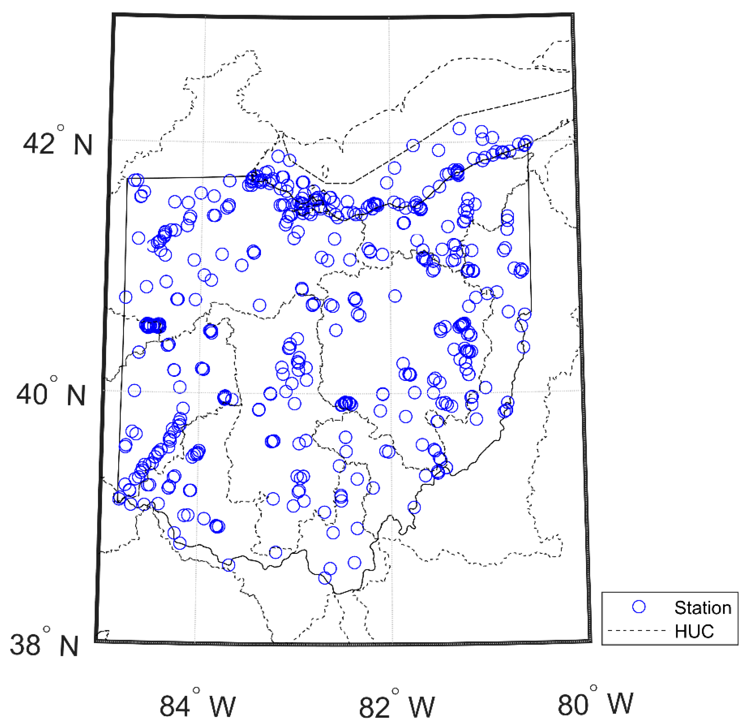
Figure 1. Geographic information of the study area. The blue dots represent the ground-based stations utilized in this study, and the dotted line delineates the boundary of the Hydrologic Unit Code (HUC)-4.
Remotesensing 16 02761 g001
Figure 2. Overall framework of the proposed AIC-like weighted linear regression model.
Remotesensing 16 02761 g002
Figure 3. (a) Temporal behavior of Chl-a concentration and (b) annually averaged concentration and standard deviation of Chl-a concentration over inland lakes in Ohio.
Remotesensing 16 02761 g003
Figure 4. Temporal variation in chlorophyll-a concentration over Lake Erie (a) from 2000 to 2009 and (b) 2010 to 2020.
Remotesensing 16 02761 g004
Figure 5. Scatterplot of Chl-a estimates from (a) multivariate regression and (b) AIC-like weighted regression.
Remotesensing 16 02761 g005
Figure 6. Seasonal scatterplot of observed and predicted Chl-a during (a) spring, (b) summer, and (c) autumn.
Remotesensing 16 02761 g006
Figure 7. Example of Chl-a estimation with AIC-like weighted scheme over spring period.
Remotesensing 16 02761 g007
Figure 8. Boxplot of weight depending on different spatial windows along with number of datasets used for (a) Lake Erie and (b) other inland lakes across Ohio.
Remotesensing 16 02761 g008
Figure 9. Boxplot of weight depending on different temporal windows for (a) Lake Erie and (b) other inland lakes across Ohio.
Remotesensing 16 02761 g009
Table 1. Spectral characteristics of the Harmonized Landsat and Sentinel-2 (HLS) datasets.
Band NameWavelength (μm)Landsat 8Sentinel-2
Costal Aerosol0.43–0.45Band 01B01
Blue0.45–0.51Band 02B02
Green0.53–0.59Band 03B03
Red0.64–0.67Band 04B04
NIR narrow0.85–0.88Band 05B8A
SWIR 1 11.57–1.65Band 06B11
SWIR 22.11–2.29Band 07B12
Cirrus1.36–1.38Band 09B10
1 Shortwave infrared.
Disclaimer/Publisher’s Note: The statements, opinions and data contained in all publications are solely those of the individual author(s) and contributor(s) and not of MDPI and/or the editor(s). MDPI and/or the editor(s) disclaim responsibility for any injury to people or property resulting from any ideas, methods, instructions or products referred to in the content.