A Novel Modified Symmetric Nested Array for Mixed Far-Field and Near-Field Source Localization

Abstract

In the process of locating mixed far-field and near-field sources, sparse nonlinear arrays (SNAs) can achieve larger array apertures and higher degrees of freedom compared to traditional uniform linear arrays (ULAs) with the same number of sensors. This paper introduces a Modified Symmetric Nested Array (MSNA), which can automatically generate the optimal array structure with the maximum continuous lags for a given number of sensors. To effectively address mixed source localization, we designed an estimation algorithm based on high-order cumulants and the subarray partition method, applied to the MSNA. Firstly, a specialized fourth-order cumulant matrix, relevant only to Direction of Arrival (DOA) information, is constructed for the DOA estimation of mixed sources. Then, peak searching using the estimated DOA information enables the estimation of the distance parameters, effectively separating mixed sources. The algorithm has moderate computational complexity and provides high resolution and estimation accuracy. Numerical simulation results demonstrate that, with the same number of physical sensors, the proposed MSNA provides more continuous lags than existing arrays, offering higher degrees of freedom and estimation accuracy.

1. Introduction

Mixed source localization has been a highly researched area in the fields of communication and signal processing. Its significant application value is evident in various domains such as radar, seismic surveying, sonar, wireless communication, microphone-array-based speech localization, etc. [1,2,3,4,5,6,7]. According to the definition of the Fresnel region, signal sources can be classified into far-field sources and near-field sources. When the signal source is significantly beyond the Fresnel region, it is considered a far-field source. In such cases, the signal model can be assumed to be a plane wave model. During the process of signal source localization, only Direction of Arrival (DOA) estimation is required. On the contrary, when the signal source is located within the Fresnel region, it is considered a near-field source. In this scenario, the plane wave assumption becomes invalid, and the signal model for incident waves is represented by spherical waves. The source location is now determined by both angle and distance parameters. Over the past few decades, scholars have conducted in-depth research on both near-field and far-field source localization, proposing a series of algorithms that demonstrate superior performance. Representative algorithms applied to far-field source localization include the MUSIC [8] and ESPRIT [9] algorithms. For near-field source localization, algorithms such as the path-following algorithm [10] and the weighted linear prediction method [11] are commonly used. Based on coherent source localization estimation, scholars have proposed the spatial smoothing algorithm and algorithms based on deep learning [12,13].

The aforementioned algorithms are effective only in scenarios where the signal sources are either purely far-field or purely near-field. They cannot meet the requirements of mixed-field source localization when both far-field and near-field sources coexist. In recent years, due to practical demands in scenarios like microphone array localization [14], an increasing number of researchers have been dedicated to algorithmic research for mixed-field source localization. Liang et al. proposed a two-stage MUSIC algorithm based on fourth-order cumulants [15]. This algorithm addresses the mixed source localization problem by constructing two specific fourth-order cumulant matrices. The fundamental idea is to utilize the information about the DOA of all sources obtained from the first fourth-order cumulant matrix. Subsequently, the second fourth-order cumulant matrix is used to acquire distance information for all sources, thereby distinguishing mixed sources. Building upon second-order cumulants, scholars have proposed the oblique projection algorithm [16,17,18,19]. The key concept behind this algorithm is to suppress the influence of far-field sources in the covariance matrix, thereby eliminating the subspace associated with far-field sources. Consequently, the subspace corresponding to near-field sources is obtained, allowing for the effective separation of mixed sources. In comparison to the two-stage MUSIC algorithm, the oblique projection algorithm can effectively reduce the computational complexity. Yang et al. [20] proposed a low-complexity localization algorithm based on the root-MUSIC theory. By employing polynomial root finding instead of a MUSIC spectrum peak search, the algorithm’s computational complexity is further reduced.

The array aperture plays a crucial role in the performance of source localization. In general, a larger array aperture leads to more accurate estimates of DOAs and distances [21]. However, existing source-localization algorithms are mostly developed based on linear uniform arrays, where the array aperture is proportional to the number of physical sensors. Consequently, the number of consecutive lags is constrained by the physical size of the array elements [22]. To achieve a larger array aperture, more physical sensor resources are required, significantly escalating the cost of array deployment. Fortunately, researchers have developed non-uniform linear array structures that effectively address this issue [23,24,25,26,27,28]. In comparison to uniform linear arrays, nested arrays [29] and coprime arrays [30], proposed by Pal and others, can attain longer consecutive lags and larger array apertures. Meanwhile, signal-processing algorithms for sparse array structures have also been developed by researchers. Zhou et al. [31] propose a novel sparse array DOA estimation algorithm via structured correlation reconstruction. By filling presumed sensors on the missing Nyquist sampling positions, the array’s degrees of freedom can be fully utilized, offering greater flexibility in array configuration constraints. Zheng et al. [32] propose a coarray tensor DOA estimation algorithm. This algorithm is based on the cross-correlation tensor between sub-Nyquist tensor signals and can effectively enhance the array’s source identification capability. Although the above algorithms significantly enhance the estimation capability of sparse arrays, they are designed for purely far-field or purely near-field signals and lack the ability to estimate mixed sources.

To address the problem of mixed-field source localization, this paper proposes an MSNA and a corresponding mixed-source-estimation algorithm. The main contributions of this paper are as follows:

(1)

This paper proposes an MSNA and provides its structural formula. The MSNA can achieve a larger array aperture and a longer number of consecutive lags, thereby improving estimation resolution and the array degrees of freedom.

(2)

Based on the subarray partition method and high-order statistics, this paper proposes a dedicated signal processing algorithm for mixed source localization using the MSNA. This algorithm has moderate computational complexity compared to similar algorithms.

(3)

This paper verifies the advantage of the MSNA in terms of degrees of freedom and demonstrates the performance benefits of the estimation algorithm based on the MSNA.

Throughout this paper, the vectors and the matrices are represented by lower-case and upper-case, respectively. $⌈•⌉$ represents round towards infinite, and $⌊•⌋$ represents round towards zero. The superscripts ${\left[•\right]}^T$, ${\left[•\right]}^H$, and ${\left[•\right]}^{*}$ denote the transpose, conjugate transpose, and complex conjugate, respectively. $E(•)$ represents the expectation operation. $cum(•)$ represents the cumulative operation of random variables.

2. Signal Model

Assume there are K narrowband uncorrelated signals incident on the MSNA, which consists of $2M+2N-1$ sensors, as illustrated in Figure 1. The MSNA is composed of 3 subarrays and 2 additional sensor elements, with a minimum inter-sensor spacing of d, where d is a $1/4$ wavelength. Subarray 1 is comprised of $2M+1$ sensors with a spacing of $Nd$. Subarrays 2 and 3 are symmetrical to each other, each consisting of $N-2$ sensors with a spacing of d. They are spaced $2d$ apart from subarray 1. Additionally, two extra sensors are positioned at both ends of the array, with the leftmost sensor spaced $2d$ from subarray 3 and the rightmost sensor spaced $2d$ from subarray 2. In this MSNA array, the sensor indices can be represented as $\left\{-M-N+1,-M-N+2,\cdots ,M+N-2,M+N-1\right\}$. The sensor positions can be represented by the set $\mathbb{D}$.

$$\mathbb{D}=\mathbb{S}·d=\left\{p_{-L}·d,\cdots ,p_0·d,\cdots ,p_L·d\right\}$$

(1)

where $\mathbb{S}=\left\{p_{-L},\cdots ,p_0,\cdots ,p_L\right\}$ and $L=M+N-1$ and the position of the ith sensor is denoted as $p_i·d$, $i\in [-L,-L+1,\cdots ,L-1,L]$. The set $\mathbb{S}$ can be decomposed into five parts, corresponding, respectively, to subarrays 1–3 of the symmetric sparse array and the two additional sensors.

$$\mathbb{S}={\mathbb{S}}_1\cup {\mathbb{S}}_2\cup {\mathbb{S}}_3\cup {\mathbb{S}}_4\cup {\mathbb{S}}_5$$

(2)

where ${\mathbb{S}}_1$, ${\mathbb{S}}_2$, and ${\mathbb{S}}_3$ correspond to subarrays 1–3 and ${\mathbb{S}}_4$ and ${\mathbb{S}}_5$ correspond to the two additional sensors, representing the rightmost and leftmost sensors, respectively. The specific structure is as follows:

$${\mathbb{S}}_1=\left\{p_{i_1}\mid p_{i_1}=N{i}_1,-M\le i_1\le M\right\}$$

(3)

$${\mathbb{S}}_2=\left\{p_{i_2}\mid p_{i_2}=MN-M+i_2+1,M+1\le i_2\le M+N-2\right\}$$

(4)

$${\mathbb{S}}_3=\left\{p_{i_3}\right|p_{i_3}=-MN+M+i_3-1,-M-N+2\le i_3\le -M-1\}$$

(5)

$${\mathbb{S}}_4=\left\{p_{i_4}\right|p_{i_4}=MN+N+1\}$$

(6)

$${\mathbb{S}}_5=\left\{p_{i_5}\right|p_{i_5}=-MN-N-1\}$$

(7)

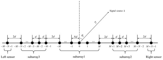
Figure 1. The MSNA geometry.

Assuming the sensor at position 0 serves as the phase reference point, the received signal at the ith sensor at time t can be expressed as [15]:

$$x_i\left(t\right)=\sum _{k=1}^K{s}_k\left(t\right)e^{j{\tau }_{ik}}+n_i\left(t\right)$$

(8)

where $s_k\left(t\right)$ is the kth narrowband signal, $n_i\left(t\right)$ is Gaussian white noise, and ${\tau }_{ik}$ represents the delay (the propagation delay of the kth narrowband signal arriving at the ith sensor relative to the reference sensor at position 0). If the kth signal is a near-field source, it can be specifically expressed as follows:

$${\tau }_{ik}=i{\gamma }_k+i^2{\varphi }_k$$

(9)

where the specific forms of ${\gamma }_k$ and ${\varphi }_k$ can be expressed as:

$${\gamma }_k=-2\pi {\displaystyle \frac{d}{\lambda }}sin\left({\theta }_k\right)$$

(10)

$${\varphi }_k=\pi {\displaystyle \frac{d^2}{\lambda r_k}}{cos}^2\left({\theta }_k\right)$$

(11)

where $\lambda$ represents the wavelength and ${\theta }_k$ and $r_k$ denote the angle and distance between the near-field source and the array, respectively. According to the definition of the Fresnel region, the signal is considered a near-field source when $r_k\in [0.62{(D^3/\lambda )}^{1/2},2D^2/\lambda ]$ [11], where $D=2p_{L}d$ is the array aperture. If $r_k\gg 2D^2/\lambda$, indicating a far-field source, then $r_k\to \infty$, i.e., ${\varphi }_k\to 0$, and ${\tau }_{ik}$ can be rewritten as:

$${\tau }_{ik}=i{\gamma }_k$$

(12)

Assuming that the K signals incident on the array consist of $K_N$ near-field signals and $K_F=K-K_N$ far-field signals, furthermore, the vector form of the received signal Formula (8) can be expressed as:

$$\mathit{x}\left(t\right)={\mathbf{A}}_N{\mathbf{s}}_N\left(t\right)+{\mathbf{A}}_F{\mathbf{s}}_F\left(t\right)+\mathit{n}\left(t\right)$$

(13)

where ${\mathbf{A}}_N=[\mathbf{a}({\theta }_1,r_1),\cdots ,\mathbf{a}({\theta }_{K_N},r_{K_N})]$ and ${\mathbf{A}}_F=[\mathbf{a}\left({\theta }_{K_N+1}\right)\cdots ,\mathbf{a}\left({\theta }_K\right)]$ represent the array manifold for the near-field and far-field signals, respectively, ${\mathbf{s}}_N\left(t\right)={[s_1\left(t\right),\cdots ,s_{K_N}\left(t\right)]}^T$ and ${\mathbf{s}}_F\left(t\right)={[s_{K_N+1}\left(t\right),\cdots ,s_K\left(t\right)]}^T$ represent the near-field and far-field signals, and $\mathit{n}\left(t\right)={[n_{-L}\left(t\right),\cdots ,n_0\left(t\right),\cdots ,n_L\left(t\right)]}^T$ denotes Gaussian white noise. The forms of $\mathbf{a}({\theta }_k,r_k)$ and $\mathbf{a}\left({\theta }_k\right)$ are given as follows:

$$\mathbf{a}({\theta }_k,r_k)={[e^{j(p_{-L}{\gamma }_k+p_{-L}^2{\varphi }_k)},\cdots ,1\cdots ,e^{j(p_L{\gamma }_k+p_L^2{\varphi }_k)}]}^T$$

(14)

$$\mathbf{a}\left({\theta }_k\right)={[e^{j\left(p_{-L}{\gamma }_k\right)},\cdots ,1\cdots ,e^{j\left(p_L{\gamma }_k\right)}]}^T$$

(15)

The entire paper is based on the following assumptions:

• The sources are statistically independent, narrowband, zero-mean, non-Gaussian random processes with non-zero kurtosis.
• The sensor noise is additive Gaussian white noise independent of the sources.
• The array structure used is the MSNA, where the unit sensor spacing d is set to $\lambda /4$ and the array parameters are set as $N>3$ and $M>0$.

3. Proposed Algorithm

3.1. Characteristics Analysis of MSNA in the Cumulative Domain

The application of fourth-order cumulants to a given array can effectively increase the number of consecutive lags and enlarge the array aperture [22]. Additionally, fourth-order cumulants are less sensitive to Gaussian noise, effectively reducing the impact of noise on estimation accuracy [25]. Therefore, this paper adopts fourth-order cumulants as the key core of the algorithm.

The fourth-order cumulant $cum\{x_m\left(t\right),x_n^{*}\left(t\right),x_{\rho }^{*}\left(t\right),x_q\left(t\right)\}$ is defined as follows:

$$\begin{array}{cc}\hfill & cum\{x_m\left(t\right),x_n^{*}\left(t\right),x_{\rho }^{*}\left(t\right),x_q\left(t\right)\}\hfill \\ \hfill & =cum\{\sum _{k=1}^K{s}_k\left(t\right)e^{j(p_m{\gamma }_k+p_m^2{\varphi }_k)},{(\sum _{k=1}^K{s}_k\left(t\right)e^{j(p_n{\gamma }_k+p_n^2{\varphi }_k)})}^{*},\hfill \\ \hfill & (\sum _{k=1}^K{s}_k\left(t\right)e^{j(p_{\rho }{\gamma }_k+p_{\rho }^2{\varphi }_k)}{)}^{*},\sum _{k=1}^K{s}_k\left(t\right)e^{j(p_q{\gamma }_k+p_q^2{\varphi }_k)}\}\hfill \\ \hfill & =\sum _{k=1}^K{e}^{j\{[(p_m-p_n)-(p_{\rho }-p_q)]{\gamma }_k+[(p_m^2-p_n^2)-(p_{\rho }^2-p_q^2)]{\varphi }_k\}}\times cum\{s_k\left(t\right),s_k^{*}\left(t\right),s_k^{*}\left(t\right),s_k\left(t\right)\}\hfill \\ \hfill & =\sum _{k=1}^K{c}_{4,s_k}{e}^{j\{[(p_m-p_n)-(p_{\rho }-p_q)]{\gamma }_k+[(p_m^2-p_n^2)-(p_{\rho }^2-p_q^2)]{\varphi }_k\}}\hfill \end{array}$$

(16)

where $m,n,\rho ,q\in [-L,L]$ and $c_{4,s_k}=\mathit{cum}\{s_k\left(t\right),s_k^{*}\left(t\right),s_k^{*}\left(t\right),s_k\left(t\right)\}$ represents the peak value of the kth signal. To estimate the DOAs of all signals, it is necessary to remove the distance information from Equation (16) while retaining the angle information, i.e., removing ${\varphi }_k$ and retaining ${\gamma }_k$. Therefore, setting $n=-m$, $q=-\rho$, Equation (16) can be further rewritten as:

$$\begin{array}{cc}\hfill & \mathrm{cum}\{x_m\left(t\right),x_n^{*}\left(t\right),x_{\rho }^{*}\left(t\right),x_q\left(t\right)\}\hfill \\ \hfill & =\mathrm{cum}\{x_m\left(t\right),x_{-m}^{*}\left(t\right),x_{\rho }^{*}\left(t\right),x_{-\rho }\left(t\right)\}\hfill \\ \hfill & =\sum _{k=1}^K{c}_{4,s_k}{e}^{j\left[2(p_m-p_{\rho })\right]{\gamma }_k}\hfill \end{array}$$

(17)

It can be readily observed that Equation (17) only contains ${\gamma }_k$, i.e., it only includes angle information. By constructing a specific fourth-order cumulant matrix, it is possible to estimate the DOAs of all sources.

Proposition 1.

Let $\mathbb{L}=\left\{l_c\right|l_c=p_m-p_{\rho }\}$ represent the lags in the MSNA, where $-M-N+1\le m,$$\rho \le M+N-1$. For the MSNA, we can establish the following facts:

(a) 

There are at least $4(MN+N+1)-3$ consecutive lags in the range $[-2MN-2N,2MN+2N]$.

(b) 

When $N=⌈{\displaystyle \frac{L+2}{2}}⌉$ and $M=⌊{\displaystyle \frac{L}{2}}⌋$, the maximum number of consecutive lags can be obtained, where $⌈•⌉$ represents round towards infinite and $⌊•⌋$ represents round towards zero.

Proof. 

(a) See Appendix A. □

Proof. 

(b) Let $f\left(N\right)=4(MN+N+1)-3=4MN+4N+1$. Substituting $M=L-N+1$, we can obtain $f\left(N\right)=-4N^2+(4L+8)N+1$. Taking the derivative with respect to N gives $f^{\prime }\left(N\right)=-8N+4L+8$. Since N is an integer, the maximum value of consecutive lags $f\left(N\right)$ can be obtained when $N=⌈{\displaystyle \frac{L+2}{2}}⌉$ or $M=L-N+1=⌊{\displaystyle \frac{L}{2}}⌋$. □

According to Proposition 1, the maximum number of consecutive lags achievable with the proposed MSNA is $4(MN+N+1)-3$, indicating that the MSNA can provide a maximum degrees of freedom of $4(MN+N+1)-3$. Due to the symmetry of the array structure, the number of physical sensors $Q=2L+1$ must be odd. Therefore, under the condition of a fixed number of physical sensors, to maximize the degrees of freedom provided by the MSNA, optimal values for the array configuration parameters N and M can be obtained. The corresponding degrees of freedom and array aperture for the optimal array structure are shown in Table 1.

Table 1. Optimal configuration of the MSNA.

Q	N	M	Degrees of Freedom	Array Aperture
$4k+1$	${\displaystyle \frac{Q+3}{4}}$	${\displaystyle \frac{Q-1}{4}}$	${\displaystyle \frac{Q^2+6Q+13}{4}}$	${\displaystyle \frac{Q^2+6Q+29}{4}}$
$4k+3$	${\displaystyle \frac{Q+1}{4}}$	${\displaystyle \frac{Q+1}{4}}$	${\displaystyle \frac{Q^2+6Q+9}{4}}$	${\displaystyle \frac{Q^2+6Q+25}{4}}$

For performance comparison analysis, this paper selected four other sparse array structures for comparison with the proposed MSNA, namely (1) SNA [23], (2) SDNA [21], (3) ISNA [24], and (4) ESNA [25]. In Table 2, the maximum consecutive lags for each of the aforementioned array structures, including the MSNA, are compared under the same number of physical sensors. From the results in Table 2, it can be observed that, under the condition of the same number of physical sensors, the proposed MSNA has longer consecutive lags, providing more degrees of freedom for the DOA estimation of mixed sources. Higher degrees of freedom imply stronger underdetermined estimation capabilities.

Table 2. Maximum numbers of consecutive lags for different arrays.

Sensor Number	SNA	SDNA	ISNA	ESNA	MSNA
11	17	29	41	45	49
13	32	37	55	61	65
15	31	47	71	77	81
17	39	57	89	97	101

3.2. Estimation of the DOAs of All Sources

In this section, a special fourth-order cumulant matrix will be constructed for the received signals of the MSNA using a subarray partition method. This matrix exclusively contains the DOA information of the sources, effectively eliminating the distance terms for near-field sources. It can be utilized to estimate all DOAs of the mixed sources. In this algorithm, the elements in the constructed cumulant matrix correspond one-to-one with the maximum consecutive lags of the MSNA.

According to Formulas (16) and (17), let $m\in [M+1,M+2],\rho =M+1$. The resulting $2\times 1$ cumulant vector ${\mathbf{c}}_{1\_1}$ is obtained, where the value of the $(m-M-1)$th cumulant is:

$$\begin{array}{cc}\hfill {\mathbf{c}}_{1\_1}(m-M-1)& =\{x_m,x_{-m}^{*},x_{M+1}^{*},x_{-M-1}\}\hfill \\ \hfill & =\sum _{k=1}^K{c}_{4,s_k}{e}^{2j(-M+m-1){\gamma }_k}\hfill \end{array}$$

(18)

When $m=M+1$, $\rho =M+2$, the cumulant vector ${\overline{\mathbf{c}}}_{1\_1}$ can be obtained as:

$$\begin{array}{cc}\hfill {\overline{\mathbf{c}}}_{1\_1}(-1)& =\{x_{M+1},x_{-M-1}^{*},x_{M+2}^{*},x_{-M-2}\}\hfill \\ \hfill & =\sum _{k=1}^K{c}_{4,s_k}{e}^{-2j{\gamma }_k}\hfill \end{array}$$

(19)

Combining ${\mathbf{c}}_{1\_1}$ and ${\overline{\mathbf{c}}}_{1\_1}$, the resulting $3\times 1$ cumulant vector ${\mathbf{c}}_1$ can be obtained, with the specific form as follows:

$${\mathbf{c}}_1=[{\overline{\mathbf{c}}}_{1\_1}(-1),{\mathbf{c}}_{1\_1}\left(0\right),{\mathbf{c}}_{1\_1}\left(1\right)]$$

(20)

Secondly, setting $m\in [-M,M]$, $\rho =-M$, the following $(2M+1)\times 1$ cumulant vector ${\mathbf{c}}_{2\_1}$ can be obtained, where the value of the $\left[\right(m+M\left)N\right]$th cumulant is:

$$\begin{array}{cc}\hfill {\mathbf{c}}_{2\_1}(mN+MN)& =\{x_m,x_{-m}^{*},x_{-M}^{*},x_M\}\hfill \\ \hfill & =\sum _{k=1}^K{c}_{4,s_k}{e}^{2j(mN+MN){\gamma }_k}\hfill \end{array}$$

(21)

Setting $m=M+N-1$, $\rho \in [-M,M]$, the resulting $(2M+1)\times 1$ cumulant vector ${\mathbf{c}}_{2\_2}$ can be obtained, where the value of the $\left[\right(M+1-\rho )N+1]$th cumulant is:

$$\begin{array}{cc}\hfill {\mathbf{c}}_{2\_2}(MN+N+1-\rho N)& =\{x_{M+N-1},x_{1-M-N}^{*},x_{\rho }^{*},x_{-\rho }\}\hfill \\ \hfill & =\sum _{k=1}^K{c}_{4,s_k}{e}^{2j[MN+(1-\rho )N+1]{\gamma }_k}\hfill \end{array}$$

(22)

Setting $m\in [M+1,M+N-2]$, $\rho \in [-M,M]$, the resulting $\left[\right(N-2\left)\right(2M+1\left)\right]\times 1$ cumulant vector ${\mathbf{c}}_{2\_3}$ can be obtained, where the value of the $(MN-M+1+m-\rho N)$th cumulant is:

$$\begin{array}{cc}\hfill {\mathbf{c}}_{2\_3}(MN-M+1+m-\rho N)& =\{x_m,x_{-m}^{*},x_{\rho }^{*},x_{-\rho }\}\hfill \\ \hfill & =\sum _{k=1}^K{c}_{4,s_k}{e}^{2j(MN-M+1+m-\rho N){\gamma }_k}\hfill \end{array}$$

(23)

Combining ${\mathbf{c}}_{2\_1}$, ${\mathbf{c}}_{2\_2}$, and ${\mathbf{c}}_{2\_3}$, the resulting $(2MN+N-2)\times 1$ cumulant vector ${\mathbf{c}}_2$ can be obtained, with the specific form as follows:

$$\begin{array}{cc}\hfill & {\mathbf{c}}_2=[{\mathbf{c}}_{2\_3}\left(2\right),{\mathbf{c}}_{2\_3}\left(3\right),\cdots ,{\mathbf{c}}_{2\_3}(N-1),{\mathbf{c}}_{2\_1}\left(N\right),{\mathbf{c}}_{2\_2}(N+1),\cdots \cdots \hfill \\ \hfill & {\mathbf{c}}_{2\_3}(2MN-N+2),{\mathbf{c}}_{2\_3}(2MN-N+3),\cdots ,\hfill \\ \hfill & {\mathbf{c}}_{2\_3}(2MN-1),{\mathbf{c}}_{2\_1}\left(2MN\right),{\mathbf{c}}_{2\_2}(2MN+1),{\mathbf{c}}_{2\_3}(2MN+2),{\mathbf{c}}_{2\_3}(2MN+3),\cdots ,\hfill \\ \hfill & {\mathbf{c}}_{2\_3}(2MN+N-1)]\hfill \end{array}$$

(24)

Thirdly, and similarly, due to the symmetry structure of the MSNA, we can easily obtain the cumulant vector ${\overline{\mathbf{c}}}_2$ that is symmetric to ${\mathbf{c}}_2$. Letting $m\in [-M,M]$, $\rho =M$, the following $(2M+1)\times 1$ cumulant vector ${\overline{\mathbf{c}}}_{2\_1}$ can be obtained, where the value of the $(mN-MN)$th cumulant is:

$$\begin{array}{cc}\hfill {\overline{\mathbf{c}}}_{2\_1}(mN-MN)& =\{x_m,x_{-m}^{*},x_M^{*},x_{-M}\}\hfill \\ \hfill & =\sum _{k=1}^K{c}_{4,s_k}{e}^{2j(Nm-NM){\gamma }_k}\hfill \end{array}$$

(25)

Setting $m=1-M-N$, $\rho \in [-M,M]$, the resulting $(2M+1)\times 1$ cumulant vector ${\overline{\mathbf{c}}}_{2\_2}$ can be obtained, where the value of the $(-\rho N-MN-N-1)$th cumulant is:

$$\begin{array}{cc}\hfill {\overline{\mathbf{c}}}_{2\_2}(-\rho N-MN-N-1)& =\{x_{1-M-N},x_{M+N-1}^{*},x_{\rho }^{*},x_{-\rho }\}\hfill \\ \hfill & =\sum _{k=1}^K{c}_{4,s_k}{e}^{2j[-MN-(1+\rho )N-1]{\gamma }_k}\hfill \end{array}$$

(26)

Setting $m\in [2-M-N,-M-1]$, $\rho \in [-M,M]$, the resulting $\left[\right(N-2\left)\right(2M+1\left)\right]\times 1$ cumulant vector ${\overline{\mathbf{c}}}_{2\_3}$ can be obtained, where the value of the $(-MN+M-1+m-\rho N)$th cumulant is:

$$\begin{array}{cc}\hfill {\overline{\mathbf{c}}}_{2\_3}(-MN+M-1+m-\rho N)& =\{x_m,x_{-m}^{*},x_{\rho }^{*},x_{-\rho }\}\hfill \\ \hfill & =\sum _{k=1}^K{c}_{4,s_k}{e}^{2j(-MN+M-1+m-\rho N){\gamma }_k}\hfill \end{array}$$

(27)

Combining ${\overline{\mathbf{c}}}_{2\_1}$, ${\overline{\mathbf{c}}}_{2\_2}$ and ${\overline{\mathbf{c}}}_{2\_3}$, the resulting $(2MN+N-2)\times 1$ cumulant vector ${\overline{\mathbf{c}}}_2$ can be obtained, with the specific form as follows:

$$\begin{array}{cc}\hfill & {\overline{\mathbf{c}}}_2=[{\overline{\mathbf{c}}}_{2\_3}(-2MN-N+1),{\overline{\mathbf{c}}}_{2\_3}(-2MN-N+2),\cdots ,\hfill \\ \hfill & {\overline{\mathbf{c}}}_{2\_3}(-2MN-2),{\overline{\mathbf{c}}}_{2\_2}(-2MN-1),{\overline{\mathbf{c}}}_{2\_1}(-2MN),\cdots \cdots \hfill \\ \hfill & {\overline{\mathbf{c}}}_{2\_3}(-2N+1),{\overline{\mathbf{c}}}_{2\_3}(-2N+2),\cdots ,{\overline{\mathbf{c}}}_{2\_3}(-N-2),{\overline{\mathbf{c}}}_{2\_2}(-N-1),{\overline{\mathbf{c}}}_{2\_1}(-N),{\overline{\mathbf{c}}}_{2\_3}(-N+1),\cdots ,\hfill \\ \hfill & {\overline{\mathbf{c}}}_{2\_3}(-3),{\overline{\mathbf{c}}}_{2\_3}(-2)]\hfill \end{array}$$

(28)

Fourthly, setting $m\in [M+N-3,M+N-2]$, $\rho \in [-M-N+2,-M-1]$, the resulting $(N-1)\times 1$ cumulant vector ${\mathbf{c}}_3$ can be obtained, where the value of the $(2MN-2M+2+m-\rho )$th cumulant is:

$$\begin{array}{cc}\hfill {\mathbf{c}}_3(2MN-2M+2+m-\rho )& =\{x_m,x_{-m}^{*},x_{\rho }^{*},x_{-\rho }\}\hfill \\ \hfill & =\sum _{k=1}^K{c}_{4,s_k}{e}^{2j(2MN-2M+2+m-\rho ){\gamma }_k}\hfill \end{array}$$

(29)

Fifthly, and similarly, due to the symmetry structure of the MSNA, we can easily obtain the cumulant vector ${\overline{\mathbf{c}}}_3$ that is symmetric to ${\mathbf{c}}_3$. Setting $m\in [2-M-N,3-M-N]$, $\rho \in [M+1,M+N-2]$, the following $(N-1)\times 1$ cumulant vector ${\overline{\mathbf{c}}}_3$ can be obtained, where the value of the $(-2MN+2M-2+m-\rho )$th cumulant is:

$$\begin{array}{cc}\hfill {\overline{\mathbf{c}}}_3(-2MN+2M-2+m-\rho )& =\{x_m,x_{-m}^{*},x_{\rho }^{*},x_{-\rho }\}\hfill \\ \hfill & =\sum _{k=1}^K{c}_{4,s_k}{e}^{2j(-2MN+2M-2+m-\rho ){\gamma }_k}\hfill \end{array}$$

(30)

Sixthly, setting $m=M+N-1$, $\rho \in [-M-N+2,-M-N+3]$, the resulting $2\times 1$ cumulant vector ${\mathbf{c}}_4$ can be obtained, where the value of the $(2MN+N-M+2-\rho )$th cumulant is:

$$\begin{array}{cc}\hfill {\mathbf{c}}_4(2MN+N-M+2-\rho )& =\{x_{M+N-1},x_{1-M-N}^{*},x_{\rho }^{*},x_{-\rho }\}\hfill \\ \hfill & =\sum _{k=1}^K{c}_{4,s_k}{e}^{2j(2MN+N-M+2-\rho ){\gamma }_k}\hfill \end{array}$$

(31)

Seventhly, and similarly, due to the symmetry structure of the MSNA, we can easily obtain the cumulant vector ${\overline{\mathbf{c}}}_4$ that is symmetric to ${\mathbf{c}}_4$. Setting $m=1-M-N$, $\rho \in [M+N-3,M+N-2]$, the following $2\times 1$ cumulant vector ${\overline{\mathbf{c}}}_4$ can be obtained, where the value of the $(-2MN-N+M-2-\rho )$th cumulant is:

$$\begin{array}{cc}\hfill {\overline{\mathbf{c}}}_4(-2MN-N+M-2-\rho )& =\{x_{1-M-N},x_{M+N-1}^{*},x_{\rho }^{*},x_{-\rho }\}\hfill \\ \hfill & =\sum _{k=1}^K{c}_{4,s_k}{e}^{2j(-2MN-N+M-2-\rho ){\gamma }_k}\hfill \end{array}$$

(32)

Finally, combining the obtained fourth-order cumulant vectors above, the resulting $(4MN+4N+1)\times 1$ fourth-order cumulant vector $\mathbf{c}$ corresponding to the maximum virtual consecutive lags of the MSNA can be obtained, with the specific form as follows:

$$\mathbf{c}=[{\overline{\mathbf{c}}}_4,{\overline{\mathbf{c}}}_3,{\overline{\mathbf{c}}}_2,{\mathbf{c}}_1,{\mathbf{c}}_2,{\mathbf{c}}_3,{\mathbf{c}}_4]$$

(33)

Using the vector $\mathbf{c}$, construct a $(2MN+2N+1)\times (2MN+2N+1)$ Toeplitz matrix $\mathbf{C}$, where the mth column elements are composed of elements from the $\left[\right(2MN+2N+1)+1-m]$th to $\left[2\right(2MN+2N+1)-m]$th elements of vector $\mathbf{c}$. The matrix $\mathbf{C}$ can be represented in the following form:

$$\begin{array}{cc}\hfill \mathbf{C}& =\mathbf{A}\left(\theta \right){\mathbf{C}}_s{\mathbf{A}}^H\left(\theta \right),\hfill \\ \hfill {\mathbf{C}}_s& =diag[c_{4,s_1},\cdots ,c_{4,s_K}],\hfill \\ \hfill \mathbf{A}\left(\theta \right)& =[\mathbf{a}\left({\theta }_1\right),\cdots ,\mathbf{a}\left({\theta }_K\right)]\hfill \end{array}$$

(34)

where

$$\mathbf{a}\left({\theta }_k\right)={[1,e^{2j{\gamma }_k},···,e^{2j(2MN+2N){\gamma }_k}]}^T$$

(35)

Since we have assumed that the sources are non-Gaussian random processes with non-zero kurtosis, the received signal has non-zero fourth-order cumulants. Therefore, the matrix $\mathbf{C}$ is full rank. By performing the eigenvalue decomposition on matrix $\mathbf{C}$, the MUSIC algorithm [7] can be used to estimate all the DOAs of the mixed sources, specifically as follows:

$${\theta }_k=min\mathbf{a}{\left(\theta \right)}^H{\mathbf{U}}_n{\mathbf{U}}_n^H\mathbf{a}\left(\theta \right),k=1,2,\cdots ,K$$

(36)

where ${\mathbf{U}}_n$ represents the noise subspace of matrix $\mathbf{C}$.

3.3. Distance Estimation and Classification of Mixed Sources

The DOA estimation from Section 3.2 provides all the estimated angles ${\overline{\theta }}_k,k=1,2,...K$ of the mixed sources. Utilizing ${\overline{\theta }}_k$, the distance information ${\overline{r}}_k$ of the sources can be estimated to separate the mixed sources. Construct the covariance matrix $\mathbf{R}$ for the received signals:

$$\mathbf{R}=E\left\{\mathbf{x}\left(t\right){\mathbf{x}}^H\left(t\right)\right\}$$

(37)

Performing the eigenvalue decomposition on the obtained covariance matrix yields:

$$\mathbf{R}={\overline{\mathbf{U}}}_s{\overline{\mathbf{V}}}_s{\overline{\mathbf{U}}}_s^H+{\overline{\mathbf{U}}}_n{\overline{\mathbf{V}}}_n{\overline{\mathbf{U}}}_n^H$$

(38)

where ${\overline{\mathbf{U}}}_s$ and ${\overline{\mathbf{U}}}_n$ represent the signal subspace and noise subspace, respectively. Substituting the estimated ${\overline{\theta }}_k$ into $\mathbf{a}({\theta }_k,r)$, the distance information $r_k$ of the mixed sources can be estimated:

$$r_k=min{\mathbf{a}}^H({\theta }_k,r){\overline{\mathbf{U}}}_n{\overline{\mathbf{U}}}_n^H\mathbf{a}({\theta }_k,r),k=1,2,...,K$$

(39)

Using the obtained distance estimation $r_k$, the mixed sources can be correctly classified. If $r_k$ is within the Fresnel region, i.e., $r_k\in [0.62{(D^3/\lambda )}^{1/2},2D^2/\lambda ]$, the source is considered a near-field source. Conversely, if $r_k\gg 2D^2/\lambda$, it is assumed that $r_k\to \infty$, and the source is considered a far-field source. Ultimately, the K mixed sources can be separated into $K_N$ near-field signals and $K_F=K-K_N$ far-field signals. The estimated values ${\overline{\theta }}_k$ and ${\overline{r}}_k$ obtained through this method are one-to-one correspondences, eliminating the need for further parameter pairing operations.

4. Simulation Results

In this section, the proposed array will be compared with four other sparse arrays: SNA [23], SDNA [21], ISNA [24], and ESNA [25]. The performance of the MSNA will be evaluated through specific simulations. The signal model is assumed to be $e^{j{\xi }_t}$, where ${\zeta }_t$ is a random variable following a uniform distribution in the range $[-\pi ,\pi ]$. All arrays have a total of 13 sensors, and their structures satisfy the condition of the highest continuous lags. The unit inter-sensor spacing was set to $d=\lambda /4$. Gaussian white noise was assumed to be present throughout the localization estimation process. Since the five array structures have different array apertures under the condition of a constant number of elements, they have different Fresnel regions. In the simulation experiment, the distance of the near-field source was within the common Fresnel region of all arrays $[29\lambda ,72\lambda ]$. The performance of the five arrays will be compared based on the Root-Mean-Squared Error (RMSE), with the number of Monte Carlo trials set to $N_s=1000$.

$$RMSE=\sqrt{{\displaystyle \frac{1}{N_{s}K}}\sum _{k=1}^K\sum _{n_s=1}^{N_s}{({\overline{\alpha }}_k^{\left(n_s\right)}-{\alpha }_k)}^2}$$

(40)

where ${\alpha }_k$ represents the true angle value ${\theta }_k$ or true distance value $r_k$ of the kth signal. ${\overline{\alpha }}_k^{\left(m\right)}$ represents the angle value ${\overline{\theta }}_k$ or distance value ${\overline{r}}_k$ estimated in the $n_s$th experiment.

All the simulations discussed below were conducted in a MATLAB environment. All sources are statistically independent narrowband signals. Apart from differences in the angle and distance parameters, all other parameters for the mixed field sources, such as the frequency (0.16 GHz) and wavelength, were kept consistent.

Experiment 1.

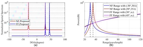
In the first set of experiments, the effectiveness of the MSNA in mixed source localization was analyzed. Suppose there are $K=4$ mixed sources, including $K_N=2$ near-field sources and $K_F=K-K_N=2$ far-field sources. The angles and distance parameters of the 2 near-field sources and 2 far-field sources are $\{{\theta }_1=-30°,r_1=30\lambda \}$, $\{{\theta }_2=30°,r_2=35\lambda \}$, $\{{\theta }_3=30°,r_3=\infty \}$, and $\{{\theta }_4=45°,r_4=\infty \}$, respectively. In the experiment, the SNR was set to 15 dB, and the snapshot number was $T=2000$. The simulation results are shown in Figure 2. In Figure 2a, a clear angular spectrum with four peaks can be observed, corresponding to the 2 near-field sources and 2 far-field sources in the mixed sources. In Figure 2b, within the Fresnel region, two distinct peaks corresponding to the two near-field sources can be observed, while the other two peaks from the far-field sources extend far beyond the Fresnel region. Thus, the proposed array structure and simulation algorithm can effectively achieve mixed source localization. Furthermore, the simulation results show that, when the azimuth angles of the near-field and far-field sources are identical, their azimuth angles and distances can still be accurately estimated.

Figure 2. Mixed source spatial spectrum under the MSNA. SNR = 15 dB and T = 2000 snapshots. (a) Angle spatial spectrum. (b) Distance spatial spectrum.

Experiment 2.

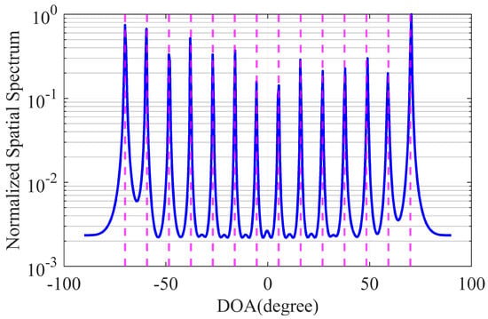
In the second set of experiments, we verified the underdetermined estimation capability of the proposed MSNA. We employed an MSNA with 13 sensors to perform mixed source localization for $K=14$ signals. The azimuth angles of the 14 sources were uniformly distributed between $[-70°,70°]$, including 7 NF sources and 7 FF sources. The ranges of these 14 signals were $\left\{30\lambda ,31\lambda ,32\lambda ,33\lambda ,34\lambda ,35\lambda ,36\lambda ,\infty ,\infty ,\infty ,\infty ,\infty ,\infty ,\infty \right\}$. In the experiment, the number of snapshots and the SNR were set to 30,000 and 15 dB, respectively. The simulation results are shown in Figure 3. From the simulation results, it can be observed that all 14 mixed-field sources were accurately estimated. Therefore, the underdetermined estimation capability of the MSNA was validated.

Figure 3. The ability to distinguish the number of signals.

Experiment 3.

In the third set of experiments, we compared the RMSE curves of the DOA estimation for five arrays. The mixed sources consisted of 3 near-field sources and 3 far-field sources, with angle and distance parameters $\{{\theta }_1=-60°,r_1=30\lambda \}$, $\{{\theta }_2=-45°,r_2=35\lambda \}$, $\{{\theta }_3=-15°,r_3=40\lambda \}$, $\{{\theta }_4=15°,r_4=\infty \}$, $\{{\theta }_5=45°,r_5=\infty \}$, $\{{\theta }_6=60°,r_6=\infty \}$:

1. 

RMSE versus SNR: As seen in the simulation results in Figure 4a, with a snapshot number of 3000 and an SNR ranging from −3 dB to 6 dB, the RMSE curves for all arrays follow the expected trend of decreasing as the SNR increases. From the simulation results, it is evident that the MSNA outperformed the other four array structures in DOA estimation performance across all SNRs.

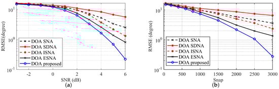Figure 4. RMSE of DOA estimates versus SNR and snapshots. (a) RMSE versus SNR. (b) RMSE versus snapshot.

2. 

RMSE versus snapshots: As shown in the simulation results in Figure 4b, with a fixed SNR of 15 dB and snapshots ranging from 50 to 3000, the RMSE curves for all arrays follow the expected trend of decreasing as the number of snapshots increases. It is evident from the simulation results that the MSNA outperformed the other four array structures in DOA estimation performance across all snapshot numbers.

Experiment 4.

In the fourth set of experiments, we compared the RMSE curves for distance estimation among five different arrays. The mixed sources consisted of four near-field sources and three far-field sources, with angle and distance parameters set as $\{{\theta }_1=-45°,r_1=29\lambda \}$, $\{{\theta }_2=-30°,r_2=32\lambda \}$, $\{{\theta }_3=-10°,r_3=35\lambda \}$, $\{{\theta }_4=30°,r_4=37\lambda \}$, $\{{\theta }_5=45°,r_5=\infty \}$, $\{{\theta }_6=60°,r_6=\infty \}$, and $\{{\theta }_7=70°,r_7=\infty \}$. As the distance of far-field signals tends to infinity, only near-field signals were considered when plotting the RMSE curves:

1. 

RMSE versus SNR: As shown in Figure 5a, with a snapshot number of 3000 and the SNR ranging from −3 dB to 15 dB, the RMSE curves for all arrays follow the expected trend of decreasing as the SNR increases. From the simulation results, it is evident that the MSNA consistently exhibited a lower RMSE across all SNR levels compared to the other four array structures. This indicates that the MSNA outperformed the other arrays in terms of distance estimation performance.

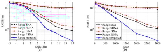Figure 5. RMSE of range estimates versus SNR and snapshots. (a) RMSE versus SNR. (b) RMSE versus snapshot.

2. 

RMSE versus snapshots: As depicted in Figure 5b, with the SNR set at 15 dB and snapshots ranging from 50 to 3000, the RMSE curves for all arrays exhibit the expected behavior of decreasing as the number of snapshots increases. From the simulation results, it is evident that the MSNA consistently demonstrated superior angle estimation performance compared to the other four arrays across all snapshot numbers.

Experiment 5.

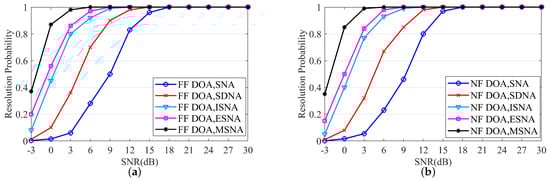
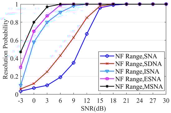
In the fifth set of experiments, we conducted a comparative analysis of the resolution performance probability of the proposed MSNA. The results are shown in Figure 6 and Figure 7. During the experiment, the number of snapshots was set to 1500, and the SNR ranged from [−3 dB, 30 dB]. In Figure 6, we compare the DOA estimation resolution performance for five different arrays structures. Figure 6a,b show the DOA estimation resolution for pure far-field sources and pure near-field sources, respectively. The parameters for the pure far-field sources were set to $\{{\theta }_1=10°,r_1=\infty \}$ and $\{{\theta }_2=13°,r_2=\infty \}$, while the parameters for the pure near-field sources were set to $\{{\theta }_3=10°,r_3=30\lambda \}$ and $\{{\theta }_4=13°,r_4=30\lambda \}$. In Figure 7, we compare the resolution performance of the range estimation for five different arrays. Since the range for far-field sources is infinite and cannot be used for resolution performance comparison, we selected a pure near-field scenario. The parameters for the two near-field sources were set to $\{{\theta }_5=45°,r_5=30\lambda \}$ and $\{{\theta }_6=45°,r_6=32\lambda \}$. The experimental results indicate that the proposed MSNA exhibits superior resolution performance compared to other array structures under the same conditions. Specifically, at a low SNR, the DOA and range resolution capabilities of the MSNA outperformed those of other arrays.

Figure 6. Probability curves of DOA estimation versus SNR. (a) Pure far-field sources. (b) Pure near-field sources.

Figure 7. Probability curves of range estimation versus SNR.

5. Conclusions

To address mixed source localization and enhance the underdetermined estimation capability of array structures, this paper introduces a Modified Symmetric Nested Array (MSNA) structure. Additionally, a mixed-source-estimation algorithm for the MSNA is designed using the subarray partition method and higher order cumulants. Compared to other arrays, the MSNA proposed in this paper has a larger array aperture, effectively enhancing the resolution; it also possesses a higher number of continuous lags, improving the array’s degrees of freedom and exhibiting better estimation performance in underdetermined estimations. The simulation results demonstrate that, for mixed source localization, under a constant SNR and snapshot conditions, the MSNA achieves higher estimation accuracy and resolution. Therefore, the performance of the proposed MSNA is superior to existing arrays in the scenario of mixed source localization.

References

- Zamani, H.; Zayyani, H.; Marvasti, F. An iterative dictionary learning-based algorithm for DOA estimation. IEEE Commun. Lett. 2016, 20, 1784–1787. [Google Scholar] [CrossRef]
- Liu, Y.; Liu, H.; Xia, X.-G.; Wang, L.; Bi, G. Target localization in multipath propagation environment using dictionary-based sparse representation. IEEE Access 2019, 7, 150583–150597. [Google Scholar] [CrossRef]
- Yue, Y.; Wang, Y.; Xing, F.; Shi, Z.; Liao, G. Polynomial rooting-based parameter estimation for polarimetric monostatic MIMO radar. Signal Process. 2023, 212, 15648–15664. [Google Scholar] [CrossRef]
- Yue, Y.; Zhou, C.; Xing, F.; Choo, K.-K.R.; Shi, Z. Adaptive beamforming for cascaded sparse diversely polarized planar array. IEEE Trans. Veh. Technol. 2023, 72, 3099. [Google Scholar] [CrossRef]
- Yue, Y.; Zhang, Z.; Shi, Z. Generalized Widely Linear Robust Adaptive Beamforming: A Sparse Reconstruction Perspective. IEEE Trans. Aerosp. Electron. Syst. 2024, 1–11. [Google Scholar] [CrossRef]
- Liu, Y.; Tan, Z.-W.; Khong, A.W.H.; Liu, H. Joint source localization and association through overcomplete representation under multipath propagation environment. In Proceedings of the ICASSP 2022-2022 IEEE International Conference on Acoustics, Speech and Signal Processing (ICASSP), Singapore, 23–27 May 2022. [Google Scholar]
- Liu, Y.; Liu, H. Target height measurement under complex multipath interferences without exact knowledge on the propagation environment. Remote Sens. 2022, 14, 3099. [Google Scholar] [CrossRef]
- Schmidt, R. Multiple emitter location and signal parameter estimation. IEEE Trans. Antennas Propag. 1986, 34, 276–280. [Google Scholar] [CrossRef]
- Roy, R.; Kailath, T. ESPRIT-estimation of signal parameters via rotational invariance techniques. IEEE Trans. Acoust. Speech Signal Process. 1989, 37, 984–995. [Google Scholar] [CrossRef]
- Starer, D.; Nehorai, A. Passive localization of near-field sources by path following. IEEE Trans. Signal Process. 1994, 42, 677–680. [Google Scholar] [CrossRef]
- Grosicki, E.; Abed-Meraim, K.; Hua, Y. A weighted linear prediction method for near-field source localization. IEEE Trans. Signal Process. 2005, 53, 3651–3660. [Google Scholar] [CrossRef]
- Du, W.; Kirlin, R.L. Improved spatial smoothing techniques for DOA estimation of coherent signals. IEEE Trans. Signal Process. 1991, 39, 1208–1210. [Google Scholar] [CrossRef]
- Lee, K. Deep learning-aided coherent direction-of-arrival estimation with the FTMR algorithm. IEEE Trans. Signal Process. 2022, 70, 1118–1130. [Google Scholar]
- Brandstein, M.; Ward, D. Microphone Arrays: Signal Processing Techniques and Applications; Springer Science & Business Media: Berlin/Heidelberg, Germany, 2001. [Google Scholar]
- Liang, J.; Liu, D. Passive localization of mixed near-field and far-field sources using two-stage MUSIC algorithm. IEEE Trans. Signal Process. 2009, 58, 108–120. [Google Scholar] [CrossRef]
- He, J.; Swamy, M.N.S.; Ahmad, M.O. Efficient application of MUSIC algorithm under the coexistence of far-field and near-field sources. IEEE Trans. Signal Process. 2011, 60, 2066–2070. [Google Scholar] [CrossRef]
- Liu, G.; Sun, X. Spatial differencing method for mixed far-field and near-field sources localization. IEEE Signal Process. Lett. 2014, 21, 1331–1335. [Google Scholar]
- Jiang, J.-j.; Duan, F.-j.; Wang, X.-q. An efficient classification method of mixed sources. IEEE Sens. J. 2016, 16, 3731–3734. [Google Scholar]
- Zuo, W.; Xin, J.; Zheng, N.; Sano, A. Subspace-based localization of far-field and near-field signals without eigendecomposition. IEEE Trans. Signal Process. 2018, 66, 4461–4476. [Google Scholar] [CrossRef]
- Yang, Y.; Shi, H.; Chen, J.; Wang, S. A Low Complexity Mixed Sources Localization Algorithm without Spectral Peak Search. In Proceedings of the 2023 5th International Conference on Intelligent Control, Measurement and Signal Processing (ICMSP), Chengdu, China, 19–21 May 2023; pp. 1118–1121. [Google Scholar]
- Zheng, Z.; Fu, M.; Wang, W.-Q.; Zhang, S.; Liao, Y. Localization of mixed near-field and far-field sources using symmetric double-nested arrays. IEEE Trans. Antennas Propag. 2019, 67, 7059–7070. [Google Scholar] [CrossRef]
- Tian, Y.; Lian, Q.; Xu, H. Mixed near-field and far-field source localization utilizing symmetric nested array. Digit. Signal Process. 2018, 73, 16–23. [Google Scholar] [CrossRef]
- Wang, B.; Liu, J.; Sun, X. Mixed sources localization based on sparse signal reconstruction. IEEE Signal Process. Lett. 2012, 19, 487–490. [Google Scholar] [CrossRef]
- Ebrahimi, A.A.; Abutalebi, H.R.; Karimi, M. Localisation of mixed near-field and far-field sources using the largest aperture sparse linear array. IET Signal Process. 2018, 12, 155–162. [Google Scholar] [CrossRef]
- Wang, Y.; Cui, W.-J.; Du, Y.; Ba, B. A novel sparse array for localization of mixed near-field and far-field sources. Int. J. Antennas Propag. 2021, 2021, 3960361. [Google Scholar] [CrossRef]
- Shen, Q.; Liu, W.; Cui, W.; Wu, S.; Pal, P. Simplified and enhanced multiple level nested arrays exploiting high-order difference co-arrays. IEEE Trans. Signal Process. 2019, 67, 3502–3515. [Google Scholar] [CrossRef]
- Rajamäki, R.; Koivunen, V. Sparse symmetric linear arrays with low redundancy and a contiguous sum co-array. IEEE Trans. Signal Process. 2021, 69, 1697–1712. [Google Scholar] [CrossRef]
- Shi, J.; Wen, F.; Liu, Y.; Liu, Z.; Hu, P. Enhanced and generalized coprime array for direction of arrival estimation. IEEE Trans. Aerosp. Electron. Syst. 2022, 59, 1327–1337. [Google Scholar] [CrossRef]
- Pal, P.; Vaidyanathan, P.P. Nested arrays: A novel approach to array processing with enhanced degrees of freedom. IEEE Trans. Signal Process. 2010, 58, 4167–4181. [Google Scholar] [CrossRef]
- Vaidyanathan, P.P.; Pal, P. Sparse sensing with co-prime samplers and arrays. IEEE Trans. Signal Process. 2010, 59, 573–586. [Google Scholar] [CrossRef]
- Zhou, C.; Gu, Y.; Shi, Z.; Haardt, M. Structured Nyquist correlation reconstruction for DOA estimation with sparse arrays. IEEE Trans. Signal Process. 2023, 71, 1849–1862. [Google Scholar] [CrossRef]
- Zheng, H.; Zhou, C.; Shi, Z.; Gu, Y.; Zhang, Y.D. Coarray tensor direction-of-arrival estimation. IEEE Trans. Signal Process. 2023, 71, 1128–1142. [Google Scholar] [CrossRef]
Disclaimer/Publisher’s Note: The statements, opinions and data contained in all publications are solely those of the individual author(s) and contributor(s) and not of MDPI and/or the editor(s). MDPI and/or the editor(s) disclaim responsibility for any injury to people or property resulting from any ideas, methods, instructions or products referred to in the content. |
© 2024 by the authors. Licensee MDPI, Basel, Switzerland. This article is an open access article distributed under the terms and conditions of the Creative Commons Attribution (CC BY) license (https://creativecommons.org/licenses/by/4.0/).