Article

Tree Canopy Volume Extraction Fusing ALS and TLS Based on Improved PointNeXt

1
College of Information Science and Technology & College of Artificial Intelligence, Nanjing Forestry University, Nanjing 210037, China
2
Institute of Forest Resource Information Techniques, Chinese Academy of Forestry, Beijing 100091, China
3
College of Forestry, Hebei Agricultural University, Baoding 071051, China
*
Author to whom correspondence should be addressed.
Remote Sens. 2024, 16(14), 2641; https://doi.org/10.3390/rs16142641
Submission received: 6 June 2024 / Revised: 10 July 2024 / Accepted: 17 July 2024 / Published: 19 July 2024

Abstract

:
Canopy volume is a crucial biological parameter for assessing tree growth, accurately estimating forest Above-Ground Biomass (AGB), and evaluating ecosystem stability. Airborne Laser Scanning (ALS) and Terrestrial Laser Scanning (TLS) are advanced precision mapping technologies that capture highly accurate point clouds for forest digitization studies. Despite advances in calculating canopy volume, challenges remain in accurately extracting the canopy and removing gaps. This study proposes a canopy volume extraction method based on an improved PointNeXt model, fusing ALS and TLS point cloud data. In this work, improved PointNeXt is first utilized to extract the canopy, enhancing extraction accuracy and mitigating under-segmentation and over-segmentation issues. To effectively calculate canopy volume, the canopy is divided into multiple levels, each projected into the xOy plane. Then, an improved Mean Shift algorithm, combined with KdTree, is employed to remove gaps and obtain parts of the real canopy. Subsequently, a convex hull algorithm is utilized to calculate the area of each part, and the sum of the areas of all parts multiplied by their heights yields the canopy volume. The proposed method’s performance is tested on a dataset comprising poplar, willow, and cherry trees. As a result, the improved PointNeXt model achieves a mean intersection over union (mIoU) of 98.19% on the test set, outperforming the original PointNeXt by 1%. Regarding canopy volume, the algorithm’s Root Mean Square Error (RMSE) is 0.18 m3, and a high correlation is observed between predicted canopy volumes, with an R-Square (R2) value of 0.92. Therefore, the proposed method effectively and efficiently acquires canopy volume, providing a stable and accurate technical reference for forest biomass statistics.

1. Introduction

The canopy serves as a crucial component of a tree, providing the essential material foundation for its growth and development [1,2]. The canopy consists of a mass of branches and leaves growing outwards from the trunk, playing an important role in photosynthesis, carbon dioxide absorption, and soil and water conservation [3,4,5]. The dimensions of the canopy are intricately linked to tree growth and serve as indicators of overall tree health [6], making them important parameters in forest metrology. In addition to canopy width and canopy height, canopy volume stands as a fundamental descriptor of a tree canopy. Within the biomass calculation process [7,8], incorporating canopy volume enhances the fitting accuracy of the Above-Ground Biomass (AGB) model, thereby establishing a robust foundation for crafting a more precise AGB model [9,10]. Depending on the methods of data collection, canopy volume calculation methods can be broadly categorized into traditional techniques and remote sensing (RS) methods.
Traditional volumetric measurements are inaccurate, costly, and time-consuming. With the development of RS technology, more detailed tree data can be collected, making canopy volume measurements more effective. Calculating canopy volumes using RS images and LiDAR point clouds has garnered significant attention in recent years. Some methods have been proposed to extract canopy volumes. Previous studies have extracted canopy volume from ALS data using the 3D convex hull technique [11]. Yan et al. [12] proposed a concave hull method for calculating the canopy volume of a single tree based on vehicle-mounted LiDAR data. However, the above method does not take into account gaps in the tree canopy, which can affect the results of canopy volume calculation. Ross et al. [13] used voxel optimization for estimating the voids present in the canopy. The method is limited to the fact that the size of the voxel has a significant impact on the calculation of the canopy volume. In addition, different RS data choices (including 2D imagery, multispectral and hyperspectral imagery, and ground-based and UAV LIDAR data, among others) can affect the calculation of canopy volume [14]. Multispectral or hyperspectral images are used to calculate canopy volume [15,16]. However, the lack of 3D information and canopy structure description in 2D images can limit the accuracy of canopy volume calculations. TLS point cloud data can accurately provide the 3D coordinates and spatial resolution of the canopy, which can be used to calculate the canopy volume [17]. However, occlusion occurs in complex trees, resulting in incomplete capture of the canopy’s morphology. ALS point clouds also have high-resolution data that can be used to calculate canopy volume [18]. However, this is limited by issues such as flight altitude and upper canopy occlusion, and cannot meet the requirements for the accurate estimation of canopy volume. Therefore, fusing TLS and ALS data can mitigate the individual limitations of these sources, providing comprehensive canopy information. TLS can provide a more detailed description of the canopy structure, while ALS can provide extensive coverage and height information. By fusing these two data sources, canopy data with both extensive coverage and high resolution can be obtained, allowing for the accurate estimation of canopy volumes.
With the development of deep learning, point cloud segmentation networks have become widely used. The classic PointNet, known for its few parameters, is highly regarded among scholars [19]. However, a drawback of PointNet is its inability to capture local features of the point cloud. Even when points are mapped to a higher-dimensional space, it still loses significant feature information of the local points. Despite this limitation, PointNet generally performs well in scene segmentation. Subsequently, researchers introduced PointNet++ [20], the first model capable of extracting information from local points as features. In this paper, to enhance the accuracy of canopy volume calculation, we utilize a deep learning semantic segmentation network to extract the canopy volume. Researchers have proposed some deep learning networks for segmentation. For instance, He et al. [21] proposed a parallel fusion neural network that considers both local and global semantic information for citrus tree canopy segmentation. Martins et al. [22] proposed a region-based CNN object instance segmentation algorithm for the semantic segmentation of tree canopies in urban environments using aerial RGB imagery. Additionally, Zhang et al. [23] proposed an adaptive segmentation method based on extreme offset deep learning. They designed an individual tree segmentation (ITS) set aggregation strategy based on the gradient change criterion to address over-segmentation generated by random offsets, achieving precise ITS. Xu and Wang [24] introduced a new method of extracting street trees by dimensional feature analysis and an improved FCM method. Kim et al. [25] proposed a new approach utilizing the PointNet++ model for segmenting the canopy, trunk, and branches of trees. Hu et al. [26] presented a study on point cloud segmentation, combining improved point converters and individual trees for hierarchical clustering, aimed at fine-grained segmentation. The recent PointNeXt network model [27] recognizes the performance potential of PointNet++. The improved performance of networks such as Point Transformer are mainly due to better data augmentation, optimization methods, and larger models [28]. PointNeXt achieves an increase in overall model performance through improved training strategies and model scaling. Through the continuous research of the above scholars, the use of 3D point cloud data to solve practical problems has gradually taken over the dominant position. The above model lays a very important foundation for the improvement of the canopy segmentation network in this paper, which utilizes the improved semantic segmentation of PointNeXt to achieve accurate segmentation and provide precise point cloud data for the calculation of canopy volumes.
Though much research has been done on canopy volume, there are still some problems, such as the following: (1) The selection of datasets can influence canopy volume calculations. (2) Under-segmentation or over-segmentation affects the completeness of canopy extraction. (3) Gaps in the canopy can affect the accuracy of canopy volume calculations. To tackle these problems, this paper proposes canopy volume extraction based on an improved PointNeXt model, fusing ALS and TLS point cloud data to achieve accurate canopy segmentation and volume calculation.
The main contributions of this paper are as follows: (1) PointNeXt is improved using Grouped Vector Attention (GVA) and Edge Convolution (Edgeconv), thus realizing the segmentation of the tree canopy and trunk and providing the basis for subsequent canopy volume calculation. (2) Registration is performed to fuse ALS and TLS data. (3) Due to the complexity of point cloud data computation, incorporating KdTree accelerates point cloud searches, thereby speeding up hierarchical clustering processes. (4) The improved Mean Shift algorithm uses a combination of point cloud position information ( x , y , z ) and color information ( r , g , b ) . The convex hull algorithm for hierarchical clustering combined with KdTree is proposed to realize the accurate calculation of canopy volume. (5) The effectiveness of the algorithm is verified by a series of experiments.

2. Materials

2.1. Study Area

The data used in this study were mainly obtained from the Baima Campus of Nanjing Forestry University (31°61′N, 119°18′E). Data from Hung-tse Lake wetland (33°06′–33°40′N, 118°10′–118°52′E) were used as a reference for the validation experiments. Data collections took place in May, August, and November 2023, respectively. The geographical location is shown in Figure 1.

2.2. Data Acquisition

A 3D laser scanner, Trimble TX7 Laser Scanning, was used in data acquisition, and the detailed performance and indices are presented in Table 1. Using the Baima campus as the main study area, we selected 150 representative sample trees of different species (poplar, willow, and cherry) as the data source. To ensure the regional diversity of the data, 80 trees from the Hung-tse Lake wetland were also selected as validation data in this paper. In order to reduce computational errors, the data in this paper were collected under sunny and breezy conditions and mainly straight sample trees were selected. A summary of the field inventory data for the plots used for validation is presented in Table 2.
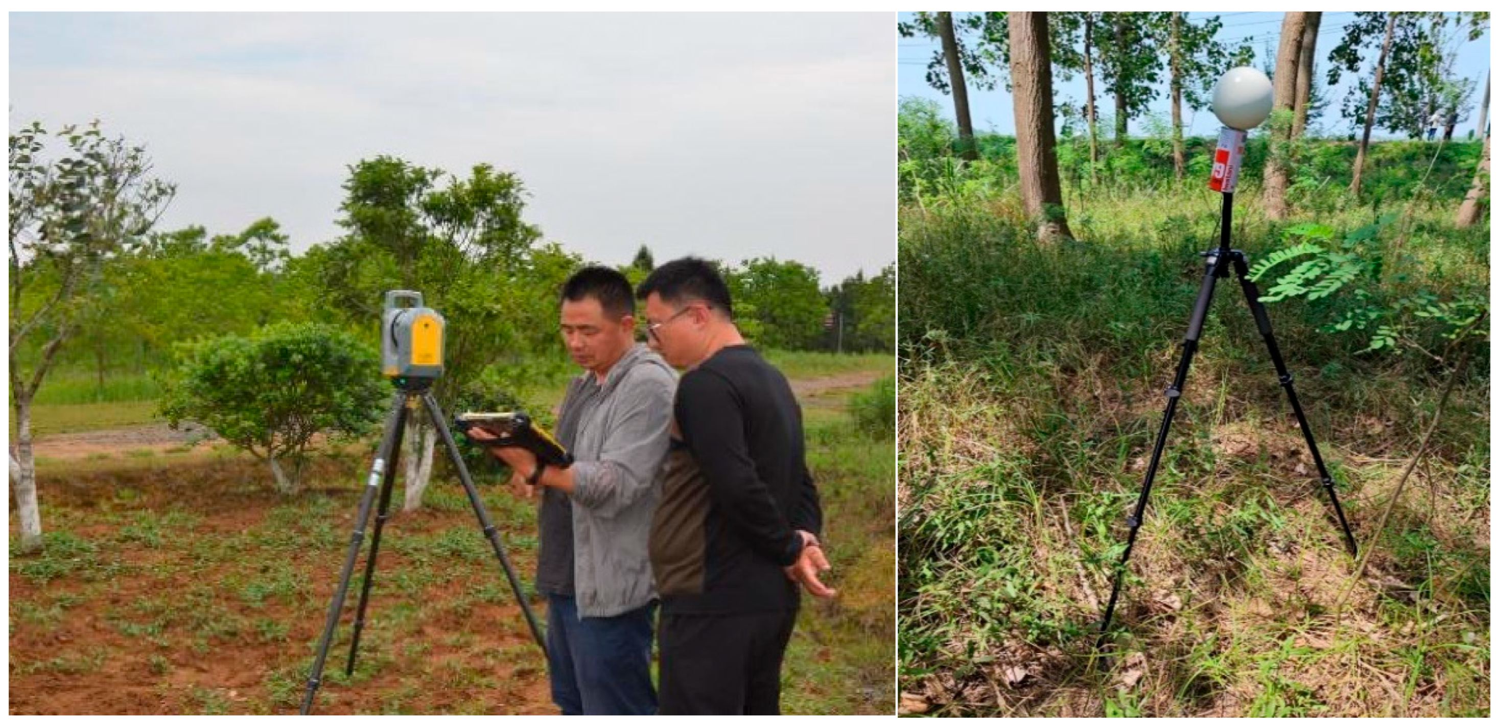
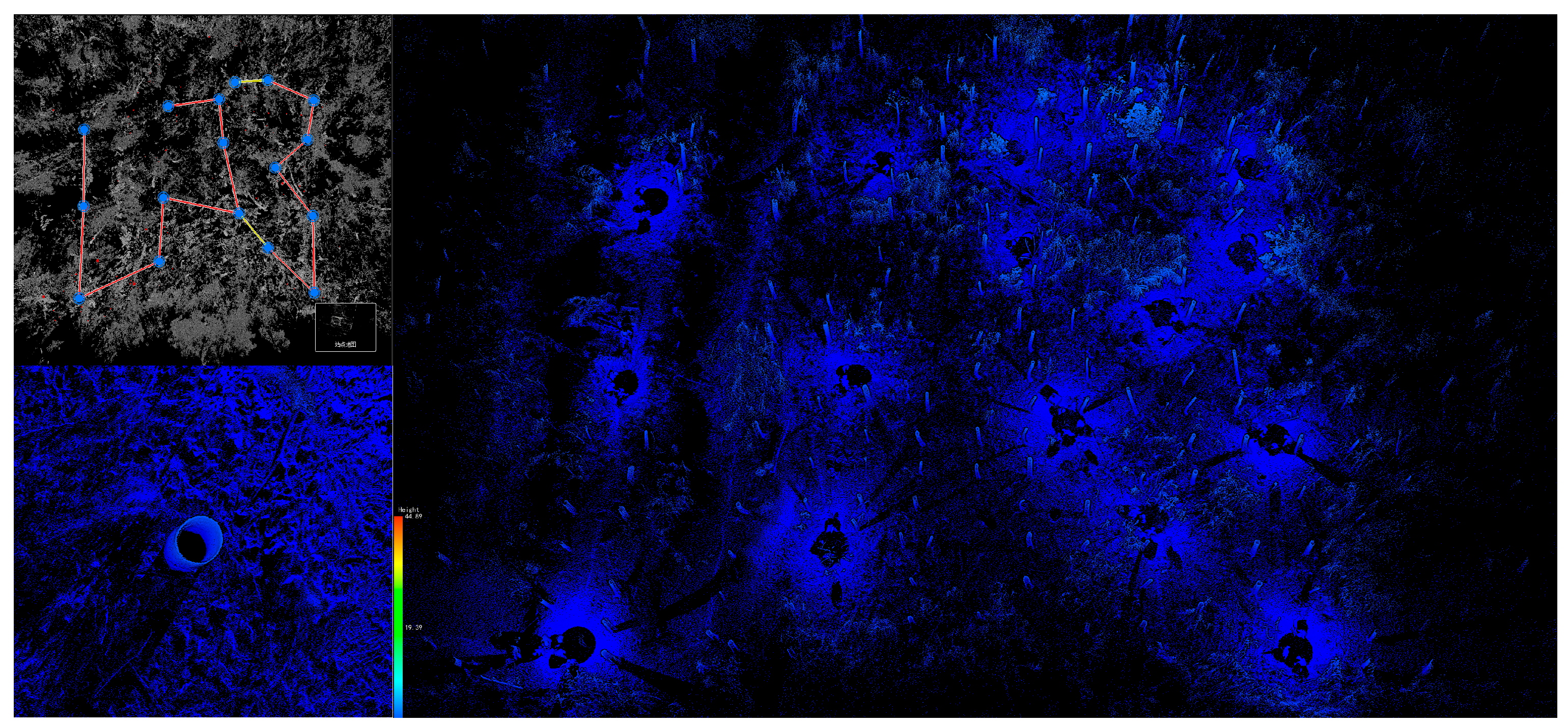
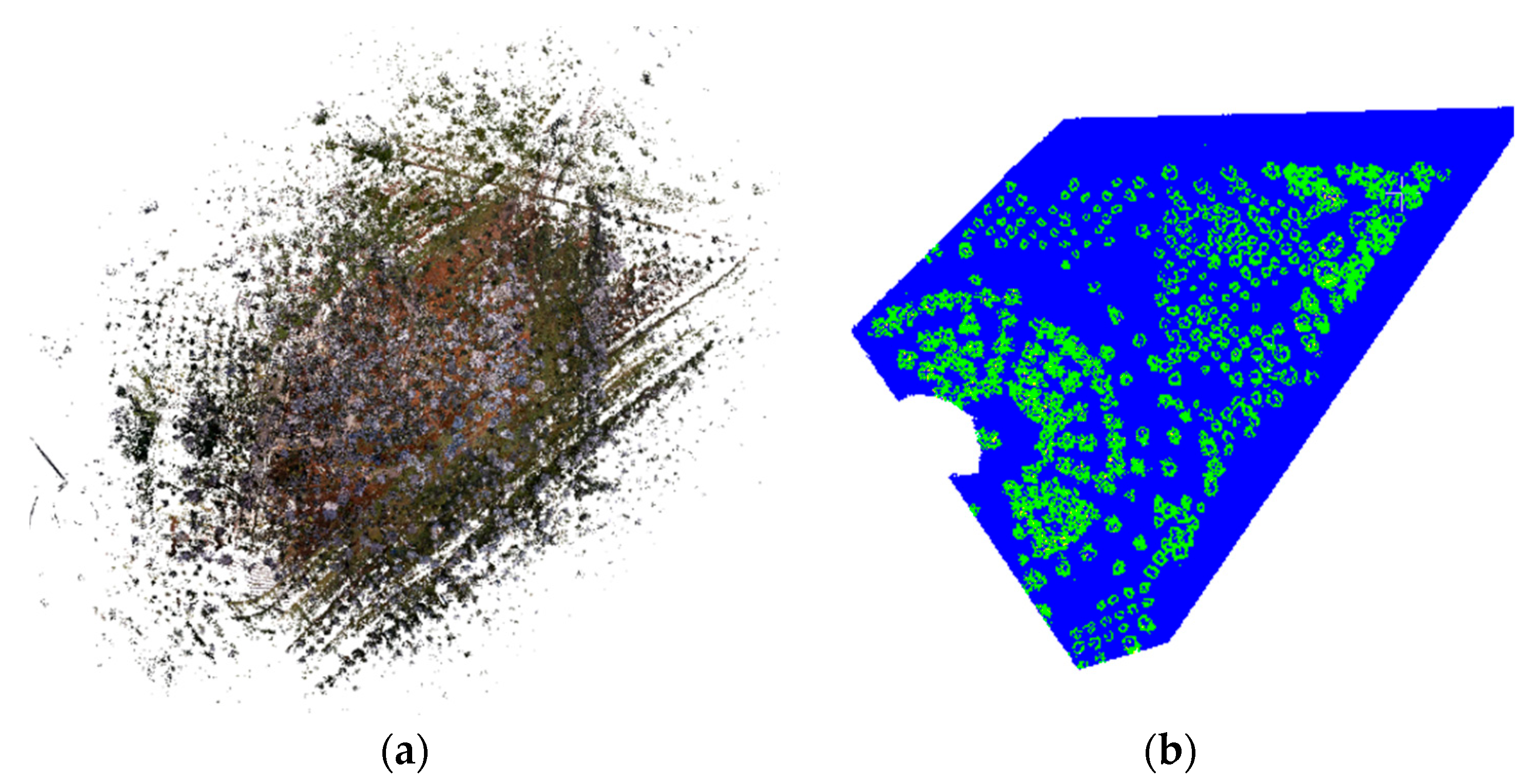
Our field measurement setup is shown in Figure 2. Multi-site scanning avoids the disadvantage of trees occluding each other, as occurs in the single-site scanning method [29]. In order to obtain accurate and comprehensive unobstructed TLS point cloud data of all trees, we used a multi-site scanning method for all the relevant tree point cloud data, and the distribution of the sites is shown in Figure 3. The initial TLS and ALS point cloud data are shown in Figure 4.

3. Methods

3.1. Framework of the Method

In this paper, the improved PointNeXt semantic segmentation network is used to extract tree canopy data. Then, the KdTree-based Hierarchical Clustering Projection Convex hull algorithm is used to calculate canopy volume.
The whole process is shown in Figure 5. Firstly, ALS and TLS registration obtain the complete point cloud dataset. Non-trees (including soil, weeds, etc.) are then removed from the point cloud data [26]. Next, the canopy is segmented using the improved PointNeXt network to obtain the canopy and trunk portions of each tree. Subsequently, the point cloud is stratified by a certain height h and the point cloud is searched quickly using KdTree to speed up the clustering. The area of each cluster is calculated by convex hull calculation and multiplied by h to obtain the volume of each class. Finally, all class volumes are summed to obtain the canopy volume.

3.2. Data Registration

The CloudCompare software (Version: 2.12.4), matched with a 3D laser scanner, was used to register the TLS and ALS point cloud data. Firstly, data from the same position is registered from each small incision section of the TLS and ALS point clouds. The ICP algorithm is used to find the rotation matrix, which has an RMSE of 0.18 m (calculated over 50,000 points). Then, the rotation matrix is used to register the TLS and ALS data as a whole, and finally the point cloud data with the complete structure is obtained. The registration process is shown in Figure 6.

3.3. Point Cloud Preprocessing

(1)
Filtering and denoising
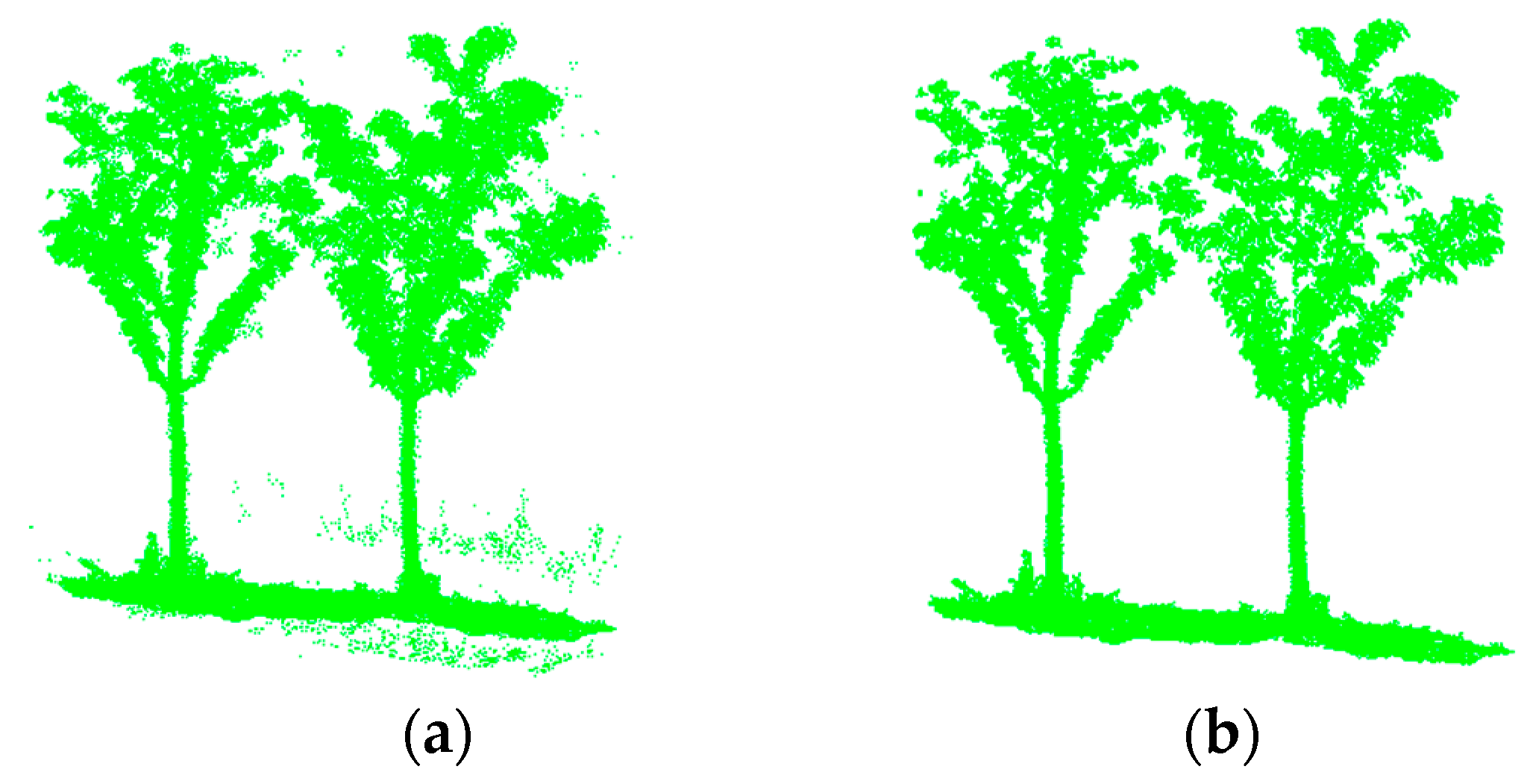
Laser scanners can capture large amounts of point cloud data from real trees, but noise points caused by environmental factors can have a significant impact on point cloud quality. Therefore, it is very important to filter and denoise the point cloud. To remove these noise points, it is necessary to inspect and remove extraneous point clouds that are several meters away from the point cloud tree. The point cloud filtering module Statistical Outlier Removal (SOR) in the Point Cloud Library was used in this study. This filtering is used to remove outlier noise points by setting two parameters, namely the neighbor point n and standard deviation threshold factor k, where n = 12, k = 1.0. An original point cloud and the filtered point cloud are shown in Figure 7.
(2)
Non-tree removal
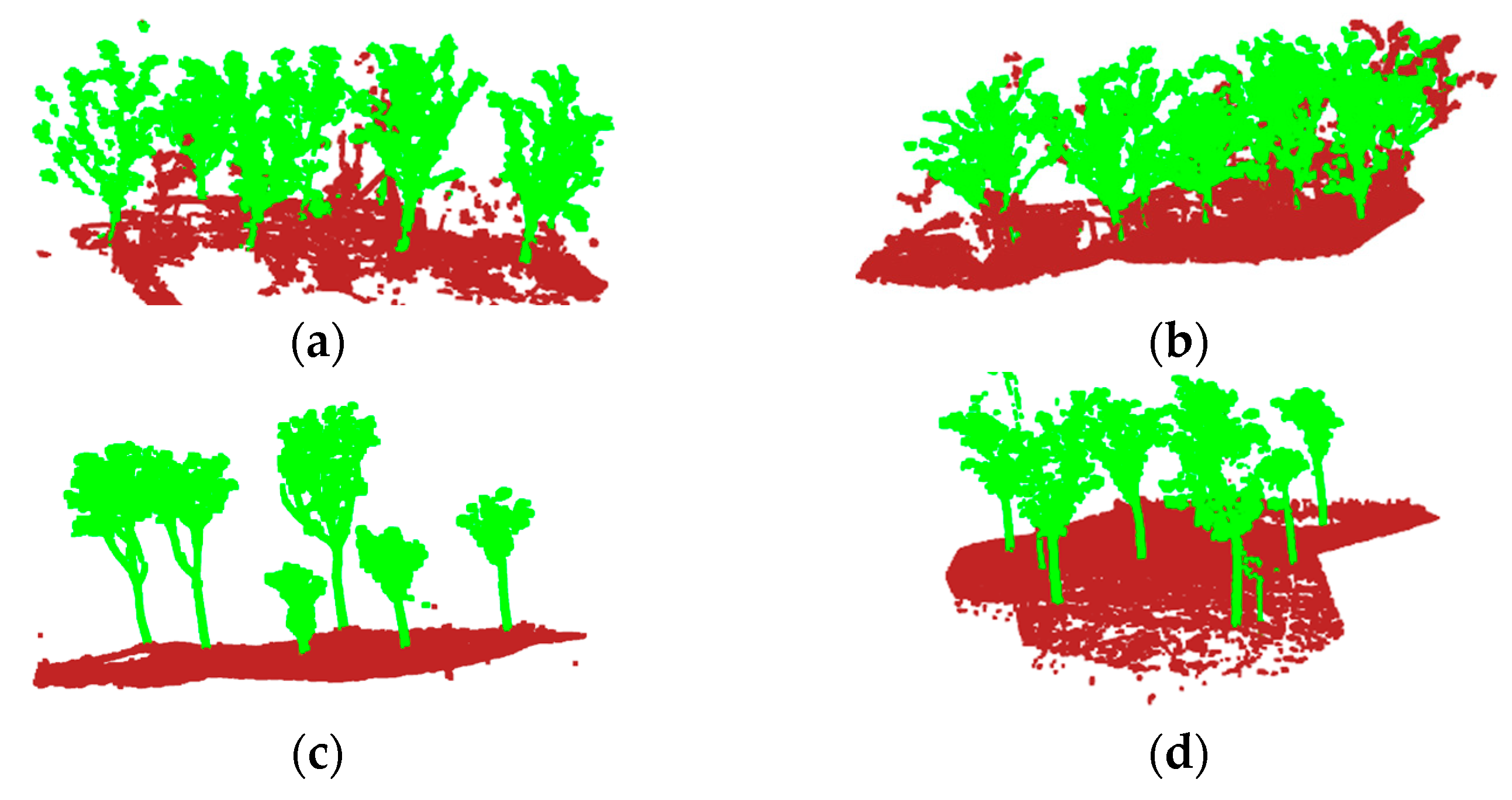
In this study, the point cloud data used contained non-tree data such as soil and weeds, which could not be removed using traditional filtering methods. However, manual removal of this data is also laborious, so the tree portion was finely segmented using a hierarchical clustering method [26]. The segmentation results are shown in Figure 8.

3.4. Extraction of Canopy: Division of Canopy and Trunk

In the point cloud data of this study, over-segmentation and under-segmentation occurs at the location of the intersection of the trunk and canopy using the classical deep learning network, which cannot be accurately judged, as shown in Figure 9.
Therefore, an improved novel semantic segmentation network is proposed to achieve accurate segmentation to improve canopy extraction accuracy in this paper.
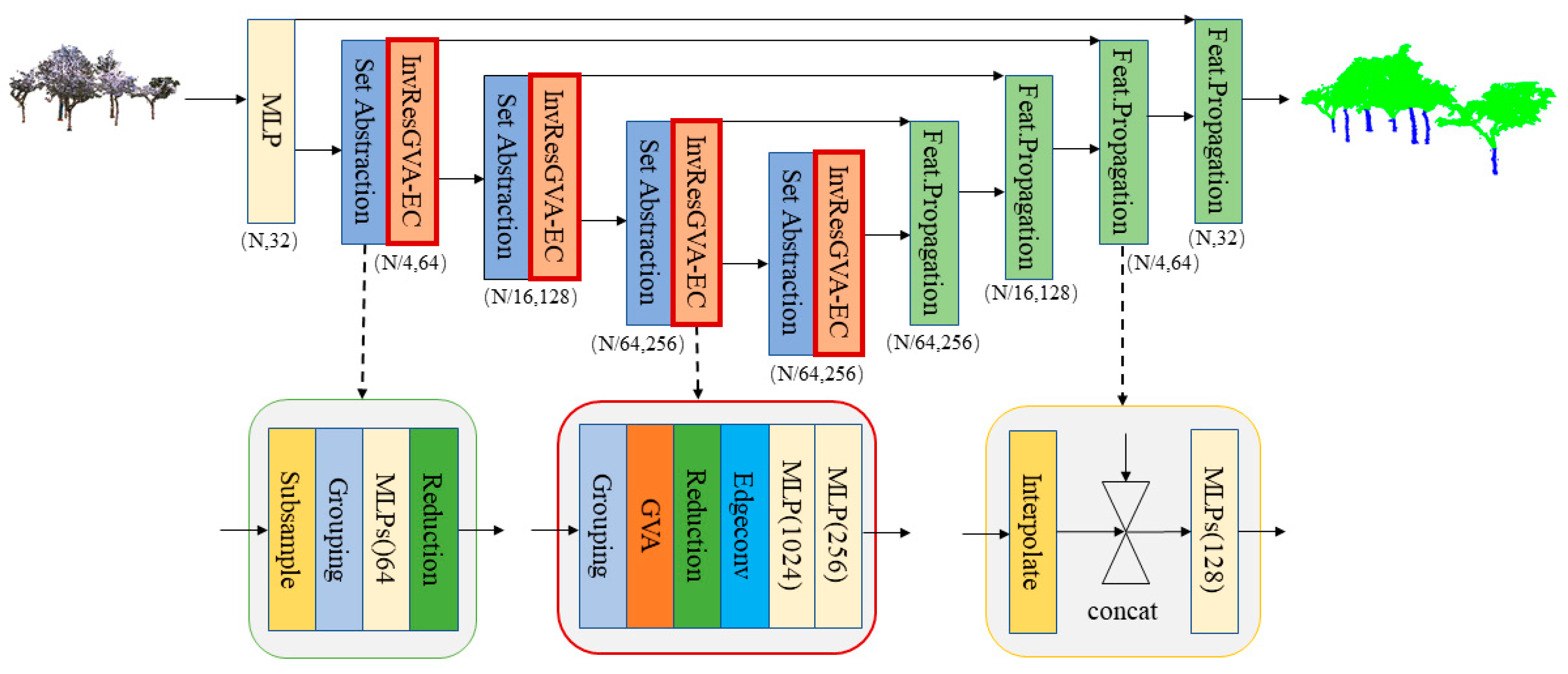
In the improved PointNeXt network, the original InvResMLP module is replaced by the new Inverted Residual Grouped vector attention (InvResGVA-EC) [30] block instead. Specifically, the first MLP layer in the InvResMLP module is replaced by Grouped vector attention, and the edge convolution (EdgeConv) [31] is embedded between the reduction layer and the second MLP layer. The overall network structure of the improved PointNeXt model is shown in Figure 10.
The blocks in the down-sampling process contain the SA module and InvResGVA-EC components, and the up-sampling process is mainly the Feature Propagation block. The SA module consists of Furthest Point Sampling (FPS), the grouping algorithm, and a set of MLPs and MaxPools, which down-sample, query the domain points, and perform local feature extraction and aggregation, respectively, for each point in the point cloud.
The PointNeXt network features the Inverted Residual MLP (InvResMLP) block. The InvResMLP module has a residual module added between the inputs and outputs to alleviate the problem of vanishing gradients. There are three layers of MLPs in it; the first layer of the MLP implementation acts on the domain features and is located between the grouping and reduction layers. The purpose is to reduce the feature dimension while retaining the local information, but it is not possible to continue learning on the retained local feature point cloud. Therefore, this paper proposes to replace the first layer of MLP with grouping vector attention (GVA), which can re-learn the local information and extract more refined features.
Currently, the prevailing trend is to extract local information through the use of self-attention. For point cloud information processing, this is mainly the feature extraction of points. The improved network structure in this paper introduces grouped vector attention, which divides vectors into small pieces and computes each piece independently. Compared with ordinary vector attention, this can reduce the computational complexity compared to ordinary vector attention and, at the same time, it can improve the ability to identify local point cloud features, which is not available in the first layer of MLPs.
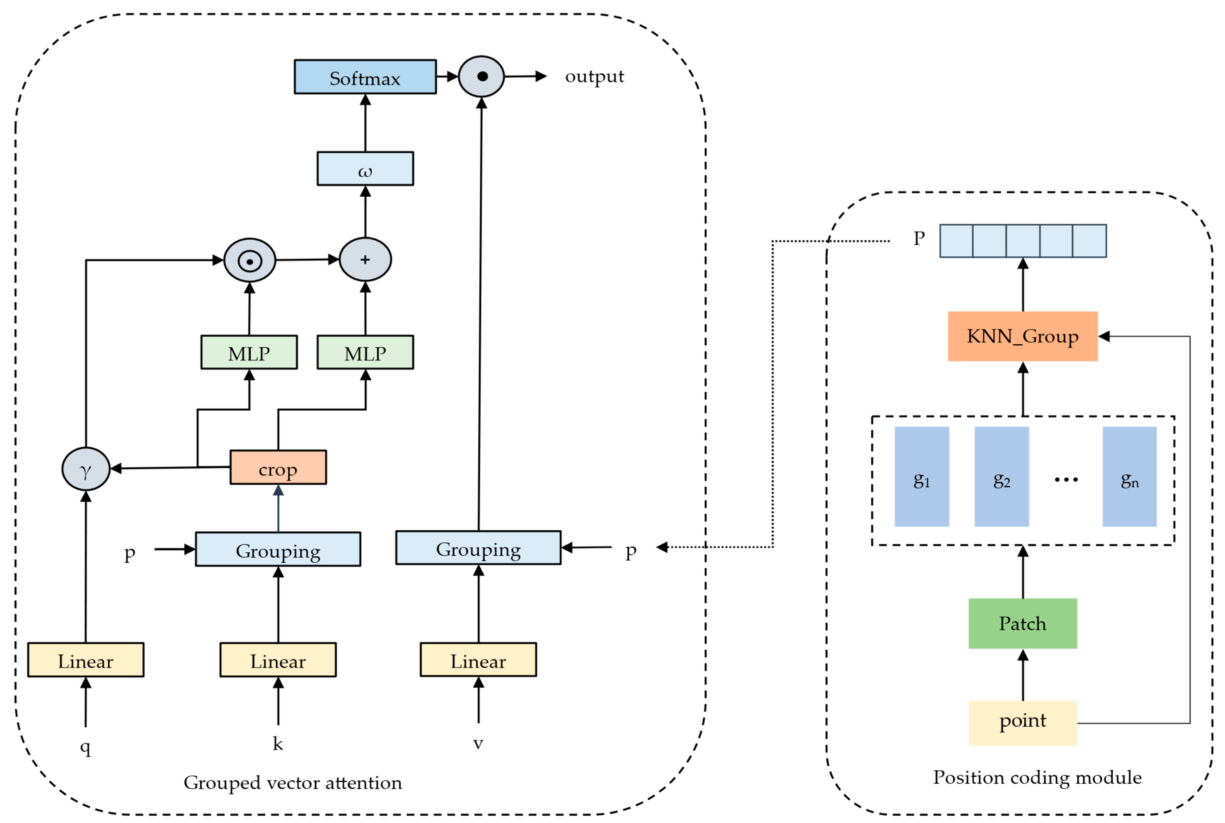
Grouped vector attention (GVA):   M = P , F is a 3D point cloud containing a set of points x i = ( p i , f i ) M , where p i R 3 denotes the position of the point and f i R c denotes the features of the point. Each point x i is used to predict a class label. Groupable vector attention is described as follows:
The GVA module divides the channels v R c equally into g groups 1 g c ) . The output of its weight coding layer has g channels, and the channels v of the same attention group share the same weight of the grouped attention vectors. The specific block structure is shown in Figure 11 below.
The position encoding function can improve the ability of attention feature extraction. In this paper, we use parametric position coding, as shown in Figure 11. Firstly, the 3D point cloud data are grouped by offset data statistics to obtain the result offset, and then combined with the point cloud information, grouped by KNN to obtain the mapping coding information, and the position coding information P is obtained.
The specific mathematical formulae are as follows:
w i j = ω ( γ ( q i , k i ) )
f i a t t n = x j M ( p i ) l = 1 g m = 1 c g S o f t m a x ( W i ) j l v j l c g + m
where γ is the relation function (the minus sign is used here) and ω : R C R g defines the learnable grouping weight encoding for the next section. The mathematical formula for number (2) is grouped vector aggregation.
The encoding functions for the relation vector, weight vector, and value vector are illustrated in Figure 12.
We group the vectors, and after grouping we can solve the problem that the parameters of the weight coding layer increase with the depth of the network and the number of feature coding channels, which in turn improves the efficiency and generalization of the model. The schematic comparison before and after grouping is shown in Figure 12.
Each square represents a scalar and each row of them represents a vector. A feature dimension of 4 is assumed for the above block. Different colored lines represent different operations. The orange line is used for the input relational scalar and the blue line marks which feature is affected by the weight of the input scalar.
The pseudo-code for the specific implementation process of GVA is shown below:
Input: feat, coord, offset #features, point cloud coordinates, offset
Output: feat
1.     procedure forward (feat, coord, offset)
2.      P = Knn_group(neighbour, coord, offset)
3.      query =Linear_q(feat)
4.      key = Linear_k(feat)
5.      value = Linear_v(feat)
6.      key = pointops.grouping(P, key, coord)
7.      value = pointops.grouping(P, value, coord)
8.      pos = key[:, :, 0:3]
9.      key = key[:, :, 3:]
10.      relation_qk = key-query.unsqueeze(1) #unsqueeze: add one to the second dimension of the query
11.      weight = weight_encoding(relation_qk)
12.      weight = Softmax(weight)
13.      weight = attention_drop(weight)
14.      mask = Sign(reference_index + 1)
15.      weight = Einsum(weight, mask) #dimensionality transformation: “n s g, n s -> n s g”
16.      feat = Einsum(value, weight) #dimensionality transformation: “n s g i, n s g -> n g i-> n (g i)”
17.      return feat
18.    end procedure
The meaning of the offset in the pseudo-code is as follows: Suppose the number of the batch is 4 and the number of points in the four samples are n1, n2, n3, and n4. Then, the offset is [n1, n1+ n2, n1+ n2+ n3, n1+ n2+ n3+ n4]. The obtained coordinate size is torch. Size([n1+ n2+ n3+ n4, 3]).
The second MLP layer of InvResMLP is not able to achieve keeping dynamic follow up on the local features of the point cloud. In this paper, inspired by DGCNN, we improve the InvResMLP module by embedding an edge convolution (EdgeConv) between the reduction layer and the second MLP layer.
DGCNN exploits local geometric structures by constructing a local neighborhood graph and applying convolution-like operations on edges connecting adjacent pairs of points. The core design uses edge convolution (EdgeConv). EdgeConv has the property of being an intermediate between translation invariance and nonlocalization, i.e., not only can it maintain alignment invariance, but it can also capture local geometric features. Unlike graph convolution, the graph of DGCNN is not fixed and is dynamically followed after each layer of the network. The network module design of EdgeConv is shown in Figure 13.
The EdgeConv principle is introduced, and the computational principle is shown in Figure 14.
Assume a D-dimensional point cloud with n points, defined as X = x 1 , x n R D . Later layers receive the output of the previous layer in a deep neural network, and the dimension D can also denote the feature dimension of a particular layer. The local structure of the point cloud is represented by building a graph of the k-nn. The nearest point x j i 1 , , x j i k to x i contains many directed edges i , j i 1 , , i , j i k .
We define the edge features as follows:
e i j = h Θ ( x i , x j x i )
where h Θ : R D × R D R D ' utilizes a nonlinear function comprising learnable parameters denoted as Θ . This paper employs the asymmetric edge function, effectively amalgamating global shape features.
Moreover, the EdgeConv operation is augmented by applying a symmetric aggregation operation to all pertinent edge features originating from each vertex. Mathematically, the formula can be expressed as follows:
x i = j : ( i , j ) ε h Θ ( x i , x j x i )  
where x i serves as the center point and x j : ( i ,   j ) ε serves as its surrounding patches.
This paper focuses on proposing an improved PointNeXt model which mainly modifies and replaces the InvResMLP module and replaces the MLP of the first layer with the use of GVA to improve the ability of recognizing local point clouds. Meanwhile, EdgeConv is added between the reduction layer and the second MLP layer to achieve the fusion of global and local features and improve the segmentation effect.

3.5. Improved KdTree-Based Mean Shift Clustering of Point Cloud

In this paper, we enhance the efficiency of the Mean Shift clustering by implementing a KdTree, which optimizes the search process for point cloud data. At the same time, we improve Mean Shift to compute canopy volume more accurately. The implementation process is as follows:
(1)
Create KdTree
KdTree (K-Dimensional Tree) is a data structure that can be used to efficiently search for data points in a multidimensional space. In point cloud processing, the use of KdTree usually speeds up the process of searching and neighborhood querying, thus improving the efficiency of the algorithm [32,33].
(2)
Improved Mean Shift
In this study, we take the classical Mean Shift density clustering as the basis [34,35], and make the point cloud clustering effect more stable by introducing a new kernel function adapted to 3D point cloud data (combining the positional coordinates of the point cloud and RGB information). Assuming that there are two X i and X j , their coordinates are ( x i , y i , z i ) and ( x j , y j , z j ) , and their colors are ( r i , g i , b i ) and r j , g j , b j , the kernel function can be defined as follows:
K X i , X j = αe xp X i X j 2 2 σ 1 2 + βexp C i C j 2 2 σ 2 2
where X i X j denotes the Euclidean distance between spatial coordinates; C i C j denotes the Euclidean distance between color vectors. α and β are used as weighting coefficients to balance the coordinate information and color information. σ 1 and σ 2 are used as the bandwidth parameters of the Gaussian kernel which control the rate of similarity decay.

3.6. Calculating Canopy Volume

With the support of LiDAR point cloud data, canopy volume calculations have made great strides in using preprocessed canopy point cloud data for hierarchical projections. In this paper, we mainly process the tree canopy gaps to get the closest true volume of the tree canopy, using previously split tree canopy data before starting the calculation.
The method used in this paper is “Hierarch Point Cloud Layer Projection Clustering Convex Hull”, abbreviated as HPCP-CC. The whole process of the specific realization of tree canopy volume calculation is as follows:
Input: Canopy point cloud data P
Output: Canopy volume V
1.     procedure processPointCloud (P)
2.       pointCloud = load_and_sort_point_cloud (P)
3.       sliceHeight = 0.2 #Stratify the canopy point cloud data into layers
4.       layers = stratifyPointCloud (P, sliceHeight)
5.       for each layer in layers do
6.         project(layer) #Project point cloud for each layer in the xOy plane
7.        α = 0.8 #Clustering using improved KdTree-based Mean Shift
8.        β = 0.2
9.        σ 1 = 0.2
10.        σ 2 = 0.3
11.       for each layer in layers do
12.       KdTree = buildKdTree (layer)
13.       clusters = meanShiftClustering (layer, KdTree, α , β , σ 1 , σ 2 )
14.       for each cluster in clusters do
15.       area = calculateClusterArea(cluster) #Calculate the area of each cluster using the Graham scan method
16.       totalArea += area
17.       volume = 0
18.       for each layer in layers do #Calculate the volume of each layer
19.       layerVolume = calculateLayerVolume (totalArea, sliceHeight)
20.       V = V + layerVolume
21.       return V
22.    end procedure

3.7. Comprehensive Evaluation

(1)
Semantic segmentation network evaluation
The performance of the semantic segmentation model in this study is evaluated by the mean intersection over union (mIoU). The mIoU calculates the average of the IoU for each class, which is obtained by measuring the intersection and concatenation ratios between true and predicted. The scoring metrics are calculated as follows:
m I o U = 1 C i = 1 C p i i j = 1 C p i j + j = 1 C p j i p i i
where C is the category and P i j is the number of objects or points belonging to the i category but expected to belong to the j category.
(2)
Volumetric modeling accuracy assessment
The accuracy of the model in this study is evaluated by the following two indicators: R-Square (R2) and Root Mean Square Error (RMSE). An R2 value close to 1 indicates a good fit of the volumetric calculation; the smaller the RMSE, the smaller the deviation of the predicted value from the true value, i.e., the closer the calculated value of the volumetric algorithm is to the true value of the manual measurement, the higher the prediction accuracy of the model. The calculation formula is as follows:
R 2 = 1 S S E S S T
R M S E = 1 M j = 1 M ( Y j X j ) 2
where SSE is the sum of squared errors, SST is the total sum of squares, Y j is the sample predicted value, X j is the sample true value, and M is the number of samples.

4. Experimental Results and Analysis

To validate our approach, in Section 4.1, we use the improved PointNeXt model to compare results with the classical point cloud semantic segmentation network to verify that the improved PointNeXt is more suitable for semantic segmentation of point cloud trees. In Section 4.2, we select appropriate parameters for the improved Mean Shift by setting different bandwidths and compare the clustering algorithm before and after the improvement. In Section 4.3, different canopy volume calculation methods are compared, and the robustness of the algorithm is verified by planted forest data. In Section 4.4, the results are evaluated to verify the effectiveness of the method in this paper.

4.1. Semantic Segmentation Results

To train the deep learning semantic segmentation network, we randomly cut the point cloud data from the Baima campus of Nanjing Forestry University into six regions, of which five regions are used for training and one region is used for testing. In this paper, a small sample plot is extracted from each of the six regions as a demonstration, as shown in Figure 15.
In addition to PointNeXt, other semantic segmentation networks are also used to perform 100 training rounds on the dataset in this paper, and the test set are used to verify the training results. As shown in Table 3, after two modules are modified or added to PointNeXt, respectively, mIoU has improved to some extent. When the GVA and Edgeconv modules are added to PointNeXt at the same time, the effect is the best, reaching 98.19%, which is 1% higher than the original 97.19%. At the same time, in the test, the latency required to run is 76 ms, sacrificing a certain speed in exchange for the improvement of mIoU, and the accuracy is improved.
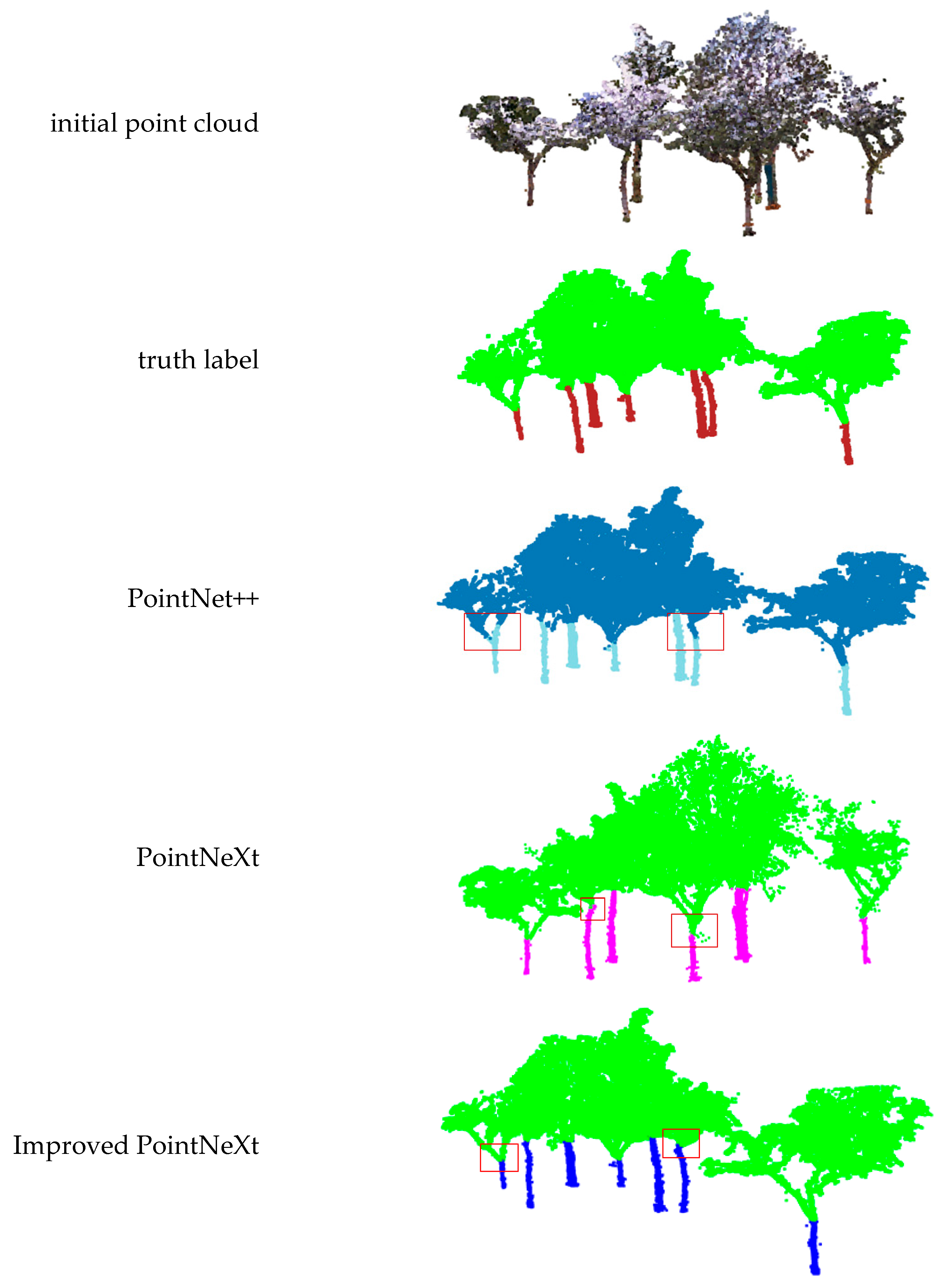
The results of different semantic segmentations are shown in Figure 16. It can be seen that the improved PointNeXt can indeed segment canopy data accurately.
In summary, the improved PointNeXt model achieves the best results among the tested semantic segmentation models with the highest segmentation accuracy.
The combined GVA and EdgeConv modules can re-learn local information and extract finer features while maintaining alignment invariance and capturing local geometric features, enabling an increase in mIoU. The model is able to more accurately identify the boundary between the canopy and the trunk when distinguishing point clouds. This increase in accuracy is crucial to understanding the tree structure. The junction between the canopy and trunk may contain a large number of overlapping points, complicating boundary identification. mIoU’s improvements show that the model is able to distinguish these points more accurately, resulting in a clear definition of the canopy and trunk in the segmentation results. The improvement of segmentation accuracy directly reduces the error in volume calculation.
In order to validate the effectiveness and generalizability of the proposed method, we conducted an experimental evaluation of the semantic segmentation on the public dataset S3DIS (Stanford Large-Scale 3D Indoor Spaces). S3DIS is composed of six large-scale indoor regions, 271 rooms, and 13 semantic categories [36]. Region 5 was used for the test evaluation in this study.
As shown in Table 4, we selected a relatively new SPoTr network from 2023 for comparison, and the mIoU obtained by the improved PointNeXt in this paper performed well, proving the effectiveness of the proposed method.

4.2. Comparison of Effects on Canopy Volume Results before and after Mean Shift Improvement

To verify the effectiveness of the improved Mean Shift algorithm, we compare canopy volume calculations before and after the algorithm’s enhancement.
(1) Keeping the Mean Shift kernel function unchanged and only replacing the k-nn search in Mean Shift with KdTree search, the improved algorithm runs in a significantly shorter time than the normal algorithm. Table 5 lists the running time of the two algorithms on top of the canopy volume calculation. However, adding a KdTree search does not change the calculation.
(2) Keeping all other conditions of Mean Shift unchanged and changing only the kernel function.
The process of Mean Shift density clustering is controlled by the size of bandwidth, since it is not clear whether this bandwidth parameter has a great influence on the results of using the TLS data to find the best results through density clustering. In this paper, the parameter is adjusted to find the best results through density clustering. In order to find the most suitable bandwidth setting, comparison experiments with different bandwidths are shown in Table 6.
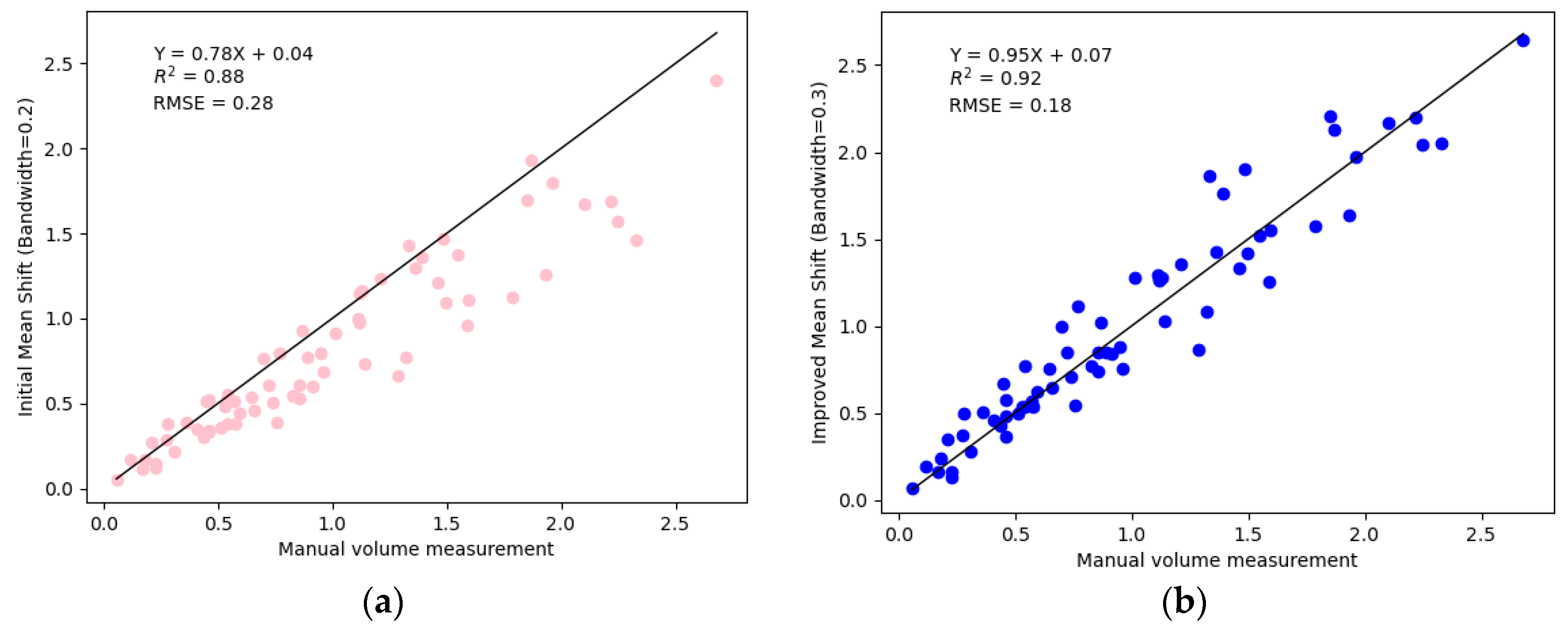
According to Table 6, too small a bandwidth leads to excessive clustering, and canopy structure information is ignored. Too large a bandwidth leads to the canopy containing too many gaps, which affects the results. The final choice is to set the bandwidth to 0.2 as the most suitable parameter. As a result, R2 is 0.88 and RMSE is 0.28 m3.
In this paper, by introducing a new kernel function and finding a suitable bandwidth parameter, the accuracy of the algorithm calculation can be effectively improved. The final choice is to set the bandwidth to 0.3 as the most suitable parameter. The best R2 and RMSE for improved Mean Shift are 0.92 and 0.18 m3.
The best results of the two algorithms use linear regression analysis, as shown in Figure 17. The results are evidence of the effectiveness of the algorithmic improvements.

4.3. Comparison of Canopy Volume Calculation by Different Methods

(1)
Acquisition of true reference values
The general true values need to be measured manually at the site, which takes a lot of time and effort. Therefore, for the convenience of measurement, this study uses the Calculate 2.5D Volume operation in the CloudCompare software to achieve accurate calculation of the point cloud volume. First, the data is imported into the software environment in a complete and accurate manner by loading the required point cloud data. Subsequently, key parameters of the Compute 2.5D Volume operation are adjusted, including but not limited to the selection of the volume calculation region and the adjustment of the calculation resolution, to ensure that the resulting volume values are as close as possible to the true values.
During the calculation process, we place special emphasis on the fine tuning of the parameters to cope with the influence of possible noise, data density variations, and other factors on the volume calculation results. By trying different parameter combinations several times, we strive to make the volume calculation results converge to the real value in order to improve the accuracy and reliability of this study. This process is repeated and iterated until converged calculation results are obtained.
(2)
Voxel-based method
The canopy space is first divided into regular square voxels, ensuring that the size of each voxel is fixed. This helps to discretize the irregularly shaped canopy. The point cloud within each small square voxel element is then counted to calculate the number of points in it. This step aims to quantify canopy structure information contained in each voxel. A threshold for the number of points in the point cloud within the small square is then set to determine which voxels are considered valid. Typically, voxels with a number of point cloud points within the small square exceeding the threshold are considered to carry enough information to be recognized as valid. Finally, the volumes of the voxels that are determined to be valid are summed to obtain a final irregular canopy volume estimate.
The formula for the area of a small square voxel is as follows:
V = a × a × a
V is the volume of a small square, and a is the length of the side of the small square in m.
This voxel-based method provides an efficient way to calculate the volume of irregularly shaped canopies. However, the choice of edge lengths of small square elements has a significant impact on the results. Large voxels might lose the internal structural details of the canopy, while small voxels might not be able to compensate for the shading effect of the canopy structure well. In the actual calculation of canopy volume, the voxel size needs to be carefully selected according to the characteristics of the canopy structure.
(3)
3D convex hull
This methodology consists of creating a minimal convex hull for the individual tree canopy point cloud data that encloses all the point clouds in 3D space, which is defined by a set of external minimal planes that wrap around the entire point cloud, performing a merge to ensure that the entire shape is convex. The volume of the convex hull is then computed using the small planes as boundaries. Its boundary consists of a number of triangles.
The schematics of the canopy volume algorithms are shown in Figure 18.
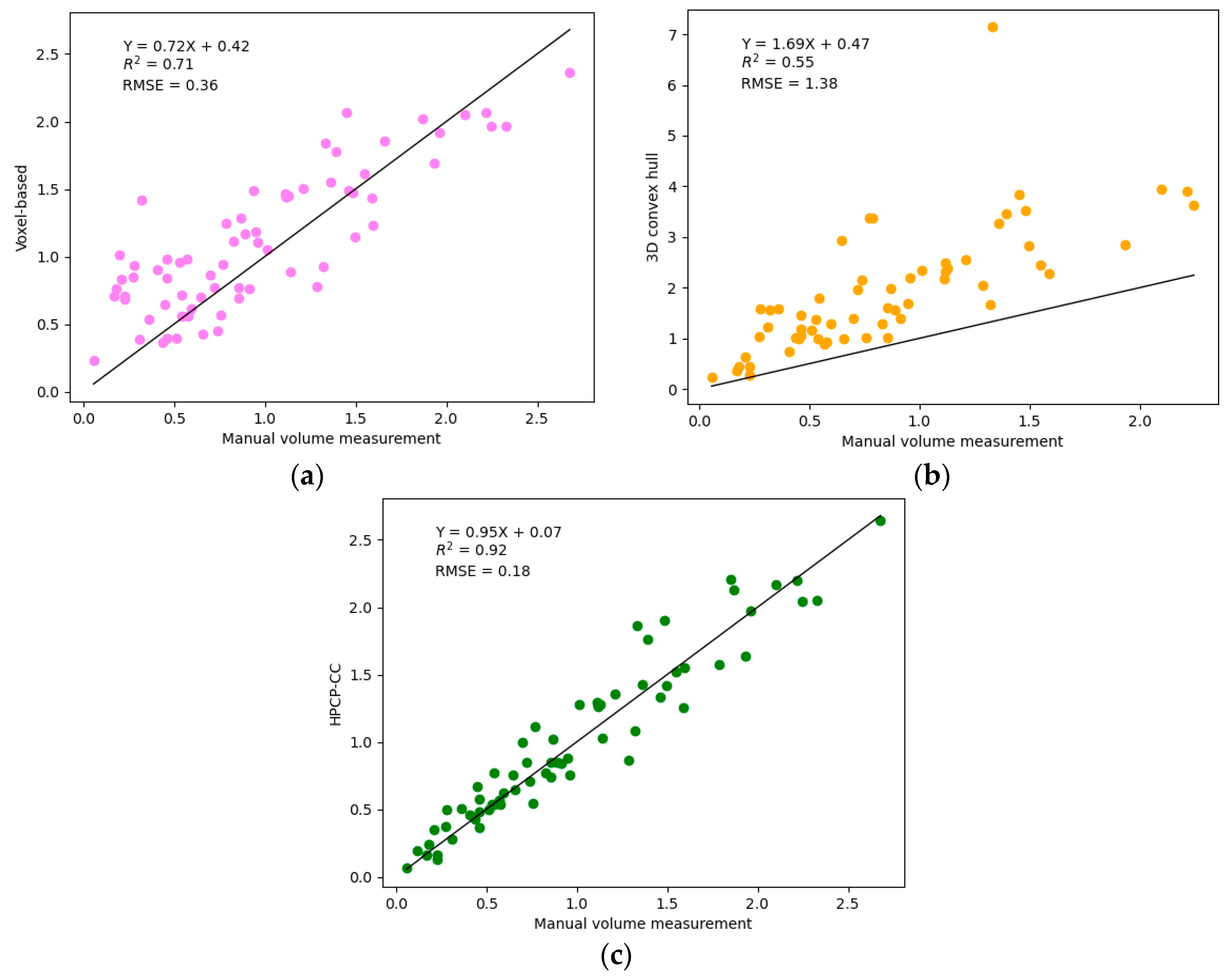
In order to verify the effectiveness of the algorithms in this paper, we compare two existing algorithms on the Baima campus dataset. In addition, to verify the robustness of the algorithms, this paper uses the Hung-tse Lake planted forest dataset for comparison, and the results are shown in Table 7.

4.4. Evaluation of Results

In order to find the best algorithm for calculating the volume of an automatically extracted individual tree canopy and to verify the accuracy of the method proposed in this paper, linear regression analyses of the three volumetric algorithms with manual measurement are performed. The manually calculated canopy volume values are taken as the true values and the results of the different volume algorithms are taken as the comparative values. As an example, the results are shown in Figure 19 for a school street tree. It can be seen that using the 3D convex hull tree volume compares to the exact value with an R2 and RMSE of 0.55 and 1.38 m3; the volume of the voxel-based algorithm tree compares to the exact value with an R2 of 0.71 and RMSE of 0.36 m3; and the improved Mean Shift clustering convex hull algorithm compares with an R2 and RMSE of 0.92 and 0.18 m3. The three-dimensional convex hull algorithm has a closed effect on the whole tree canopy, and there are too many gaps. Different parameters of the voxel-based algorithm fluctuate the point cloud volume, resulting in large fluctuations between the calculated volume and the manually adjusted parameter measurements. The volume calculation of the convex hull algorithm based on hierarchical projection clustering is the most stable, and at the same time solves the problem of the presence of large gaps in the tree canopy.

5. Discussion

The results of this study show that it is feasible to use point cloud deep learning semantic segmentation networks combined with volume calculation algorithms to automatically obtain tree canopy volumes. Our experimental data were obtained under clear and windless conditions, and the combined use of ALS and TLS made the point cloud data clearer and more complete. As a result, the tree structure is relatively clear and has low noise, providing a good basis for overall analysis and processing. Compared to manual measurements, significant time and labor savings were achieved.
Our dataset was used to validate the algorithm using different planting densities with different tree species, in addition to open-source datasets, to validate the performance of the network. Baima Campus is an urban woodland and Hung-tse Lake is a wild woodland. The density and tree species of the two woodlands are different. The methodology of this paper mainly uses the tree species of the Whitehorse School District, and the use of plantation forest data is only to verify the robustness of the volumetric algorithm. In this paper, an improved PointNeXt network is proposed. With the GVA and Edgeconv modules, local features can be extracted more finely, while global features are fused to enhance the endogenous interactions between points, thus improving segmentation accuracy. The canopy point cloud obtained using the semantic segmentation network can be directly input into the volume algorithm to improve the calculation accuracy of the canopy volume. For the volume calculation in this paper, in the Mean Shift clustering used for datasets with large density differences, the bandwidth setting needs to be dynamically adapted to the dataset, which is something that can be enhanced and optimized in future research.
Although progress has been made with the improved PointNeXt network, further optimization is needed, especially of the feature extraction module, and there is a need to continually improve the network structure to enhance the segmentation of complex tree structures and improve the accuracy and efficiency of the method and to better handle the diversity and complexity of tree structures, especially in dense or heterogeneous forests. In addition, expanding the test to cover more datasets with different forest types, canopy densities, and environmental settings is crucial for the generalizability and robustness of the automated volume calculations.
The goal of this study is to achieve accurate canopy extraction and automated collection of canopy volume. The accurate calculation of canopy volumes is critical for forest resource management. In addition, accurate calculation of the volume of each tree is the basis for assessing timber resources, estimating timber yields, signing harvesting contracts, and trading timber.

6. Conclusions

This study realizes the calculation of high-precision, automatically acquired tree canopy volumes. The method is based on ALS and TLS registration; first, the non-tree points in the point cloud are removed, and then an improved PointNeXt semantic segmentation network is used to extract the canopy data. The results show that the segmentation effect is excellent, the mIoU is 98.19%, and the training time it needs is short, fast, and also more stable. In this paper, the improved KdTree-based Mean Shift and convex hull volume algorithms have the highest R2 and RMSE of 0.92 and 0.18 m3 respectively, followed by the voxel-based method and 3D convex hull method. Therefore, the improved method in this paper is the best method for the segmentation of canopy data and the calculation of canopy volume. The following conclusions are drawn from this study.
(1)
With the help of the ICP registration algorithm in the CloudCompare software, the ALS and TLS point cloud data acquired by a 3D laser scanning system were fused and then pre-processed, and finally new point cloud data were created for segmentation and volume calculation.
(2)
In response to the poor performance of the classical semantic segmentation networks on the dataset of this study, PointNeXt was improved so as to realize the accurate segmentation of the canopy and trunk, which provided the basis for the subsequent volume calculation of the canopy.
(3)
Based on the comparison of different volume calculations’ results, the improved algorithm in this paper can effectively remove the gaps in tree canopy to better calculate canopy volume.

Author Contributions

Conceptualization, H.S. and C.H.; methodology, H.S. and C.H.; software, H.S.; validation, H.S.; analysis, H.S.; data curation, H.S. and Q.Y.; writing—original draft preparation, H.S.; writing—review and editing, H.S., Q.Y., Q.C., L.F., Z.X. and C.H.; project administration, Q.Y. and C.H.; All authors have read and agreed to the published version of the manuscript.

Funding

This work was supported by the Fundamental Research Funds for the Central Nonprofit Research Institution of CAF (CAFYBB2022ZB002) and the National Key Research and Development Program of China under Grant 2022YFD2201005-03 and the Institute of Resource Information, Chinese Academy of Forestry.

Data Availability Statement

The point cloud data used to support the findings of this study have not been made available because the data were obtained by the authors and their institutions for a fee and relate to their privacy.

Acknowledgments

We would like to thank the Advanced Analysis and Testing Centre of Nanjing Forestry University, China for their assistance with data collection and technical support.

Conflicts of Interest

All authors declare that this research was conducted in the absence of any commercial or financial relationships that could be construed as potential conflicts of interest.

References

  1. Zabret, K.; Lebar, K.; Sraj, M. Temporal response of urban soil water content in relation to the rainfall and throughfall dynamics in the open and below the trees. J. Hydrol. Hydromech. 2023, 71, 210–220. [Google Scholar] [CrossRef]
  2. Torres-sánchez, J.; Escolà, A.; de Castro, A.I.; López-Granados, F.; Rosell-Polo, J.R.; Sebé, F.; Jiménez-Brenes, F.M.; Sanz, R.; Gregorio, E.; Peña, J.M. Mobile terrestrial laser scanner vs. UAV photogrammetry to estimate woody crop canopy parameters-Part 2: Comparison for different crops and training systems. Comput. Electron. Agric. 2023, 212, 108083. [Google Scholar] [CrossRef]
  3. Zhu, Z.H.; Kleinn, C.; Nölke, N. Towards Tree Green Crown Volume: A Methodological Approach Using Terrestrial Laser Scanning. Remote Sens. 2020, 12, 1841. [Google Scholar] [CrossRef]
  4. van der Meer, M.; Lee, H.Y.R.; de Visser, P.H.B.; Heuvelink, E.; Marcelis, L.F.M. Consequences of interplant trait variation for canopy light absorption and photosynthesis. Front. Plant Sci. 2023, 14, 1012718. [Google Scholar] [CrossRef]
  5. Cai, Y.H.; Nishimura, T.; Ida, H.; Hirota, M. Spatial variation in soil respiration is determined by forest canopy structure through soil water content in a mature beech forest. For. Ecol. Manag. 2021, 501, 119673. [Google Scholar] [CrossRef]
  6. Zhang, D.C.; Dietze, M. Towards uninterrupted canopy-trait time-series: A Bayesian radiative transfer model inversion using multi-sourced satellite observations. Remote Sens. Environ. 2023, 287, 113475. [Google Scholar] [CrossRef]
  7. Lian, X.G.; Zhang, H.L.; Xiao, W.; Lei, Y.P.; Ge, L.L.; Qin, K.; He, Y.W.; Dong, Q.Y.; Li, L.F.; Han, Y.; et al. Biomass Calculations of Individual Trees Based on Unmanned Aerial Vehicle Multispectral Imagery and Laser Scanning Combined with Terrestrial Laser Scanning in Complex Stands. Remote Sens. 2022, 14, 4715. [Google Scholar] [CrossRef]
  8. Palpali, T.; Riwasino, J. Estimation of above ground biomass and carbon of pinus caribaea in bulolo forest plantation, papua new. Maderas-Cienc. Y Tecnol. 2023, 9, 1–10. [Google Scholar] [CrossRef]
  9. Feng, H.K.; Yue, J.B.; Fan, Y.G.; Yang, G.J.; Zhao, C.J. Estimation of Potato Above-Ground Biomass Based on VGC-AGB Model and Hyperspectral Remote Sensing. Spectrosc. Spectr. Anal. 2023, 43, 2876–2884. [Google Scholar]
  10. Ding, X.; Xu, Z.L.; Wang, Y. Application of MaxEnt Model in Biomass Estimation: An Example of Spruce Forest in the Tianshan Mountains of the Central-Western Part of Xinjiang, China. Forests 2023, 14, 953. [Google Scholar] [CrossRef]
  11. Korhonen, L.; Vauhkonen, J.; Virolainen, A.; Hovi, A.; Korpela, I. Estimation of tree crown volume from airborne lidar data using computational geometry. Int. J. Remote Sens. 2013, 34, 7236–7248. [Google Scholar] [CrossRef]
  12. Yan, Z.J.; Liu, R.F.; Cheng, L.; Zhou, X.; Ruan, X.G.; Xiao, Y.J. A Concave Hull Methodology for Calculating the Crown Volume of Individual Trees Based on Vehicle-Borne LiDAR Data. Remote Sens. 2019, 11, 623. [Google Scholar] [CrossRef]
  13. Ross, C.W.; Loudermilk, E.L.; Skowronski, N.; Pokswinski, S.; Hiers, J.K.; O’Brien, J. LiDAR Voxel-Size Optimization for Canopy Gap Estimation. Remote Sens. 2022, 14, 1054. [Google Scholar] [CrossRef]
  14. Jurado, J.M.; Pádua, L.; Feito, F.R.; Sousa, J.J. Automatic Grapevine Trunk Detection on UAV-Based Point Cloud. Remote Sens. 2020, 12, 3043. [Google Scholar] [CrossRef]
  15. Chavez-Duran, A.A.; Garcia, M.; Olvera-Vargas, M.; Aguado, I.; Figueroa-Rangel, B.L.; Trucios-Caciano, R.; Rubio-Camacho, E.A. Forest Canopy Fuel Loads Mapping Using Unmanned Aerial Vehicle High-Resolution Red, Green, Blue and Multispectral Imagery. Forests 2024, 15, 225. [Google Scholar] [CrossRef]
  16. Tunca, E.; Köksal, E.S. Bell pepper yield estimation using time series unmanned air vehicle multispectral vegetation indexes and canopy volume. J. Appl. Remote Sens. 2022, 16, 022202. [Google Scholar] [CrossRef]
  17. Young, T.J.; Jubery, T.Z.; Carley, C.N.; Carroll, M.; Sarkar, S.; Singh, A.K.; Singh, A.; Ganapathysubramanian, B. “Canopy fingerprints” for characterizing three-dimensional point cloud data of soybean canopies. Front. Plant Sci. 2023, 14, 1141153. [Google Scholar] [CrossRef]
  18. Escolà, A.; Peña, J.M.; López-Granados, F.; Rosell-Polo, J.R.; de Castro, A.I.; Gregorio, E.; Jiménez-Brenes, F.M.; Sanz, R.; Sebe, F.; Llorens, J.; et al. Mobile terrestrial laser scanner vs. UAV photogrammetry to estimate woody crop canopy parameters-Part 1: Methodology and comparison in vineyards. Comput. Electron. Agric. 2023, 212, 108109. [Google Scholar] [CrossRef]
  19. Qi, C.R.; Su, H.; Mo, K.C.; Guibas, L.J. PointNet: Deep Learning on Point Sets for 3D Classification and Segmentation. In Proceedings of the 30th IEEE/CVF Conference on Computer Vision and Pattern Recognition (CVPR), Honolulu, HI, USA, 21–26 July 2017; IEEE: Piscataway, NJ, USA, 2017; pp. 77–85. [Google Scholar]
  20. Qi, C.R.; Yi, L.; Su, H.; Guibas, L.J. PointNet plus plus : Deep Hierarchical Feature Learning on Point Sets in a Metric Space. In Proceedings of the 31st Annual Conference on Neural Information Processing Systems (NIPS), Long Beach, CA, USA, 4–9 December 2017. [Google Scholar]
  21. He, H.Q.; Zhou, F.Y.; Xia, Y.P.; Chen, M.; Chen, T. Parallel Fusion Neural Network Considering Local and Global Semantic Information for Citrus Tree Canopy Segmentation. IEEE J. Sel. Top. Appl. Earth Obs. Remote Sens. 2024, 17, 1535–1549. [Google Scholar] [CrossRef]
  22. Martins, J.A.C.; Nogueira, K.; Osco, L.P.; Gomes, F.D.G.; Furuya, D.E.G.; Gonçalves, W.N.; Sant’Ana, D.A.; Ramos, A.P.M.; Liesenberg, V.; dos Santos, J.A.; et al. Semantic Segmentation of Tree-Canopy in Urban Environment with Pixel-Wise Deep Learning. Remote Sens. 2021, 13, 3054. [Google Scholar] [CrossRef]
  23. Zhang, Y.Z.; Liu, H.T.; Liu, X.Y.; Yu, H.L. Towards Intricate Stand Structure: A Novel Individual Tree Segmentation Method for ALS Point Cloud Based on Extreme Offset Deep Learning. Appl. Sci. 2023, 13, 6853. [Google Scholar] [CrossRef]
  24. Xu, J.Z.; Wang, G. Segmentation of street trees from MLS point clouds by dimensional feature analysis and improved FCM algorithm. In Proceedings of the 9th Conference on Applied Optics and Photonics China (AOPC)—Advanced Laser Technology and Application (AOPC), Beijing, China, 30 November–2 December 2020. [Google Scholar]
  25. Kim, D.H.; Ko, C.U.; Kim, D.G.; Kang, J.T.; Park, J.M.; Cho, H.J. Automated Segmentation of Individual Tree Structures Using Deep Learning over LiDAR Point Cloud Data. Forests 2023, 14, 1159. [Google Scholar] [CrossRef]
  26. Hu, X.D.; Hu, C.H.; Han, J.A.; Sun, H.; Wang, R. Point cloud segmentation for an individual tree combining improved point transformer and hierarchical clustering. J. Appl. Remote Sens. 2023, 17, 034505. [Google Scholar] [CrossRef]
  27. Qian, G.; Li, Y.; Peng, H.; Mai, J.; Hammoud, H.; Elhoseiny, M.; Ghanem, B. Pointnext: Revisiting pointnet++ with improved training and scaling strategies. Adv. Neural Inf. Process. Syst. 2022, 35, 23192–23204. [Google Scholar]
  28. Engel, N.; Belagiannis, V.; Dietmayer, K. Point Transformer. IEEE Access 2021, 9, 134826–134840. [Google Scholar] [CrossRef]
  29. Kumar, S.; Sara, R.; Singh, J.; Agrawal, S.; Kushwaha, S.P. Spaceborne PolInSAR and ground-based TLS data modeling for characterization of forest structural and biophysical parameters. Remote Sens. Appl. Soc. Environ. 2018, 11, 241–253. [Google Scholar] [CrossRef]
  30. Wu, X.; Lao, Y.; Jiang, L.; Liu, X.; Zhao, H. Point transformer v2: Grouped vector attention and partition-based pooling. Adv. Neural Inf. Process. Syst. 2022, 35, 33330–33342. [Google Scholar]
  31. Phan, A.V.; Nguyen, M.L.; Nguyen, Y.L.H.; Bui, L.T. DGCNN: A convolutional neural network over large-scale labeled graphs. Neural Netw. 2018, 108, 533–543. [Google Scholar] [CrossRef]
  32. Lu, Y.C.; Cheng, L.Y.; Isenberg, T.; Fu, C.W.; Chen, G.N.; Liu, H.; Deussen, O.; Wang, Y.H. Curve Complexity Heuristic KD-trees for Neighborhood-based Exploration of 3D Curves. Comput. Graph. Forum 2021, 40, 461–474. [Google Scholar] [CrossRef]
  33. Dinh, N.T.; Le, T.M.; Van, T.T. An Improvement Method of Kd-Tree Using k-Means and k-NN for Semantic-Based Image Retrieval System. In Proceedings of the World Conference on Information Systems and Technologies (WorldCIST), Electr Network, Budva, Montenegro, 12–14 April 2022; pp. 177–187. [Google Scholar]
  34. Ameijeiras-Alonso, J.; Einbeck, J. A fresh look at mean-shift based modal clustering. Adv. Data Anal. Classif. 2023, 1–29. [Google Scholar] [CrossRef]
  35. Leibrandt, R.; Günnemann, S. Gauss Shift: Density Attractor Clustering Faster Than Mean Shift. In Proceedings of the European Conference on Machine Learning and Principles and Practice of Knowledge Discovery in Databases (ECML PKDD), Electr Network, Ghent, Belgium, 14–18 September 2020; pp. 125–142. [Google Scholar]
  36. Armeni, I.; Sener, O.; Zamir, A.R.; Jiang, H.; Brilakis, I.; Fischer, M.; Savarese, S. 3D Semantic Parsing of Large-Scale Indoor Spaces. In Proceedings of the 2016 IEEE Conference on Computer Vision and Pattern Recognition (CVPR), Seattle, WA, USA, 27–30 June 2016; IEEE: Piscataway, NJ, USA, 2016; pp. 1534–1543. [Google Scholar]
  37. Park, J.; Lee, S.; Kim, S.; Xiong, Y.; Kim, H.J. Self-positioning point-based transformer for point cloud understanding. In Proceedings of the IEEE/CVF Conference on Computer Vision and Pattern Recognition, Vancouver, BC, Canada, 17–24 June 2023; pp. 21814–21823. [Google Scholar]
Figure 1. Geographic location map of the study area.
Remotesensing 16 02641 g001
Figure 2. Field scanning scene.
Remotesensing 16 02641 g002
Figure 3. Distribution of foundations of the 17 stations in the sample site.
Remotesensing 16 02641 g003
Figure 4. Raw point cloud data. (a) TLS point cloud. (b) ALS point cloud.
Remotesensing 16 02641 g004
Figure 5. Overall framework.
Remotesensing 16 02641 g005
Figure 6. Point cloud data after registration.
Remotesensing 16 02641 g006
Figure 7. Filtering results of tree point cloud. (a) Original tree point cloud. (b) Filtered and denoised tree point cloud.
Remotesensing 16 02641 g007
Figure 8. Extraction of tree results. (a,b) Including brackets, people, and weeds. (c,d) Pretreated to contain no weeds.
Remotesensing 16 02641 g008
Figure 9. The result of PointNet++.
Remotesensing 16 02641 g009
Figure 10. Overall network structure of the improved PointNeXt model.
Remotesensing 16 02641 g010
Figure 11. Grouped vector attention block.
Remotesensing 16 02641 g011
Figure 12. Group coding function.
Remotesensing 16 02641 g012
Figure 13. EdgeConv block.
Remotesensing 16 02641 g013
Figure 14. EdgeConv Calculation Principle.
Remotesensing 16 02641 g014
Figure 15. Parts of the dataset. (a) area1, (b) area2, (c) area3, (d) area4, (e) area5, and (f) area6.
Remotesensing 16 02641 g015
Figure 16. Semantic segmentation results.
Remotesensing 16 02641 g016
Figure 17. Comparison of before and after improvement. (a) Based on initial Mean Shift. (b) Based on improved Mean Shift.
Remotesensing 16 02641 g017
Figure 18. Different methods of presentation. (a) Voxel-based. (b) 3D convex hull. (c) HPCP-CC.
Remotesensing 16 02641 g018
Figure 19. Scatter plots of the three algorithms compared to the volume obtained from manual measurement of the true value. (a) Voxel-based. (b) 3D convex hull. (c) HPCP-CC.
Remotesensing 16 02641 g019
Table 1. Technical Data: Trimble TX7 Laser Scanning.
Performance Trimble TX7
Scanning speed500,000 dots per second
Scanner weight5.8 kg
Measurement accuracy1 mm
Distance range80 m
Scanning time of a single scanning job10 s to 3 min
Scanning PrincipleScanning Tape with a Rotating Pris
Table 2. The list of data used for validation included density, diameter at breast height (DBH), tree height, and number of trees.
LocationStem Density
(Number/ha)
DBH (mm)Tree Height (m)Number of Trees Selected
AverageMinMaxAverageMinMax
Baima39098351913.41.86.5150
Hung-tse 4101927731120.416.523.580
Table 3. Performance of segmentation results.
MethodLatency (ms)mIoU(%)
PointNet8162.50
PointNet++6695.60
PointNeXt7197.19
PointNeXt+GVA7397.81
PointNeXt+Edgeconv7297.76
Improved PointNeXt (GVA+Edgeconv)7698.19
Table 4. Semantic segmentation results on S3DIS.
MethodmIoU (%)
SPoTr [37]70.8
PointNeXt70.5
Improved PointNeXt71.1
Table 5. Comparison of running time of Mean Shift clustering algorithm before and after improvement.
Number of CanopyOriginal Method (s)Improved Method (s)Reduction (%)
116.2912.8920.87
223.2118.1221.93
343.3734.6120.20
Table 6. Comparing Mean Shift under different bandwidths, before and after its improvement.
MethodNumber of CanopyEvaluation IndicatorsBandwidth
0.010.10.20.30.4
Initial150R2
RMSE (m3)
0.79
0.60
0.85
0.43
0.88
0.28
0.86
0.67
0.61
1.99
Improved150R2
RMSE (m3)
0.71
0.63
0.86
0.36
0.89
0.25
0.92
0.18
0.68
1.87
Table 7. Result comparison of different methods under different datasets.
DatasetNumber of CanopyEvaluation IndicatorsMethods
Voxel-Based3D Convex HullHPCP-CC
Baima150R2
RMSE (m3)
0.71
0.36
0.55
1.38
0.92
0.18
Hung-tse Lake80R2
RMSE (m3)
0.68
0.82
0.53
1.51
0.89
0.53
Disclaimer/Publisher’s Note: The statements, opinions and data contained in all publications are solely those of the individual author(s) and contributor(s) and not of MDPI and/or the editor(s). MDPI and/or the editor(s) disclaim responsibility for any injury to people or property resulting from any ideas, methods, instructions or products referred to in the content.