Abstract
Calibrating optical sensors has become a priority to maintain data quality and ensure consistency among sensors from different agencies. Achieving and monitoring radiometric calibration often involves the identification of temporally stable targets on the Earth’s surface. Although some locations across North Africa have traditionally been used as primary targets for calibration purposes, it is crucial to explore alternative options to account for potential changes in these sites over time. This study conducted a global assessment of pixel-level temporal stability using Landsat 8 OLI data, with the primary goal of identifying regions suitable for global radiometric calibration efforts. This work followed a two-stage approach, including the testing and selection of an effective combination of statistical tests to differentiate between temporally stable and unstable pixels and the generation of a worldwide mosaic of temporally stable pixels through a per-pixel statistical analysis employing a combination of Spearman’s rho and Pettitt’s test for assessing long-term trends and detecting change points. Notably, comparing the temporal mean top-of-atmosphere (TOA) reflectance before and after applying the generated temporal filter to a site with documented unstable pixels revealed a substantial reduction in mean variation, up to 6%. In addition, slopes observed in the pre-filter mean TOA reflectance, ranging between −0.002 and −0.005, became zero or near-zero and statistically insignificant after the temporal filter was applied, demonstrating a reduction in total uncertainties by 3 to 4%. These findings evidence the potential of this work, placing it as a potential foundation in the continuous search to identify additional targets for global radiometric calibration efforts.
1. Introduction
Over the past five decades, advancements in remote sensing have significantly improved the role of satellite imagery in enhancing the understanding of changes on the Earth’s surface. However, accurate quantitative applications like monitoring climate change, tracking wildfires, managing natural resources, and assessing agriculture depend heavily on well-calibrated sensors. Consequently, implementing periodic radiometric calibration for these optical sensors is required [1,2,3,4].
Although some of these sensors undergo thorough radiometric calibration before launch, there is a possibility of gradual degradation once they are in orbit [5]. A cost-effective and reliable approach to ensuring the maintenance of radiometric calibration for optical sensors on board satellites involves vicarious calibration using stable targets on the Earth’s surface. Traditionally, small regions across the Sahara Desert have been used for this purpose; these regions are called pseudo invariant calibration sites (PICSs) [6,7,8,9]. Cosnefroy et al. performed a characterization of desert sites in North Africa and Saudi Arabia for the calibration of optical satellite sensors. In that work, the authors identified 20 regions of 100 × 100 km2 in size using a criterion of spatial uniformity, temporal stability, accessibility, and meteorological conditions [10]. In addition, Helder et al. [11] developed an algorithm to automatically identify statistically favorable sites with stable temporal characteristics around the world. The authors found six optimal sites in the Sahara and Middle East regions, with variability of approximately 2% in the visible and near-infrared (VNIR) and 2–3% in the short-wavelength infrared (SWIR) regions. The Sonoran Desert site in North America, backed by historical calibration data, also exhibited similar potential. Additionally, sites in China and Argentina are promising candidates, particularly for SWIR monitoring.
Previous studies have indicated that PICS locations exhibit temporal stability, and Tuli’s [12] work expanded this by assessing the temporal stability of six distinct PICSs across North Africa. The authors used a “virtual constellation” involving four sensors: the Operational Land Imager (Landsat 8-OLI), Enhanced Thematic Mapper Plus (Landsat 7-ETM+), Moderate Resolution Imaging Spectroradiometer (MODIS—Terra and Aqua), and a multispectral instrument (Sentinel 2A) to ensure broader temporal coverage and to avoid relying on the characteristics of a single sensor. Using the nonparametric seasonal Mann–Kendall test, that study aimed to identify trends in reflectance measurements and evaluate the temporal stability of PICSs.
The findings of that study demonstrated that Libya 4 and Egypt 1 did not show a monotonic trend across six reflective solar bands, confirming their temporal stability. Conversely, Sudan 1 exhibited a consistent decreasing trend across all bands except for the SWIR 2 band. In addition, for Niger 1, a decreasing trend was observed in the green and red bands, while Niger 2 exhibited an increasing trend in the blue band. Khadka et al. [13] further assessed the temporal stability of these PICSs by also identifying change points in the time series collected by Landsat 8-OLI, Landsat 7-ETM+, MODIS (Terra and Aqua), and Sentinel-2A. The results identified statistically significant trends and abrupt changes across all the examined sites. However, the magnitude of these trends was marked by a maximum annual TOA reflectance change of 0.215%.
Qiao et al. [14] took Tuli and Khadka’s work as a baseline to evaluate the temporal stability of test sites within the Radiometric Calibration Network (RadCalNet). That study analyzed the short and long-term radiometric trends of Gobabeb, Baotou, Railroad Valley Playa, and La Crau sites using bottom-of-atmosphere (BOA) reflectance as well as TOA reflectance. The authors found that the trends based on TOA reflectance sometimes differed from those based on BOA reflectance. For example, while the TOA reflectance showed a significant downward trend, the red-band BOA reflectance for La Crau and Baotou in summer and autumn shift was not statistically significant. In addition, during the winter and spring seasons, the SWIR 2 band of La Crau and Baotou experienced an annual variation of 1.8%, while the SWIR 1 band of Railroad Valley Playa exhibited a change exceeding 0.3% per year. These shifts could potentially create challenges for effectively identifying sensor-specific variations when using these sites.
Given the potential changes in traditionally used calibration sites, it is imperative to actively try to identify other regions that could exhibit temporal stability on a global scale. As mentioned earlier, in the context of remote sensing, especially in the field of radiometric calibration, the detection of trends and change points in time series can be helpful in identifying regions of temporal instability. If these regions are used in stability monitoring or calibration, it could lead to false drift detection in the sensor’s response and failure to accurately describe the sensor’s behavior [15]. Areas identified as lacking trends or change points could be considered temporally stable and suitable for radiometric calibration and stability monitoring of optical satellite sensors. It is important to remember that a trend is a substantial shift over time displayed by a random variable that can be identified using statistical parametric and non-parametric techniques [16]. As previously mentioned, a temporally stable target is required for radiometric calibration and stability monitoring of optical satellite sensors; a global mosaic of temporally stable pixels could be a useful tool to identify regions with potential for radiometric calibration on a global scale.
This research goes beyond desert sites to conduct a global analysis encompassing regions with a wide range of spectral characteristics, while prioritizing temporal stability. Utilizing a per-pixel analysis of L8-OLI data on a global scale, the primary objective was to identify regions for both radiometric calibration and stability monitoring of optical satellite sensors. Deliberately excluding areas marked by substantial temporal fluctuations, this study strategically narrowed its focus to regions displaying notable global-scale temporal stability.
2. Methodology
This section presents a description of the statistical tests employed for detecting change points and long-term trends. Moreover, it provides a detailed account of the steps taken to generate data cubes, which were utilized to evaluate pixel stability on a global scale.
2.1. Statistical Tests for Change Point and Long-Term Trend Detection
Several techniques have been developed over the years to identify change points and trends in time series; some of those techniques were evaluated to identify an efficient and accurate way to detect temporally stable regions around the world. Here, six different tests were evaluated: (1) linear regression, (2) Spearman’s rho test, and (3) the Mann–Kendall test were used to evaluate long-term trends; on the other hand, (4) Pettitt’s test, (5) quadratic model fitting, and (6) cumulative sum control charts were used for detection of change points. Concise descriptions of these tests follow.
- Mann–Kendall Test:
The Mann–Kendall test is a non-parametric test developed by Mann and Kendall and is used to detect long-term trends in a time series. The statistics of the tests are not directly based on the values of the variable but rather on the signs of differences [17]. When performing the Mann–Kendall test, the data are ranked with respect to time, and each data point is used as the standard for the data points from subsequent time periods [18]. Kendall’s S is:
and
where and are the observations at times i and j, respectively, and n is the length of the time series data collection. In addition, the test statistic (S) is considered approximately normal when the number of observations used is equal to or higher than eight (n ≥ 8). In this test, mean and variance are computed according to the following equations:
where n represents the length of the time series, t is the extent of a given tie, and represents the summation of all number values within a tie. In addition, the standardized test statistics can be computed as follows [18]:
In this test, the null hypothesis (Ho no trend is present) is rejected if a positive (positive trend) or negative (negative trend) Z value is obtained. Finally, the absolute value of Z is computed and compared with the standard normal cumulative value of at p% selected significance level in order to finally decide whether the detected result is significant or not [19].
- Spearman’s rho test:
Spearman’s rho test is a non-parametric test widely used to perform trend analysis of time series. In this test, the null hypothesis Ho is that all observations are independent, and all rank orders have the same likelihood, while the alternative hypothesis H1 is that a positive or negative trend is present [20]. In this statistical analysis, Spearman’s , variance and Z statistics are calculated as follows:
where n is the number of observations and di is the rank for all observations [21].
- Linear regression and quadratic model fit:
In order to identify potentially significant trends or changes in time series, a combination of linear and quadratic regressions can be applied to a dataset within a given time frame. Linear regression can capture potential changes over time as well as at the beginning or end of the time series, whereas quadratic regression can allow the identification of changes toward the center of the time series. The significance of changes identified through linear and quadratic regressions can be evaluated using a 95% confidence level; when the confidence interval does not contain zero, it can be deduced that there is a statistically significant relationship [22]. Linear and quadratic regression models and confidence levels are estimated as follows:
where m is the slope and b is the intercept. In addition, is the sample mean, refers to the statistics from the t distribution for a 95% confidence level, and SE is the standard error of the sample mean [23].
- Pettitt’s test:
For the purpose of locating change points in a time series, several statistical tests have been developed. The change-point detection technique known as Pettitt’s test is a non-parametric test developed by Pettitt in 1979 [24]. This test is known for its ability to detect significant changes towards the center of a time series, particularly when the timing of the change is unknown. This test is based on the Mann–Whitney two-sample test (rank-based), where the null hypothesis is that no change is present in the time series. The KT statistics of the null hypothesis are shown as follows [25]:
where
refers to the statistics that show whether two samples x1…xt and xt + 1…xT belong to the same population. In addition, the significance probability of p ≤ 0.05 is described as follows:
- CUSUM control chart:
Cumulative sum control charts (CUSUMs) represent a technique widely used in industries, finance, deforestation, and crime analysis, among other fields [26]. This technique uses measurements acquired over a given timeframe to evaluate a variable’s deviation from its mean, allowing detection of both abrupt and slow changes. The cumulative sum in this test is the cumulative sum of the differences between the values and the mean; control of the upper and lower controlling limits are given as follows:
where initial values and are zero, the reference value K = kσ, usually expressed as one-and-a-half times the magnitude of the shift δ, that is, K = 0.5δσ, where the magnitude of the shift is expressed in standard deviation units. The process is regarded as being out of control if either or surpass the decision interval H = hσ [27,28].
2.2. Data Processing
In this study, which focused on creating a global mosaic of temporally stable pixels, two key data-processing stages were implemented. In the first stage, data cubes containing all available Landsat 8-OLI data were generated. Results obtained from the application of statistical tests to these data cubes were used to obtain a reference mask to select the most suitable statistical test for evaluating temporal stability at the pixel level on a global scale. Since these data cubes contained all the available data for each pixel, they were well suited for statistical testing.
In the second stage, a global dataset was created to evaluate temporal stability. Although the data cubes used in this stage were similar to those generated in the first stage, data reduction was necessary due to the large quantity of data required for a global evaluation. The statistical test evaluation using these data cubes was then compared with the statistical analysis results obtained in the first stage. For both stages, three regions of interest (ROIs) in different regions in the world and with distinct temporal and spectral characteristics were selected for testing purposes. Additional details regarding stages one and two are described in the following sections.
2.2.1. Selection of Regions of Interest (ROIs) for Testing
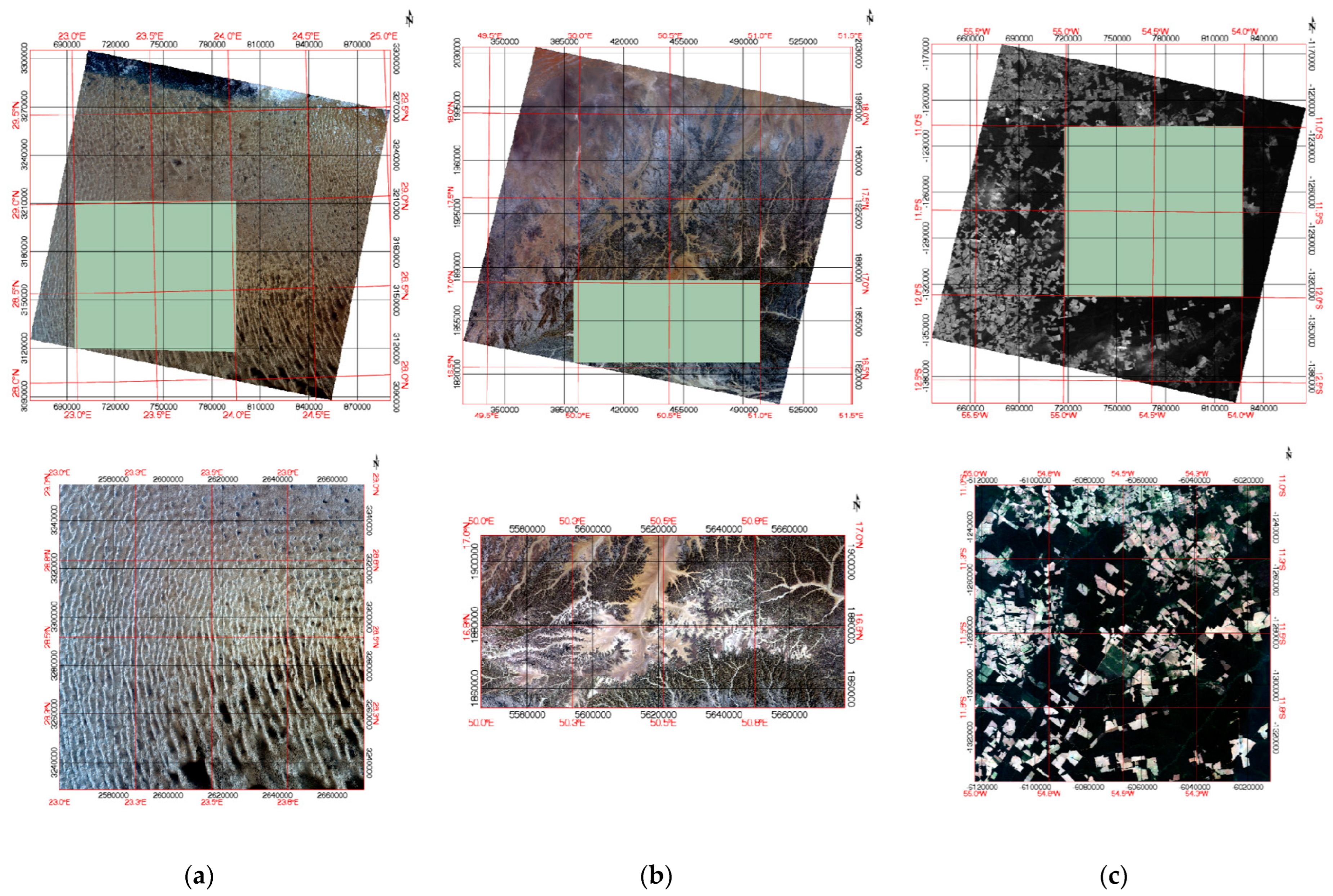
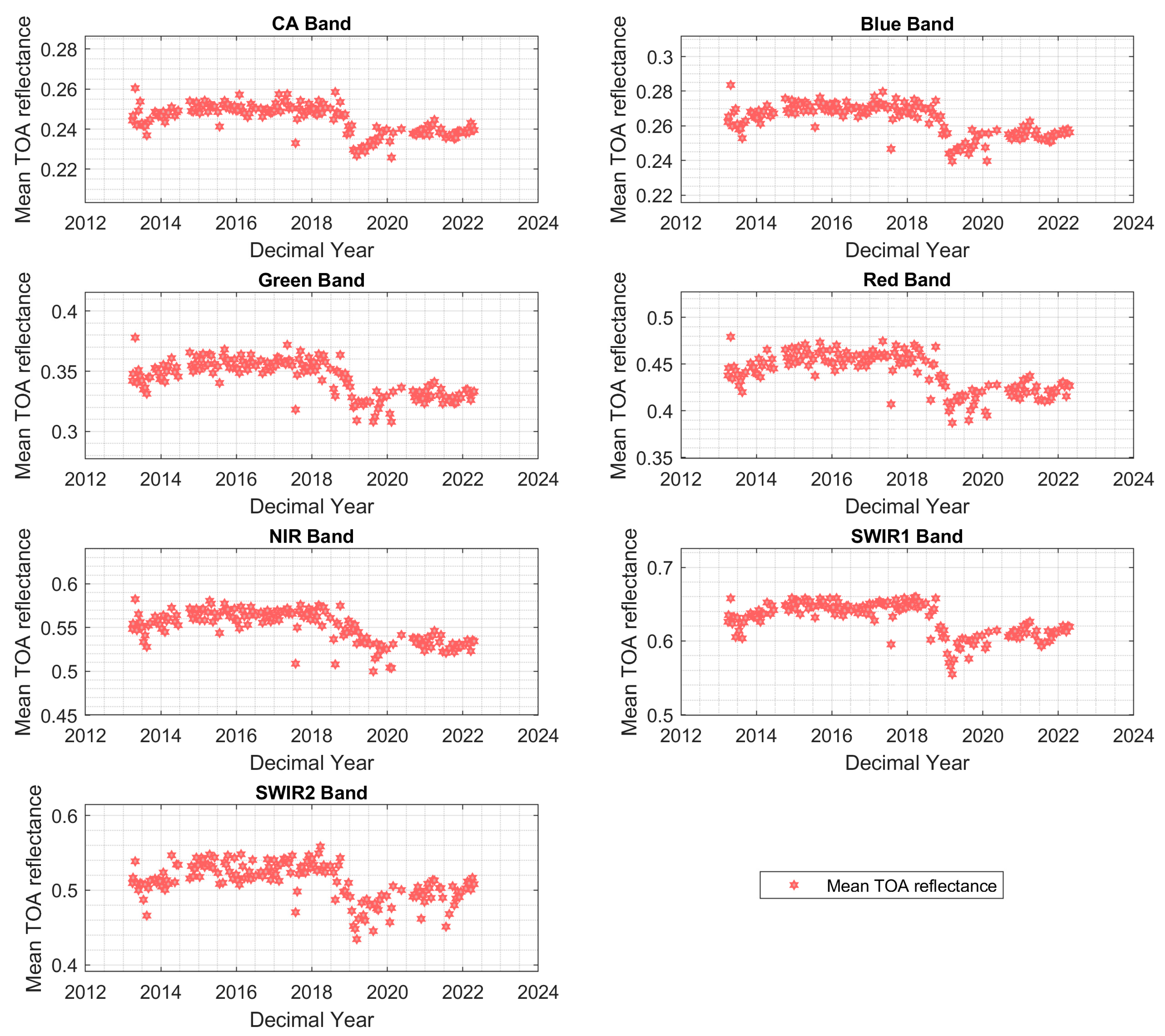
In order to identify the statistical test(s) that had the best performance with data used in this study, three ROIs were selected for testing purposes. Region 1 (ROI-1) is a homogeneous temporally stable region located within WRS-2 path 181/row 40 (Figure 1a), the same WRS-2 path/row and region where Libya 4 -CNES ROI is located. Region 2 (ROI-2) is an area containing known unstable pixels with bright spectral characteristics, located in the Middle East (WRS-2 path 162/row 48), as shown in Figure 1b. This location was initially identified by Fajardo et al. in a global land cover classification, in a search for regions suitable for radiometric calibration [29]. Temporal mean TOA reflectance exhibited a change in reflectance values for all bands after the year 2019, as shown in Figure 2. The third and last region, ROI-3 (Figure 1c), is located in Brazil, with vegetation and crop cover (WRS-2 path 226/row 68) and exhibiting a combination of stable and unstable pixels as well as different spectral characteristics compared with ROI-1 and ROI-2.
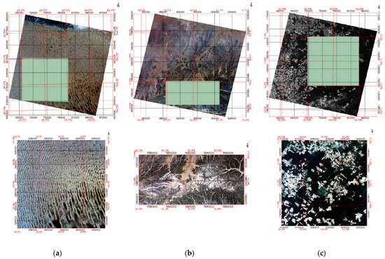
Figure 1.
Regions selected for testing: (a) green box representing ROI-1 with its corresponding RGB image, containing temporally stable pixels; (b) the green box represents ROI-2 with its corresponding RGB image, containing temporally unstable pixels; (c) green box representing ROI-3 with its corresponding RGB image, a vegetation site containing both temporally stable and unstable pixels; these ROIs were chosen to test the effectiveness of long-term trend analysis and change detection. In all images, the UTM grid is depicted in black, and lat/long is depicted in red.
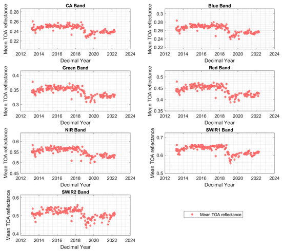
Figure 2.
TOA reflectance for WRS-2 path162/row 48 using Landsat 8 OLI, CA (430–450 nm), blue (450–510 nm), green (530–590 nm), red (640–670 nm), near-infrared (850–880 nm), SWIR 1 (1570–1650 nm), and SWIR 2 (2110–2290 nm).
2.2.2. Data Processing Using All Available Landsat 8-OLI Data (Stage 1)
Generation of Testing Data Cubes with All Available Landsat 8-OLI Data
Proceeding with the evaluation approach of finding the most suitable statistical test for this study, data cubes containing TOA reflectance were generated for each ROI using all available Landsat 8-OLI collection 2 level 1 data from February 2013 to February 2022. The data were downloaded from the United States Geological Survey (USGS) Earth Explorer website (earthexplorer.usgs.gov). The Landsat 8-OLI satellite was chosen for its proven reliability and accuracy in capturing high-quality data and its nearly decade-long data coverage across the globe. Blue, near-infrared (NIR), and short-wavelength infrared (SWIR2) bands were selected for this study to evaluate the temporal stability of the atmosphere and the ground. ROI-1, ROI-2, and ROI-3 had 191, 171, and 50 layers, respectively, for each spectral band, as shown in Figure 3. ROI-3 had substantially fewer observations than ROI-1 and ROI-2 because only images marked by USGS as having less than 10% of clouds had been downloaded to the South Dakota State University Image Processing Laboratory (SDSU IP LAB) archive. From these cubes, each layer represented a Landsat 8-OLI observation of each ROI over time. Conversion from digital numbers (DN) to NIST traceable TOA reflectance units was obtained using the following equation provided by the USGS [30]:
where and are the multiplicative and additive scaling factors, is the quantized and calibrated product for the pixel values (DN), and represents the solar zenith angle for every pixel. Multiplicative and additive factors, as well as the quantized calibrated product for the DN values, were obtained from the metadata file, and angular information was obtained from the solar- and view-angle products.

Figure 3.
Data cube structures generated using all Landsat 8-OLI data available from February 2013 to February 2021 for the NIR band.
Filtering Process Using the Pixel Quality Assessment Band Data
Cloud filtering in the process of achieving a global mosaic of temporally stable pixels relied at both stages followed in this study on the quality control band provided in the Landsat 8 OLI collection 2 level 1 product.
In the generation of ROIs for testing, as described in Section Generation of Testing Data Cubes with All Available Landsat 8-OLI Data, cloud filtering involved two steps. Initially, all images marked by USGS with 10% or more cloud coverage were rejected and not downloaded into the SDSU IP LAB archive. Additionally, a second cloud filter assessed cloud cover specifically over the ROIs. This filter utilized the quality control band provided in the Landsat 8 OLI product, employing per-pixel cloud filtering based on bit information from Bits 0, 1, 2, 3, 4, 9, 11, and 15, corresponding to fill values, dilated cloud, cirrus, cloud, cloud shadow, cloud confidence, cloud shadow confidence, and cirrus confidence, respectively. The resulting binary mask was then applied to each layer of the data cubes to ensure that the per-pixel time series included only cloud-free data. Additional information about the quality control band can be found at https://www.usgs.gov/media/files/landsat-8-9-olitirs-collection-2-level-1-data-format-control-book (accessed on 1 January 2022).
Figure 4a displays an image of WRS-2 path 181/row 40 in North Africa, visibly contaminated by clouds. The cloud binary mask generated for this scene, as described earlier, is presented in Figure 4b. In this figure, white areas indicate cloud-free pixels (value of 1), while black represents cloudy pixels (including fill pixels around the image). The cloud mask effectively removed both clouds and cloud shadows from the image.
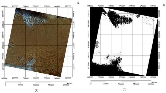
Figure 4.
Example cloud mask over path 181/row 40: (a) the RGB image over the location; and (b) the resulting cloud binary mask for the same region.
In a similar manner, for the data cubes generated for the global analysis described in Section Generating Global Data Cubes Using Google Earth Engine (GEE). the provided quality control band for the level 1 Collection 2 product available in the GEE platform was applied during the data cubes’ generation process to remove pixels contaminated by clouds.
Pixel Level BRDF Normalization Using a 4-Angle Model
BRDF effects were managed differently depending on the dataset used at each stage of this process. For instance, the data cubes generated in Section 2.2.1 for each ROI contained per-pixel time series. However, these time series exhibited a seasonal effect. This seasonal effect was attributed mainly to the bidirectional reflectance distribution function (BRDF) of the target. The substantial variation in the sun’s position across several seasons caused the majority of this BRDF variability. In order to reduce the seasonality effect, the 4-angle BRDF model developed in the SDSU IP LAB was generated and applied to each pixel [31]. BRDF-normalized time series were stored in new data cubes for the three ROIs used in this study. The 4-angle BRDF model is shown below:
where ,,, represent the Cartesian coordinates projected from the angular information in spherical coordinates, to are the coefficients in the model, and corresponds to the predicted TOA reflectance. The Cartesian coordinates used for this model were as follows:
where, SZA and SAA correspond to the solar zenith and azimuth angles and VZA and VAA correspond to the view zenith and azimuth angles.
To calculate the normalized TOA reflectance, the following equation was applied:
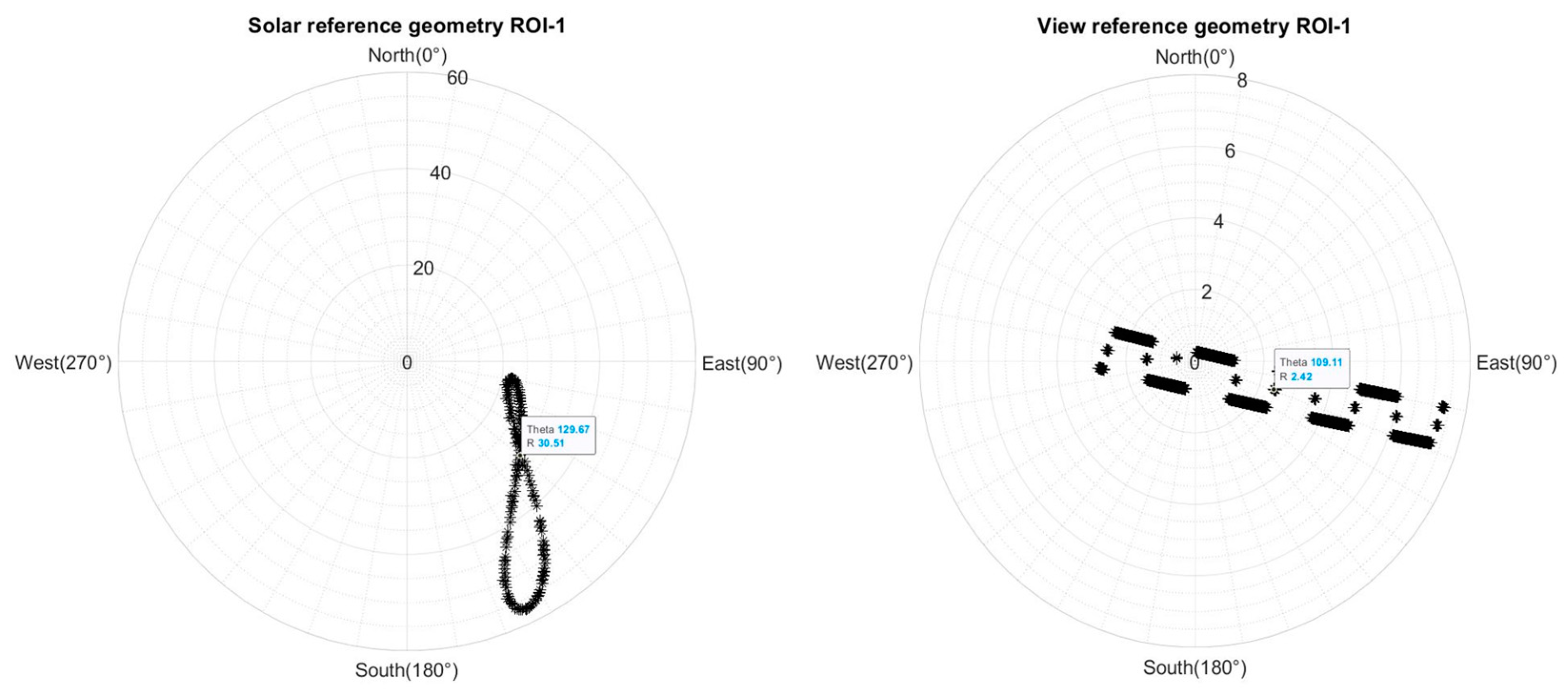
where is the resulting BRDF-normalized TOA reflectance, is the Landsat 8-OLI TOA reflectance, corresponds to the TOA reflectance predicted by the BRDF model, and is the reference reflectance estimated using a reference geometry of acquisition (solar and view geometries). For the solar reference geometry, a polar plot was used to display the solar geometry for a single randomly chosen pixel over time; the center value was selected as the reference solar geometry. In addition, the view geometry of the same scene for which the solar geometry was chosen was displayed using a polar plot. The center value in the polar plot was selected as the reference view geometry for each ROI. In this work, all pixels in each ROI were normalized to a reference reflectance computed using that acquisition reference geometry. An example of the reference geometry selection for ROI-1 is shown in Figure 5, where SZA = 30.51, SAA = 129.67, VZA = 2.42, and VAA = 109.11.

Figure 5.
Example of reference geometry selection for reference reflectance estimation for ROI-1.
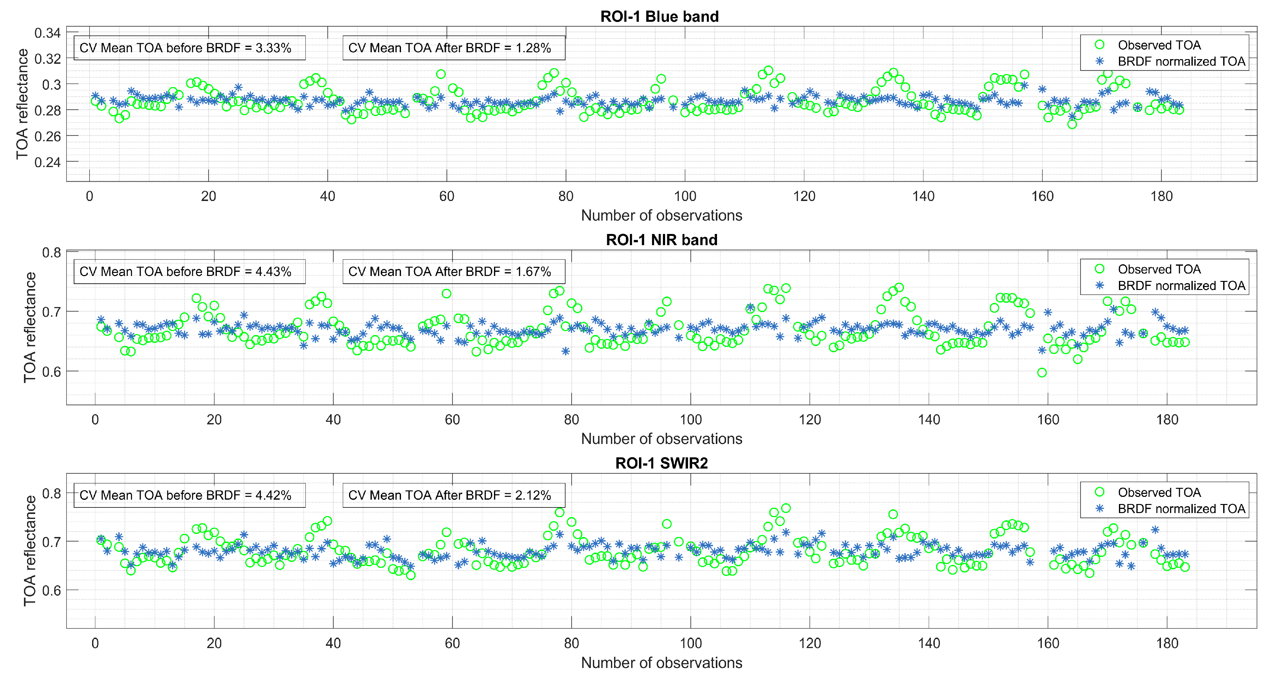
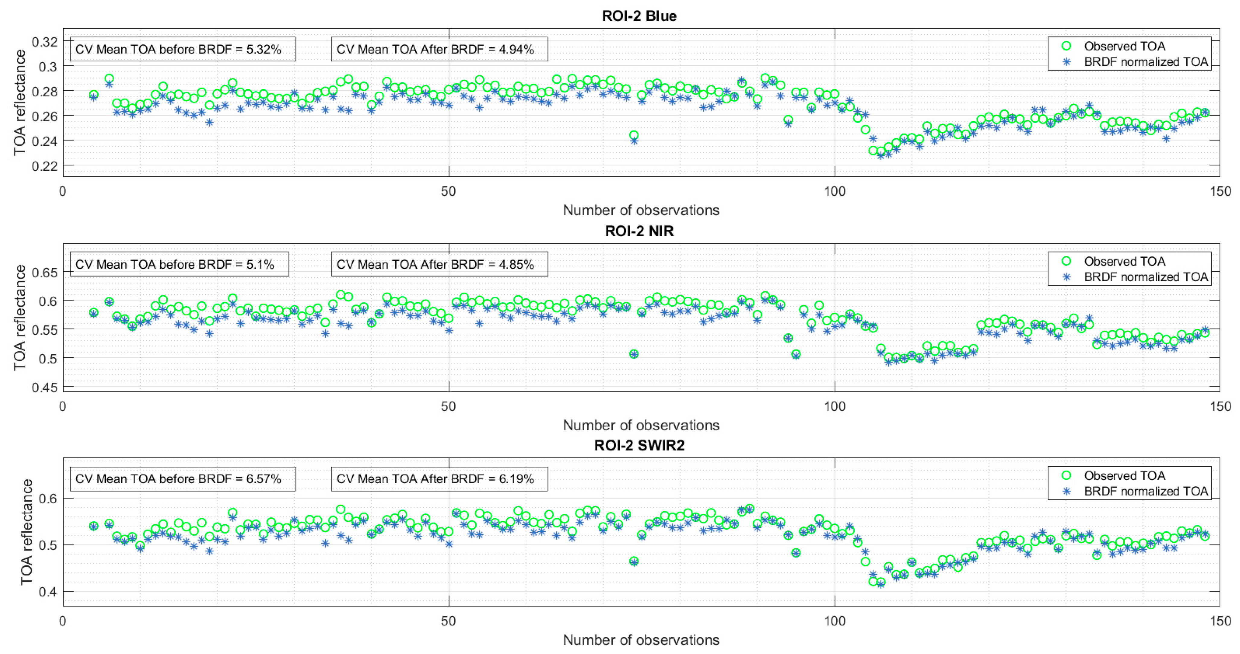
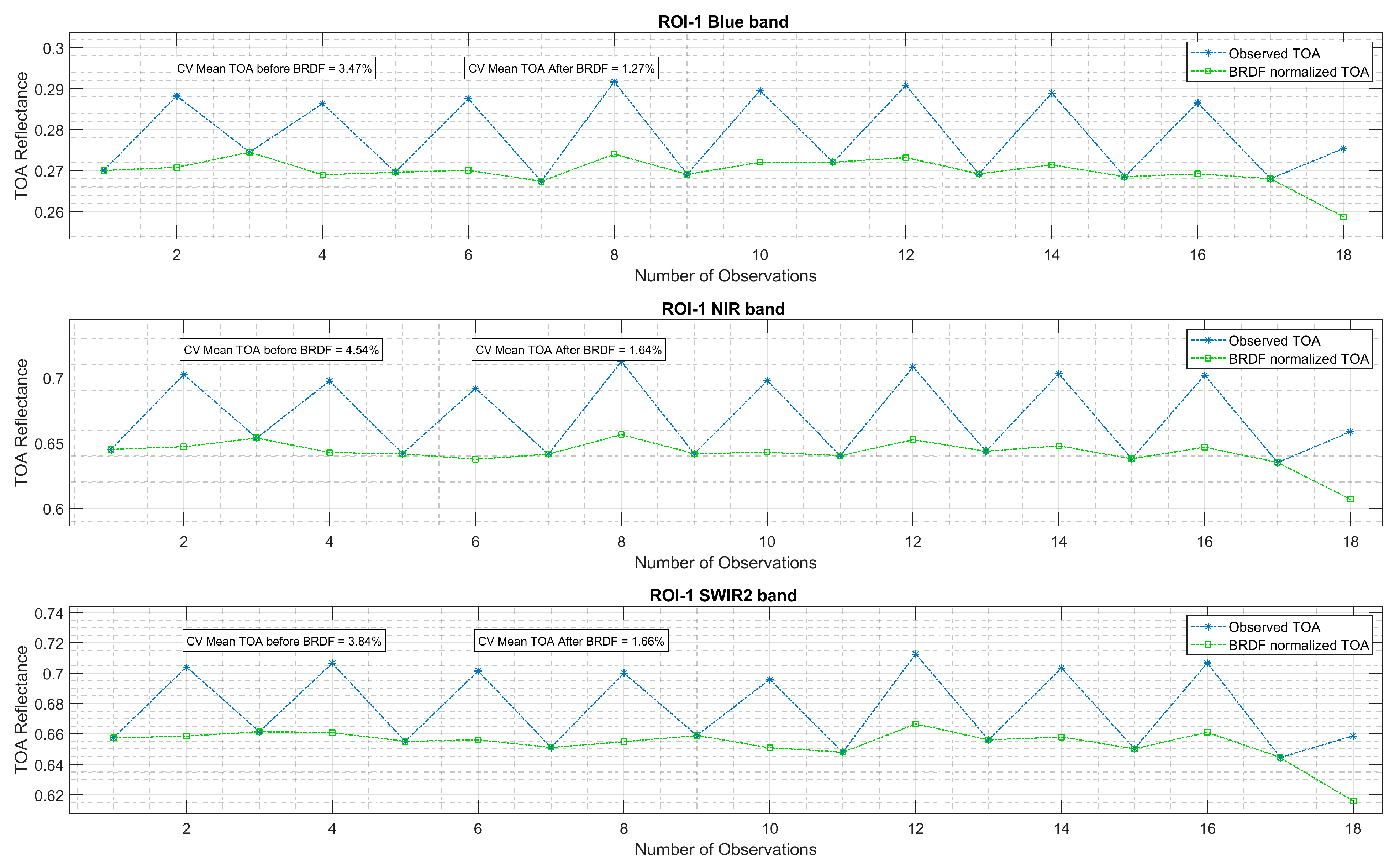
An example of the BRDF normalization is presented in Figure 6 (temporal mean TOA reflectance of a randomly selected pixel from ROI-1 using all the data available in the SDSU IP LAB archive), which includes known temporally stable pixels such as those from the Libya 4-CNES ROI. In the figure, the original observed mean TOA reflectance is represented in green, while the BRDF-normalized mean TOA reflectance is shown in blue. The seasonality effect, particularly noticeable in the NIR band, can be observed for this pixel. However, the BRDF-normalized data demonstrated a reduction in the seasonality effect in the same band. To quantify this reduction, the coefficient of variation (CV), expressed as a percentage, is included in the charts. The CV is estimated as the ratio of the standard deviation of the temporal mean TOA reflectance to the mean of the temporal mean TOA reflectance for the given pixel. The decrease in CV indicates a reduction in the seasonality effect within the pixel time series.
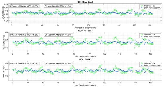
Figure 6.
Temporal mean TOA reflectance of a randomly selected pixel from ROI-1 using all the data available in the SDSU IP LAB archive.
In addition, an example of BRDF application on a pixel in the Middle East region, demonstrating temporal instability and characterized by predominantly sand and rock land cover, is shown in Figure 7 (temporal mean TOA reflectance of a randomly selected pixel from ROI-2 using all the data available in the SDSU IP LAB archive). It can be observed that the seasonal effect was less pronounced compared with the pixel shown in Figure 6. The reduction in the CV further indicated a decrease in the seasonality effect for this location. Importantly, the BRDF application did not change the inherent temporal behavior of the time series; instead, it reduced the seasonal effect while maintaining the pixel’s temporal characteristics. These temporal characteristics were later evaluated through statistical analysis, as described in Section 2.3.
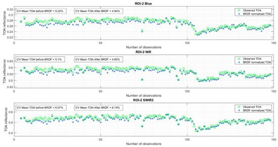
Figure 7.
Temporal mean TOA reflectance of a randomly selected pixel from ROI-2 using all the data available in the SDSU IP LAB archive.
2.2.3. Data Processing Using Global Data (Stage 2)
Generating Global Data Cubes Using Google Earth Engine (GEE)
To achieve a comprehensive assessment of temporal stability, it would have been ideal to utilize all the available data within the Landsat 8 archive. However, due to the significant volume of data required for a global evaluation at the pixel level and considering the storage capabilities at the SDSU IP LAB, data reduction was necessary. This task was accomplished through selecting two representative points per year for each pixel and resampling the spatial resolution from 30 m to 90 m using Google Earth Engine (GEE), a computational platform that allows users to utilize Google’s infrastructure for geospatial analysis [31].
Representative data points were estimated by calculating the median TOA reflectance for all Landsat 8-OLI data available in GEE for the summer and winter months for each year, taking as a reference the summer and winter months in the northern hemisphere. For the purpose of this study, the summer months corresponded to data collected by Landsat 8-OLI between March and September, while the winter months corresponded to data gathered between October and February, from February 2013 to February 2022. This resulted in a per-pixel time series of 18 data points per band stored in data cubes of 1° latitude by 1° longitude, from −43 to 43 latitude and −180 to 180 longitude. For this study, the blue, NIR, and SWIR2 bands were used to evaluate the temporal stability of the atmosphere and the ground. As a result, each data cube was composed of 54 layers, as shown in Figure 8. Considering the target extent of this analysis, a total of 9238 data cubes were generated for this study on a global scale.
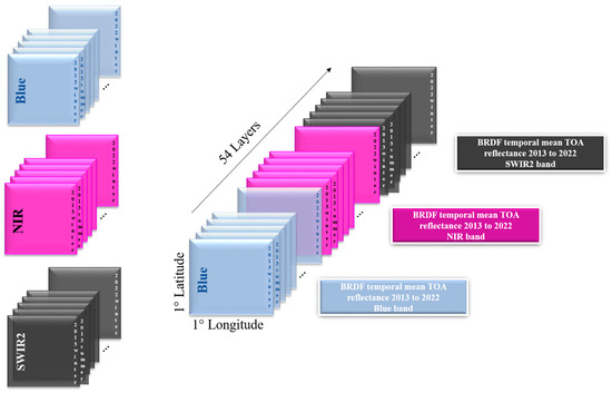
Figure 8.
Data cube structure for evaluation of temporal stability on a global scale.
Although two points represented each year, as explained earlier, the seasonal effect was still present. In order to reduce the seasonal effect, summer months were selected as the reference, and data representing the winter months were normalized to the reference reflectance for each pixel using the following equation:
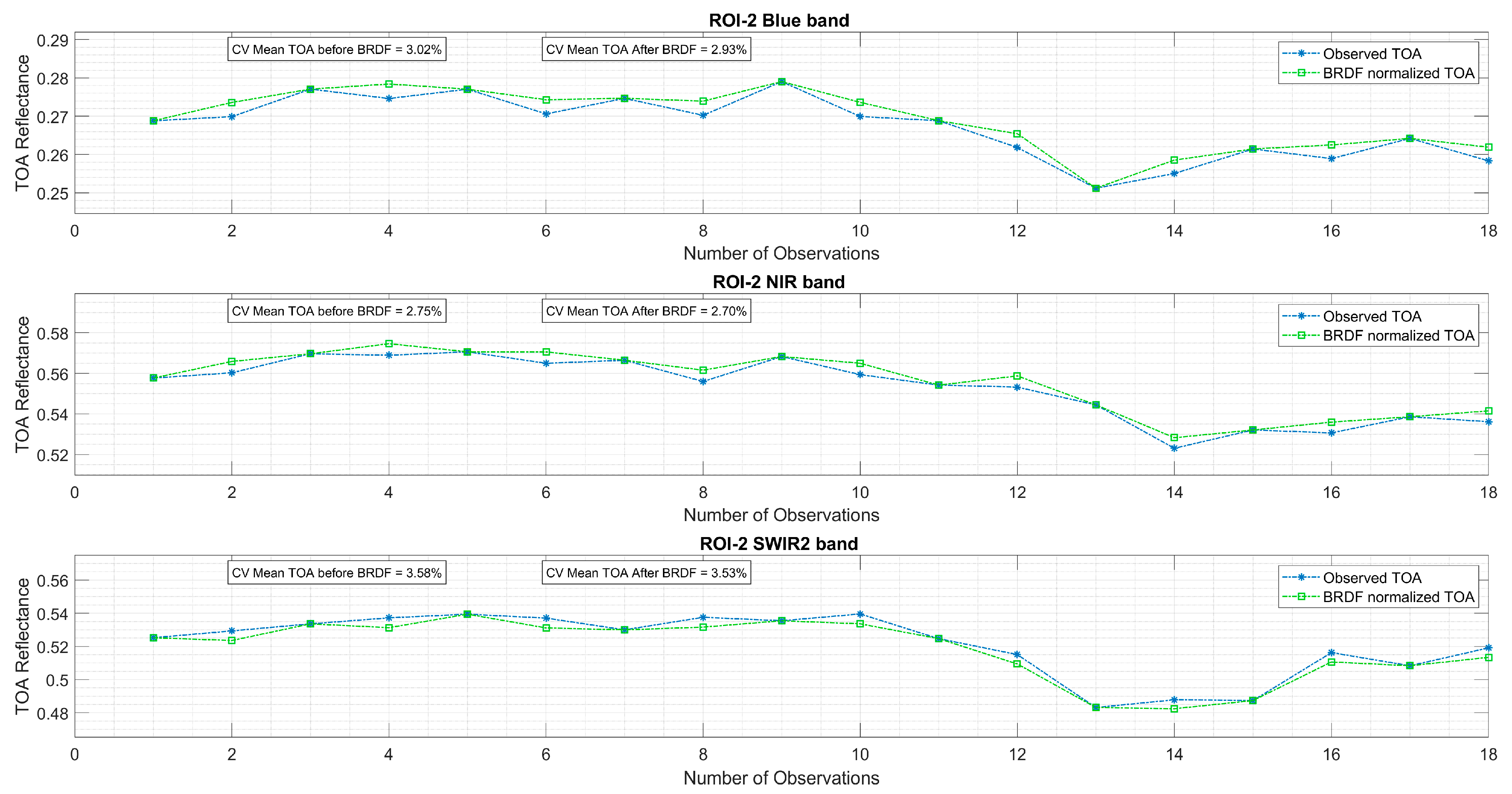
Figure 9 and Figure 10 illustrate the same pixels in the ROIs presented above but for the data cubes with 18 data points. It is evident from Figure 9 that the pixel over ROI-1 exhibited temporal stability, consistent with observations from Figure 6 where all available data were utilized. Additionally, noticeable seasonal variations in TOA reflectance between summer and winter months were observed, with normalization of winter months to summer months reducing these seasonal effects. Furthermore, Figure 10 depicts the cubes with 18 data points for ROI-2. Here, the seasonal effect was less pronounced compared with the pixel shown in Figure 9, consistent with Figure 7 where all available data were used, resulting in a less significant reduction in CV compared with the North African site. Despite the downsampling of the data, the underlying temporal variability of the pixel remained evident.
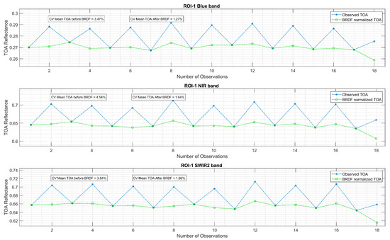
Figure 9.
Temporal mean TOA reflectance of a randomly selected pixel from ROI-1 using the data cubes containing two points per year (summer and winter).
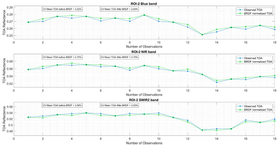
Figure 10.
Temporal mean TOA reflectance of a randomly selected pixel from ROI-2 using the data cubes containing two points per year (summer and winter).
The examples shown in Section Pixel Level BRDF Normalization Using a 4-Angle Model and in the current section demonstrate the application of BRDF in data cubes created for both stages of this study. It is important to note that certain regions or pixels exhibited varying degrees of seasonal effects, some more pronounced than others. However, the BRDF normalization techniques employed in this analysis effectively mitigated the BRDF effect. For future analyses, increasing the number of data points could enhance the ability to generate and apply BRDF model normalization, as observed in examples where all the available data in the SDSU IP LAB archive were utilized.
2.3. Statistical Test Application at the Pixel Level and Selection of Test to Obtain a Global Mosaic of Temporal Stable Pixels (Stages 1 and 2)
The choice of ROIs for this study was made to carry out two key steps toward the final goal of selecting a statistical test(s) to perform the identification of temporally stable pixels on a global scale. In both steps, the effectiveness of each test applied individually, as well as the performance of the long-term trend and change-point detection tests combined, were evaluated. The tests and combination of tests applied to each pixel time series are listed in Table 1.

Table 1.
Tests and combination of tests in evaluation.
The per-pixel application of statistical tests and combination of tests resulted in binary masks containing temporally stable pixels only (stable pixels 1, unstable pixels 0). In the application of the linear and quadratic models, a pixel was considered stable if the confidence interval of the fit contained zero, suggesting that the time series under consideration did not exhibit significant linear or quadratic behavior. In addition, for the Mann–Kendall test, Pettitt’s test, and Spearman’s rho test, a significant trend or change-point detection was identified using a 5% significance level. For CUSUM control charts, the upper and lower thresholds were determined based on a 3-sigma value estimation. The same conditions were used for the combination of long-term trend and change-point detection tests. Moreover, in the combined tests, a pixel time series was considered temporally stable only if both long-term detection and change-point detection indicated no changes over time.
As mentioned earlier, in order to select the test for identifying temporally stable pixels on a global scale, two significant steps were taken. In the first step, the performance of all tests listed above was evaluated over the testing ROIs using the data cubes containing all available Landsat 8-OLI data, as described in Section Generation of Testing Data Cubes with All Available Landsat 8-OLI Data. To evaluate the binary masks containing temporally stable pixels identified by the tests, temporal time series of 100 random pixels were visually inspected and classified as temporally stable or unstable. These results were then compared with the results of each test for each ROI. The statistical test or combination of tests that exhibited the highest agreement with the visual inspection was selected as the reference binary mask for each ROI to evaluate step 2. This mask was taken as a reference because all available data were used in the temporal stability evaluation.
The second step for this work was to evaluate the same three regions (ROI-1, ROI-2, and ROI-3) using the same statistical tests but utilizing shorter time series. Considering that the final goal of this work was to perform a global evaluation of temporal stability at the pixel level and ultimately generate a global mosaic of temporally stable pixels, the time series per pixel were reduced to two representative points per year. This step was to verify whether the results remained consistent even when employing a restricted set of input data, such as shorter time series. This was due to computational and storage capabilities at the SDSU IP LAB, as explained in Section Generating Global Data Cubes Using Google Earth Engine (GEE).
The resulting binary masks of the second step were then compared with the reference masks obtained in step 1. Since the global product created as described in Section Generating Global Data Cubes Using Google Earth Engine (GEE) has a 90 m spatial resolution, the binary masks obtained in step 2 were resampled to 30 m spatial resolution and reprojected to the Landsat 8 UTM projection system for this comparison. Given that this was a pixel-by-pixel comparison, it was necessary to be able to compare binary masks created in stages 1 and 2 at the same resolution. Resampling and reprojection were achieved using a raster and vector geospatial data converter library offered by the Open-Source Geospatial Foundation. From this data converter, called the Geospatial Data Abstraction Library (GDAL), the gdalwarp function was used [32].
In addition, the test or combination of tests with the highest agreement between binary masks obtained in step 1 and step 2 was selected as the test or combination of tests to identify all temporally stable pixels on a global scale, using the data cubes generated in Section Generating Global Data Cubes Using Google Earth Engine (GEE). Finally, the computational time for each test was also considered in the process of selecting the optimal test or combination of tests for the global temporal filter.
3. Results and Analysis
3.1. Identification of Temporally Stable Pixels Using All Available Data from Regions 1, 2, and 3
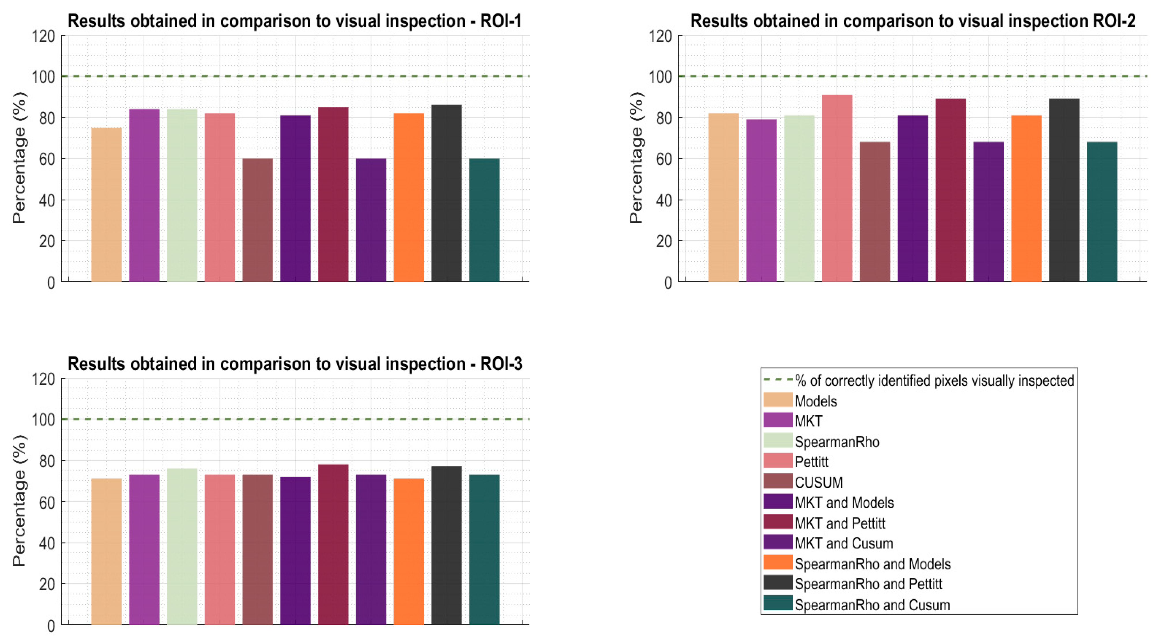
The performance of each test or combination of tests used to generate binary masks for the three ROIs was evaluated by comparing them to visually inspected samples, as described in Section 2.3. The percentage of pixels correctly classified as temporally stable or unstable was computed for each test or combination of tests based on the visually inspected samples. The results, presented in Figure 11 and Table 2, showed that the CUSUM control chart had the lowest performance across all testing sites. On the other hand, the combination of the Mann–Kendall and Pettitt’s tests and that of the Spearman’s rho and Pettitt’s tests were among the top-performing tests across all three sites.

Figure 11.
Results obtained after comparing the resulting binary mask with visual inspection of 100 randomly selected pixels. The green dashed line represents the total percentage of pixels correctly identified by visual inspection (reference percentage), and bars represent the results of the same pixels for each test.

Table 2.
Total percentage of pixels correctly identified as stable and unstable when comparing the binary mask with visual inspection of 100 randomly selected pixels.
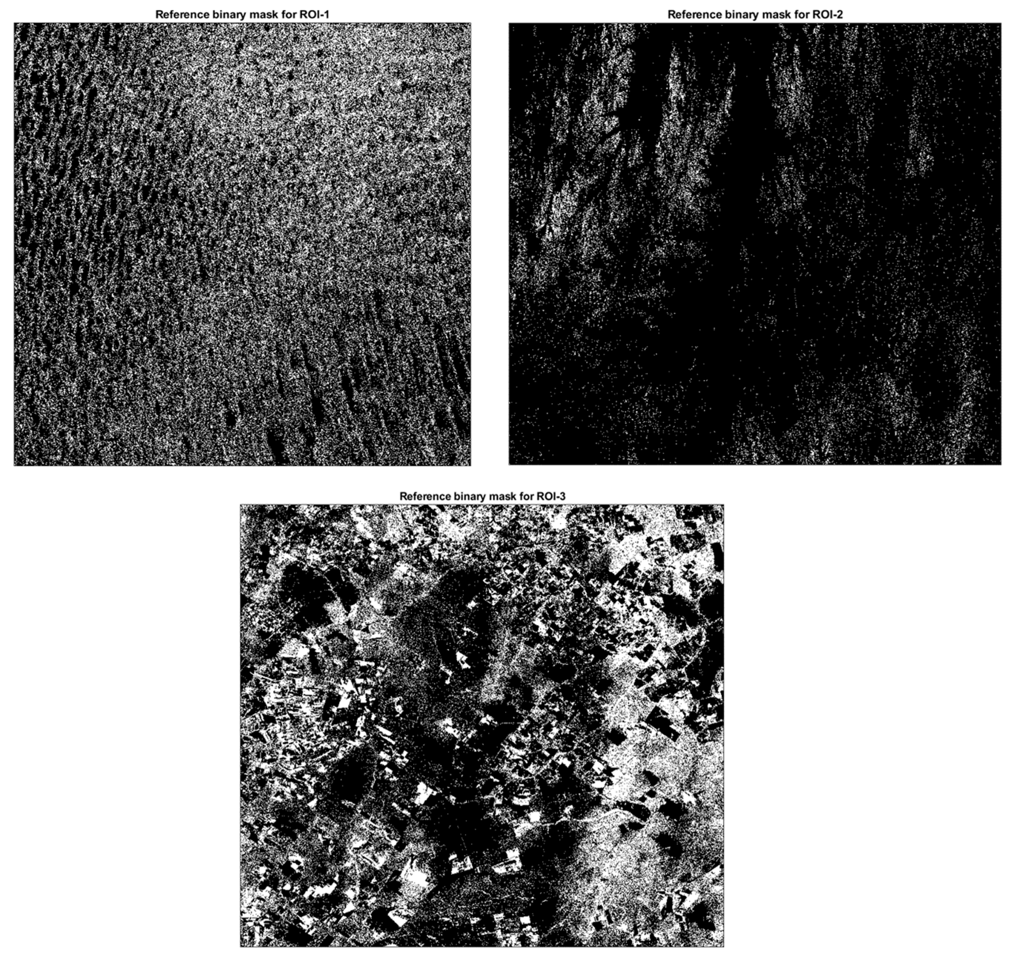
The analysis revealed that the combination of the Spearman’s rho and Pettitt’s tests consistently demonstrated results that were among the top three most accurate for all three ROIs. While the combination of the Mann–Kendall test and Pettitt’s test showed similar outcomes, the combination of the Spearman’s rho and Pettitt’s tests retained a greater number of pixels for ROI-1, where Libya 4-ROI is located, while being equally effective in removing unstable pixels from ROI-2. Hence, the binary mask derived from applying the Spearman’s rho and Pettitt’s tests was selected as the reference binary mask for step 1, as explained in Section 2.3. Figure 12 displays the reference binary masks containing temporally stable pixels identified by the combination of Spearman’s rho and Pettitt’s test, where the white regions represent the stable pixels. These masks were then taken as a reference to assess the performance of each test on the data cubes with shorter time series (18 points per pixel). Table 3 represents the percentage of temporally stable and unstable pixels in the reference binary masks for each ROI after the application of tests.

Figure 12.
Resulting binary masks obtained after the application of Spearman’s rho test and Pettitt’s test and selected as reference binary masks for the ROIs under study.

Table 3.
Percentage of temporally stable and unstable pixels in the reference binary masks for all three ROIs in this study, obtained after the application of Spearman’s rho and Pettitt’s tests on the data cubes containing all available Landsat 8-OLI data.
3.2. Selection of Statistical Test for Obtaining Temporally Stable Pixels at a Global Scale
As mentioned previously, the reference binary masks containing temporally stable pixels generated from the application of the Spearman’s rho and Pettitt’s tests to the data cubes containing all available Landsat 8-OLI data served as a benchmark for evaluating the performance of all tests on the data cubes containing only 18 data points. This evaluation aimed to select the optimal test or combination of tests for a global temporal stability analysis. To accomplish this, the binary masks generated from the tests or combinations of tests applied to the data cubes with 18 data points that showed the highest agreement with the reference binary masks were chosen in order to perform a global stability analysis. It is worth noting that this analysis was carried out with the aim of selecting the test that demonstrated the best performance when using shorter time series. The computational time for each test site was also taken into account when selecting the test or combination of tests for the global temporal filter.
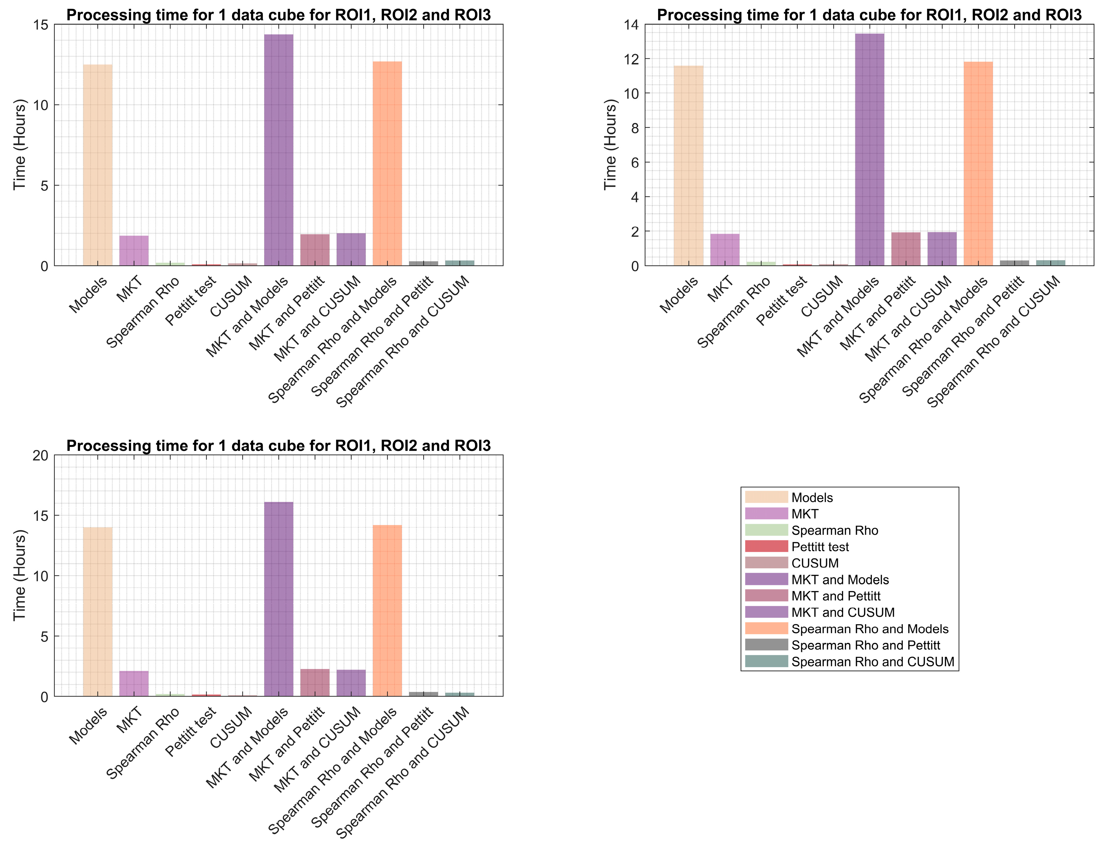
As mentioned above, to select the optimal method for identifying temporally stable pixels on a global scale, two factors were considered: accuracy and computational time. Figure 13 and Table 4 present an overview of the computational time required for each test, and the test or combination of tests with the highest accuracy and lowest computational time was selected as the optimal solution for the global analysis. The combination of the Spearman’s rho test and Pettitt’s test proved to be the most efficient, taking approximately 30 min to process each data cube. In contrast, the combination of the Mann–Kendall test and the linear and quadratic models was the least efficient, taking over 14 h to process a single data cube. Given that a total of 9258 data cubes were processed in this study, computational time was a crucial factor in the test selection.
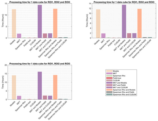
Figure 13.
Computational time taken by each statistical test to process one data cube for each ROI.

Table 4.
Computational time in hours for each test applied to one data cube (1° latitude, 1° longitude) including all three bands analyzed in this study.
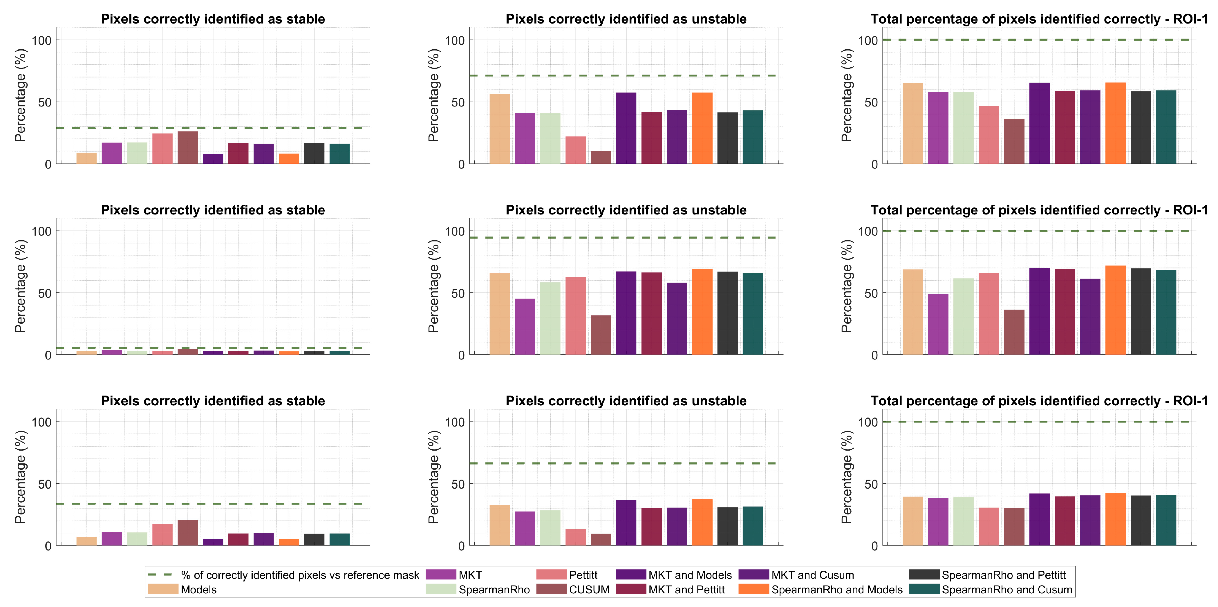
Figure 14 and Table 5 show the accurate identification of temporally stable and unstable pixels in data cubes with 18 points per pixel, compared with the reference binary mask shown in Figure 11. Across all regions, the most effective method was found to be the combination of Spearman’s rho test and the linear and quadratic model test. However, in ROI-1, a homogeneous desert region, this combination of tests identified a substantial number of pixels as temporally unstable, despite being labeled as stable in the reference binary mask. The method correctly identified only 8% of over 28% of stable pixels in that region. The Mann–Kendall test and the combination of the Mann–Kendall test and linear and quadratic models also exhibited an overly aggressive filtering of stable pixels, removing over 25% of temporally stable pixels identified as stable in the reference result.
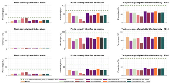
Figure 14.
Percentage of pixels correctly identified as stable and unstable in each ROI when compared with the reference binary mask. Tests were applied to data cubes containing 18 data points per pixel.

Table 5.
Percentage of pixels correctly identified as stable and unstable in each ROI when compared with the reference binary mask. Tests were applied to data cubes containing 18 data points per pixel.
The combination of Spearman’s rho test and Pettitt’s test proved to be effective in removing over 40% of temporally unstable pixels in ROI-1, which represented more than 57% of the unstable pixels in the reference result. At the same time, this method retained 17% of the temporally stable pixels in the region, which represented more than 47% of the stable pixels in the reference result. These results were similarly observed in ROI-2 and ROI-3. For example, in ROI-2, a region with known unstable pixels, the Mann–Kendall test and CUSUM control charts performed poorly in removing unstable pixels, while Pettitt’s test, Spearman’s rho test, the linear and quadratic model tests, and the combination of these tests performed better. Moreover, the study found that in some cases, the combination of a long-term trend and change-point detection techniques was more effective in accurately identifying temporally stable and unstable pixels compared with applying individual tests.
In summary, the combination of the Spearman’s rho test and Pettitt’s test emerged to as the most effective approach for identifying temporally unstable pixels while preserving a high percentage of stable pixels across all regions. Furthermore, this combination of tests displayed the highest level of computational efficiency. As a result, the combination of Spearman’s rho test and Pettitt’s test was chosen as the methodology for creating a global mosaic of temporally stable pixels.
3.3. Global Mosaic of Temporally Stable Pixel
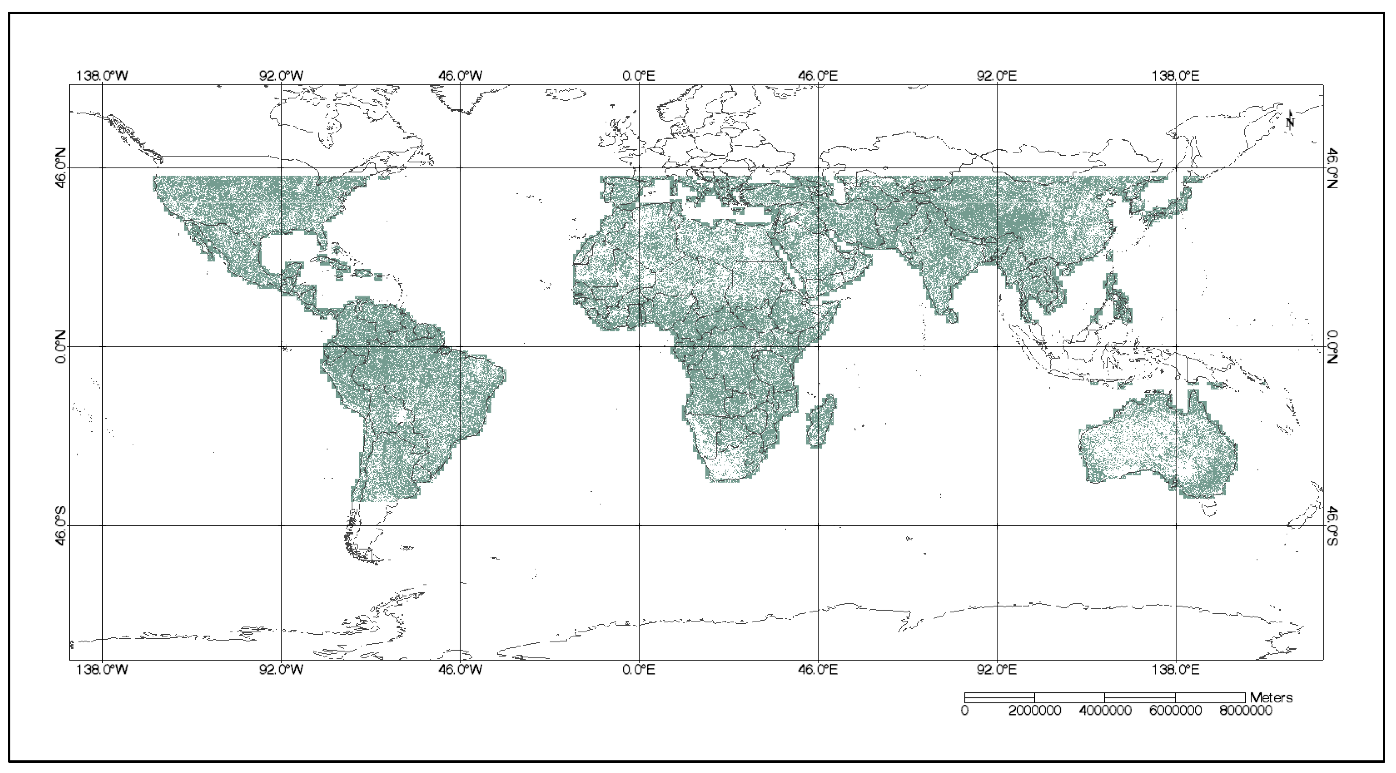
In this study, a mosaic of temporally stable pixels was generated through a per-pixel temporal evaluation using the combined approach of the Spearman’s rho test for long-term trend detection and Pettitt’s test for change-point detection. Figure 15 illustrates the resulting mosaic of 9238 binary masks, indicating temporally stable pixels identified after applying these tests to each pixel. The green pixels in the mosaic represent regions with temporal stability across the world. However, this global visualization can be deceiving, as higher contrast is evident when examining smaller areas. Depending on the region, several locations consist mostly of unstable pixels. Figure 16 provides a detailed view of WRS-2 path 179/row 76, offering improved clarity regarding pixel distribution. This closer examination highlights the detection of areas within the dunes that exhibit temporal stability as well as those showing variability. Additionally, the image demonstrates the anticipated identification of most of the ocean as temporally stable. However, it also reveals that, despite cloud filtering, traces of clouds persist in the data, suggesting that cloud masks may not completely eliminate cloud contamination. This could potentially affect the results of the analysis for some pixels.
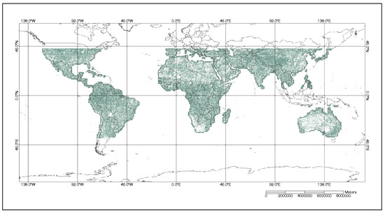
Figure 15.
Temporally stable pixels across the world (green) resulting from the application of Spearman’s rho test and Pettitt’s test for long-term trends and change-point detection.
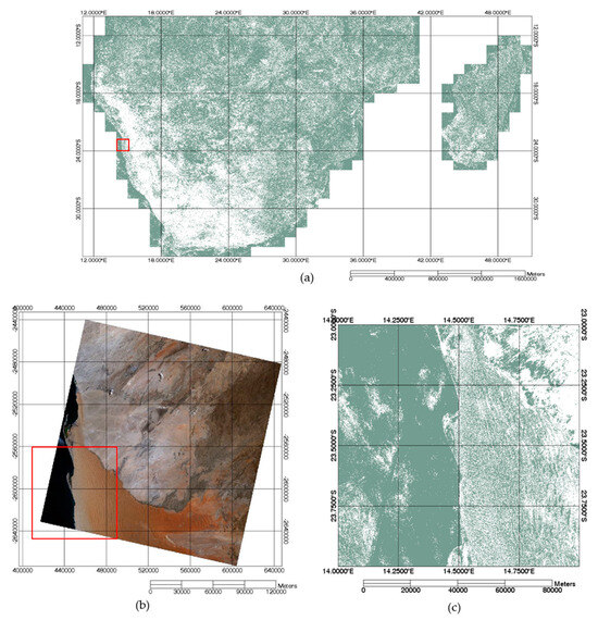
Figure 16.
Pixel distribution in the mosaic of temporally stable pixels for a region within WRS-2 path 179/row 76 in South Africa. (a) South African mosaic of temporally stable pixels, (b) WRS-2 Path/Row, (c) resulting binary mask of temporally stable pixels within the red box in (b).
These masks play a crucial role in identifying prospective regions suitable for calibration and stability monitoring of optical satellite sensors. Nevertheless, it is essential to consider that the subsampling of time series data may result in some unstable pixels with subtle variabilities remaining undetected. In future analysis resampling this study, enhanced storage capabilities could facilitate the inclusion of more data in the time series. Consequently, this would result in a more refined identification of those subtle changes, contributing to deeper understanding of temporal trends and pixel stability on a global scale.
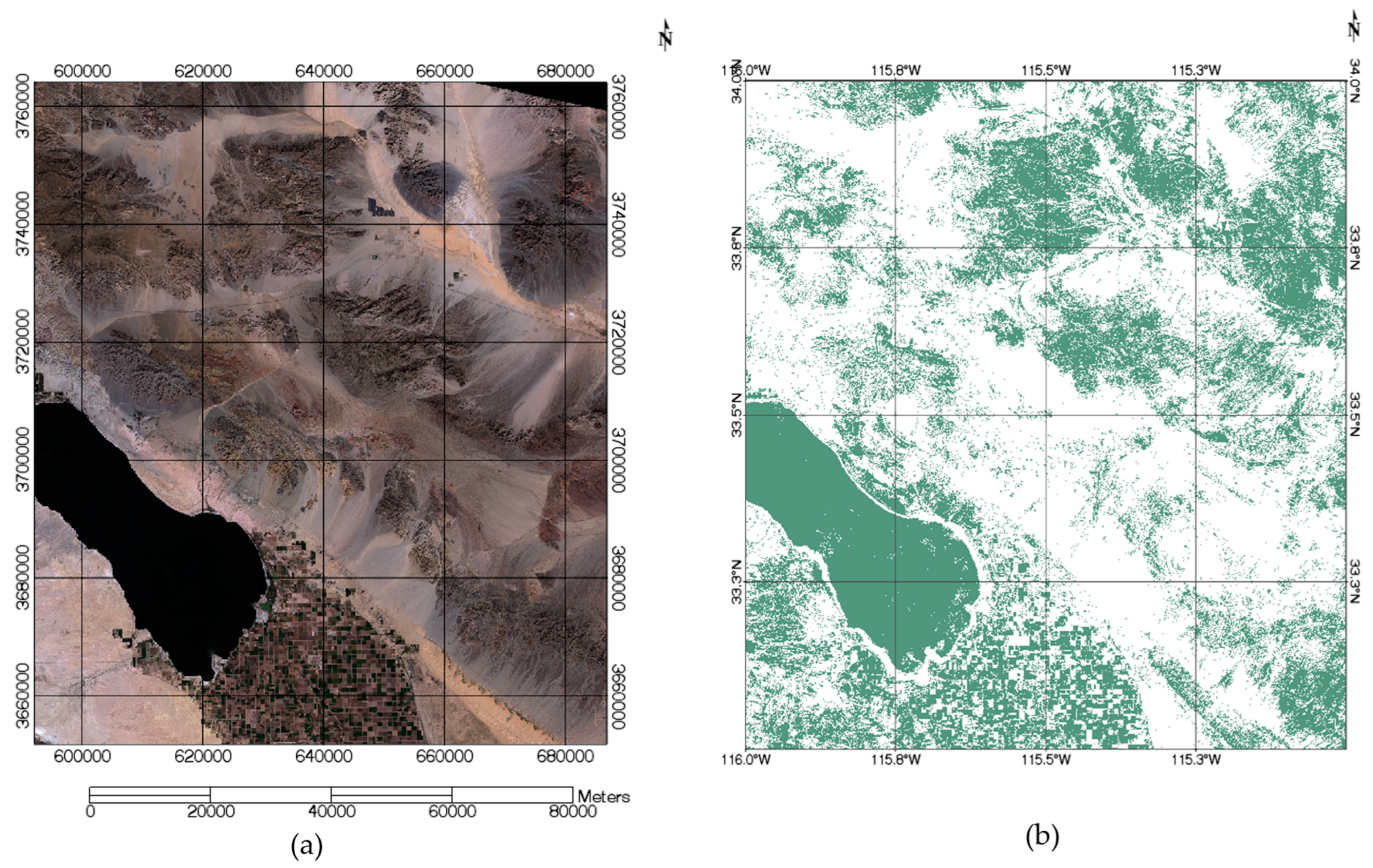
Figure 17 illustrates how various factors can influence pixel stability, presenting results from temporal pixel analysis over data cubes generated in GEE, as explained in Section 2.3. Figure 17a displays a Landsat 8 RGB image from WRS-2 path 39/row 37, while Figure 17b shows the 1-degree by 1-degree binary mask generated by applying Spearman’s rho and Pettitt’s test to the 18-layer data cube across the region during the temporal stability evaluation stage. The scene includes diverse land cover types such as crops, water bodies, rocks, and sand.
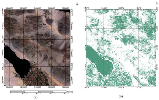
Figure 17.
(a) RGB image of WRS-2 path 39/row37 showing different land cover types such as crops, water, sand, rock formations, etc.; (b) temporal filter mask obtained in this study over the same region of part of WRS-2 path 39/row 37.
The temporal stability analysis identified the water of Salton Sea Lake as temporally stable, whereas the lake shore was identified as temporally unstable, as seen in Figure 17b. This instability may have resulted from water level changes throughout different seasons, altering pixel reflectance from dark (water) to brighter (sand/lake bed) as water levels decreased, or may potentially have been due to sediments on the lake bed shore. Large rock-covered areas were also identified as temporally stable, possibly due to their remote locations and lack of vegetation reducing susceptibility to temporal changes. Additionally, various crop areas were visible, with some identified as temporally stable and others as unstable. Differences may be linked to crop type and mean TOA reflectance changes between the summer and winter months considered in this study. Stable areas may exhibit minimal changes, while unstable areas may show more pronounced variations due to seasonal changes on the ground or the presence of different crop types. It is important to note that the spatial resolution in this study was 90 m; therefore, detecting mean TOA reflectance changes in crop areas was more challenging compared with larger areas such as sand dunes, large water bodies, and large rock formations.
These observations indicate that with only two seasons considered, subtle changes over time may go undetected. Increasing the number of data points in the time series could enhance the detection of such changes in mean TOA reflectance. Nevertheless, this example underscores the potential of this approach for identifying globally stable regions on large scales considering different cover types, providing a valuable foundation for future studies. Expanding this methodology to include data cubes with more layers could further improve the detection of more subtle temporal changes.
4. Validation
To validate the temporal binary masks obtained in this study, a specific region known to contain temporally unstable pixels was used. This region was identified by Fajardo et al. during a global clustering of pixels using an unsupervised K-means algorithm. The primary goal of the authors’ analysis was to identify regions suitable for radiometric calibration on a global scale. It is worth noting that in that work, the authors did not apply any temporal filter or perform any evaluation of per-pixel temporal stability. Among the clusters identified in that analysis, the authors selected one cluster resulting from implementing the k-means clustering algorithm that demonstrated potential to be considered a globally extended pseudo invariant calibration site (Global EPICS). These EPICSs are locations where pixels are aggregated together over a broad geographical area and exhibit similar temporal, spatial, and spectral characteristics. Consequently, EPICSs offer multiple calibration points per day, depending on the sensor’s temporal resolution.
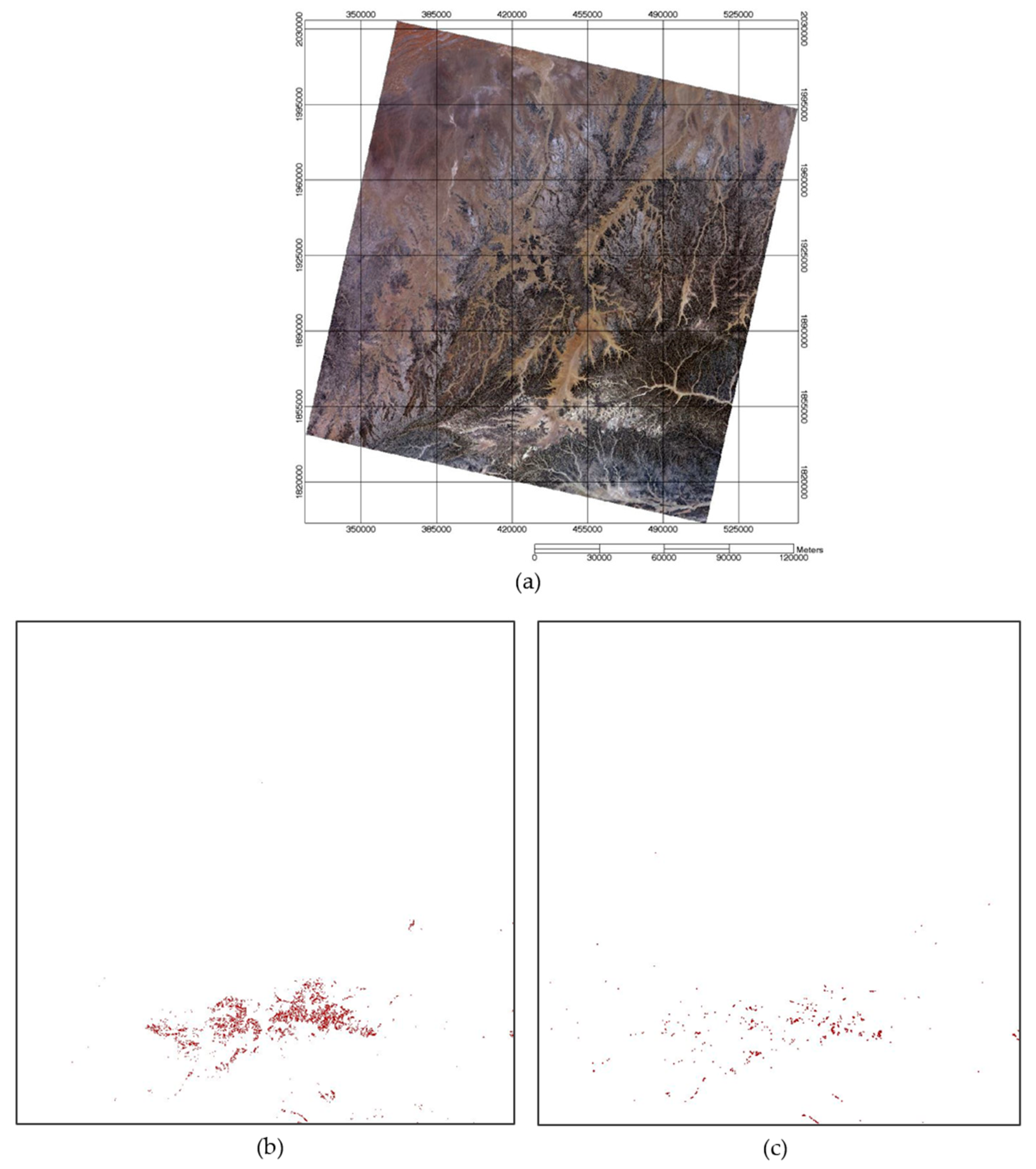
In that analysis, the potential global EPICS was named Global Cluster 13 (GC13). GC13 encompassed several locations across the world, and one of these regions was found within the WRS-2 path 162/row 48 in the Middle East. However, despite the inclusion of pixels from WRS2 path 162/row 48 in GC13, the authors had to remove these locations entirely from their analysis due to the presence of temporally unstable pixels. As stated earlier, incorporating temporally unstable pixels in the targets used for evaluation of stability monitoring can result in incorrect identification of changes in the sensor’s response. Figure 18a displays a Landsat 8-OLI image intersected with GC13 pixels, and Figure 18b presents a binary mask indicating the pixels identified as part of GC13 within WRS-2 path 162/row 48, depicted as red regions. Lastly, Figure 18c displays the binary mask of the remaining pixels after the application of the temporal filter used in this study. The validation of the temporal filter focused on excluding pixels with temporal instability was carried out via comparing the TOA reflectance of Landsat 8-OLI sensor data for GC13 pixels within WRS-2 path 162/row 48 before and after the application of the filter. The pre-filtered TOA reflectance was computed from a total of 354,053 pixels, while the post-filtered TOA reflectance was computed based on 21,945 pixels, indicating that the temporal filter application effectively removed approximately 93.8% of pixels within the GC13 region.

Figure 18.
(a) Landsat 8-OLI image of WRS-2 path 162/row 48; (b) GC13 pixels within WRS-2 path 162/row 48 before temporal filter application; (c) GC13 pixels within WRS-2 path 162/row 48 after the temporal filter application.
TOA reflectance for the pixels used in this study was obtained using the equation described in Section 2.2.2. Cloud screening was achieved using the pixel quality assessment band from the level 1 Collection 2 data, using the same bit information described in Section Filtering Process Using the Pixel Quality Assessment Band Data and following the cloud filtering methodology for GC13 used by Fajardo et al. In the referenced study, a binary mask containing clear pixels was generated and overlaid with the GC13 region, in this case, for WRS-2 path 162/row 48. If more than 50% of the pixels within GC13 over that specific region were affected by cloud contamination, the scene was excluded from further analysis due to the substantial cloud presence. For scenes with less than 50% cloud cover over the GC13 pixels, a per-pixel cloud filtering was performed utilizing the per-scene generated cloud-free binary mask.
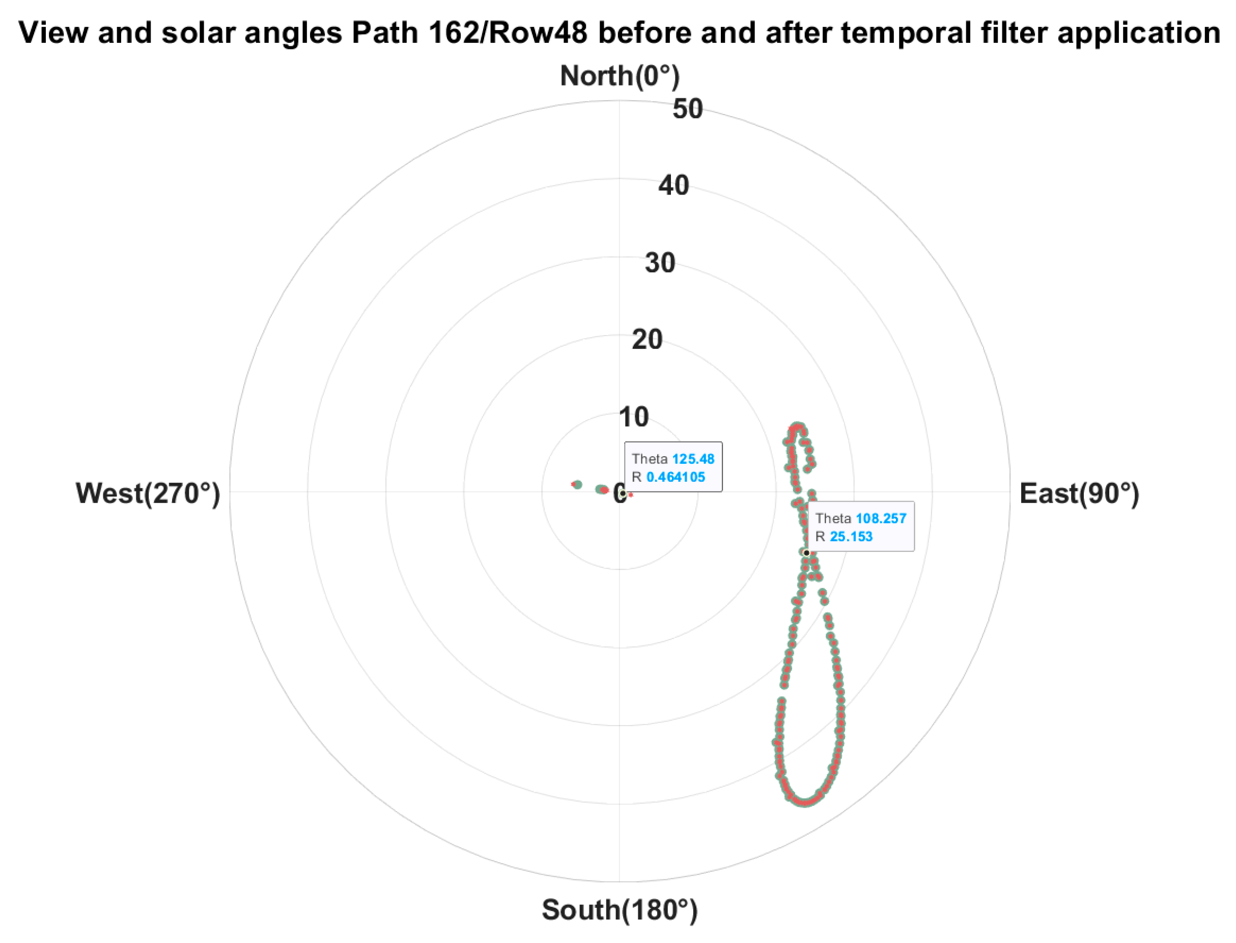
Seasonal variations in mean TOA reflectance were normalized using the BRDF model described in 2.2.2.3, which employed BRDF normalization using a four-angle model. The selection of reference angles to obtain the reference reflectance for this normalization was based on central values depicted in a polar plot (Figure 19), ensuring consistency across both datasets. The selected reference angles were solar zenith angle = 25, solar azimuth angle = 108, view zenith angle = 0.5, and view azimuth angle = 125.
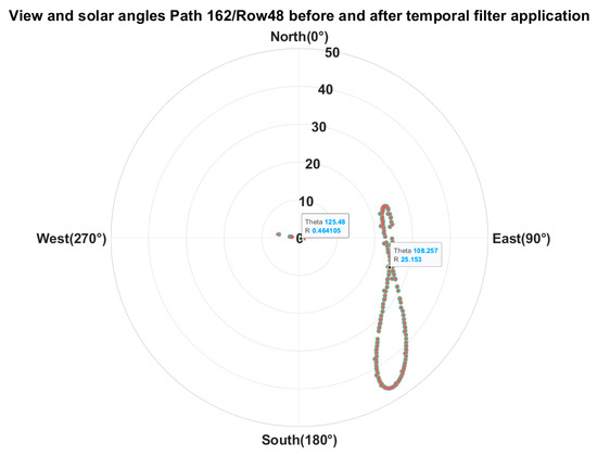
Figure 19.
Polar plot displaying reference angles to calculate reference reflectance in the BRDF model application. Red markers represent pre-filter data and green markers display post-filter data.
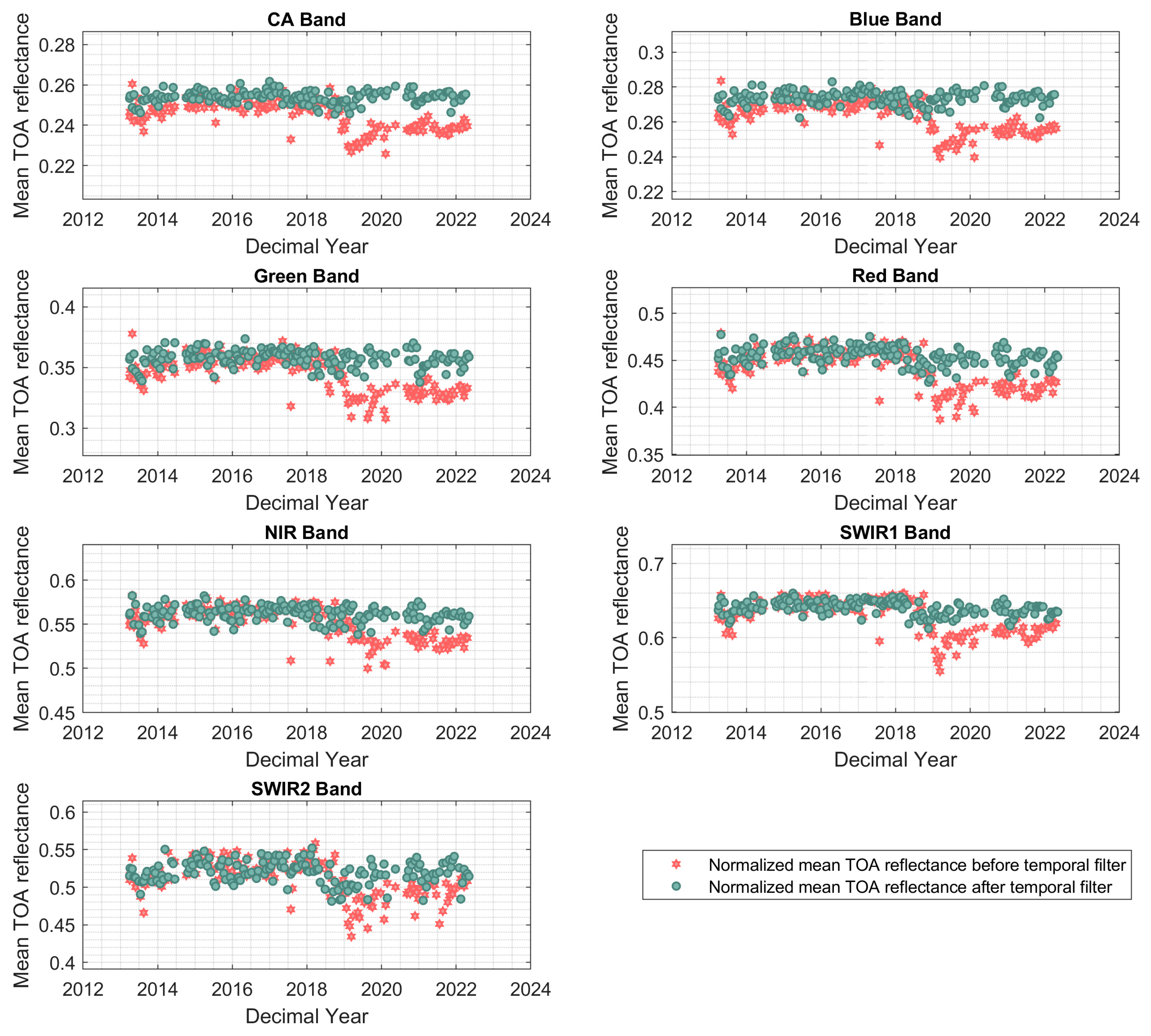
BRDF-normalized TOA reflectance before and after the temporal filter application for all Landsat 8-OLI spectral bands is shown in Figure 20. In addition, Table 6 shows temporal mean TOA reflectance, standard deviation, and CV, representing the ratio of temporal standard deviation to temporal mean TOA reflectance. It is evident from the analysis that the CV values for the pre-filtered data were consistently higher in comparison to the CV values observed in the post-filtered data set for all spectral bands.
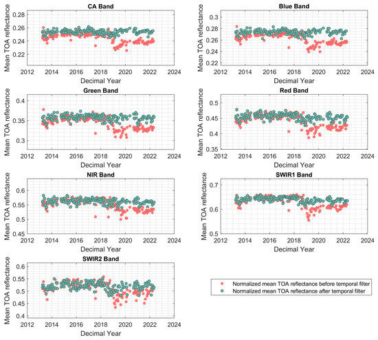
Figure 20.
Time series of TOA reflectance for GC13 pixels in WRS-2 path 162/row 48 before (red) and after (green) the temporal filter application.

Table 6.
Statistics containing temporal mean, temporal standard deviation, and CV for TOA reflectance over WRS-2 path 162/row 48 in the Middle East before and after the temporal filter application.
To further assess the changes in TOA reflectance before and after applying the temporal filter, a comparative analysis was conducted on the pre-filtered and post-filtered datasets. These datasets were divided into two distinct time frames: an initial period from 2013 to 2019, characterized by minimal temporal instability in both datasets, and a subsequent period from 2019 to 2022, when evident temporal changes occurred in the pre-filtered data. To quantify the difference in mean TOA reflectance before and after applying the temporal filter, a comparative analysis was conducted on both the pre-filtered and post-filtered datasets.
To estimate the change in temporal mean TOA reflectance before and after the temporal change, the mean of the mean TOA reflectance was computed for both time frames in both datasets. This analysis was performed separately for each band. Table 7 presents the computed differences in reflectance units, as well as the percentage change relative to the temporal mean TOA reflectance of the stable time frame (2013–2019) for both pre-filtered and post-filtered datasets. Notably, for the pre-filtered dataset, the red band exhibited the largest mean TOA reflectance difference, with an average difference of −7.5% between the TOA reflectance before and after the temporal change. Conversely, the coastal aerosol band showed the lowest difference of −4.6%. In contrast, the same analysis was performed on the post-filtered dataset, revealing considerably reduced differences. The coastal aerosol band demonstrated the lowest difference, with values as low as −0.1%. On the other hand, the red band exhibited the highest difference of only −1.6%, indicating a notable reduction of 5.9% in the TOA reflectance difference before and after the temporal change after the application of the temporal filter mask obtained in this study. This reduction suggested that the temporal filter effectively minimized the temporal variations in the post-filtered data, leading to a more stable time series.

Table 7.
TOA reflectance differences between time frame 1 (2013–2019) and time frame 2 (2019–2022) for the pre-filtered and post-filtered datasets.
To further validate the effects of the temporal filter developed in this study on the mean TOA reflectance, a statistical analysis was conducted to validate the temporal stability of the mean TOA reflectance trend derived from the study area WRS-2 path 162/row 48. This involved evaluating the significance of the slope through linear regression analysis on the temporal mean TOA reflectance for both the pre-filter and post-filter datasets.
Using the BRDF-normalized data for both the pre-filter and post-filter datasets, the temporal stability analysis was conducted. This analysis involved computing linear regression and slopes using a Monte Carlo simulation approach with 1000 iterations. This approach considered not only the mean TOA reflectance but also the associated uncertainties of each measurement. The Monte Carlo method is an algorithmic approach that uses random sampling techniques and iterative processes to approximate results. It involves generating random numbers that correspond to the probability density functions (PDFs) of the primary quantities considered [33]. In the analysis, these random values are then propagated through a mathematical measurement model based on linear regression. The linear fit implemented in this study used a weighted linear regression to determine optimal parameters for a linear model that best fitted the dataset while considering uncertainties associated with each data point [34].
For uncertainty estimation, the guide to the expression of uncertainty in measurement (GUM) methodology was followed, and three sources of uncertainty were considered [35]. The total uncertainty is shown in Equation (25). For this analysis, , was considered as the temporal CV (%) that inherently included the temporal and spatial variability of the site. In addition, was the BRDF uncertainty, considered as the RMSE measuring the differences between the observed TOA reflectance and the predicted TOA reflectance of the BRDF model. Finally, was the sensor’s uncertainty considered as the absolute radiometric calibration uncertainty of 3% for Landsat 8 [36].
Subsequently, after obtaining the slopes (β1 in Equations (26) and (27)) and their uncertainties for each spectral band through the Monte Carlo simulation, the statistical significance of these slopes was evaluated using a two-tailed t-test, with hypotheses defined as follows:
In the two-tailed test, the null hypothesis () assumes there is no significant linear relationship between x and y, while the alternative hypothesis () assumes there is a significant linear relationship between x and y. If the p-value exceeds the significance level chosen for this study, set at 0.05, the null hypothesis is not rejected, indicating insufficient evidence to conclude a significant linear relationship in the mean TOA reflectance [34].
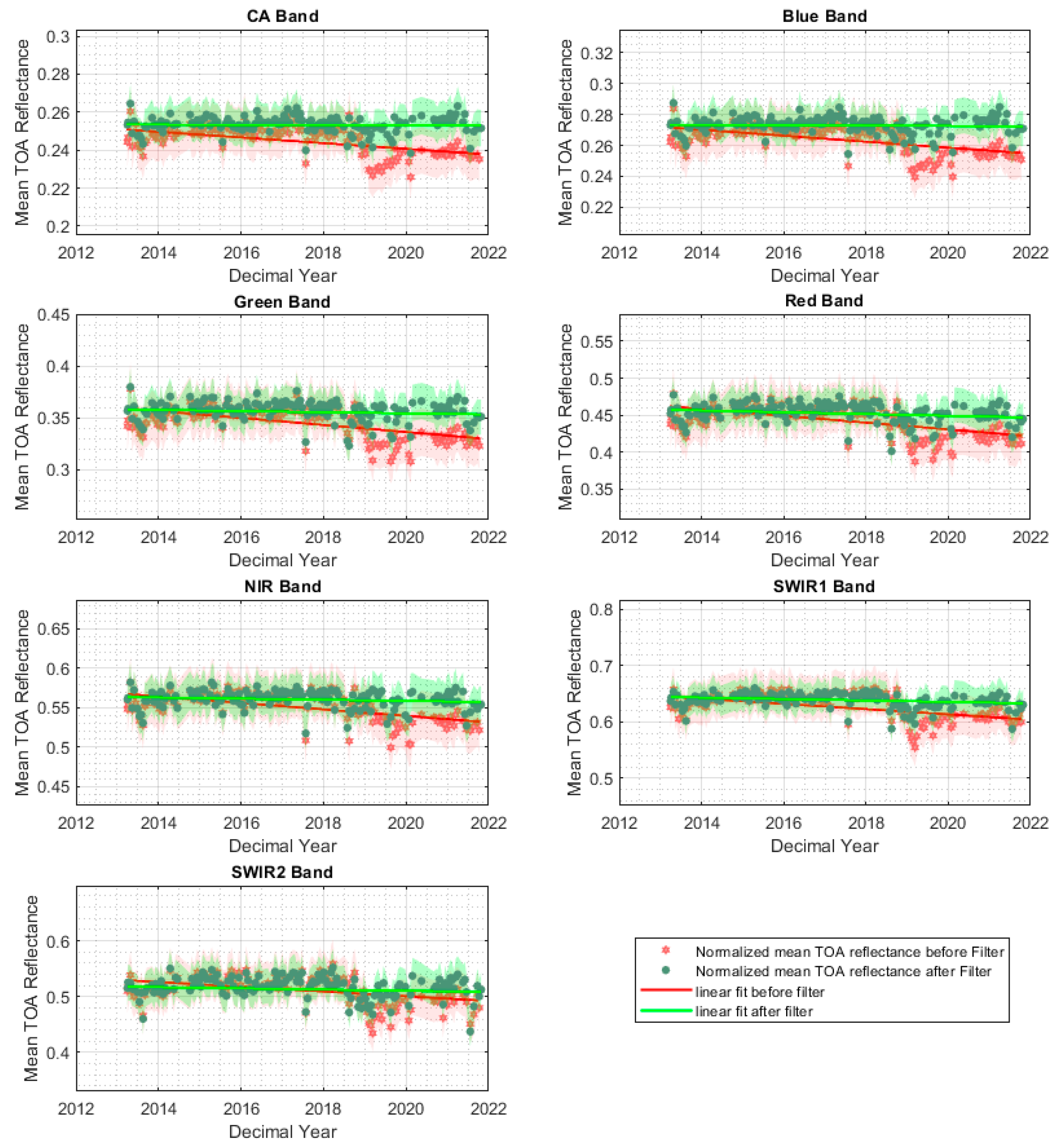
Figure 21 shows the mean TOA reflectance for the pre-filter and post-filter data, with their corresponding uncertainties displayed as the shaded area. Table 8 shows the sources of uncertainty considered for this study as well as the total uncertainty. It was noted that the application of the temporal filter developed in this study had a substantial impact in reducing uncertainties across all spectral bands, as seen from decreases in CV, BRDF, and total uncertainty. Before the filter, CV values ranged from 2.9% to 4.9%, BRDF from 3.0% to 5.1%, and total uncertainty from 5.1% to 7.6%, with the SWIR2 band consistently showing the highest uncertainties. After applying the filter, CV values decreased to a range of 1.7% to 3.6%, BRDF values reduced to approximately 1.7% to 3.9%, and total uncertainty fell to approximately 3.8% to 6.1%. Overall, CV underwent a reduction of between 1.2% to 1.9%, BRDF values were reduced by 1.3% to 2.0%, and total uncertainty by 3.3% to 4.4%. The most substantial improvements were observed in the red band for CV (1.7%), BRDF (2.0%), and total uncertainty (4.4%). These findings highlight the filter’s effectiveness in improving data reliability by removing temporally unstable pixels.
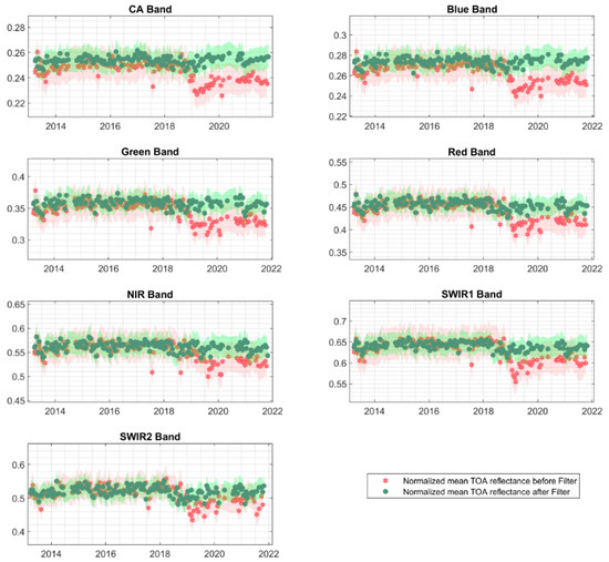
Figure 21.
Temporal mean TOA reflectance over the region of interest in path 162/row 48 using L8-OLI. Red data represent post-filter mean TOA reflectance and green data represent post-filter mean TOA reflectance. Shaded areas are the per-point uncertainty.

Table 8.
Before and after temporal filtering: (CV), BRDF, sensor’s absolute uncertainty, and total uncertainty (%).
In addition, the improvements in temporal stability after application of the temporal filter can be seen in Figure 22 and Table 9. Figure 22 shows the mean TOA reflectance before and after filtering and the corresponding slope output of the Monte Carlo simulation. Table 9 shows the slopes and p-values obtained from the application of the two-tailed t-test. It can be seen that the application of the temporal filter developed in this work resulted in significant changes in the observed trends across all spectral bands. Before filtering, negative slopes were present in all bands, indicating a decreasing trend over time. These slopes ranged from −0.002 to −0.005. However, after applying the temporal filter, the slopes for most bands became zero or near-zero, suggesting that the temporal filter effectively removed the temporally unstable pixels, as a result generating a downward trend in the mean TOA reflectance. Furthermore, the p-values before filtering were below 0.05, showing that the slopes were statistically significant. After filtering, the p-values increased substantially, with all values well above 0.05, indicating that the slopes were no longer statistically significant. This suggests that the temporal filter effectively removed any pixels with significant temporal trends in the data, resulting in a more stable dataset with no significant trends over time.
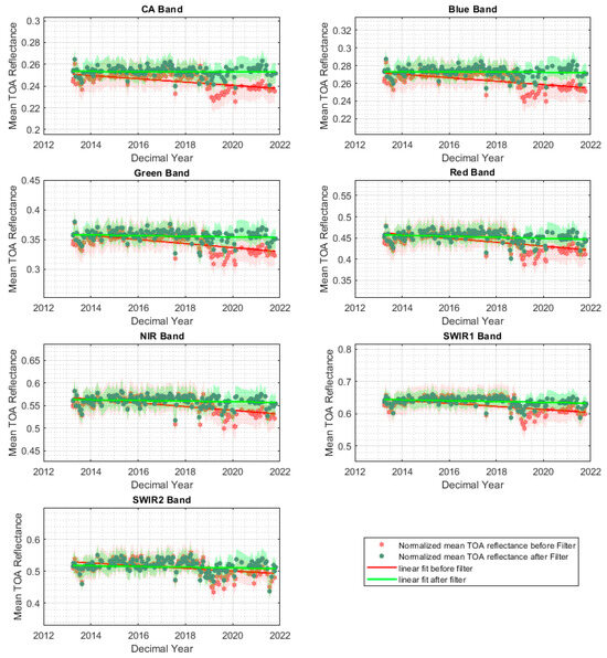
Figure 22.
Temporal mean TOA reflectance over the region of interest in path 162/row 48 using L8-OLI. Red data represent post-filter mean TOA reflectance and green data represent post-filter mean TOA reflectance. Shaded areas represent per-point uncertainty. Red and green lines represent the pre-filter and post-filter slope, respectively.

Table 9.
Effects of temporal filtering on slope, uncertainty of slope, and p-values for all spectral bands.
The temporal filter methodology and global mosaic of stable pixels presented in this study serve as a foundation for identifying potential calibration targets worldwide based on their temporal stability. The mosaic, as shown above, effectively filters temporally unstable pixels and includes only regions that have passed the temporal stability evaluation. Additionally, the developed temporal filter masks can be useful to simplify the input dataset for regional and global land cover classifications. For example, previous studies, such as Fajardo et al. [29], used k-means clustering for global land cover classification but faced challenges due to unstable pixels within clusters. Integrating these masks could enhance such classifications by ensuring that only stable pixels are classified, eliminating the need for separate evaluations of temporal stability for each pixel or region within a cluster. Furthermore, the methodology for identifying temporally stable pixels in this study can serve as a baseline for evaluating temporal stability in regional-scale targets and conducting more extensive assessments with datasets that have richer temporal data. In addition to the potential for future applications of the methodology developed in this study, the mosaic of temporally stable pixels developed here can also be used, for instance, as a pre-filter for such analyses, focusing exclusively on pixels identified as stable within this study’s scope. This approach could accelerate processing and reduce the computational resources required for evaluating each pixel individually at a regional or global scale.
In terms of radiometric calibration and stability monitoring, this study contributes to evaluating the temporal stability of on-orbit sensors and performing radiometric calibration of optical sensors. For any vicarious calibration technique requiring stable pixels, the map developed here can help refine pixel selection in existing and new ROIs used for vicarious calibration efforts, ensuring long-term stability. This refinement enhances stability monitoring and sensor calibration accuracy, considering that, as demonstrated, uncertainties between the pre-filter and post-filter data are reduced, while the validated map facilitates the identification of potential global calibration targets, expanding efforts to new geographic areas. By applying these findings, new calibration sites can be explored and established, broadening the application of sensor calibration methodologies.
In summary, this study represents a significant advancement in identifying globally stable pixels critical for radiometric calibration and stability monitoring of optical satellite sensors. Leveraging these stable regions will not only enhance current sensor calibration techniques but also provide a foundation for identifying future targets and improving global stability monitoring and calibration techniques for optical sensors.
5. Conclusions
This study aimed to assess pixel-level temporal stability globally, using Landsat 8-OLI data for the purpose of identifying regions suitable for worldwide radiometric calibration. The process involved creating data cubes, each covering a 1° by 1° grid from −43 to 43 degrees latitude and −180 to 180 degrees longitude. These data cubes consisted of 18 layers per band, representing both summer and winter data from 2013 to 2022, generated using Google Earth Engine.
To achieve this global mosaic of temporally stable pixels, a two-stage approach was implemented. Initially, this study focused on identifying effective statistical tests or combinations of tests to distinguish stable and unstable pixels using all available Landsat 8-OLI data from three diverse regions: the Middle East, North Africa, and Brazil. Six different tests were assessed: linear regression, Spearman’s rho test, the Mann–Kendall test, Pettitt’s test, quadratic model fitting, and cumulative sum control charts for their performance in assessing long-term trends and detecting change points. These tests were applied to every pixel and compared with visually inspected random samples.
A combination of tests that demonstrated the highest agreement with the visually inspected pixels served as the reference for the second stage. In this stage, the same tests were applied to the entire dataset, which included 18 data points per pixel. The comparison revealed that the combination of Spearman’s rho and Pettitt’s test achieved the highest agreement with the reference obtained in the first stage, and this was selected for the global evaluation analyses.
This analysis revealed the successful removal of the temporally unstable pixels, through comparing the mean TOA reflectance before and after implementing the temporal filter within known temporally unstable pixels. A comparative analysis was performed to evaluate changes in TOA reflectance before and after applying a temporal filter to datasets between 2013 and 2019, with stable temporal conditions, and 2019–2022, with notable temporal changes in the pre-filtered data. The analysis revealed substantial differences in TOA reflectance. For instance, in the pre-filtered dataset, the red band showed a large decrease of 7.5% in reflectance between the two time frames, while the coastal aerosol band exhibited a smaller decrease of 4.6%. Post-filtering, the differences were substantially reduced, with the red band’s reflectance decreasing by only 1.6%, and the coastal aerosol band by 0.1%. These findings highlight the effectiveness of the temporal filter in reducing variations, resulting in a more stable reflectance measurement across different time frames.
Furthermore, linear regression analysis revealed that statistically significant slopes observed in the validation study area prior to applying the filter, ranging between −0.002 and −0.005, were reduced to near zero and became statistically insignificant after applying the temporal filter. This underscored the effectiveness of the temporal filter in eliminating temporally unstable pixels. Additionally, the validation process indicated a reduction in total uncertainties between the pre-filter and post-filter data of approximately 3 to 4%, with the most significant reduction observed in the red band.
The map of temporally stable pixels developed in this work can serve as a pre-filter for land cover classification, enabling the classification of only those pixels that exhibit temporal stability. Furthermore, the methodology developed here can be expanded to datasets with richer temporal information, for regional and global-scale analysis. It was also noted that subsampling time series data might cause some unstable pixels with subtle variabilities to go undetected. For future analyses, having more data points per pixel could result in further improved results. Nonetheless, this extensive global study revealed previously undiscovered regions displaying potential for calibration and monitoring of optical satellite sensors.
Finally, the work presented in this study can serve as a valuable tool to improve vicarious calibration techniques and stability monitoring. As shown in this study, uncertainties of the targets used for such analysis were reduced after implementing this filter, allowing better stability monitoring and calibration estimates. Additionally, the global mosaic of temporally stable pixels can pinpoint new locations that can be utilized for future calibration and stability monitoring efforts. This represents a significant step forward in the search for additional calibration sites, advancing satellite sensor calibration.
Author Contributions
Conceptualization, J.F.R. and L.L.; formal analysis, J.F.R., L.L. and C.T.P.; methodology, J.F.R., L.L. and C.T.P.; software, J.F.R. and L.L.; validation, J.F.R. and C.T.P.; visualization, J.F.R.; writing—original draft, J.F.R.; writing—review and editing, L.L. and C.T.P. All authors have read and agreed to the published version of the manuscript.
Funding
This research was funded by USGS EROS (grant number G18AS00001).
Data Availability Statement
Landsat-8 image courtesy of the U.S. Geological Survey, Google Earth Engine.
Acknowledgments
The authors would like to thank the reviewers for their valuable input, the Image Processing Laboratory for the support, and David Aaron for editing the manuscript.
Conflicts of Interest
The authors declare no conflicts of interest.
References
- Liu, Y.-K.; Ma, L.-L.; Wang, N.; Qian, Y.-G.; Zhao, Y.-G.; Qiu, S.; Gao, C.-X.; Long, X.-X.; Li, C.-R. On-orbit radiometric calibration of the optical sensors on-board SuperView-1 satellite using three independent methods. Opt. Express 2020, 28, 11085–11105. [Google Scholar] [CrossRef] [PubMed]
- Helder, D.L.; Karki, S.; Bhatt, R.; Micijevic, E.; Aaron, D.; Jasinski, B. Radiometric calibration of the Landsat MSS sensor series. IEEE Trans. Geosci. Remote Sens. 2011, 50, 2380–2399. [Google Scholar] [CrossRef]
- Pinto, C.T.; Haque, M.O.; Micijevic, E.; Helder, D.L. Landsats 1–5 Multispectral Scanner System Sensors Radiometric Calibration Update. IEEE Trans. Geosci. Remote Sens. 2019, 57, 7378–7394. [Google Scholar] [CrossRef]
- Gross, G.; Helder, D.; Begeman, C.; Leigh, L.; Kaewmanee, M.; Shah, R. Initial Cross-Calibration of Landsat 8 and Landsat 9 Using the simultaneous underfly event. Remote Sens. 2022, 14, 2418. [Google Scholar] [CrossRef]
- Vogelmann, J.E.; Helder, D.; Morfitt, R.; Choate, M.J.; Merchant, J.W.; Bulley, H. Effects of Landsat 5 Thematic Mapper and Landsat 7 Enhanced Thematic Mapper Plus radiometric and geometric calibrations and corrections on landscape characterization. Remote Sens. Environ. 2001, 78, 55–70. [Google Scholar] [CrossRef]
- Chander, G.; Xiong, X.J.; Choi, T.J.; Angal, A. Monitoring on-orbit calibration stability of the Terra MODIS and Landsat 7 ETM+ sensors using pseudo-invariant test sites. Remote Sens. Environ. 2010, 114, 925–939. [Google Scholar] [CrossRef]
- Lacherade, S.; Fougnie, B.; Henry, P.; Gamet, P. Cross calibration over desert sites: Description, methodology, and operational implementation. IEEE Trans. Geosci. Remote Sens. 2013, 51, 1098–1113. [Google Scholar] [CrossRef]
- Mishra, N.; Helder, D.; Angal, A.; Choi, J.; Xiong, X. Absolute calibration of optical satellite sensors using Libya 4 pseudo invariant calibration site. Remote Sens. 2014, 6, 1327–1346. [Google Scholar] [CrossRef]
- Helder, D.; Thome, K.J.; Mishra, N.; Chander, G.; Xiong, X.; Angal, A.; Choi, T. Absolute radiometric calibration of Landsat using a pseudo invariant calibration site. IEEE Trans. Geosci. Remote Sens. 2013, 51, 1360–1369. [Google Scholar] [CrossRef]
- Cosnefroy, H.; Leroy, M.; Briottet, X. Selection and characterization of Saharan and Arabian desert sites for the calibration of optical satellite sensors. Remote Sens. Environ. 1996, 58, 101–114. [Google Scholar] [CrossRef]
- Helder, D.L.; Basnet, B.; Morstad, D.L. Optimized identification of worldwide radiometric pseudo-invariant calibration sites. Can. J. Remote Sens. 2010, 36, 527–539. [Google Scholar] [CrossRef]
- Tuli, F.T.Z.; Pinto, C.T.; Angal, A.; Xiong, X.; Helder, D. New approach for temporal stability evaluation of pseudo-invariant calibration sites (PICS). Remote Sens. 2019, 11, 1502. [Google Scholar] [CrossRef]
- Khadka, N.; Teixeira Pinto, C.; Leigh, L. Detection of change points in pseudo-invariant calibration sites time series using multi-sensor satellite imagery. Remote Sens. 2021, 13, 2079. [Google Scholar] [CrossRef]
- Qiao, E.; Ma, C.; Zhang, H.; Cui, Z.; Zhang, C. Evaluation of Temporal Stability in Radiometric Calibration Network Sites Using Multi-Source Satellite Data and Continuous In Situ Measurements. Remote Sens. 2023, 15, 2639. [Google Scholar] [CrossRef]
- Lin, T.-H.; Hsiao, M.-C.; Chan, H.-P.; Tsai, F. A Novel Approach to Relative Radiometric Calibration on Spatial and Temporal Variations for FORMOSAT-5 RSI Imagery. Sensors 2018, 18, 1996. [Google Scholar] [CrossRef] [PubMed]
- Longobardi, A.; Villani, P. Trend analysis of annual and seasonal rainfall time series in the Mediterranean area. Int. J. Climatol. 2010, 30, 1538–1546. [Google Scholar] [CrossRef]
- Chakraborty, D.; Sehgal, V.K.; Dhakar, R.; Das, D.K.; Sahoo, R.N. Trends and change-point in satellite derived phenology parameters in major wheat growing regions of North India during the last three decades. J. Indian Soc. Remote Sens. 2018, 46, 59–68. [Google Scholar] [CrossRef]
- Neeti, N.; Eastman, J.R. A contextual Mann–Kendall approach for the assessment of trend significance in image time series. Trans. GIS 2011, 15, 599–611. [Google Scholar] [CrossRef]
- Guo, M.; Li, J.; He, H.; Xu, J.; Jin, Y. Detecting global vegetation changes using mann-kendal (MK) trend test for 1982–2015 time period. Chin. Geogr. Sci. 2018, 28, 907–919. [Google Scholar] [CrossRef]
- Rahman, M.A.; Lou, Y.; Sultana, N. Analysis and prediction of rainfall trends over Bangladesh using Mann–Kendall, Spearman’s rho tests and ARIMA model. Meteorol. Atmos. Phys. 2017, 129, 409–424. [Google Scholar] [CrossRef]
- Jaiswal, R.; Lohani, A.; Tiwari, H. Statistical analysis for change detection and trend assessment in climatological parameters. Environ. Process. 2015, 2, 729–749. [Google Scholar] [CrossRef]
- Patino, C.M.; Ferreira, J.C. Confidence intervals: A useful statistical tool to estimate effect sizes in the real world. J. Bras. De Pneumol. 2015, 41, 565–566. [Google Scholar] [CrossRef] [PubMed]
- Sim, J.; Reid, N. Statistical inference by confidence intervals: Issues of interpretation and utilization. Phys. Ther. 1999, 79, 186–195. [Google Scholar] [CrossRef] [PubMed]
- Pohlert, T. Non-parametric trend tests and change-point detection. CC BY-ND 2016, 4, 1–18. [Google Scholar]
- Kale, S. Climatic trends in the temperature of Çanakkale city, Turkey. Nat. Eng. Sci. 2017, 2, 14–27. [Google Scholar] [CrossRef]
- Manogaran, G.; Lopez, D. Spatial cumulative sum algorithm with big data analytics for climate change detection. Comput. Electr. Eng. 2018, 65, 207–221. [Google Scholar] [CrossRef]
- Haq, A.; Brown, J.; Moltchanova, E. Improved fast initial response features for exponentially weighted moving average and cumulative sum control charts. Qual. Reliab. Eng. Int. 2014, 30, 697–710. [Google Scholar] [CrossRef]
- Ruiz-Ramos, J.; Marino, A.; Boardman, C.; Suarez, J. Continuous forest monitoring using cumulative sums of sentinel-1 timeseries. Remote Sens. 2020, 12, 3061. [Google Scholar] [CrossRef]
- Fajardo Rueda, J.; Leigh, L.; Teixeira Pinto, C.; Kaewmanee, M.; Helder, D. Classification and Evaluation of Extended PICS (EPICS) on a Global Scale for Calibration and Stability Monitoring of Optical Satellite Sensors. Remote Sens. 2021, 13, 3350. [Google Scholar] [CrossRef]
- Kaewmanee, M. Pseudo Invariant Calibration sites: PICS Evolution. 2018. Available online: https://digitalcommons.usu.edu/cgi/viewcontent.cgi?article=1296&context=calcon (accessed on 1 January 2023).
- Gorelick, N.; Hancher, M.; Dixon, M.; Ilyushchenko, S.; Thau, D.; Moore, R. Google Earth Engine: Planetary-scale geospatial analysis for everyone. Remote Sens. Environ. 2017, 202, 18–27. [Google Scholar] [CrossRef]
- Warmerdam, F.; Rouault, E. GDAL Documentation. Available online: http://www.gdal.org/ (accessed on 1 February 2023).
- Pinto, C.T. Uncertainty Evaluation for In-Flight Radiometric Calibration of Earth Observation Sensors; Instituto Nacional de Pesquisas Espaciais (INPE): San Jose Dos Campos, Brazil, 2016. [Google Scholar]
- Freund, R.J.; Wilson, W.J. Statistical Methods; Elsevier: Amsterdam, The Netherlands, 2003. [Google Scholar]
- JCGM. Guide to the Expression of Uncertainty in Measurement; Aenor: Madrid, Spain, 2008. [Google Scholar]
- Markham, B.; Barsi, J.; Kvaran, G.; Ong, L.; Kaita, E.; Biggar, S.; Czapla-Myers, J.; Mishra, N.; Helder, D. Landsat-8 operational land imager radiometric calibration and stability. Remote Sens. 2014, 6, 12275–12308. [Google Scholar] [CrossRef]
Disclaimer/Publisher’s Note: The statements, opinions and data contained in all publications are solely those of the individual author(s) and contributor(s) and not of MDPI and/or the editor(s). MDPI and/or the editor(s) disclaim responsibility for any injury to people or property resulting from any ideas, methods, instructions or products referred to in the content. |
© 2024 by the authors. Licensee MDPI, Basel, Switzerland. This article is an open access article distributed under the terms and conditions of the Creative Commons Attribution (CC BY) license (https://creativecommons.org/licenses/by/4.0/).

