Abstract
Ensemble Kalman filters are an efficient class of algorithms for large-scale ensemble data assimilation, but their performance is limited by their underlying Gaussian approximation. A two-step framework for ensemble data assimilation allows this approximation to be relaxed: The first step updates the ensemble in observation space, while the second step regresses the observation state update back to the state variables. This paper develops a new quantile-conserving ensemble filter based on kernel-density estimation and quadrature for the scalar first step of the two-step framework. It is shown to perform well in idealized non-Gaussian problems, as well as in an idealized model of assimilating observations of sea-ice concentration.
1. Introduction
Data assimilation combines observations, both in situ and remotely sensed, with a forecast model to estimate the state of a dynamical system. Ensemble Kalman Filters (EnKFs; [1,2]) are a class of ensemble data-assimilation methods that are widely used in large-scale Earth science applications. Ensemble filters operate sequentially in time: Each time observations become available, the ensemble forecast is adjusted, and the resulting analysis ensemble is then forecasted for the next time observations become available. The accuracy of EnKFs is limited (inter alia) by their underlying assumption of joint Gaussianity, and there is a wide range of approaches to relaxing or removing this assumption. The class of non-Gaussian extensions of the EnKF that is of interest here derives from the two-step algorithm for implementing an EnKF developed by Anderson [3]. In the first step, an EnKF is used to update an ensemble of forecast observations; in the second step, the ensemble of observation increments is converted to an ensemble of state-variable increments using linear regression. Both steps can be generalized, leading to non-Gaussian (i.e., non-Kalman) ensemble filters [4].
The focus here is on developing a nonparametric, non-Gaussian ensemble filter for the first step of this two-step process, where we assume that the first step (the update in observation space) is a scalar Bayesian estimation problem. The restriction to scalar problems is not very restrictive in light of the well-known property of Bayesian estimation that observations with independent errors can be assimilated serially in any order; the problem of assimilating many observations can, therefore, often be reduced to a sequence of problems assimilating scalar observations. The approach adopted here is based on the probability integral transform
In the above equation, and are random variables distributed according to the prior (forecast) and posterior (analysis) in observation space, respectively, and and are the cumulative distribution functions (CDFs) of and . The letter y is often used to denote the value of an observation, and the standard observation model that relates the observation y to the state vector is
where h is the observation operator (sometimes called the ‘forward’ operator), and is the observation error. The letter H in Equation (1) is deliberately chosen here to emphasize the difference between the observation including observation error and the observation without including observation error. If is a random variable distributed according to the prior, then is a random variable distributed according to the prior in observation space. As described in [4], two-step ensemble filters do not need to assume a standard observation model, and even when observations are related to the state by the standard model, one does not need to choose to estimate in the first step, but we retain this formalism here for simplicity of exposition.
As described in more detail in Appendix A, the transform Equation (1) operates by mapping the forecast distribution for to a uniform distribution on , and then mapping from the uniform distribution to the posterior distribution of ; it relates to ensemble filtering as follows. Suppose that one has a forecast ensemble in observation space , , and one wishes to generate an analysis ensemble in observation space , . If and were known, then one could generate an analysis ensemble by simply applying the transform to the forecast ensemble:
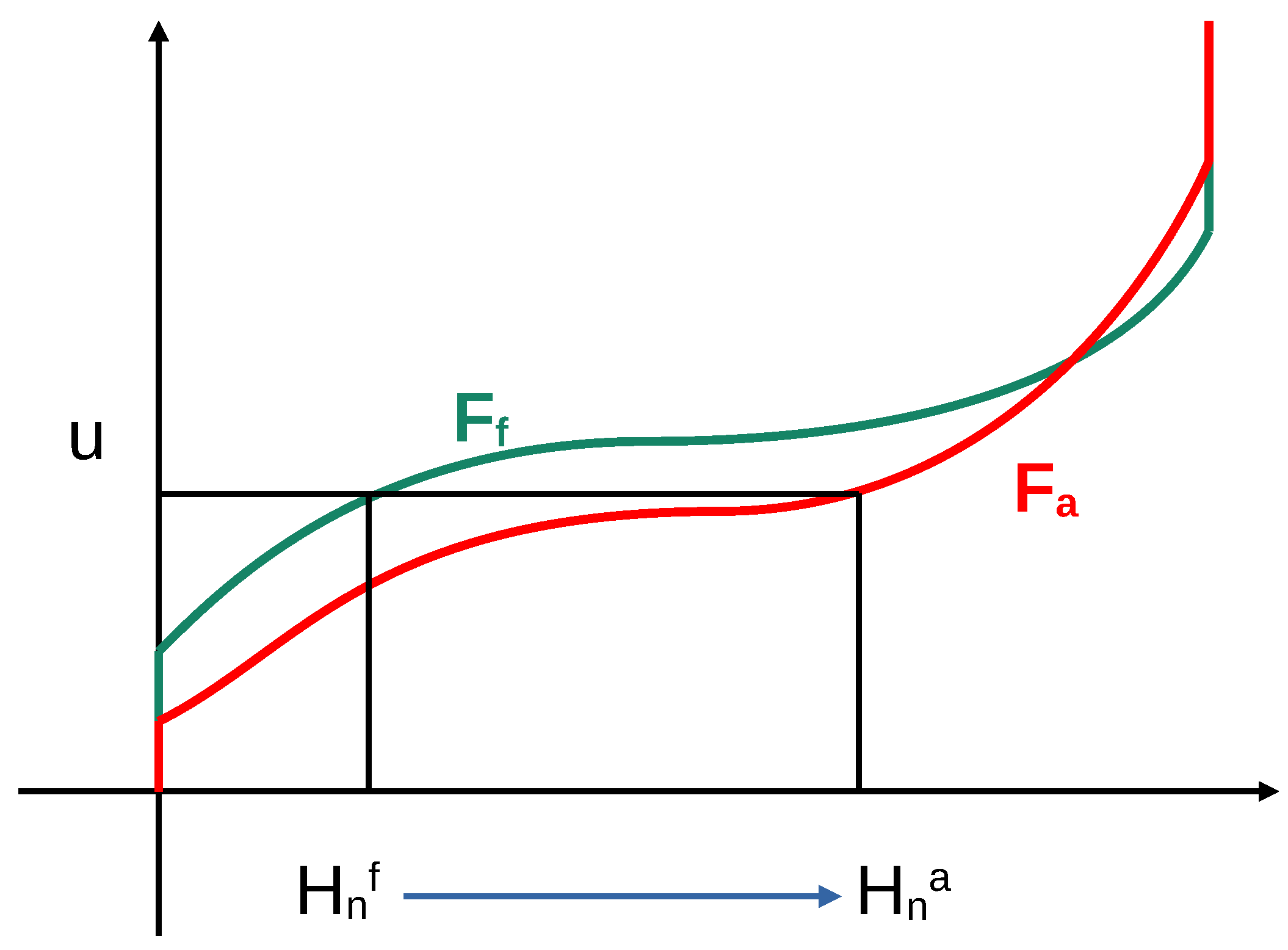
Typically, neither nor are known a priori, so they need to be estimated from the ensemble and, in the case of , from the observation value. Please note that is the quantile function for the posterior distribution and that the ensemble members retain their quantiles when moving from the forecast to the analysis. Ensemble filters that operate in this way have, therefore, recently been called ‘Quantile-Conserving Ensemble Filters’ (QCEFs [5]). The action of a QCEF on a single ensemble member is illustrated in Figure 1. Figure 1 illustrates a QCEF where the prior and posterior CDFs have jump discontinuities; the appropriate definitions of these functions and their inverses in such a case are discussed in Appendix A.
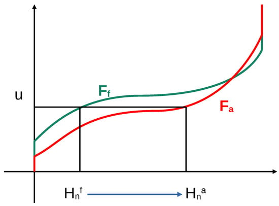
Figure 1.
An illustration of a QCEF. The prior ensemble member is mapped by the prior CDF to the value . This value is then mapped to the analysis ensemble member by the analysis quantile function . The CDFs illustrated here correspond to the case of mixed distributions on a bounded domain as discussed in Section 2.
This paper develops a new method for estimating the QCEF transform. The method uses kernel-density estimation to approximate the prior probability density function (PDF). Extra care is taken with the kernel-density estimation to handle random variables with bounded ranges, as well as to handle situations with a nonzero total probability on one or both boundaries. This estimate of the prior PDF is then integrated approximately using quadrature to produce an approximation of the prior CDF . Bayes Theorem states that, up to a normalizing constant, the posterior PDF equals the prior PDF multiplied by the likelihood function. The new method, therefore, again uses quadrature to approximate the posterior CDF ; in addition to the approximation of the prior PDF, this only requires the ability to evaluate the likelihood function. Finally, a root-finding method is applied to the equation
to solve for the analysis ensemble members .
The details of the new, nonparametric QCEF method are described in Section 2. Section 3 compares the new method to the Bounded Normal Rank Histogram Filter (BNRHF; [6,7,8]) and to an EnKF in synthetic non-Gaussian DA problems where the posterior distribution is exactly known. Section 4 then compares these methods in the context of assimilating observations of sea-ice concentration (SIC) into a single-column sea-ice model (Icepack). Conclusions are offered in Section 5.
2. Mixed Delta-Kernel Distributions
This section describes the methods used to estimate the parameters in a mixed distribution of the form
where denotes the Dirac delta distribution. Here, the random variable H is assumed to take values in the range . The constants are the total probabilities at the lower bound , in the interior , and at the upper bound . As probabilities, they are non-negative and sum to one. If then , and if then . The subscript l, m, and u stand for lower, middle, and upper, respectively, and the subscript int on stands for interior. We assume that is a probability density function in its own right, in particular that it integrates into one.
Bounded variables appear in many applications. For example, rainfall is never negative, and concentration mixing ratios are between zero and one. Bounded variables also appear in the context of parameter estimation; for example, microphysical parameters in numerical weather prediction models or albedo parameters in snow and ice models are bounded. Mixed distributions are also relevant to many applications; for example, one might make a forecast with a nonzero probability of having no rain while the remaining probability is distributed across a continuous range of possible rainfall rates. These distributions are also relevant to sea-ice data assimilation, as seen in Section 4.
We assume that the likelihood function is available up to a positive multiplicative constant, i.e.,
where denotes the probability density of observing value given that , and the proportionality constant is positive and independent of h.
In the present context, Bayes’ theorem takes the following form
where the proportionality constant is independent of h and serves only to guarantee that the total integrated probability is one. When the prior is a mixed distribution of the form Equation (5), Bayes theorem implies that the posterior distribution will also be a mixed distribution, with posterior density
The posterior class weights are given by
where denotes expectation with respect to , i.e.,
The posterior probability density in the interior is
These expressions follow from Bayes’ theorem Equation (7) where the proportionality constant, which is the denominator in Equations (9)–(11), is set to ensure unit total probability.
The remaining subsections of this section describe methods that use an ensemble , to estimate the prior and posterior class weights and interior PDF, to approximate the application of the prior cumulative distribution function (CDF) to the ensemble, and finally to approximate the application of the posterior quantile function to produce an analysis ensemble , .
2.1. Class Weights
The prior class weights are easy to estimate from the ensemble. Suppose that there are ensemble members on the left boundary (), in the middle, and on the upper boundary. Then, the prior class weights are estimated as
The only subtlety in the estimation of the posterior class weights lies in the approximation of the expected value of the likelihood function over the interior distribution. We approximate this using a simple Monte-Carlo approximation. Suppose that are in the interior; then
2.2. Interior Probability Density Using Kernel-Density Estimation
Kernel-density estimation (KDE) is a classic way of using an ensemble of realizations of a random variable to approximate the probability density function of the random variable [9]. Suppose that K is a function with non-negative output that integrates to unity and that , are independent realizations of a random variable H with PDF . Then
where are called the bandwidths and K is the kernel. Kernel-density estimation theory addresses the choice of kernel function K and bandwidths that make the approximation accurate.
We here choose to use the Epanechnikov kernel
where is the so-called Rectified Linear Unit that returns zero for negative arguments and returns the argument for non-negative arguments. We chose this kernel primarily because it has compact support and is computationally inexpensive to evaluate, though it has some other optimality properties in the context of kernel-density estimation [10].
We set the bandwidths using the adaptive method described in ([9], §5.3). This method proceeds as follows. First, we use the standard rule of thumb to set a non-adaptive bandwidth parameter
where is the standard deviation of the interior ensemble ([9], §3.4). The value 2 in this equation is specific to the Epanechnikov kernel; other kernels have different constants (cf. [4]).
Next, a ‘pilot’ estimate of the density is obtained using the nearest-neighbor method ([9], §2.5)
where is the distance from h to the kth nearest neighbor in the ensemble. We set where rounds down to the nearest integer.
This pilot estimate of the density is then used to construct local bandwidth factors
where g is the geometric mean of . These local bandwidth factors are finally used to modulate the non-adaptive bandwidth , producing adaptive bandwidths
2.3. Boundary Corrections on the Interior Probability Density
The foregoing kernel-density estimate of the probability density function is a consistent approximation even when the data come from a bounded distribution, but the order of accuracy is significantly reduced near boundaries. There are many approaches to updating the kernel-density approximation for bounded distributions. Two directions not pursued here include reflecting the data around the boundaries and transforming the data from a bounded to an unbounded distribution before performing kernel-density estimation in the unbounded domain.
The approach taken here is to locally modify the kernel near the boundary [11,12]. We define the following two functions
(The argument t here is simply a dummy variable; it does not denote time). The form of these functions depends on the choice of kernel function as described in ([12], §1); the expressions given above correspond to the Epanechnikov kernel. These functions are used to modify the jth kernel in the approximation Equation (16) near the boundary. Specifically, if the jth term is evaluated at a point h that is within a distance of the lower boundary, then the kernel is multiplied by
If the jth term is evaluated at a point h that is within a distance of the upper boundary, then the kernel is multiplied by
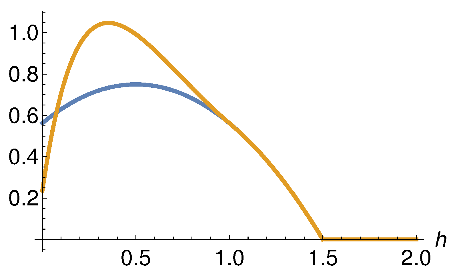
The effect of this correction on a single kernel near a lower boundary is illustrated in Figure 2 for a kernel centered at near a lower boundary at .
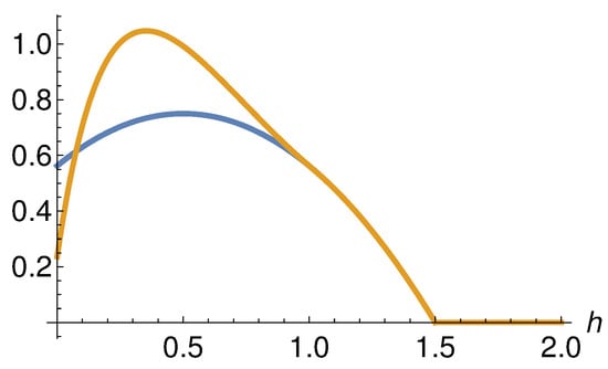
Figure 2.
Illustration of the effect of boundary correction on a kernel. The blue line shows a single kernel with and . The orange line shows the boundary-corrected kernel for a lower boundary at . For h ≥ 1 the two curves overlap.
This correction returns the accuracy of the approximation near the boundary to the same order of accuracy enjoyed by the approximation away from boundaries. In the absence of boundaries, the approximation Equation (16) integrates to unity, as required for a probability density function. The correction breaks this property so that the corrected approximation no longer integrates into unity. It must, therefore, be scaled by an appropriate factor equal to the integral of the corrected approximation over the support of the PDF. This scaling factor (inter alia) is approximated using quadrature, as described in the next subsection.
2.4. Cumulative Distribution Functions Using Quadrature and Sampling
Applying the QCEF transform requires evaluating the approximations to the prior and posterior cumulative distribution functions (CDFs) described in the previous sections. For values in the interior, i.e., not on the boundaries, this is achieved using quadrature. Before describing the quadrature, we discuss the application of the prior CDF to values on the boundary.
2.4.1. Boundary Sampling
The formal definition of as the CDF of the prior given by Equation (5) implies that
But with this formal definition, the QCEF transform Equation (1) would not produce an analysis ensemble distributed according to the true posterior distribution. As detailed in Appendix A, in order for Equation (1) to work correctly for any pair of prior and posterior distributions of the form Equations (5) and (8), should map values on the lower boundary to a uniform distribution on , and it should map values on the upper boundary to a uniform distribution on .
We achieve this as follows. First draw a single random number u from a uniform distribution on , then set
Suppose that we have prior ensemble members on the lower boundary , . Then we set
Similarly, suppose that we have prior ensemble members on the upper boundary , . Then we set
Strictly speaking, is an abuse of notation because the map defined above is multivalued, is a function of an entire ensemble rather than a single argument and is not deterministic. Ultimately, what matters is that we have a map from the forecast ensemble to a set of values that are uniformly distributed on .
The question of how to define for boundary values was addressed in [8] in the context of the Bounded Normal Rank Histogram Filter (BNRHF). They chose to map all members on the boundary to the middle of the corresponding interval, e.g., ensemble members on the lower boundary map to the value . On the one hand, this preserves the property that identical ensemble members are all treated identically, whereas the approach taken here arbitrarily separates identical ensemble members. On the other hand, as will be seen in Section 3, this choice leads to an inability to correctly represent the posterior in certain cases.
2.4.2. Quadrature
For any , the kernel-density approximation to the interior prior CDF is
The kernel approximation to the interior PDF is piecewise-smooth, with discontinuous derivatives at the points , where is the radius of kernel that is centered at . We begin by defining breakpoints that consist of the points and the points and (if they are finite). These points are sorted, and any points outside the range are discarded. The remaining points define a set of subintervals . If then we have
In the absence of boundary corrections, these integrals can be evaluated by integrating the Epanechnikov kernel. In the presence of boundary corrections, it is possible, but tedious, to compute the integrals analytically; for the posterior interior CDF, the integrand is multiplied by the likelihood function , so none of the integrals can be computed analytically. In these cases, we approximate each of these integrals using Gauss-Legendre quadrature with five-points, which is exact for polynomials up to degree nine ([13], §5.3). The integrals pre-computed on each sub-interval using Gauss-Legendre quadrature to save computational cost so that a single evaluation of the CDF requires only computing the final integral
and adding it to the sum of the pre-computed integrals. New integrals must be pre-computed for each new forecast, so the savings are not as great as they would be if it were possible to pre-compute values once and use them for all forecasts.
2.5. Application of the Quantile Function Using Root-finding
The QCEF probability integral transform Equation (1) requires inverting the approximation to the posterior CDF. This is accomplished via root-finding methods. We define the function
If then , as desired.
To obtain a first guess for the solution, we use the pre-computed values discussed in the previous section to form a piecewise-linear approximation to between the points . The root of this piecewise-linear approximation can be found analytically and serves as the first guess supplied to the root-finding algorithm.
The root-finding method starts with the secant method ([13], §2.3), which produces a sequence of approximations to the root. This continues until either (i) the tolerance () is met, (ii) the max number of iterations (50) is reached, or (iii) two consecutive approximations bracket the root. If (iii) occurs, i.e., if two approximations of are found that produce values of f with opposite sign, then the algorithm switches to an improved bisection method from [14] called the ‘Interpolation, Truncation, and Projection (ITP) method’, which terminates either when the tolerance is met, or the max number of iterations is reached. The root-finding problems that need to be solved to update the ensemble are independent of each other and can, therefore, be carried out in parallel, but the implementation used here does not make use of parallelism.
The worst-case performance of the combined secant-ITP method is that of the bisection method, i.e., the error reduces by a factor of 2 at each iteration (linear convergence). The method will, therefore, reach the tolerance before hitting the maximum number of iterations as long as the initial error is less than . The best performance comes from the case where the method never switches from secant to ITP; in this case, the order of the method is between linear and quadratic, with exponent ([13], Theorem 2.3). Using the configuration recommended in [14], the best-case performance of the ITP method is convergence with order .
The computational bottleneck in a single iteration of the root-finding method is the evaluation of the CDF . If the integrals on the subintervals were not pre-computed as described in the previous section, then these integrals would have to be re-computed at every step of the root-finding iteration, and for every ensemble member, the pre-computation thus leads to significant savings. With the pre-computation, the most expensive part of a single evaluation of the CDF is the computation of the Gauss-Legendre approximation to the integral on a single sub-interval Equation (31), which requires evaluating five times.
3. Non-Cycling Tests
This section compares three ensemble filters on three scalar problems where the answer is known analytically. The three algorithms are
- The Ensemble Adjustment Kalman Filter (EAKF; [15]),
- The Bounded Normal Rank Histogram Filter (BNRHF; [7,8]),
- The Kernel-based QCEF (KQCEF) developed in the preceding section.
The EAKF is a deterministic ensemble Kalman filter. It assumes that the prior and likelihood are Gaussian, which implies that the posterior is also Gaussian. Under these assumptions, an affine transformation of the forecast ensemble will produce an analysis ensemble with the correct mean and variance. The EAKF estimates the parameters of this affine transformation using the forecast ensemble and the observation information and then applies the resulting transformation to the forecast ensemble members.
The BNRHF is a QCEF that updates the RHF of [6]. The prior PDF is approximated as piecewise-constant between ensemble members, with Gaussian tails outside the ensemble. The likelihood is evaluated by the ensemble members and linearly interpolated between ensemble members. The posterior PDF is, therefore, piecewise-linear between the ensemble members. The prior CDF and posterior quantile function are then combined per Equation (1) to update the ensemble members.
The ensemble size varies through , and at each ensemble size, the test is repeated 100 times. In all three problems, the likelihood is normal
The tests and their results are presented in the following subsections.
In each test, we generate an ensemble drawn from the prior, apply the three filters above to the same prior ensemble, and use the Kolmogorov–Smirnov (KS; [16]) test on the null hypothesis that the analysis ensemble is drawn from the known posterior distribution. A drawback of this (or any) test of the null hypothesis that the analysis ensemble is drawn from the true posterior distribution is that the null hypothesis can be rejected even when the analysis ensemble is drawn from a distribution that is close to the true posterior distribution. (Naturally, if the analysis distribution is close to the true posterior distribution, then it takes a large ensemble to confidently reject the null hypothesis). The KS test could, for example, reject the null hypothesis in a situation where the analysis ensemble mean has a very small error, but the shape of the analysis ensemble clearly does not reflect the true posterior distribution.
An alternative would be to directly estimate a distance (or divergence) between the analysis and true posterior distributions, e.g., using the Kullback–Leibler (KL) divergence. A strength of the KL divergence as compared to the KS test is that the KL divergence provides a number representing the error in the analysis distribution (whereas the KS test accepts or rejects the null hypothesis). A weakness of the KL divergence is that it can be hard to interpret, whereas the KS test has a very clear meaning. Like the KS test, sample-based estimates of the KL divergence are sensitive to ensemble size [17,18].
3.1. Normal Prior
In this problem, the prior is Gaussian, with mean zero and unit standard deviation. The posterior is, therefore, also Gaussian, with known mean and variance. In addition to varying the ensemble size, we also vary the value y of the observation and the observation error standard deviation . If y is far from 0, then the observation is in the tail of the prior distribution. If , then the observation error is small compared to the prior.
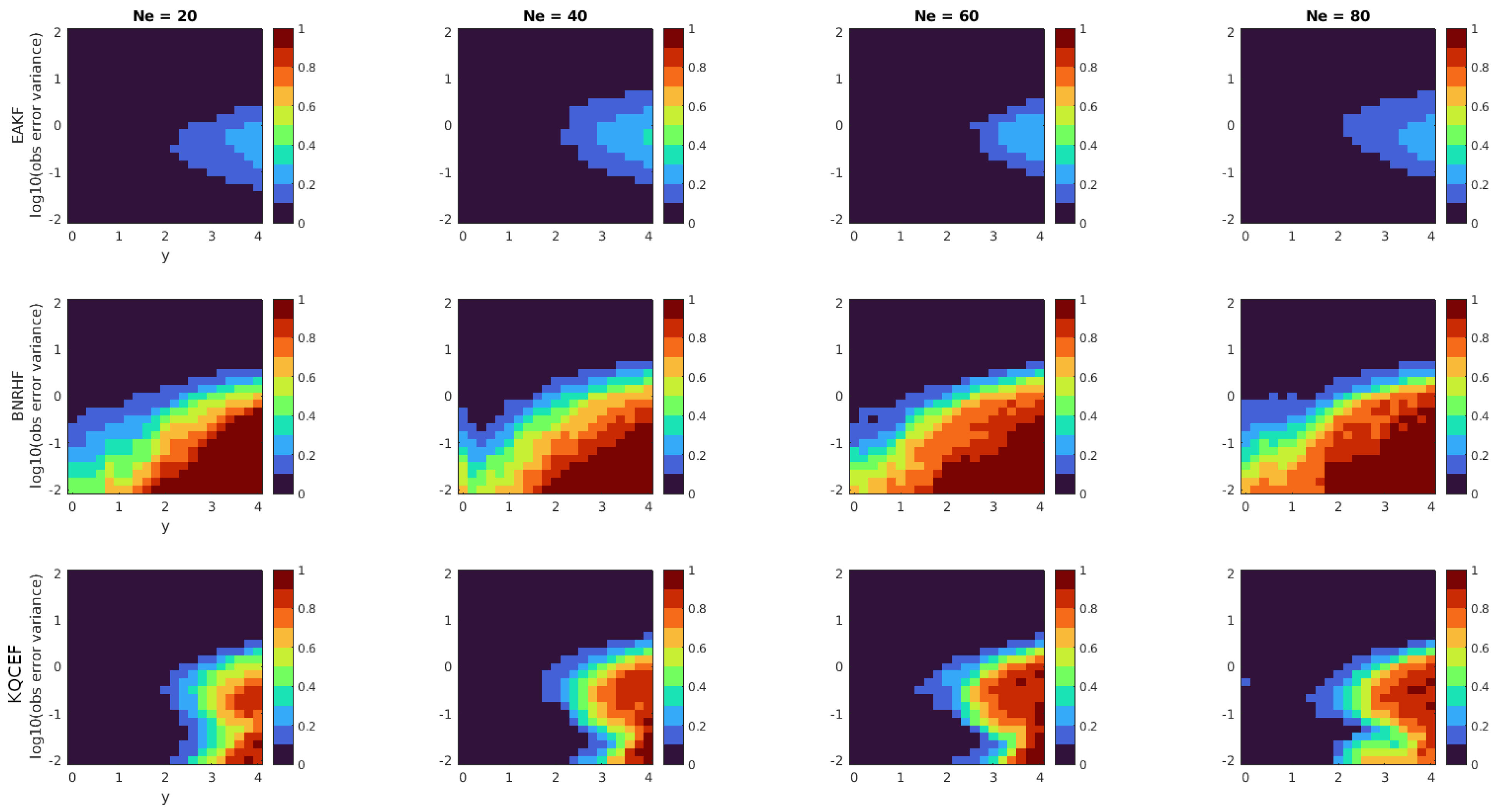
Each panel in Figure 3 shows the fraction of times that the KS test rejected the null hypothesis at the 5% significance level. The horizontal axis shows the value of y, while the vertical axis shows the logarithm of the observation error variance. Low values indicate that the analysis ensemble produced by the ensemble filter was frequently consistent with the true posterior distribution. The top row shows the EAKF results, the middle row shows the BNRHF results, and the bottom row shows the KQCEF results. The columns show the results for , and 80, from left to right.

Figure 3.
Each panel shows the fraction of 100 experiments where the null hypothesis that the analysis ensemble was drawn from the known true posterior distribution was rejected by the Kolmogorov–Smirnov test at the 5% significance level. The prior is a standard normal. The likelihood is normal with mean y that varies along the horizontal axis and variance that varies along the vertical axis. The EAKF, BNRHF, and KQCEF results are in the upper, middle, and lower rows. The ensemble size varies across the columns from 20 to 80.
It is seldom the case in practice that the forecast comes from a known family of parametric distributions and that the likelihood is conjugate to the prior. But in those cases, or in cases where the forecast distribution is well-approximated by a parametric distribution that is conjugate to the likelihood, one expects that a filter based on conjugate parametric distributions (cf. the methods discussed in [5,19]) will outperform nonparametric approaches like the BNRHF and KQCEF. That is indeed the case here: the prior and likelihood are both normal, which precisely matches the assumptions of the EAKF, and we see that the EAKF performs best of the three algorithms in this test. The only source of errors in the EAKF is sampling errors in estimating the prior mean and variance. These sampling errors decrease as the ensemble size increases, but so does the sensitivity of the KS test; combined, these effects lead to minimal changes in the accuracy across ensemble sizes. The EAKF performs well overall but slightly less well when the observation is in the tail of the prior and when the observation error variance is comparable to the prior variance.
All the methods perform well when the observation error variance is large compared to the prior variance, regardless of the value of y. This is reassuring because the analysis ensemble should only be minimally changed compared to the forecast ensemble when the observation error variance is large.
When the observation value y is in the tail of the prior, neither BNRHF nor KQCEF performs well. Again, this is not surprising because the representation of the tails of the prior and posterior in the BNRHF and KQCEF relies on ensemble members in the tails, and there are, by definition, not many ensemble members in the tails.
The only benefit of the KQCEF over the BNRHF in this problem comes when the observation error variance is small compared to the prior variance and the observation value is not too far into the tails of the prior. In such cases, the KQCEF significantly outperforms the BNRHF. This is because the BNRHF approximates the likelihood by evaluating it at ensemble members and linearly interpolating between ensemble members; when the observation error is small compared to the prior spread, the gaps between ensemble members can be so large that the piecewise-linear approximation of the likelihood is inaccurate. See Section 5.1 for further discussion of this issue.
3.2. Bi-Normal Prior
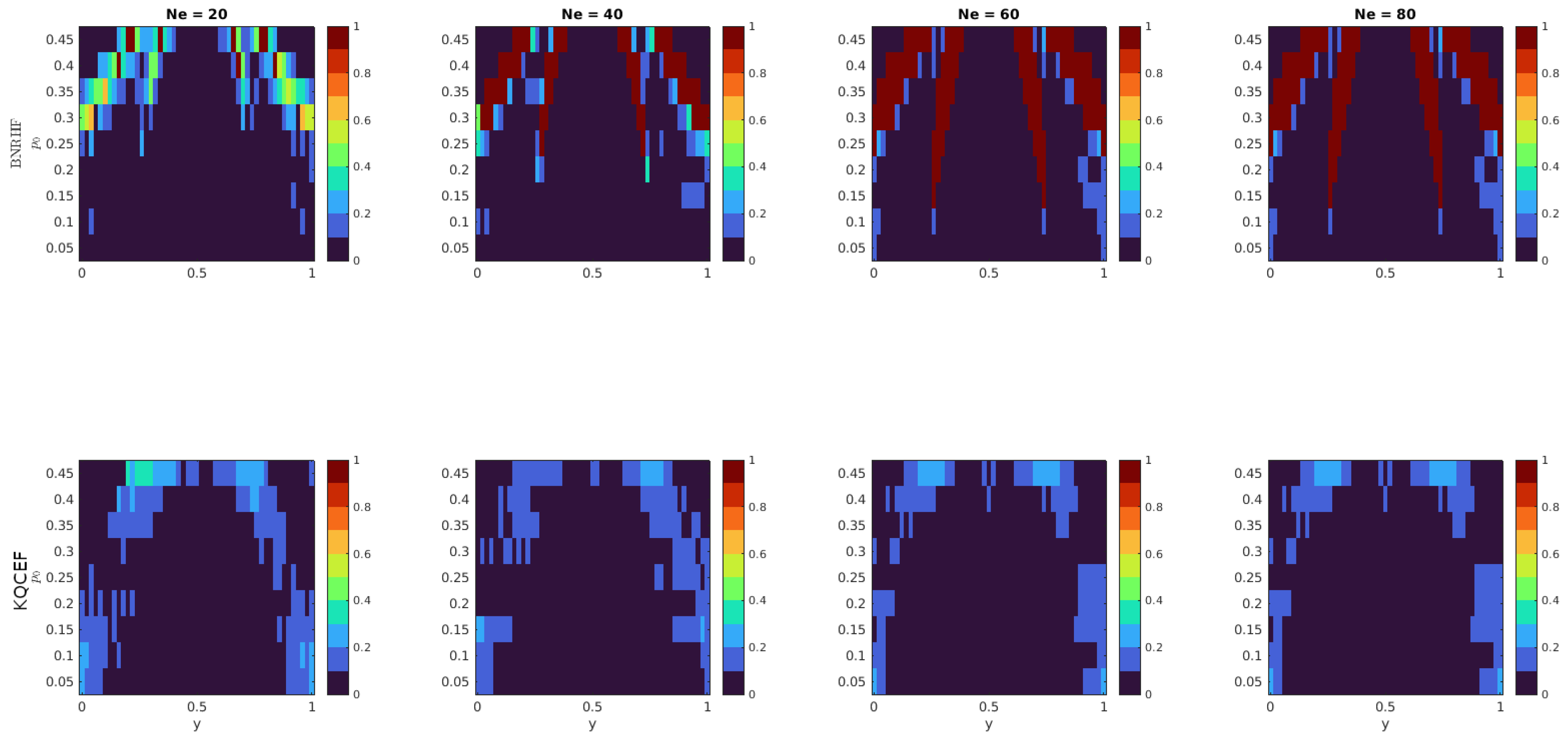
In this problem, the prior is a Gaussian mixture with two equally weighted components, each of which has a unit standard deviation. One component is centered at while the other is centered at 2. The posterior is, therefore, also a Gaussian mixture, where the class weights, means, and variances are known functions of the observation value and observation error variance. As in the previous problem, in addition to varying the ensemble size, we also vary the value y of the observation and the observation error standard deviation .
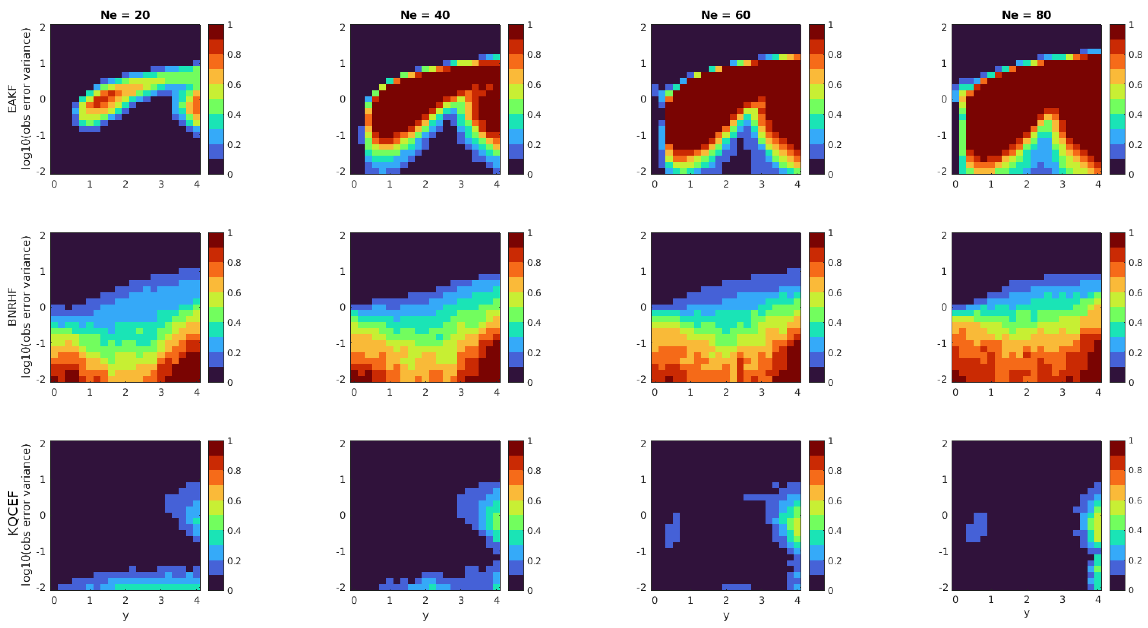
Each panel in Figure 4 shows the fraction of times that the KS test rejected the null hypothesis at the 5% significance level. The arrangement of the panels is the same as Figure 3. The KQCEF performs the best of the three algorithms in this test. As in the normal problem, the errors are largest (but still not too large) when the observation is in the tail of the prior, and the observation error variance is close to one. The errors are smaller here than in the normal problem because an observation value of is only two standard deviations from one of the Gaussian modes of the prior, whereas, in the normal problem, an observation value of is four standard deviations from the mean of the prior. There are also slightly elevated error levels when the observation error variance is small and the ensemble size is small. These appear presumably because the ensemble members are being split between the two modes of the prior, and each mode is poorly resolved.
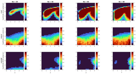
Figure 4.
Each panel shows the fraction of 100 experiments where the null hypothesis that the analysis ensemble was drawn from the known true posterior distribution was rejected by the Kolmogorov–Smirnov test at the 5% significance level. The prior is an equal mixture of two normals, each with unit variance, with means at −2 and 2. The likelihood is normal with mean y that varies along the horizontal axis and variance that varies along the vertical axis. The EAKF, BNRHF, and KQCEF results are in the upper, middle, and lower rows. The ensemble size varies across the columns from 20 to 80.
The BNRHF performs well on this problem only when the observation error variance is large, in which case all the methods perform well. When the observation error variance is small, the BNRHF performs worse than the EAKF. In this case, the problem exhibits what some authors have called ‘medium nonlinearity’ [20,21]: The prior is very non-Gaussian, but the posterior is approximately Gaussian. In such cases, the EAKF effectively ignores the prior and moves all the ensemble members closer to the observed value y. The BNRHF uses an approximation of the likelihood function and posterior PDF that is piecewise-linear between the ensemble members. If the likelihood is so tight that the structure of its peak falls between ensemble members, then the BNRHF cannot correctly represent the posterior PDF, which leads to errors. See Section 5.1 for further discussion of this issue.
When the observation error variance is close to the prior variance, the EAKF performs very poorly. But more importantly, the EAKF errors increase as the ensemble size increases. This is because the EAKF uses an affine transformation to update the ensemble members, and this affine transformation preserves the equally weighted bimodal structure of the prior. As the ensemble size increases, the KS test becomes more sensitive and can tell the difference between the unequally weighted bimodal structure of the true posterior and the equally weighted bimodal structure produced by the EAKF.
3.3. Mixed Prior
In this problem, the prior is a mixed distribution on consisting of delta distributions at and each with probability and a truncated normal in the interior with mean and variance (of the un-truncated normal) . The observation error variance is fixed at , and the observation value y is varied between zero and one. The posterior is, therefore, also a mixed distribution with delta distributions on the boundaries and a truncated normal in the interior, and all the class weights and truncated-normal parameters can be computed in terms of the parameters of the prior and likelihood.
The EAKF can produce analysis ensemble members outside the range . It is possible to update the EAKF so that it respects the bounds, e.g., by truncating values outside the boundary back to the boundary. The ad-hoc updates amount to an unfair comparison with the more sophisticated BNRHF and KQCEF, though, so we refrain from testing the EAKF on this problem and compare only the BNRHF and KQCEF.
The value of controls the initial number of ensemble members on the boundaries. For , there are no forecast ensemble members on the boundaries, and neither BNRHF nor KQCEF will move ensemble members onto the boundary when there are none initially, regardless of the value of y. The test with tests the ability of BNRHF and KQCEF to handle cases with bounded variables.
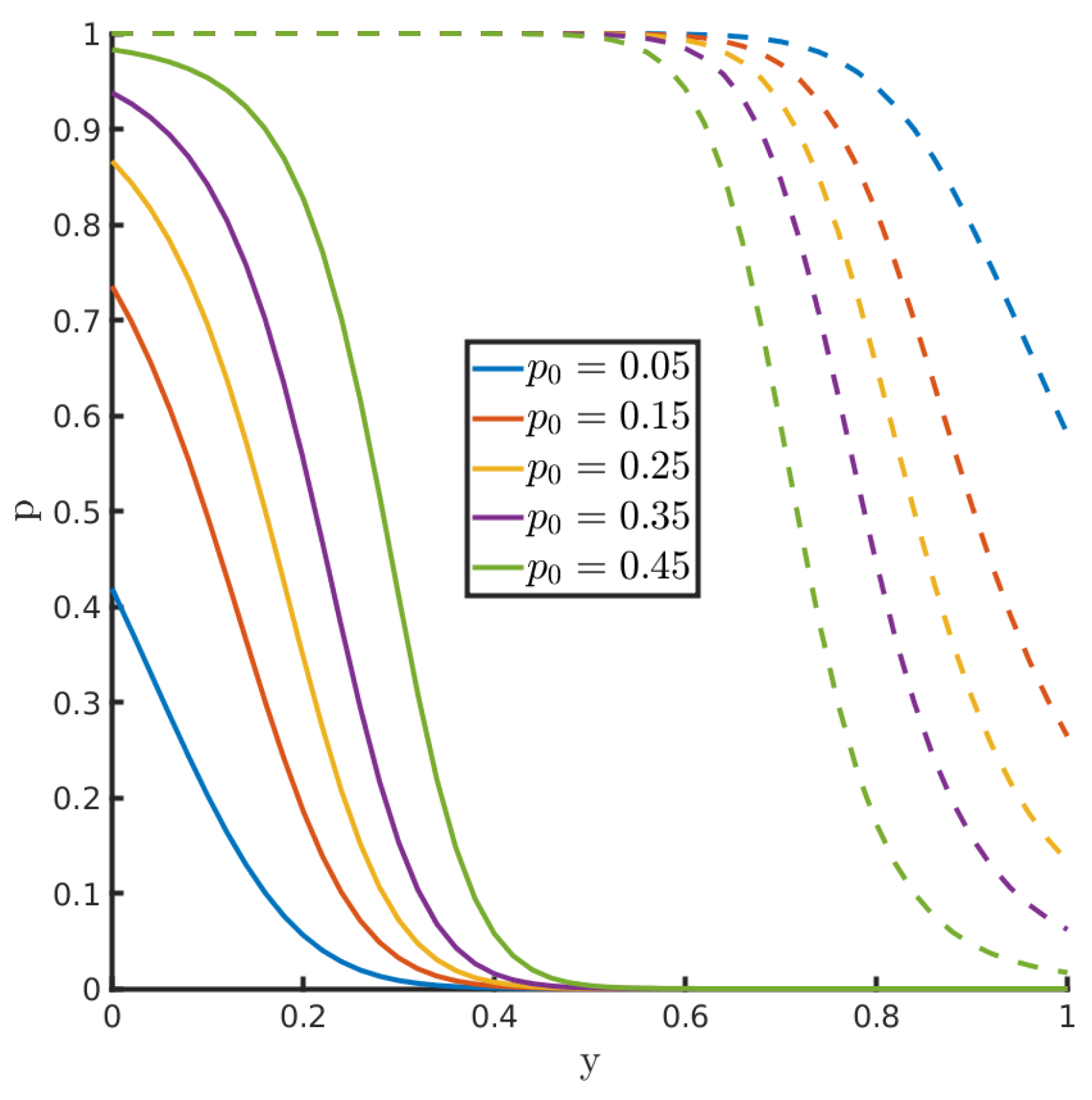
As increases from zero, the number of forecast ensemble members on the boundaries increases. For a fixed positive value of , the value of y controls how many ensemble members move from or onto each boundary. This is illustrated in Figure 5. The value y varies along the horizontal axis. At a fixed value of y, the posterior probability for each class (lower boundary, interior, upper boundary) is indicated by the lines, which divide the vertical axis between the three classes. Each color corresponds to a different value of ; the distance below the solid lines indicates the posterior probability on the left boundary; the distance between the solid and dashed lines indicates the posterior probability in the interior; and the distance above the dashed lines indicates the posterior probability on the right boundary. For example, when we see that the posterior probability is almost entirely in the interior for all values of , meaning that all ensemble members on the left and right boundaries should all move to the interior when .
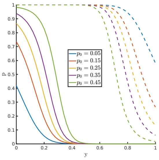
Figure 5.
Division of the total posterior probability between the left boundary, interior, and right boundary as a function of the observation value y for the test with mixed and bounded prior. Each color corresponds to the prior probability on each boundary. The solid line indicates the posterior probability on the left boundary; the distance between the solid and dashed lines indicates the posterior probability in the interior; and the distance from the dashed line to 1 indicates the posterior probability on the right boundary.
As another example, suppose that , meaning that when , the prior ensemble has one member on each boundary. If , then the posterior probability on the left boundary is approximately , so we expect to have approximately 8 posterior ensemble members on the left boundary. In this case, the posterior probability on the upper boundary is near zero, so the remaining 12 posterior ensemble members should be in the interior.
In this problem, we test two aspects of the posterior separately. The analysis ensemble produced by each filter allocates a certain number of ensemble members to each class (left boundary, interior, right boundary). This distribution of ensemble members between classes should be statistically indistinguishable from a draw from a multinomial distribution, so we begin by testing the null hypothesis that the analysis ensemble, condensed to just numbers-per-class, is a draw from the multinomial distribution whose parameters correspond to the true posterior.
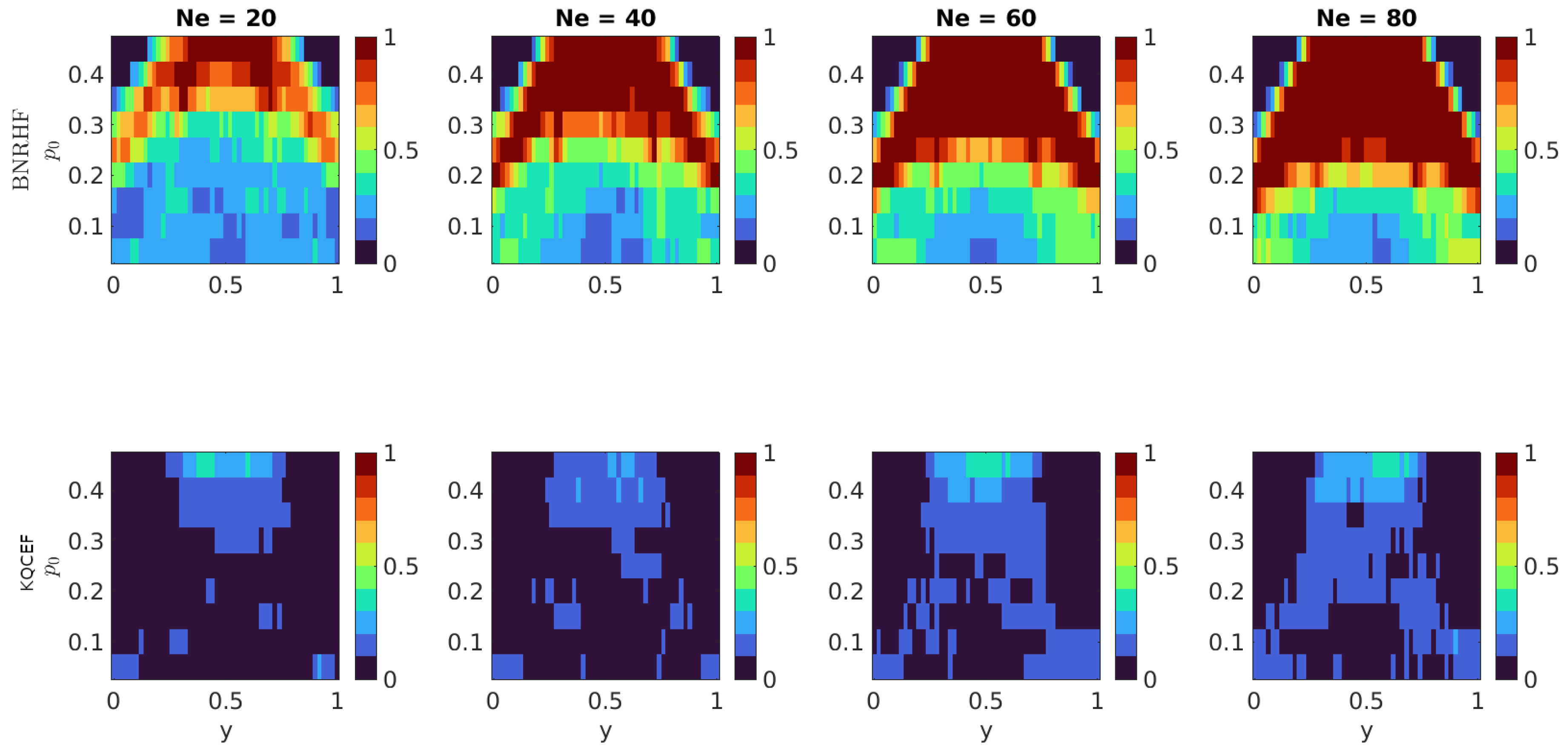
Figure 6 shows the fraction of times that the multinomial test rejected the null hypothesis at the 5% significance level. The horizontal axis shows the value of y, while the vertical axis shows the value of . The KQCEF performs better than the BNRHF in this test. At each ensemble size, there are combinations of and y where BNRHF fails the multinomial test 100% of the time. The reason for these failures is that the BNRHF moves ensemble members off the boundary all at once or not at all. For some combinations of and y, the true posterior requires some of the ensemble members on the boundary to move off the boundary and into the interior. For other combinations of and y, the true posterior requires some of the ensemble members on the boundary to move into the interior and some onto the other boundary. For these combinations of and y, the analysis ensemble produced by the BNRHF either moves all or none of the members from the boundary, which is different enough from the true posterior that it fails the test, especially when the prior ensemble members on the boundary should be split in half. As the ensemble size grows, the difference between half and all (or between half and none) grows, making the error more egregious. The KQCEF has some difficulty in similar regions of parameter space but is still very accurate.
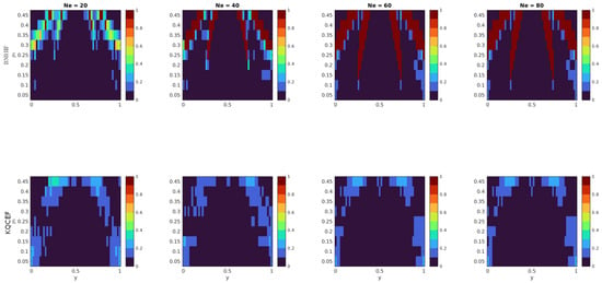
Figure 6.
Each panel shows the fraction of 100 experiments where the null hypothesis was rejected at the 5% significance level. The null hypothesis is that the number of posterior ensemble members on the left and right boundaries and in the interior is consistent with a trinomial distribution whose parameters are the known true probabilities on the boundaries and in the interior. The prior is a mixed distribution with probability on both the left and right boundaries and a truncated normal prior in the interior. The value of varies along the vertical axis. The likelihood is normal with mean y that varies along the horizontal axis and variance . The BNRHF and KQCEF results are in the upper and lower rows, respectively. The ensemble size varies across the columns from 20 to 80.
We also use the KS test to determine the accuracy of the distribution of the interior ensemble members. The true posterior distribution in the interior is a truncated normal with known parameters, and we use the KS test to test the null hypothesis that the analysis ensemble members in the interior (regardless of how many there are in the interior) are drawn from the true posterior distribution in the interior. The results are shown in Figure 7. The problem is particularly difficult when is large because, in this case, there are many prior ensemble members on the boundaries and few in the interior. BNRHF and KQCEF both use the interior ensemble members to estimate the interior distribution, but when there are few interior ensemble members, the approximation of the interior distribution is inaccurate. This is reflected in the results, particularly near because when y is near the middle of the interval, the posterior probability is almost entirely in the interior (cf. Figure 5). On the other hand, for values of and y where the posterior has very few ensemble members in the interior (e.g., for large and y near one of the boundaries), both filters perform well according to this test. The reason for this is that the sensitivity of the KS test depends on the sample size; in situations where there are very few analysis ensemble members in the interior it is hard to tell whether they are distributed correctly or not.
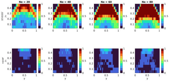
Figure 7.
Each panel shows the fraction of 100 experiments where the null hypothesis that the analysis ensemble in the interior was drawn from the known true posterior distribution in the interior was rejected by the Kolmogorov–Smirnov test at the 5% significance level. The prior is a mixed distribution with probability on both the left and right boundaries and a truncated normal prior in the interior. The value of varies along the vertical axis. The likelihood is normal with mean y that varies along the horizontal axis and variance . The BNRHF and KQCEF results are in the upper and lower rows, respectively. The ensemble size varies across the columns from 20 to 80.
Overall, the KQCEF performs significantly better than the BNRHF in this test. This can again be traced back, at least in part, to the fact that the BNRHF moves all the boundary ensemble members together or not at all. When is large there are many prior ensemble members on the boundaries. If y is near , then BNRHF correctly moves the boundary members into the interior, but it moves all the members from the left boundary to one location in the interior and all the members from the right boundary to another location in the interior. The prior distribution had delta distributions on the boundaries, and the analysis produced by BNRHF incorrectly moves these delta distributions into the interior. The KS test notices these jumps in the interior and flags the BNRHF analysis distribution as being significantly different from the true posterior. That said, the KQCEF also outperforms the BNRHF even when , i.e., there are no ensemble members on the boundary, but in this case, the BNRHF performs better than it does when . The EAKF was not tested on this problem, but it also moves all members from the boundary to the same location in the analysis and, therefore, suffers the same problem (in addition to the problem of not respecting the bounds).
4. Application to Sea-Ice Concentration
Assimilation of satellite observations of sea ice provides an excellent example of a data-assimilation problem with bounded, non-Gaussian distributions. We follow [22] in using the single-column version of the CICE sea-ice model, called Icepack [23], to explore how advances in nonlinear, non-Gaussian data-assimilation algorithms might lead to improvements in sea-ice data-assimilation.
The model represents sea ice in a single grid cell. Within this grid cell, there are five categories of ice thickness, not counting open water (zero thickness). For each category, the model tracks a range of variables, notably including the fraction of the grid cell area that is covered by ice within that category, as well as the total volume of ice in that category. The mean thickness within a category is given by the volume divided by the area fraction, and the mean thickness lies between the thickness bounds that define the category. Each ice category is covered by some amount of snow, and the model tracks the total volume of snow covering each category; the snow thickness covering an ice category is equal to the snow volume covering that category divided by the area fraction of the category. The variable of interest here is the total sea-ice concentration (SIC), equal to the sum of the area fractions of the five ice categories; it is also equal to one minus the fractional area of the grid cell that has no ice cover (i.e., open water). Although we investigate the method in the context of the CICE model, the approach developed here could be applied to any model that has SIC as a state variable, e.g., the SIS [24], neXtSIM [25], and SI3 [26] models.
4.1. SIC Likelihood
There are several satellites whose sensors return data relevant to SIC, and observations of SIC have been assimilated into sea-ice models for decades [27,28,29,30,31,32,33,34,35]. Assimilating data from any particular satellite requires an observing model appropriate to that satellite; we introduce such a model here. We assume that as the satellite tracks across a single grid cell (corresponding to the Icepack model), it makes measurements at points within the grid cell. At each point, it observes whether there is ice or open water; k of the points have open water. This model is relevant to, for example, the laser altimeters aboard the ICESat-2 platform [36]. ICESat-2 provides more information than just ice vs no ice; assimilation of sea-ice thickness observations is an important topic, but it is out of the scope of the present investigation.
We model the observations as a sample from a binomial distribution with parameters and , where is the open water area fraction within the grid cell, i.e., one minus the SIC. The likelihood function is therefore proportional to a beta distribution with parameters and :
The likelihood function is all that the BNRHF and KQCEF filters need to assimilate the observational data; the EAKF requires a Gaussian approximation of the likelihood. The likelihood, when viewed as a function of has a mean
and variance ([37], §25.3)
We provide these values to the EAKF as the observation value and observation error variance. Please note that in the limit , the observation error variance goes to zero. As described below, we use either or . The former produces a larger observation error variance, while the latter produces a smaller observation error variance. The Gaussian approximation of the likelihood is accurate in the configuration with .
4.2. Experimental Design
We perform data assimilation over a single year (2011) at 75.54°N, 174.45°E. This location is between the East Siberian and Chukchi Seas; unlike areas nearer the center of the Arctic icepack, this area experiences large changes in SIC over the course of the year. Each ensemble member is forced by atmospheric conditions from distinct members of the CAM6 + DART reanalysis [38]. Each ensemble member includes a slab ocean within Icepack. The initial conditions and lateral heat flux convergence forcing are the same for all ensemble members; they are derived from the ocean component output of a fully coupled historical simulation of the Community Earth System Model [39].
Even with each member being forced by a different atmosphere, the ensemble spread is small, as the dynamics are not chaotic, and variability associated with lateral processes is missing in the single-column model. To introduce greater ensemble spread, three snow parameters of the Icepack model are perturbed:
- The R_snw nondimensional snow-albedo parameter is varied between and 0
- The rsnw_mlt melting snow-grain radius parameter is varied between and m
- The ksno parameter determining the thermal conductivity of snow varies between 0.2 and 0.35 W/m/degree.
These ranges are a subset of the prior ranges for these values in [40]. The edges of these parameter ranges were manually tuned to produce a free-running ensemble with a wide range of summer sea-ice concentrations.
The left panel of Figure 8 shows the SIC for free-running (no DA) ensemble from July through October. Outside of this window, the SIC is nearly 100% for all ensemble members. The icepack begins to melt in late July, and the freeze-up occurs between late September and early October, depending on the ensemble member. The combination of perturbed snow parameters and different atmospheric forcing produces a wide range of minimum values for SIC, from less than 10% to more than 90%.
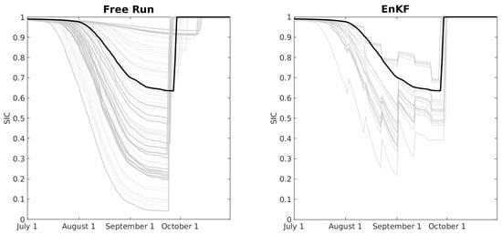
Figure 8.
Left panel: SIC as a function of time for a free-running ensemble of 79 members (grey) and a reference member (black). Right panel: SIC as a function of time for an ensemble of size 20 using the EAKF to assimilate observations of SIC every 10 days.
There are 80 ensemble members total because there are 80 distinct atmospheric forcing conditions in the CAM6 + DART reanalysis. The black line denotes the reference member that is used to produce synthetic observations in an observing system simulation experiment (OSSE). We run data-assimilating experiments with two ensemble sizes: 20 and 79; the latter is the largest ensemble possible when reserving one of the 80 total members to be the reference case. To reassure the reader that the 20 members of the smaller ensemble span the full range of behaviors as seen in the full ensemble, the members of the ensemble of size 20 are shown with slightly thicker lines in the left panel of Figure 8.
The right panel shows the results from an EnKF run with a 20-member ensemble assimilating observations every 10 days. When all the ensemble members have SIC close to 1, i.e., at the beginning and end of the plot, as well as in the time period excluded from the plot, the analysis has very little impact on the ensemble. This is because the forecast ensemble spread is very small compared to the uncertainty in the observations, so the observations are effectively ignored. Ignoring the observations in this context is not necessarily a bad thing because the ensemble forecast is very close to the reference value anyway.
Satellites providing altimeter-based ice observations have a range of repeat periods; for example, ICESat-2 has a 91-day repeat period, and CryoSat-2 has a 369-day repeat period but provides uniform coverage of the Arctic approximately every 30 days. With a 30-day observation interval, we would have only 2 or 3 assimilation cycles within the window of time where SIC is dynamically changing, and it would be hard, on the basis of only 2 or 3 assimilation cycles, to discover statistically robust differences between the performance of different filters. Microwave-scanning radiometers like AMSR-E have much more frequent repeats, providing near-uniform coverage of the Arctic daily, but pragmatic considerations lead to weekly assimilation cycles in many operational settings (e.g., [41]). We use a 10-day window as a compromise.
With a 10-day window, there are approximately 7 analysis cycles in the period between the beginning of the summer melt and the fall freeze-up. Since there are still too few cycles to obtain robust statistics, for each experimental configuration (described below), we run 10 experiments, and each experiment shifts the day of the first assimilation cycle by one day. In this way, we end up with data from assimilation cycles every day of the year while maintaining a 10-day window between cycles.
Experimental Configurations
We use two sets of ensemble sizes: and . The 79-member ensemble results from the fact that we only have 80 different atmospheric forcings from the CAM6 + DART reanalysis and one of them serves as the reference. We assimilate either or observations at each cycle. All experiments with use a single set of observations, and all experiments with use a single set of observations.
We use a two-step assimilation cycle. In the first step, we use EAKF, BRNHF, or KQCEF to assimilate the open water fraction of . Whenever EAKF produces an outside of , we map the offending value back to the nearest edge of the allowable interval.
In the second step, we update the area fraction and ice volume for each ice category in the same, simple way: If is the open water fraction in the forecast and is the open water fraction after assimilation, then the area fraction for each category is multiplied by . I.e., if the open water fraction increases, then the area fractions for all the ice thickness categories decrease by a fixed factor, and vice versa. The ice thickness and snow thickness for each category are not changed by the analysis. More sophisticated methods for updating the ice and snow thicknesses are important research topics (cf. [22]); the method used here is designed to put all the models on an even footing and to focus attention on the first step—the update in observation space. The method used here is analogous to the method used in a recent version of the TOPAZ4 ocean-ice data-assimilation system [42,43].
4.3. Results
With three filters, two observing systems ( or 100), two ensemble sizes ( and 79), and 10 experiments for each configuration, we eventually run 120 years of cycling data assimilation. To assess the performance of the filters, we compute the continuous ranked probability score (CRPS [44,45]) using the forecast and analysis ensembles at each assimilation cycle. The CRPS measures the accuracy of the probabilistic estimate provided by the ensemble; lower values are better. Specifically, the CRPS is the norm of the difference between the empirical CDF associated with the ensemble and a Heaviside step function centered on the reference value. The best possible CRPS is, therefore, zero, which can only be attained if all the ensemble members are equal to the reference value. It bears noting that the true Bayesian posterior would not have a CRPS of zero except in the very rare situation where the true posterior is a Dirac delta centered on the reference value. CRPS values have the same units as the quantity of interest, in this case, SIC. Thus, a CRPS of 0.001 corresponds to a 0.1% SIC error, which is relatively small.
For a single experimental configuration (filter, , ), we compute 58 CRPS values from 1 August through 28 September. (Outside this window, there is little difference in performance between the filters.) These 58 values come from different experiments: One experiment has assimilation cycles on 1 August, 11 August, etc., while another experiment has assimilation cycles on 2 August, 12 August, etc.
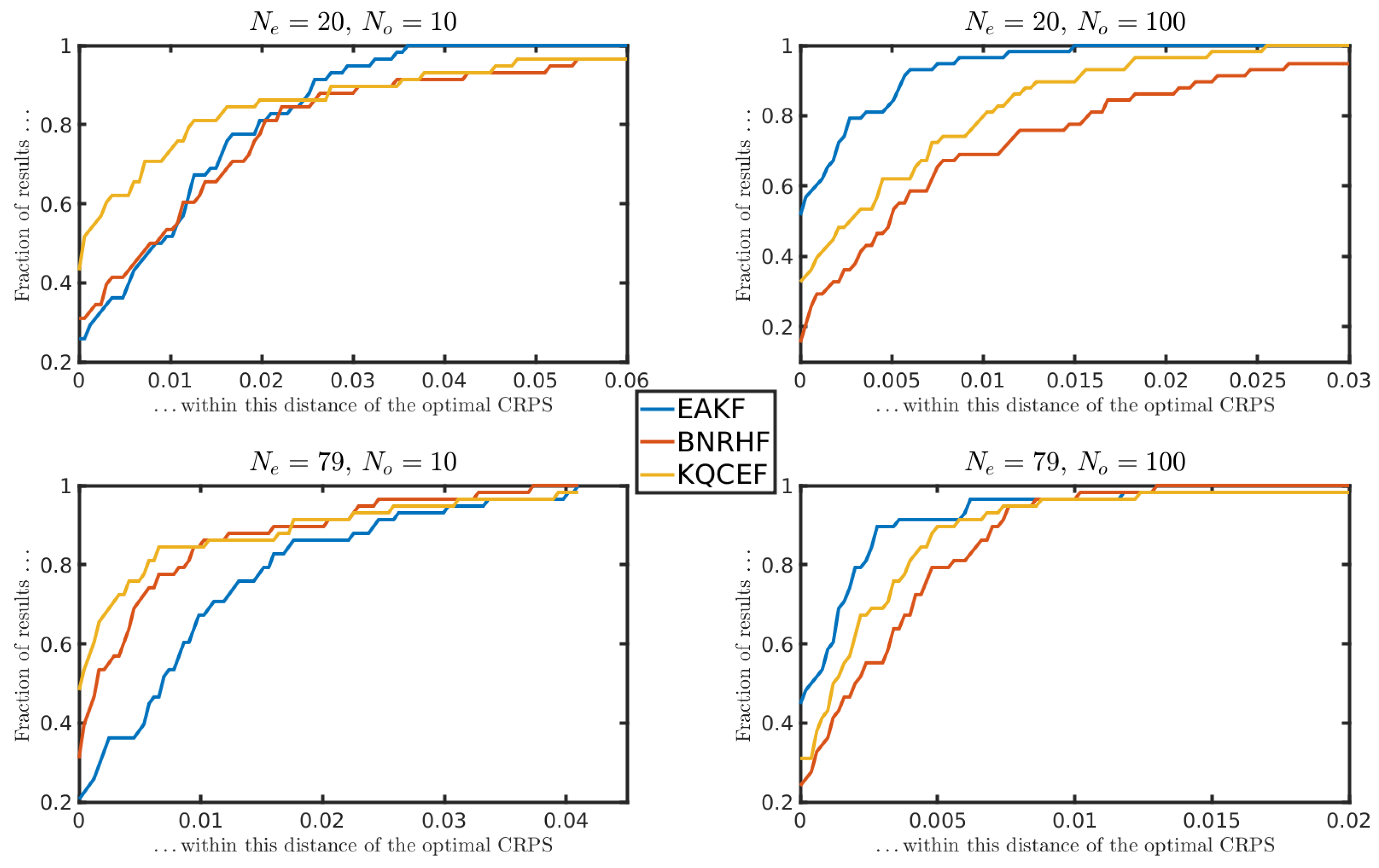
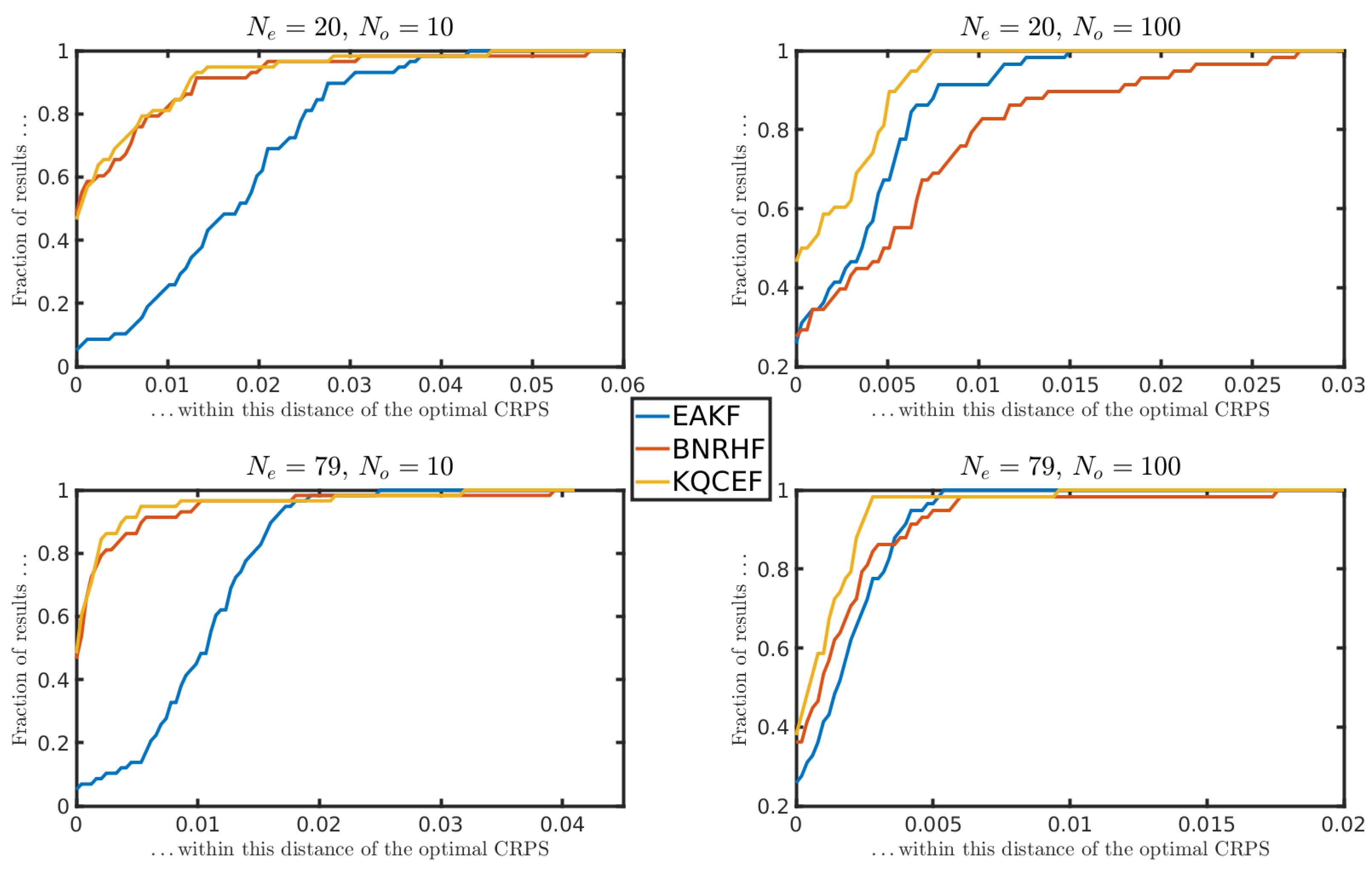
For each experimental configuration, we effectively had assimilation cycles on 58 different days. On some days, EAKF outperforms the other two filters. On other days, BNRHF outperforms the other two. To meaningfully compare these filters, we use a performance profile plot. Each panel of Figure 9 corresponds to a different combination of ensemble size and observation number . The left edge of the panel shows, for each filter, the fraction of the time that it achieved the best CRPS out of the three filters. For example, in the upper left panel (, ), the KQCEF produced the best analysis CRPS about 40% of the time, while the EAKF and BNRHF each produced the best CRPS about 30% of the time. Naturally, it does not mean much to be second-best (or third-best) if the difference between the results is small. The performance plot takes this into account by adding a tolerance. In the same panel (, ), if we look at the value on the horizontal axis, we see that the analysis CRPS produced by the KQCEF was within 0.01 of the best result of about 70% of the time, while the EAKF and BNRHF were both within 0.01 of the best CRPS about 50% of the time. The left side of each panel shows how often each filter is close to the optimal filter. The right side of the panel shows how often each filter is far from optimal.
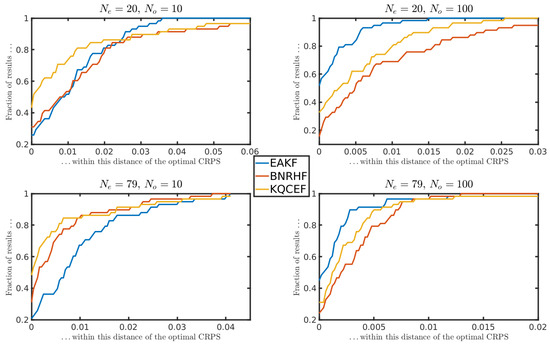
Figure 9.
Analysis CRPS performance profiles, as described in the text.
4.3.1. Analysis
The results of Figure 9 can be summarized as follows. The upper left panel shows that when the observation error variance is relatively large (), and the ensemble is small (), the KQCEF analysis is usually close to optimal. EAKF is slightly more robust in the sense that the analysis CRPS produced by EAKF is always within about 0.35 of the best overall, whereas the analysis CRPS produced by KQCEF is sometimes farther from optimal. In this panel, BNRHF performs the worst of the three filters.
The lower-left panel shows that when the observation error variance is relatively large () and the ensemble is large (), the BNRHF and KQCEF are similar to each other, and both better than EAKF. Both of the right panels show that when the observation error variance is relatively small (), the EAKF is better than the KQCEF, which is better than the BNRHF. In these right panels, the overall CRPS values are small, though, so all three filters are performing well overall.
There is an apparent contradiction between the results shown here for small observation error variance and the results from Section 3. Here, the EAKF outperforms the other filters when the observation error variance is small (large ) and the ensemble size is large, whereas in Section 3.2, the ranking was KQCEF (best), EAKF, BNRHF (worst). These results can be reconciled by noting the different ways in which performance is measured in these experiments. In Section 3.2, the null hypothesis might be rejected because the analysis ensemble has the wrong shape despite being closely centered on the true value, whereas in this section, performance is measured using CRPS, which is small when the analysis ensemble is tightly clustered about the true state.
4.3.2. Forecast
Figure 10 is the same as Figure 9 except that Figure 10 shows the CRPS for the ensemble forecast on the 10th day, i.e., at the longest lead time, when the errors are largest. The left panels of Figure 10 show that when the observation error variance is relatively large (), the BNRHF and KQCEF both perform similarly and are both significantly better than the EAKF. The right panels show that the KQCEF is the best filter for small observation error variance (), though the difference compared to the other two filters is reduced at larger ensemble sizes.
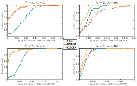
Figure 10.
Forecast CRPS performance profiles, as described in the text.
These results tell a slightly different story than the analysis CRPS results; in particular, the EAKF is never the best filter overall when considering forecast CRPS. In particular, although the EAKF produces the best analysis when the observation error variance is small, the analysis ensemble error grows faster for the EAKF than for the other filters so that KQCEF produces a better forecast.
5. Discussion
We have introduced a new approach, based on kernel-density estimation and quadrature, to approximate the CDF and quantile function needed to implement a QCEF. Previous QCEFs include the Rank Histogram Filter and Bounded Normal Rank Histogram Filter [6,7,8] and the improved Rank Histogram Filter (iRHF [4]). The iRHF also used kernel-density estimation; the approach developed here improves on the iRHF using a quadratic kernel rather than a piecewise-constant kernel by enabling treatment of bounded distributions, enabling treatment of mixed distributions with nonzero total probability on the boundaries, and using quadrature to approximate the CDFs (whereas the iRHF interpolated the likelihood function and then integrated analytically).
The results of Section 3.1 show that nonparametric QCEFs like the BNRHF and KQCEF do not improve on EnKFs when the underlying distributions are Gaussian. Not only do they not improve, but they can, in fact, perform worse than the EAKF: Both BNRHF and KQCEF perform worse than EAKF when the observation is in the tail of the prior, and BNRHF also performs worse than EAKF when the observation error variance is much smaller than the prior variance. This is an example of a broader principle that filters based on parametric distributions—e.g., ensemble Kalman filters and filters based on Gamma and Inverse Gamma distributions [19]—should be expected to outperform their nonparametric counterparts whenever the forecast and likelihood approximately match the assumptions of the parametric filters.
On the other hand, the results of Section 3.2 and Section 3.3 show that BNRHF and KCQEF perform significantly better than EAKF in non-Gaussian problems, as expected. In these problems, the KQCEF performs significantly better than BNRHF, especially when the observation error variance is small compared to the prior variance. The treatment of mixed distributions by KQCEF was shown to be better than BNRHF in Section 3.3, but this could be easily amended within the implementation of BNRHF. One potential advantage of BNRHF over KQCEF that was not explored here is that KQCEF can only handle mixed distributions with delta distributions on the boundaries, whereas BNRHF can accommodate delta distributions anywhere within the distribution [8]. A significant caveat on the results of Section 3.1, Section 3.2 and Section 3.3 is that the filter performance is quantified using the Kolmogorov–Smirnov test with the null hypothesis that the analysis ensemble is drawn from the known true posterior distribution. This is a stringent test; failing this test does not necessarily imply that the root mean squared error would be high, for example.
We applied EAKF, BNRHF, and KQCEF in an idealized model for data assimilation of satellite observations of sea-ice concentration (SIC). Broadly summarizing the results:
- Both QCEF methods (BNRHF and KQCEF) outperform EAKF when the problem is non-Gaussian,
- KQCEF and BNRHF produce similar results when the ensemble size is large, but KQCEF tends to produce better results than BNRHF when the ensemble size is small, and
- The gap between KQCEF and BNRHF is largest when the ensemble size is small, and the observation error variance is also small compared to the prior variance.
The methods developed here all apply to the first step of the two-step framework for ensemble data assimilation [3]. In the context of sea-ice data assimilation, the first step involves updating the ensemble of values of SIC. The second step, in general, updates all the other variables in the sea-ice model based on the updates to SIC. The experiments performed here use a simple second step that is guaranteed to respect the bounds on thicknesses and areas; the development of improved methods for the second step is a topic of future research.
5.1. Small Ensembles and Small Observation Errors
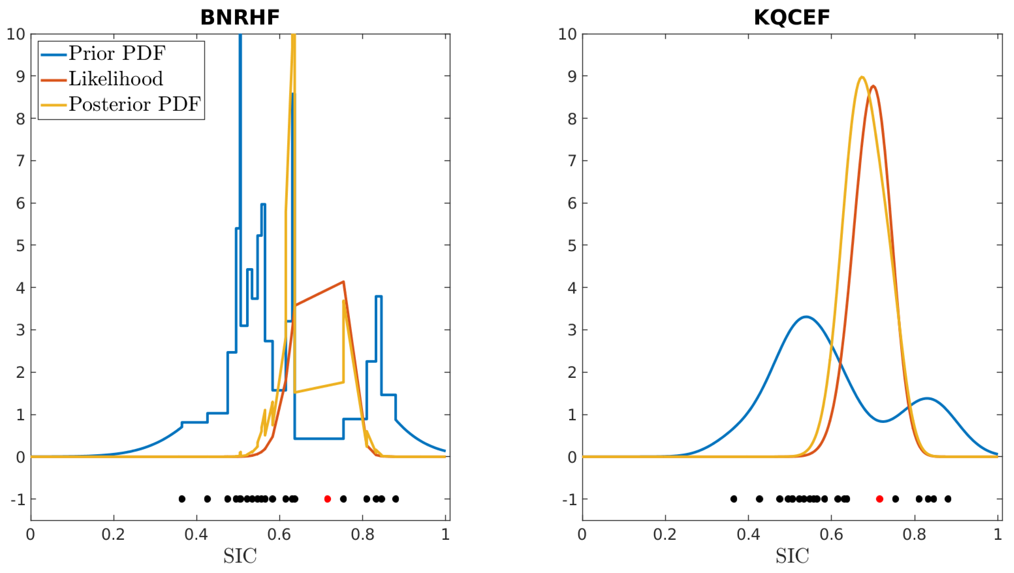
The difference in accuracy between KQCEF and BNRHF when the observation error variance is small compared to the prior variance can be seen in both the idealized tests of Section 3 and Section 4. It can be traced back to the difference in how the likelihood function is treated in the two filters. The BNRHF only evaluates the likelihood function at ensemble members, so if the structure of the likelihood falls mainly between ensemble members, then the BNRHF will not resolve it. In contrast, the KQCEF evaluates the likelihood with infinite resolution, i.e., during the root-finding phase of the algorithm. It evaluates the likelihood wherever needed to obtain an accurate result.
Figure 11 illustrates this using a 20-member ensemble forecast of SIC from the BNRHF filter on 27 September 2011. The BNRHF prior PDF for this ensemble is shown in blue on the left panel, while the KQCEF prior PDF for this same ensemble is shown in blue on the right panel. In both panels, the 20 ensemble members are shown as black dots below the PDFs, and the reference value of SIC is shown as a red dot. The forecast distribution is bimodal, and the reference value lies between the two modes where there are few ensemble members. The red line in the right panel corresponds to the likelihood for and . The KQCEF obtains its posterior PDF by multiplying its prior PDF by the likelihood function (yellow line, right panel). The red line in the left panel evaluates the likelihood of the ensemble members and linearly interpolates between these values. The BNRHF obtains its posterior PDF by multiplying its prior PDF by this linearly interpolated approximation of the likelihood (yellow line, left panel). In this example the reference value (and the peak of the likelihood) is in a trough between two modes of the prior, where there are few ensemble members. Because the BNRHF only evaluates the likelihood at the ensemble members, the peak of the likelihood is not correctly represented, and the BNRHF posterior is incorrect: in this example, the BNRHF posterior PDF is bimodal, with peaks on either side of the reference value. With a larger ensemble, there are fewer gaps, the BNRHF’s piecewise-linear approximation of the likelihood is more accurate, and the result is more accurate.
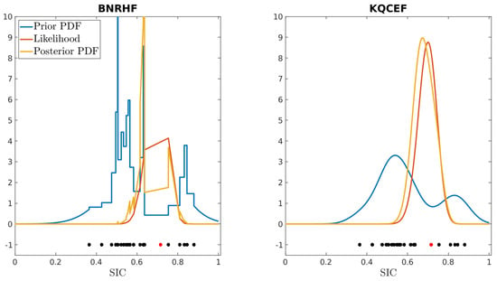
Figure 11.
Forecast (blue) and analysis (yellow) PDFs of SIC for the BNRHF (left) and KQCEF (right) filters. The 20 ensemble members in both plots are drawn from a BNRHF forecast for 27 September 2011; they are shown as black dots beneath the PDFs. The reference value used to generate the observation is shown as a red dot beneath the PDFs. The true likelihood is shown in red in the right panel; it corresponds to an observation with and . The piecewise−linear approximation to the likelihood used by the BNRHF is shown in red in the left panel.
5.2. Forecast vs. Analysis Performance with Icepack
Figure 9 demonstrates that the EAKF outperforms the nonparametric methods when the observation error is small (), yet Figure 10 shows that KQCEF (and sometimes BNRHF) yield better forecasts in these cases. We attempt to explain this mismatch by examining a single analysis/forecast pair.
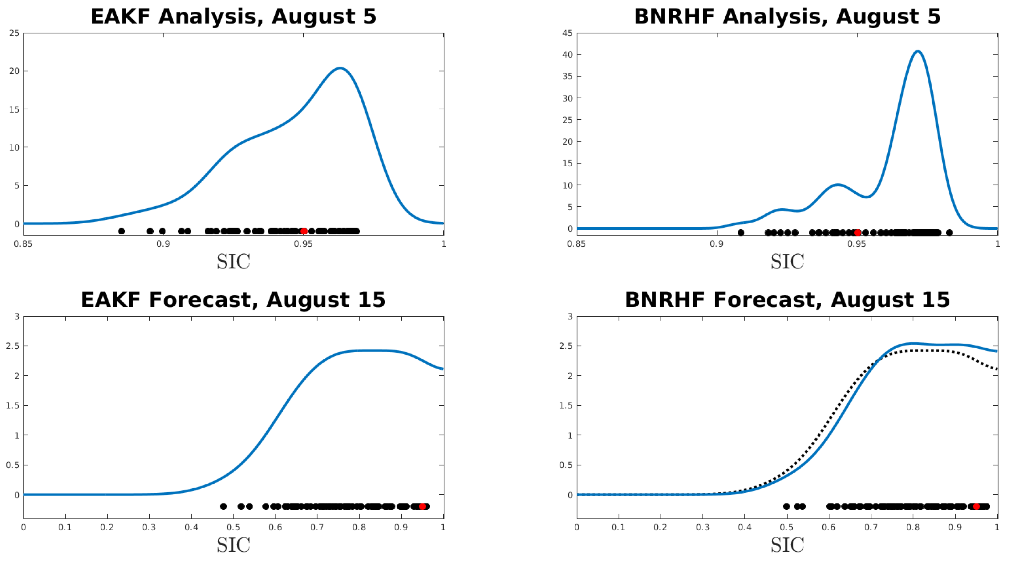
The top row of Figure 12 shows the analysis ensemble (black dots) produced by EAKF (left) and by BNRHF (right) on 5 August 2011; the blue line in each panel is a kernel-density estimate of the analysis PDF, and the red dot shows the reference SIC value. The BNRHF distribution is more tightly centered than the EAKF distribution and is biased high compared to the true SIC value; as a result, the CRPS associated with the EAKF is better (0.0058) than the CRPS associated with the BNRHF (0.0099). Notice that the EAKF produces an analysis ensemble with a longer tail towards low SIC values than the BNRHF. In particular, the smallest ensemble member in the EAKF analysis is noticeably smaller than the smallest ensemble member in the BNRHF analysis.
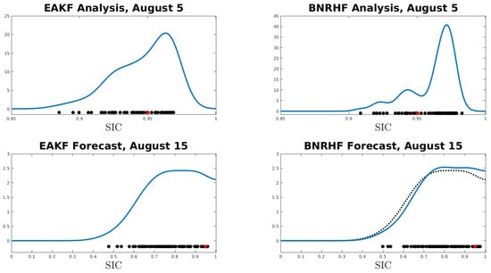
Figure 12.
Top row: Ensemble members (black dots) for the analysis produced by the EAKF (left) and BNRHF (right) on 5 August 2011. Bottom row: Ensemble members (black dots) for the forecast produced by the EAKF (left) and BNRHF (right) on 15 August 2011, initialized from the analysis ensembles shown in the top row. In all panels, the red dot indicates the reference value. The black dotted line in the lower-right panel is the same as the blue line in the lower-left panel, reproduced for ease of comparison.
The bottom row of Figure 12 shows the ensembles (black dots) that result from forecasting the analysis ensembles in the top row 10 days forward to 15 August 2011; the blue line in each panel is a kernel-density estimate of the forecast PDF, and the red dot shows the reference SIC value. The black dotted line in the lower-right panel shows the forecast PDF associated with the EAKF for easier comparison with the forecast PDF associated with the BNRHF (blue). The atmospheric forcing and perturbed parameters of the reference case conspire to keep its SIC value high throughout the 10-day forecast, but the atmospheric forcing and perturbed parameters of the ensemble cause many of the ensemble members to melt out to values of SIC much lower than the reference case. The main difference between the EAKF and BNRHF forecasts is that the EAKF forecast has a longer tail towards low SIC values and has fewer ensemble members close to the large reference SIC value. This results in a larger CRPS for the EAKF forecast (0.0443) compared to the BNRHF forecast (0.0391).
This behavior is common across the time window of interest. The smallest analysis ensemble member produced by the EAKF is almost always significantly smaller than the smallest analysis ensemble members produced by BNRHF and KQCEF across the time window of interest, which is indicative of a longer tail towards low SIC values in the EAKF analysis. This can be traced back to the way in which the filters update the ensemble. The EAKF shifts and scales the ensemble but does not otherwise change its shape. Thus, if the atmospheric forcing and perturbed parameters conspire to create a forecast with a long tail towards small SIC values, the EAKF analysis will also have a tail towards small SIC values. In contrast, both BNRHF and KQCEF change the shape of the ensemble, e.g., moving from a bimodal forecast to a unimodal analysis as shown in the right panel of Figure 11. In this specific context of the Icepack model with perturbed parameters, the result is a poorer performance of EAKF.
5.3. Computational Cost
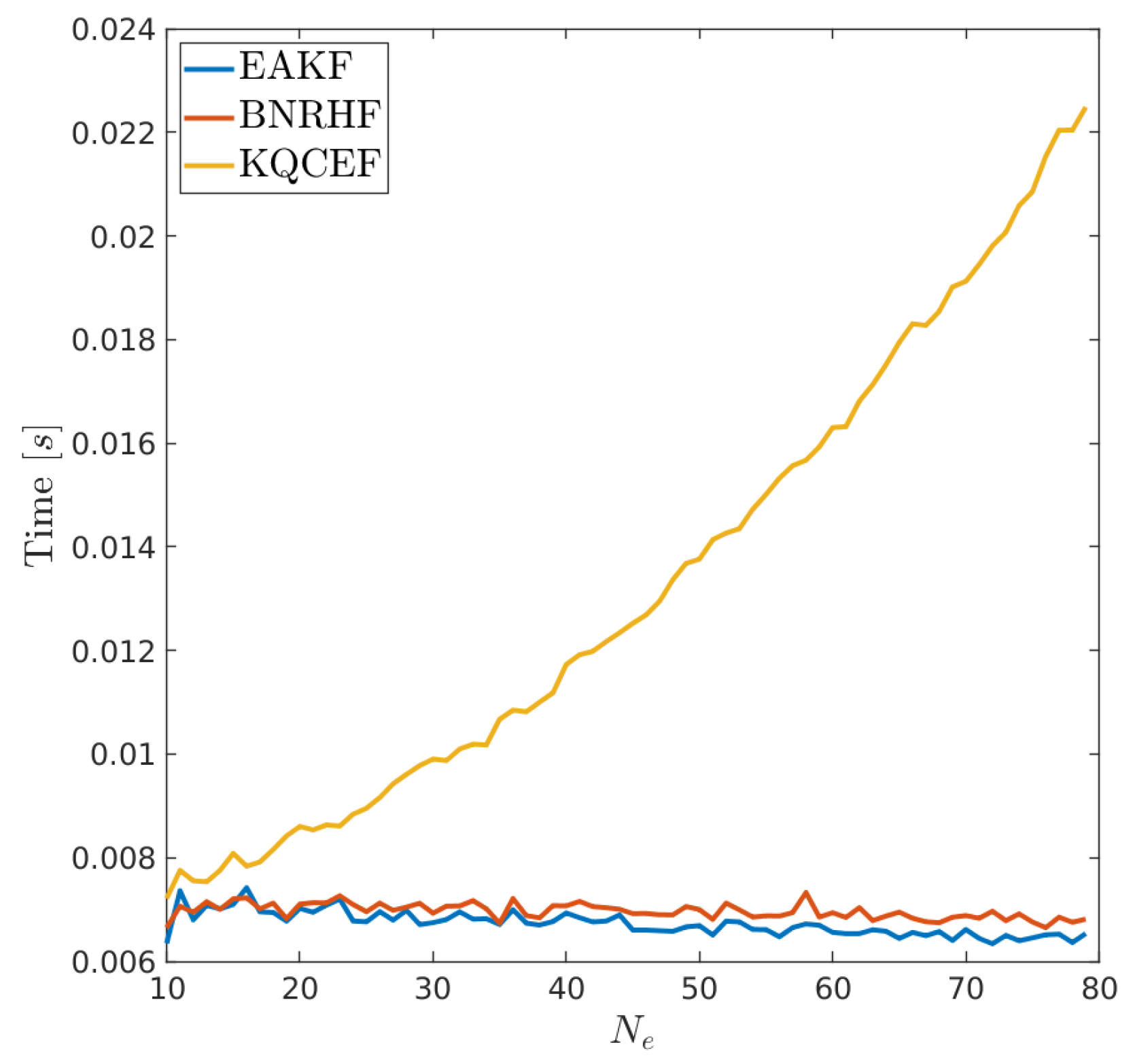
The computational cost of these filters is negligible compared to the forecast step, even when the forecast is an extremely low-cost single-column ice model. On a simple workstation, the forecast step with 79 ensemble members took approximately 8 s. The typical time required to run a single assimilation cycle was computed using the free-running forecast from Figure 8 on 27 September 2011 as the forecast ensemble. The ensemble size was varied from 10 to 79 by selecting the first members of the free-running ensemble. The likelihood used and varied k from 20 through 80. The median time to perform the assimilation was computed across these values of k, and the results are shown as a function of ensemble size in Figure 13. Both EAKF and BNRHF have a total cost approximately independent of ensemble size at a value near 0.007 s per assimilation cycle. The code is not parallelized, so the independence with respect to ensemble size means that the total cost is dominated by overhead costs. KQCEF has a total cost that scales approximately linearly with , which is comparable to the cost of EAKF and BNRHF at and more than three times more expensive at . Even at though, the total cost of the filter is negligible compared to the cost of the ensemble forecast.
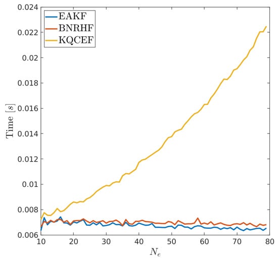
Figure 13.
Median time for a single assimilation cycle for each filter as a function of ensemble size.
The focus here has been on the first step of the two-step framework, i.e., the analysis in observation space. Anderson [7] recently advocated using the bounded normal rank histogram approximation to the prior CDF as part of a generalized linear regression approach to the second step (regression from observation space back to state variables). The KQCEF approximation of the prior CDF could similarly be used in such a context.
The KQCEF has been implemented in DART [46,47] so that it can be available to the data-assimilation research community.
Author Contributions
I.G.: Conceptualization, methodology, software, writing—original draft preparation; C.R.: software, writing—review and editing. All authors have read and agreed to the published version of the manuscript.
Funding
This research was funded by the US National Science Foundation grant number 2152814.
Data Availability Statement
The code and data are available at https://doi.org/10.6084/m9.figshare.25802203.v1 (accessed on 10 June 2024) [48].
Acknowledgments
The authors are grateful to JL Anderson for guidance in implementing KQCEF into DART, and to two anonymous reviewers and Laurent Bertino whose comments led to an improved presentation and discussion of the results.
Conflicts of Interest
The authors declare no conflicts of interest.
Abbreviations
The following abbreviations are used in this manuscript:
| BRNHF | Bounded Normal Rank Histogram Filter |
| EAKF | Ensemble Adjustment Kalman Filter |
| EnKF | Ensemble Kalman Filter |
| KDE | Kernel-Density Estimation |
| KS | Kolmogorov–Smirnov |
| KL | Kullback–Leibler |
| KQCEF | Kernel-based Quantile-Conserving Ensemble Filter |
| QCEF | Quantile-Conserving Ensemble Filter |
Appendix A
Suppose that
is the CDF of a scalar random variable X. Then is a random variable with uniform PDF on :
for . Since the CDF is linear on , the PDF is constant on , which shows that U has a uniform distribution. The derivation above assumes that is invertible in the sense that for every x in the range of X (the first equality), and also that for every (the last equality).
Suppose that U is uniform on and is the CDF of a random variable X. Then the distribution of is the same as the distribution of X:
The last step in this derivation assumes that is a uniformly distributed random variable on . Please note that it does not require for every .
The probability integral transform Equation (1) acts in two steps: First, transform from the prior distribution to a uniform distribution using the prior CDF, then transform to the posterior distribution using the posterior quantile function. What happens when the prior CDF has a jump discontinuity at ? Let the limit from below be
and from above be
If we define for every , then we will be able to satisfy for every x, as long as . But if we define to be any single value in , then we will not be able to satisfy for every . In this case, we cannot directly use Equation (1) to transform from the prior to a uniform distribution.
However, to sample from the posterior distribution, we only need to sample from a uniform distribution and then apply the posterior quantile function. In fact, we could completely skip the first step (transforming from the prior to a uniform) and instead sample from the posterior directly using the posterior quantile function. The problem with such an approach only appears in the second step of two-step ensemble filters, i.e., the step where observation space increments are regressed to state variables. Completely random sampling in observation space scrambles the ensemble increments of the state variables, which can lead to dynamic imbalances.
To avoid this while still making use of the probability integral transform, we need to define a map from the prior (in observation space) to a uniformly distributed random variable. We can achieve this by defining so that is a random variable uniformly distributed on . With this definition, is no longer a deterministic function, but is uniformly distributed on .
The previous analysis focused on mapping from the prior to a uniform distribution when the prior CDF had a jump. What if the posterior CDF has a jump discontinuity at The second step in the transform, from uniform to posterior, does not require for every . It simply requires that is a uniformly distributed random variable on . We can define the CDF as a random map, as above, which satisfies this requirement. From a practical standpoint, this is not necessary since the second step does not actually use the CDF ; it uses the quantile function . It suffices to define for every .
References
- Evensen, G. Sequential data assimilation with a nonlinear quasi-geostrophic model using Monte Carlo methods to forecast error statistics. J. Geophys. Res.-Ocean. 1994, 99, 10143–10162. [Google Scholar] [CrossRef]
- Evensen, G. The ensemble Kalman filter: Theoretical formulation and practical implementation. Ocean Dyn. 2003, 53, 343–367. [Google Scholar] [CrossRef]
- Anderson, J.L. A local least squares framework for ensemble filtering. Mon. Weather Rev. 2003, 131, 634–642. [Google Scholar] [CrossRef]
- Grooms, I. A comparison of nonlinear extensions to the ensemble Kalman filter. Comput. Geosci. 2022, 26, 633–650. [Google Scholar] [CrossRef]
- Anderson, J.L. A Quantile-Conserving Ensemble Filter Framework. Part I: Updating an Observed Variable. Mon. Weather Rev. 2022, 150, 1061–1074. [Google Scholar] [CrossRef]
- Anderson, J.L. A non-Gaussian ensemble filter update for data assimilation. Mon. Weather Rev. 2010, 138, 4186–4198. [Google Scholar] [CrossRef]
- Anderson, J.L. A Quantile-Conserving Ensemble Filter Framework. Part II: Regression of Observation Increments in a Probit and Probability Integral Transformed Space. Mon. Weather Rev. 2023, 151, 2759–2777. [Google Scholar] [CrossRef]
- Anderson, J.; Riedel, C.; Wieringa, M.; Ishraque, F.; Smith, M.; Kershaw, H. A Quantile-Conserving Ensemble Filter Framework. Part III: Data Assimilation for Mixed Distributions with Application to a Low-Order Tracer Advection Model. Mon. Weather Rev. 2024. [Google Scholar] [CrossRef]
- Silverman, B. Density Estimation for Statistics and Data Analysis; CRC Press: Boca Raton, FL, USA, 1998. [Google Scholar]
- Epanechnikov, V.A. Non-parametric estimation of a multivariate probability density. Theory Probab. Its Appl. 1969, 14, 153–158. [Google Scholar] [CrossRef]
- Jones, M.C. Simple boundary correction for kernel density estimation. Stat. Comput. 1993, 3, 135–146. [Google Scholar] [CrossRef]
- Jones, M.; Foster, P. A simple nonnegative boundary correction method for kernel density estimation. Stat. Sin. 1996, 6, 1005–1013. [Google Scholar]
- Atkinson, K. An Introduction to Numerical Analysis; John Wiley & Sons: Hoboken, NJ, USA, 1991. [Google Scholar]
- Oliveira, I.F.; Takahashi, R.H. An enhancement of the bisection method average performance preserving minmax optimality. ACM Trans. Math. Softw. 2020, 47, 1–24. [Google Scholar] [CrossRef]
- Anderson, J.L. An ensemble adjustment Kalman filter for data assimilation. Mon. Weather Rev. 2001, 129, 2884–2903. [Google Scholar] [CrossRef]
- Berger, V.W.; Zhou, Y. Kolmogorov–Smirnov test: Overview. In Wiley Statsref: Statistics Reference Online; John Wiley & Sons: Hoboken, NJ, USA, 2014. [Google Scholar]
- Pérez-Cruz, F. Kullback-Leibler divergence estimation of continuous distributions. In Proceedings of the 2008 IEEE International Symposium on Information Theory, Toronto, ON, Canada, 6–11 July 2008; IEEE: Piscataway, NJ, USA, 2008; pp. 1666–1670. [Google Scholar]
- Bulinski, A.; Dimitrov, D. Statistical estimation of the Kullback–Leibler divergence. Mathematics 2021, 9, 544. [Google Scholar] [CrossRef]
- Bishop, C.H. The GIGG-EnKF: Ensemble Kalman filtering for highly skewed non-negative uncertainty distributions. Q. J. R. Meteorol. Soc. 2016, 142, 1395–1412. [Google Scholar] [CrossRef]
- Morzfeld, M.; Hodyss, D. Gaussian approximations in filters and smoothers for data assimilation. Tellus A Dyn. Meteorol. Oceanogr. 2019, 71, 1600344. [Google Scholar] [CrossRef]
- Grooms, I.; Robinson, G. A hybrid particle-ensemble Kalman filter for problems with medium nonlinearity. PLoS ONE 2021, 16, e0248266. [Google Scholar] [CrossRef] [PubMed]
- Wieringa, M.; Riedel, C.; Anderson, J.A.; Bitz, C. Bounded and categorized: Targeting data assimilation for sea ice fractional coverage and non-negative quantities in a single column multi-category sea ice model. EGUsphere 2023, 2023, 1–25. [Google Scholar]
- Hunke, E.; Allard, R.; Bailey, D.A.; Blain, P.; Craig, A.; Dupont, F.; DuVivier, A.; Grumbine, R.; Hebert, D.; Holland, M.; et al. CICE-Consortium/Icepack: Icepack 1.4.0; CICE-Consortium: Los Alamos, NM, USA, 2023. [Google Scholar] [CrossRef]
- Delworth, T.L.; Broccoli, A.J.; Rosati, A.; Stouffer, R.J.; Balaji, V.; Beesley, J.A.; Cooke, W.F.; Dixon, K.W.; Dunne, J.; Dunne, K.; et al. GFDL’s CM2 global coupled climate models. Part I: Formulation and simulation characteristics. J. Clim. 2006, 19, 643–674. [Google Scholar] [CrossRef]
- Rampal, P.; Bouillon, S.; Ólason, E.; Morlighem, M. neXtSIM: A new Lagrangian sea ice model. Cryosphere 2016, 10, 1055–1073. [Google Scholar] [CrossRef]
- Vancoppenolle, M.; Rousset, C.; Blockley, E.; Aksenov, Y.; Feltham, D.; Fichefet, T.; Garric, G.; Guémas, V.; Iovino, D.; Keeley, S.; et al. SI3, the NEMO Sea Ice Engine. 2023. Available online: https://doi.org/10.5281/zenodo.7534900 (accessed on 10 June 2024).
- Lisæter, K.A.; Rosanova, J.; Evensen, G. Assimilation of ice concentration in a coupled ice–ocean model, using the Ensemble Kalman filter. Ocean Dyn. 2003, 53, 368–388. [Google Scholar] [CrossRef]
- Lindsay, R.W.; Zhang, J. Assimilation of ice concentration in an ice–ocean model. J. Atmos. Ocean. Technol. 2006, 23, 742–749. [Google Scholar] [CrossRef]
- Stark, J.D.; Ridley, J.; Martin, M.; Hines, A. Sea ice concentration and motion assimilation in a sea ice-ocean model. J. Geophys. Res.-Ocean. 2008, 113, C05S91-1-19. [Google Scholar] [CrossRef]
- Metref, S.; Cosme, E.; Snyder, C.; Brasseur, P. A non-Gaussian analysis scheme using rank histograms for ensemble data assimilation. Nonlinear Proc. Geoph. 2014, 21, 869–885. [Google Scholar] [CrossRef][Green Version]
- Barth, A.; Canter, M.; Van Schaeybroeck, B.; Vannitsem, S.; Massonnet, F.; Zunz, V.; Mathiot, P.; Alvera-Azcárate, A.; Beckers, J.M. Assimilation of sea surface temperature, sea ice concentration and sea ice drift in a model of the Southern Ocean. Ocean Model. 2015, 93, 22–39. [Google Scholar] [CrossRef]
- Massonnet, F.; Fichefet, T.; Goosse, H. Prospects for improved seasonal Arctic sea ice predictions from multivariate data assimilation. Ocean Model. 2015, 88, 16–25. [Google Scholar] [CrossRef]
- Chen, Z.; Liu, J.; Song, M.; Yang, Q.; Xu, S. Impacts of assimilating satellite sea ice concentration and thickness on Arctic sea ice prediction in the NCEP Climate Forecast System. J. Clim. 2017, 30, 8429–8446. [Google Scholar] [CrossRef]
- Zhang, Y.F.; Bitz, C.M.; Anderson, J.L.; Collins, N.; Hendricks, J.; Hoar, T.; Raeder, K.; Massonnet, F. Insights on sea ice data assimilation from perfect model observing system simulation experiments. J. Clim. 2018, 31, 5911–5926. [Google Scholar] [CrossRef]
- Riedel, C.; Anderson, J. Exploring Non-Gaussian Sea Ice Characteristics via Observing System Simulation Experiments. EGUsphere 2023, 2023, 1–30. [Google Scholar] [CrossRef]
- Abdalati, W.; Zwally, H.J.; Bindschadler, R.; Csatho, B.; Farrell, S.L.; Fricker, H.A.; Harding, D.; Kwok, R.; Lefsky, M.; Markus, T.; et al. The ICESat-2 laser altimetry mission. Proc. IEEE 2010, 98, 735–751. [Google Scholar] [CrossRef]
- Johnson, N.L.; Kotz, S.; Balakrishnan, N. Continuous Univariate Distributions, Volume 2; John Wiley & Sons: Hoboken, NJ, USA, 1995; Volume 289. [Google Scholar]
- Raeder, K.; Hoar, T.J.; El Gharamti, M.; Johnson, B.K.; Collins, N.; Anderson, J.L.; Steward, J.; Coady, M. A new CAM6+ DART reanalysis with surface forcing from CAM6 to other CESM models. Sci. Rep. 2021, 11, 16384. [Google Scholar] [CrossRef] [PubMed]
- Danabasoglu, G.; Lamarque, J.F.; Bacmeister, J.; Bailey, D.; DuVivier, A.; Edwards, J.; Emmons, L.; Fasullo, J.; Garcia, R.; Gettelman, A.; et al. The community earth system model version 2 (CESM2). J. Adv. Model. Earth Syst. 2020, 12, e2019MS001916. [Google Scholar] [CrossRef]
- Urrego-Blanco, J.R.; Urban, N.M.; Hunke, E.C.; Turner, A.K.; Jeffery, N. Uncertainty quantification and global sensitivity analysis of the Los Alamos sea ice model. J. Geophys. Res.-Ocean. 2016, 121, 2709–2732. [Google Scholar] [CrossRef]
- Smith, G.C.; Allard, R.; Babin, M.; Bertino, L.; Chevallier, M.; Corlett, G.; Crout, J.; Davidson, F.; Delille, B.; Gille, S.T.; et al. Polar ocean observations: A critical gap in the observing system and its effect on environmental predictions from hours to a season. Front. Mar. Sci. 2019, 6, 434834. [Google Scholar] [CrossRef] [PubMed]
- Sakov, P.; Counillon, F.; Bertino, L.; Lisæter, K.; Oke, P.; Korablev, A. TOPAZ4: An ocean-sea ice data assimilation system for the North Atlantic and Arctic. Ocean Sci. 2012, 8, 633–656. [Google Scholar] [CrossRef]
- Kimmritz, M.; Counillon, F.; Bitz, C.; Massonnet, F.; Bethke, I.; Gao, Y. Optimising assimilation of sea ice concentration in an Earth system model with a multicategory sea ice model. Tellus A Dyn. Meteorol. Oceanogr. 2018, 70, 1–23. [Google Scholar] [CrossRef]
- Hersbach, H. Decomposition of the continuous ranked probability score for ensemble prediction systems. Weather Forecast 2000, 15, 559–570. [Google Scholar] [CrossRef]
- Gneiting, T.; Raftery, A.E. Strictly proper scoring rules, prediction, and estimation. J. Am. Stat. Assoc. 2007, 102, 359–378. [Google Scholar] [CrossRef]
- Anderson, J.L.; Collins, N. Scalable implementations of ensemble filter algorithms for data assimilation. J. Atmos. Ocean. Technol. 2007, 24, 1452–1463. [Google Scholar] [CrossRef]
- Anderson, J.; Hoar, T.; Raeder, K.; Liu, H.; Collins, N.; Torn, R.; Avellano, A. The data assimilation research testbed: A community facility. Bull. Am. Meteorol. Soc. 2009, 90, 1283–1296. [Google Scholar] [CrossRef]
- Grooms, I. Data for “A Quantile-Conserving Ensemble Filter Based on Kernel Density Estimation”; figshare: Iasi, Romania, 2024. [Google Scholar] [CrossRef]
Disclaimer/Publisher’s Note: The statements, opinions and data contained in all publications are solely those of the individual author(s) and contributor(s) and not of MDPI and/or the editor(s). MDPI and/or the editor(s) disclaim responsibility for any injury to people or property resulting from any ideas, methods, instructions or products referred to in the content. |
© 2024 by the authors. Licensee MDPI, Basel, Switzerland. This article is an open access article distributed under the terms and conditions of the Creative Commons Attribution (CC BY) license (https://creativecommons.org/licenses/by/4.0/).

