Abstract
Satellite-derived bathymetry (SDB) is an effective means of obtaining global shallow water depths. However, the effect of inherent optical properties (IOPs) on the accuracy of SDB under different water quality conditions has not been clearly clarified. To enhance the accuracy of machine learning SDB models, this study aims to assess the performance improvement of integrating the quasi-analytical algorithm (QAA)-derived IOPs using the Sentinel-2 and ICESat-2 datasets. In different water quality experiments, the results indicate that four SDB models (the Gaussian process regression, neural networks, random forests, and support vector regression) incorporating QAA-IOP parameters equal to or outperform those solely based on the remote sensing reflectance (Rrs) datasets, especially in turbid waters. By analyzing information gains in SDB, the most effective inputs are identified and prioritized under different water qualities. The SDB method incorporating QAA-IOP can achieve an accuracy of 0.85 m, 0.48 m, and 0.74 m in three areas (Wenchang, Laizhou Bay, and the Qilian Islands) with different water quality. Also, we find that incorporating an excessive number of redundant bands into machine learning models not only increases the demand of computing resources but also leads to worse accuracy in SDB. In conclusion, the integration of QAA-IOPs offers promising improvements in obtaining bathymetry and the optimal feature selection should be carefully considered in diverse aquatic environments.
1. Introduction
Coastal regions are among the most economically significant ecosystems [1]. Accurate shallow water depth data are essential to marine engineering, maritime economics, and integrated coastal zone management [2] and are vital for research on nearshore marine dynamics [3]. Basically, all marine activities and maritime spatial planning require depth data [4]. Since survey vessels may not operate in very shallow waters, unmanned aerial vehicles (UAVs) equipped with acoustic bathymetric instruments [5] and airborne bathymetric lidars [6,7] offer a precise and effective method for depth measurement. However, while shipborne and airborne bathymetric instruments can provide very precise depth estimations, their spatial coverages are limited to regional scales rather than a global scale [8,9].
Satellite-derived bathymetry (SDB) offers a rapid and efficient provision of high-resolution underwater topographic maps and acts as a valuable complement to traditional bathymetric techniques [10]. The principle of estimating water depths from multispectral satellite images is based on the premise that the light penetration through the water column at different wavelengths is a function of seawater characteristics [11,12], and models are constructed under various observational conditions to interpret the relationship between multi-dimensional feature values and water depth. Many reliable methods for deriving bathymetry have been developed over the past fifty years [13]. For empirical algorithms, earlier approaches to SDB relied on simple but effective mathematical models constructed from differential reflectance across various bands, such as Lyzenga’s linear band combination model [14] and Stumpf’s logarithmic band ratio model [15]. In developing versatile SDB models, machine learning is perceived as an efficacious methodology, leveraging its capacity for fitting to autonomously explore numerical models and proffer optimal solutions [16]. In recent years, various machine learning algorithms, including neural networks [17,18], random forests [19,20,21], and support vector machines [21,22], have been employed in building SDB models.
Conventionally, most of the SDB studies used in situ measured depth data as control (or training) points to construct empirical SDB models, which limited their applications in some remote areas without available in situ data. Many physical-based SDB models that do not rely on in situ data were also proposed [23,24,25,26], but these have the cost that more spectral information is needed. ICESat-2, as the first photon-counting lidar satellite, provides a new means of directly acquiring bathymetric points worldwide in place of in situ bathymetric data. Within the water depths of 30 m, the accuracy of ICESat-2-derived bathymetric points is generally better than 0.6 m [27]. A number of studies have confirmed that ICESat-2 data are compatible with a wide range of hyperspectral and multispectral data sources including Landsat-8, Sentinel-2, Worldview-2, Pleiades-1, and Zhuhai-1 to achieve SDB using only satellite-based datasets [9,28,29,30,31,32,33,34,35,36,37].
Current studies based on empirical algorithms for SDB typically input all available features into machine learning models. In addition to the remote sensing reflectance Rrs that are directly observed by spaceborne optical sensors, some studies also considered the absorption coefficients at specific wavelengths or other inherent optical parameters (IOPs) when training the SDB models [38,39,40]. The absorption and scattering effect of the water column precludes deep penetration of the light and greatly influence the remote sensing reflectance Rrs [41]. In other words, differences in IOPs can lead to significant differences in Rrs even at the same water depth, and thus inputting IOP information can improve the bathymetric accuracy in complex coastal scenarios. However, on one hand, present machine learning studies on SDB are mostly concentrated along coasts or on islands far from urban areas, where the water qualities are very good. The empirical SDB band selection methods established for clear water bodies probably perform poorly in relatively turbid waters [42]. On the other hand, incorporating an excessive number of redundant bands into machine learning models can lead to worse accuracy in SDB and increased computational demand [43]. As a result, identifying the most effective bands under different water quality conditions is well worth investigating. The quasi-analytical algorithm (QAA) is a classic model for IOP retrievals [11], whose accuracy in coastal areas has been verified as reliable in both clear and turbid waters [44,45,46]. Utilizing machine learning models and the QAA algorithm, the effectiveness of input information for SDB models can be evaluated under varying water quality conditions.
This study aims to derive a machine learning SDB model and increase its accuracy by integrating the QAA algorithm, and then quantitatively analyze the most effective input features under different water quality conditions. Specifically, we extract ICESat-2 bathymetric points as ground truth data from three study areas with different water qualities. After preprocessing Sentinel-2 data, we expand the dimensionality of the Rrs dataset from Sentiel-2 to QAA-derived IOPs in different bands. This expansion is then processed by a dimensionality reduction through the wrapper method. Reducing the dimensions of the expanded dataset can be viewed as an evaluation of the most effective input information. We use four machine learning algorithms, i.e., the Gaussian process regression, neural networks, random forests, and support vector regression, to develop their corresponding SDB models. The accuracy and robustness of this new method are subsequently evaluated in three study areas. By assessing information gains, this study presents the information quantities of different features in SDB and gives priority rankings under different water quality conditions.
2. Study Areas and Dataset
Three areas in China are selected with different water qualities (shown in Figure 1). The first area is located in the South China Sea and near the coast of Wenchang [19.7810°N, 111.0021°E]. This coastal area is generally rural with relatively good water quality, which belongs to water type III based on the Jerlov classification [47].
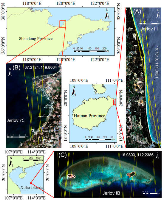
Figure 1.
Location of the three study areas. (A) The basemap for Wenchang is from the image on 21 June 2020; (B) the basemap for Laizhou Bay is from the Sentinel-2 image captured on 9 September 2019; and (C) the basemap for the Qilian Islands is from the Sentinel-2 image captured on 4 April 2023. The yellow lines represent the ICESat-2 ground tracks.
The second area is located in Laizhou Bay [37.2724°N, 119.8064°E] and near the estuary of the Yellow River. This coastal area contains a high sediment load, numerous aquaculture zones and docks, and belongs to water type 7C based on the Jerlov classification. The third area is located in the Qilian Islands [16.9803°N, 112.2386°E] of the South China Sea. This coral reef has very good water quality, which belongs to water type IB based on the Jerlov classification. Figure 1 displays the study area using the Sentinel-2 satellite imagery as the basemap, where the yellow tracks represent the ICESat-2 data used in the experiment. Table 1 lists the details of all the data utilized in this study.

Table 1.
Study area information and Sentinel-2 and ICESat-2 data acquisition time.
2.1. Sentinel-2 Data
The European Space Agency’s (ESA) Copernicus Sentinel-2 mission includes two polar-orbiting satellites carrying the MultiSpectral Instrument (MSI), which provides thirteen available spectral bands. The Sentinel-2 data utilized in this study can be obtained from the European Space Agency (ESA) Sentinel Scientific Data Hub. In this study, we utilize the 10 m resolution bands at 490 nm, 560 nm, and 665 nm, 20 m resolution bands at 865 nm, and 60 m resolution bands at 443 nm. The Sentinel-2 Level-1C top-of-atmosphere reflectance data released by the ESA have undergone geometric correction and radiometric calibration and are geometrically projected in the UTM/WGS84 (Universal Transverse Mercator/World Geodetic System 1984) framework. During the processing of Level-1C datasets to Level-2A, the atmospheric correction is performed using the C2RCC plugin in the SNAP software v9.0.0. Compared to the atmospheric correction by Sen2Cor, C2RCC exhibits better performance in nearshore seawater [35]. Subsequently, the Deglint Operator plugin from the Sen2Cor toolbox is employed for deglint, using NIR (near-infrared) or SWIR (short-wave infrared) to estimate and correct the sun glint in the visible bands. After the above processing, the remote sensing reflectance (Rrs) at 443 nm, 490 nm, 560 nm, 665 nm, and 865 nm are used to construct the SDB dataset. Specifically, the 10 m resolution Rrs at 443 nm and 865 nm are obtained from their 60 m and 20 m resolution Rrs by using the resampling tool in the SNAP software.
2.2. ICESat-2 Data
The payload on ICESat-2 has six laser beams aligned along its trajectory and the cross-track distance is 3.3 km between adjacent beam pairs. A beam pair consists of two laser beams, i.e., the strong beam has a pulse energy that is approximately four times stronger than that of the weak beam. The ICESat-2 Level-2 ATL03 Geolocated Photons product, sourced from https://search.earthdata.nasa.gov/search, accessed on 1 July 2023, is used in this study. The Level-2 ATL03 dataset includes all geolocated photons (including both signal and noise photons) along six tracks (three strong beams and three weak beams). Each photon possesses a unique latitude, longitude, and elevation on the WGS84 ellipsoid reference. Corrections have been conducted to the dataset for the atmospheric delay, solid earth tides, and system pointing biases. However, bathymetry errors caused by surface water fluctuations, instantaneous sea surface heave, etc., are not removed, and this part of the error correction will be introduced in Section 3.
3. Methods
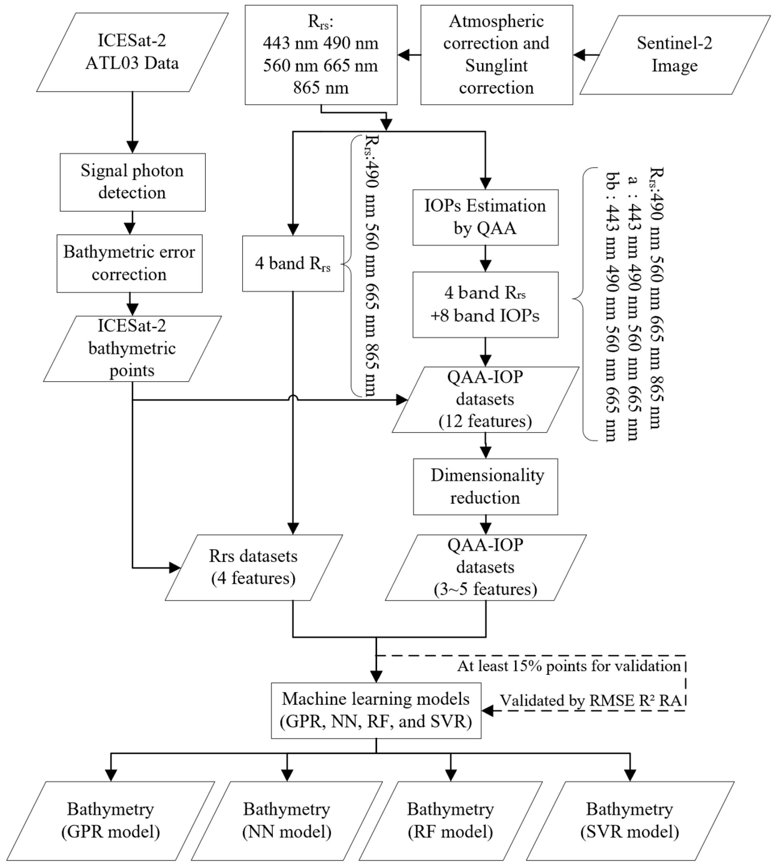
In this study, we employ the density-based spatial clustering of applications with noise (DBSCAN) method to extract surface and bottom photons from ATL03 data and correct the bathymetric errors for the bottom photons. For Sentinel-2 data, by applying the quasi-analytical algorithm (QAA) for four visible light bands of Sentinel-2, the dimensionality of the dataset is expanded to twelve channels. To minimize information redundancy and enhance the efficiency of machine learning models, the wrapper method is then applied to reduce the data dimensionality. Combining the bathymetric points from ICESat-2 and multiple spectral information from Sentinel-2, four machine learning algorithms are utilized to obtain the SDB. To compare and assess the improvement with and without incorporating IOPs, four machine learning models are separately trained using the IOPs+ Rrs dataset or only using Rrs. The effectiveness of these models was evaluated by comparing them with the bathymetric results from ICESat-2. The machine learning techniques used included Gaussian process regression (GPR), neural network (NN), random forest (RF), and support vector regression (SVR). The overall workflow is shown in Figure 2.

Figure 2.
Workflow of ICESat-2- and Sentinel-2-derived bathymetry considering the QAA-derived IOP features.
3.1. ICESat-2 Bottom Photon Detection
The ATL03 product includes signal and noise photons, and this study employs the DBSCAN method to detect the bottom signal photons. The fundamental assumption of DBSCAN denoising is that the density of signal photons is spatially higher than that of noise photons. Specifically, every 10,000 continuous geolocated photons are segmented in the along-track distance. Within each segment, the cluster density of each photon is evaluated as signal if the photon number exceeds the minimum threshold MinPts with a given radius Ra. To prevent the misidentification of solar background noise as signal in the daytime, Ra for daytime data is set as 1.5 m, whereas for nighttime data, it is set as 2.5 m. The minimum threshold MinPts is adaptively calculated as
where SN1 represents the expected number of signal and noise photons within a cluster, while SN2 indicates the expected number of noise photons in the water column [48]. Normally, the vertical layer with the lowest elevation does not include seabed reflection signals, but only contains water backscatter and background noise.
Using the DBSCAN method, sea surface and bottom signal photons are detected from the ATL03 geolocated photons and manually processed to further discard possible noise photons. Then, the bathymetric errors of bottom photons need further correction. In this study, we consider and correct the effects of the water column refraction and forward scattering, sea surface refraction, and sea surface undulations [27,30,35,49]. For each bottom photon, the average elevation of nearby sea surface photons is taken as the instantaneous mean sea surface level, which is then subtracted from the elevation of current bottom photon to determine the instantaneous water depth at that moment. Next, the FES2014 model is used to compensate for water depth variations due to the tidal effect [50,51]. Following the aforementioned procedures, the water depths from the ICESat-2 bathymetric points are obtained.
3.2. QAA for Sentinel-2
In coastal areas, especially near urban areas, water color varies widely by region. Using only remote sensing reflectance for bathymetry may be unreliable due to the significant differences in IOPs. The QAA is a semi-analytical model that adopts the bio-optical model proposed by Lee et al. [11], which calculates the IOPs such as the total absorption (a) and particle backscattering coefficient (bbp) for various wavelengths using multiple spectral reflectance. Utilizing the QAA provides extra IOP parameters for bathymetry. In the latest version of QAA_v6, the central wavelengths of the two reference bands are 555 nm and 665 nm. In this study, we approximate the bands of 555 nm and 670 nm to that of 560 nm and 665 nm, whose Rrs are provided by the MSI sensor. The reliability of the above substitution has been extensively validated [28,29,30]. The wavelengths used in the QAA are 443 nm, 490 nm, 560 nm, and 665 nm. The 10 m resolution images at 443 nm and 865 nm are resampled by the SNAP software.
QAA_v6 estimates a and bbp in all other bands by selecting a reference band λ0, which can be expressed as
aw and bbw are the IOPs of pure seawater and are fixed constants. The coefficients of u and η can be calculated in the QAA_v6 equations, which provides the detailed and complete version of the formula and empirical coefficients. For the reference band λ0, in relatively turbid and clear waters, two different empirical formulas are selected by the magnitude of Rrs(665) in this study in place of Rrs(670). When Rrs(665) ≥ 0.0015 sr−1, the reference band λ0 is at 665 nm, and a and bbp at λ0 at are defined as
When Rrs(665) < 0.0015 sr−1, the reference band λ0 is at 560 nm, and a, bbp at λ0 are calculated using the Rrs(665), Rrs(560), Rrs(490), and Rrs(443). All computational steps are detailed in the QAA_v6 Equation Table [52]. Following the application of the QAA algorithm, in addition to the original four band Rrs with 10 m resolution, eight IOP features are obtained, which are presented in Table 2.

Table 2.
Features after dataset expansion by QAA.
3.3. Dimensionality Reduction
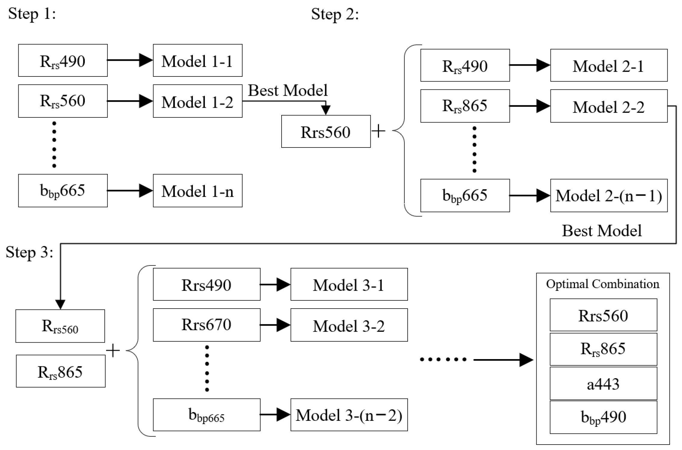
After processing by the QAA algorithm, the Sentinel-2 dataset encompasses 12 features. Some significant autocorrelations may exist among the QAA-derived IOP parameters. Moreover, an excessive number of feature dimensions can lead to an overcomplicated model and reduction in the accuracy of predicted results [43]. As a result, this study utilizes the wrapper method [53] for feature selection to preserve as much of the nonlinear enhancement relationship among IOPs and Rrs at different wavelengths, instead of directly reducing available dimensions using methods like the principal component analysis (PCA). The wrapper method is an iterative feature selection process, which uses the machine learning algorithm to select the optimal subset of features. By choosing the best-performing subset as the starting point for the next iteration, the iterative process continues until a predefined stopping criterion, such as a maximum number of iterations or a certain threshold, is satisfied. The computational process of the wrapper method is depicted in Figure 3.
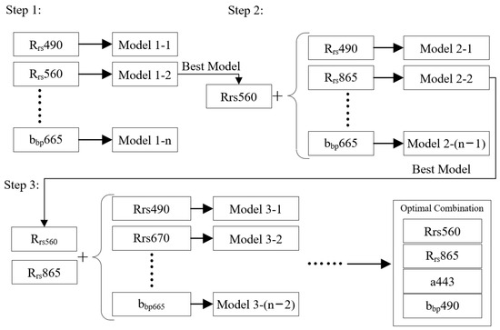
Figure 3.
Schematic of the iterative process of the wrapper method for dimensionality reduction.
In this study, a greedy algorithm is adopted as the search strategy, and the iteration process will terminate when no further decrease is obtained in the residual [54,55]. Clearly, the computational steps involved in the wrapper method can be time-consuming. To reduce the computation time, we choose the random forest algorithm as the iterative model among the four machine learning algorithms introduced in Section 3.4.
3.4. SDB Machine Learning Models
Compared with the classic linear band model and band ratio model [14,15], machine learning algorithms, which are capable of handling nonlinearities, high dimensionality, and potential complex interactive effects, can better model the complex relationships between the water depth and IOP/Rrs features specifically in relatively turbid waters. For bathymetric inversion in this study, we plan to use four types, i.e., the GPR, NN, RF, and SVR.
GPR is a non-parametric model that infers continuous distributions over functions for predictions, utilizing a kernel to define covariances among input data [56]. NN is a computational model, which simulates biological neural networks and learns complex data patterns through interconnected nodes with adjustable weights [57]. RF is an ensemble method employing multiple decision trees to enhance prediction accuracy and control over-fitting by aggregating their outcomes [58]. SVR extends SVM for regression, aiming to minimize deviations from actual targets within a specified margin and ensuring robust predictive performance.
Some hyperparameters need to be set when using these machine learning algorithms. Specifically, for GPR, the shape parameter α is set to 1, the length scale of the kernel l is set to 0.075, and the signal standard deviation is set to 2. For NN, we set the learning rate as 0.01, the momentum parameter as 0.9, the maximum number of iterations as 1000, and the iteration error limit as 1 × 10⁻⁶. For RF, we set the number of learners as 300 and defined the minimum leaf size as 8. For SVR, we utilize the radial basis function (RBF) as the kernel function, setting the kernel scale to 1. The box constraint is defined at 2.324; the epsilon is set at 0.2324; and the data undergoes a standardization.
3.5. Validation Metrics
In this study, we use three metrics, i.e., the root-mean-square error (RMSE), the coefficient of determination (R2), and the mean absolute percentage error (MAPE) to assess the prediction accuracy of the developed model, which are shown in Equations (6)–(8).
where n represents the number of validation points, is the i-th truth depth, is the i-th estimated depth, and is the average truth depth.
4. Results
4.1. Dataset Dimension Reduction and QAA Algorithm Results
As shown in Figure 4, the wrapper method identifies the optimal feature combination for Wenchang as Rrs(560), Rrs(865), a(443), and bbp(490), and these four features compose the QAA-IOP dataset in the study area of Wenchang. It should be noted that multiple combinations of optimal features may exist, which offer an approximately equivalent accuracy, e.g., the combination of Rrs(490), Rrs (865), a(665), and bbp(555) for Wenchang. Near Wenchang, the values of a(443) obtained through the QAA algorithm range from 0.04 to 0.18 m−1, with an average of 0.12 m−1. The values of bbp(490) derived from the QAA algorithm range from 0.005 to 0.025 m−1, with an average value of 0.008 m−1.
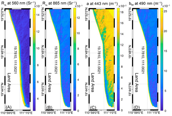
Figure 4.
Optimal feature combination and corresponding Rrs and IOPs results near Wenchang. (A) Rrs result at 560 nm. (B) Rrs result at 865 nm. (C) QAA result of a at 443 nm. (D) QAA result of bbp at 490 nm.
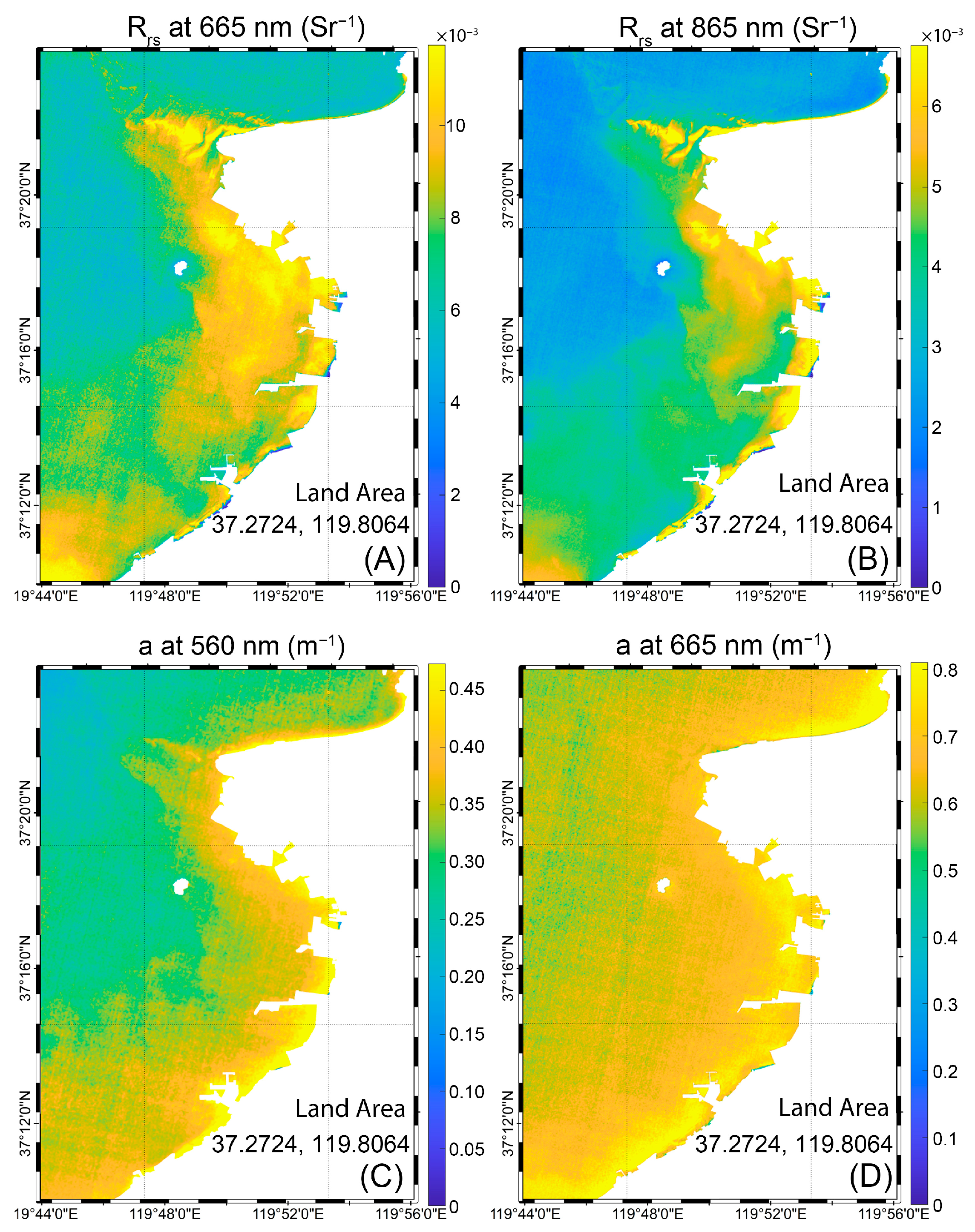
A similar situation exists near Laizhou Bay, where multiple feature combinations could result in comparably precise results. As illustrated in Figure 5, near Laizhou Bay, the optimal feature combination obtained from the wrapper method includes Rrs(665), Rrs(865), a(560), and a(665). Near Laizhou Bay, a(560) ranges from 0.15 to 0.74 m−1 with an average of 0.32 m−1, and a(665) ranges from 0.42 to 0.80 m−1 with an average of 0.65. As shown in Figure 6, the optimal feature combination for the Qilian Islands includes Rrs(490), Rrs(560), Rrs(665), and Rrs(865), which means under this very clear water quality, the performance of the QAA-IOP dataset is equivalent to original Rrs dataset.
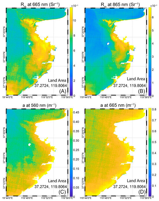
Figure 5.
Optimal feature combination and corresponding Rrs and IOPs results near Laizhou Bay. (A) Rrs result at 665 nm. (B) Rrs result at 865 nm. (C) QAA result of a at 560 nm. (D) QAA result of a at 665 nm.
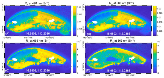
Figure 6.
Optimal feature combination and corresponding Rrs results near the Qilian Islands. (A) Rrs result at 490 nm. (B) Rrs result at 560 nm. (C) Rrs result at 665 nm. (D) Rrs result at 865 nm.
Due to the differences of water types or qualities, the optimal bathymetric inversion combinations can be quite different. As a result, to construct more accurate SDB models, finding the optimal combination of features is recommended which considers the water optical properties in different study areas.
4.2. Results of Different SDB Models and Training Dataset
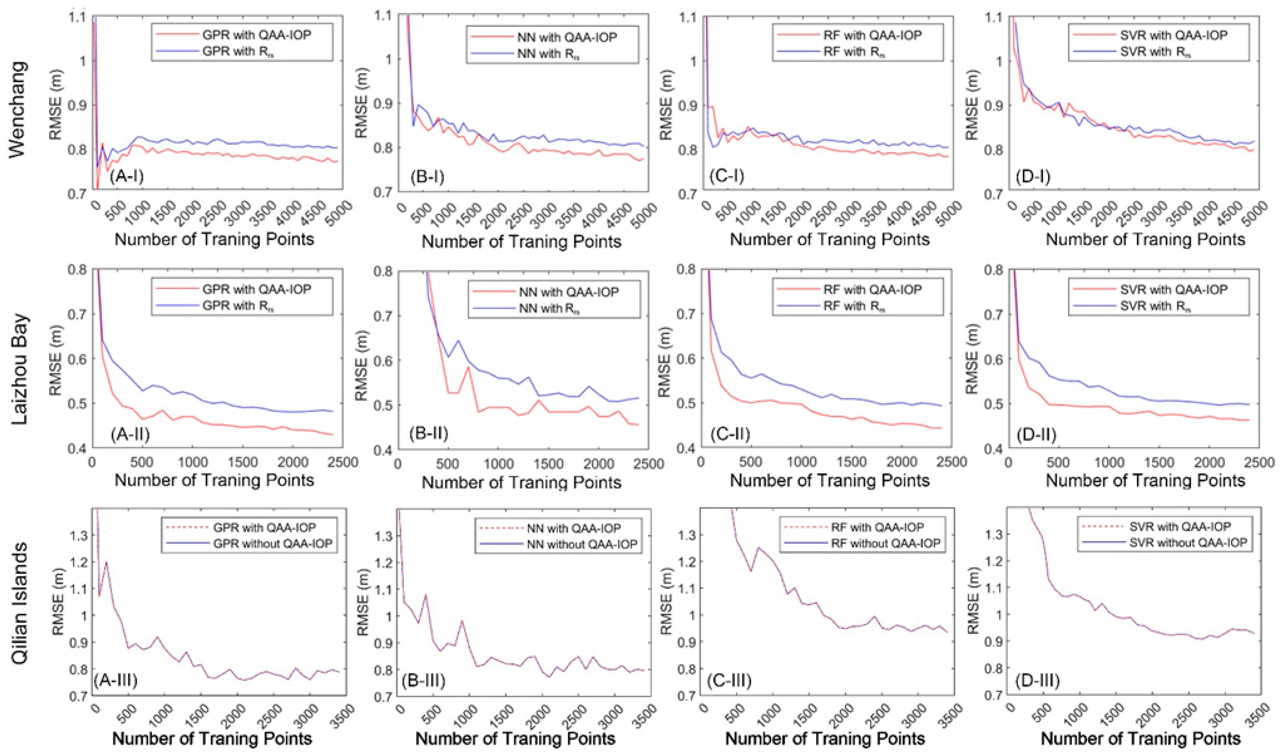
By matching the ICESat-2 bathymetry points with Sentinel-2 imagery, 5312 data pairs are obtained near Wenchang, 2451 pairs near Laizhou Bay, and 3612 pairs near the Qilian Islands. Figure 7 shows how the RMSE of each bathymetry model changes as the number of data training pairs increases. As indicated by the trends in Figure 7, with the exception of the Qilian Islands area, the dataset incorporating QAA-IOP considerably outperforms the dataset with only Rrs, which suggests that the application of QAA-IOP can enhance predictive accuracy and performance, especially in worse water quality or less transparency. Near Wenchang, as the number of training pairs increases to 1000, the GPR and NN algorithms training on the QAA-IOP dataset gradually perform better than that on the Rrs dataset. Notably, the GPR algorithm performs well even with only 1000 training pairs, indicating it may perform better under less data conditions. Near Laizhou Bay, when training pairs reach 500, the accuracy of all four QAA-IOP datasets begin to consistently surpass the four Rrs models. As illustrated in Figure 7C-III,D-III, near the Qilian Islands, the convergence rates of RF and SVR are significantly lower than the other two areas.
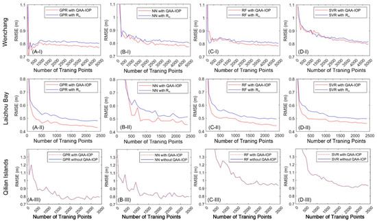
Figure 7.
Training accuracy curves of two datasets using (i.e., NN, GPR, RF, and SVR), with a comparison of with and without QAA-IOP. (A-I–D-I) accrucy curves of four machine learning algorithms of Wenchang. (A-II–D-II) accrucy curves of four machine learning algorithms of Laizhou Bay. (A-III–D-III) accrucy curves of four machine learning algorithms of Qilian Islands. Note that as the performance of the QAA-IOP dataset is identical to the Rrs dataset in the Qilian Islands, the training accuracy curves of the two datasets are overlapped.
Overall, near the Wenchang area, all four models tend to converge around 3500 training pairs, whereas the SVR algorithm may continue to improve with further increments in training pairs. Models near Laizhou Bay tend to converge around 2000 training pairs. Models near the Qilian Islands tend to converge around 3000 training pairs, whereas the RF algorithm may continue to improve with further increments in training pairs. As a result, in subsequent experiments, 3500 pairs are randomly selected and used to train the models for Wenchang and the remaining 2600 pairs are allocated for validation. Near Laizhou Bay, 2000 pairs are randomly selected and used for training and 400 for validation. Meanwhile, near the Qilian Islands, 3000 pairs are selected for training and 600 for validation.
Table 3 lists the performance metrics of the model training and bathymetry validation. Near Wenchang, the GPR, NN, and RF models using the QAA-IOP dataset evidently outperform the models training on the Rrs dataset. Specifically, the GPR and NN models exhibit better performances than the RF and SVR models. Near Laizhou Bay, all four machine learning methods utilizing the QAA-IOP dataset obtain better results than those utilizing the Rrs dataset. Notably, the NN model corresponds to the best performance with the least RMSE (0.44 m and 0.48 m) and largest R2 (0.78 and 0.77) in training and validation, respectively. Near the Qilian Islands, GPR and NN models also exhibit better performances than the RF and SVR models.

Table 3.
Comparison of the model training and validation with the Rrs and QAA-IOP datasets.
In both Figure 7 and Table 3, considering QAA-IOP in Wenchang and Laizhou Bay can improve the model accuracy. Compared to the results in Wenchang, the QAA-IOP dataset has more improvements in all four models near Laizhou Bay, which indicates that the QAA-IOP is more effective in worse water quality or less transparency. In very clear waters, i.e., the Qilian Islands, the performance of the QAA-IOP dataset is identical to the Rrs dataset. Near Wenchang and Laizhou Bay, apart from differences in training and validation accuracy, models that use the Rrs dataset exhibit a slight tendency towards overfitting. For instance, in the GPR model in Wenchang, the training RMSE is 0.85, while the validation RMSE drops to 0.92. Models using the QAA-IOP dataset demonstrate slightly smaller score variations between training and validation sets, suggesting that QAA-IOP might be helpful for reducing overfitting risks. However, to evaluate overfitting risks more precisely, further experiments on larger datasets and detailed model tuning are required.
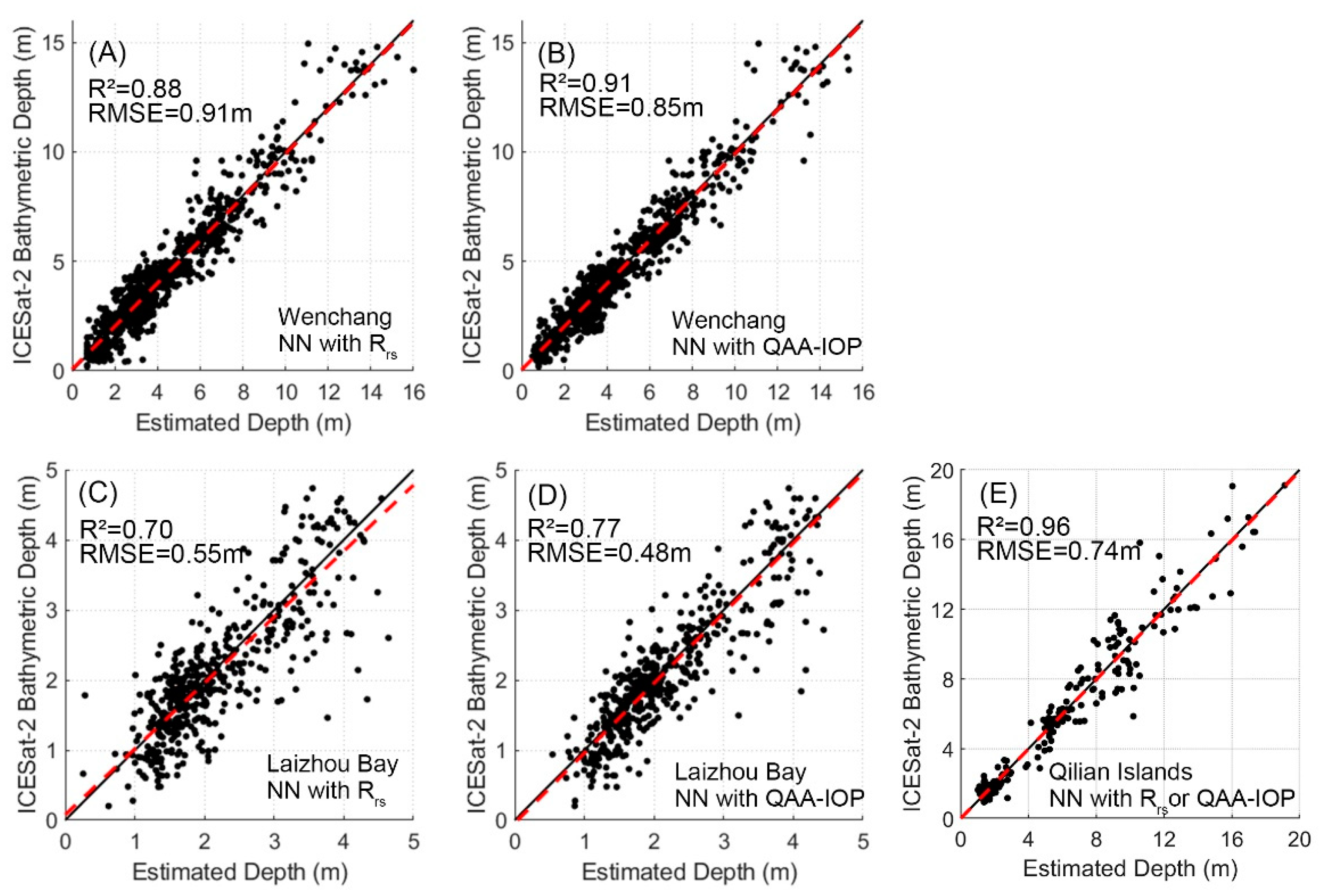
Table 3 demonstrates that the neural network (NN) model exhibits the best accuracy among the four algorithms, and thus the NN model is used to generate bathymetry results in the three study areas. Figure 8 presents a scatterplot of the bathymetry estimations from the NN model against the ICESat-2 validation bathymetric points. In Wenchang, in Figure 8A,B, the maximum depth measured by ICESat-2 is 16 m. Incorporating QAA-IOP parameters significantly reduces the RMSE. For depths less than 10 m, the scatter plots are closely clustered around the reference line of y = x. Due to the limited reference data within the 10–13 m range, a slight accuracy reduction is observed with the QAA-IOP method for these depths.
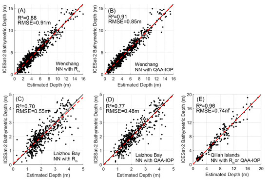
Figure 8.
Bathymetry validations for Wenchang and Laizhou Bay using the NN algorithm. The black solid line represents the 1:1 reference line and the red dashed line represents the regression line. (A) Scatterplot with the Rrs dataset in Wenchang; (B) scatterplot with the QAA-IOP dataset in Wenchang; (C) scatterplot with the Rrs dataset in Laizhou Bay; and (D) scatterplot with the QAA-IOP dataset in Laizhou Bay; and (E) scatterplot with the Rrs or QAA-IOP dataset in the Qilian Islands. Note that the performance of the QAA-IOP dataset is identical to the Rrs dataset in the Qilian Islands.
In Laizhou Bay, in Figure 8C,D, the maximum depth measured by ICESat-2 is only 5 m due to the relatively turbid waters. The worse water quality further introduces lower R2 values than that in Wenchang on both the Rrs and QAA-IOP datasets. Compared to models trained on the Rrs datasets, the accuracy of models incorporating the QAA-IOP parameters is significantly enhanced, with the regression line almost coinciding with the reference line of y = x and error scatter uniformly distributed on both sides of y = x. In the Qilian Islands, in Figure 8E, the maximum depth measured by ICESat-2 is 20 m. Comparing the results in Figure 8A–E, the accuracy of training results on the Rrs dataset in very clear waters is better than that of other water qualities.
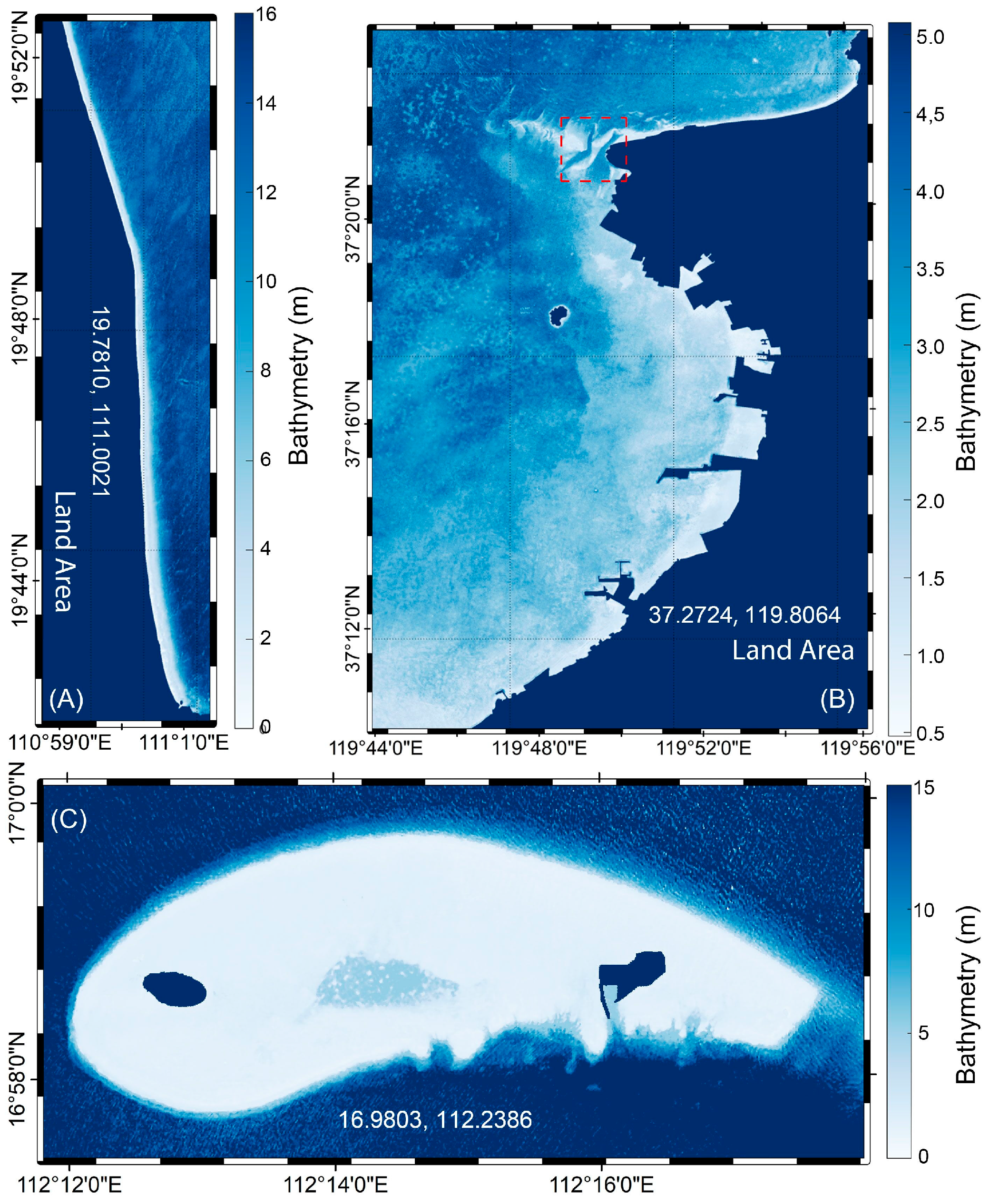
Figure 9 displays the bathymetry maps of Wenchang, Laizhou Bay, and the Qilian Islands generated using the NN models and the QAA-IOP dataset. The bathymetry result in Wenchang indicates that the underwater terrain has many sandy ridges. Near the Yellow River estuary, the bathymetry of Laizhou Bay exhibits a more gradual topographic change. The bathymetry map clearly shows the contours of ridges in the northern part of Laizhou Bay. Furthermore, the navigation channels between Harbor I and Harbor II are distinctly identified within the red dashed box on the Laizhou Bay bathymetry map. The bathymetry result of the Qilian Islands exhibits that the central part of the area is a relatively flat coral reef, with very steep edges around the coral reef. The MAPEs increase as the water qualities worsen in three study areas, i.e., 13.6% in Qilian Islands, 17.5% in Wenchang, and 21.6% in Laizhou Bay.

Figure 9.
Bathymetry from the NN model using the QAA-IOP dataset in Wenchang (A), Laizhou Bay (B), and the Qilian Islands (C). The the red dashed box on Laizhou Bay bathymetry map (B) represents the navigation channels between Harbor I and Harbor II.
5. Discussion
5.1. Error Analysis
In this study, the accuracy of the SDB model is mainly influenced by Sentinel-2 imagery and “truth data” from ICESat-2. The aerosols and sun glint from the Sentinel-2 imagery contribute significantly to the errors in bathymetry [59]. During image preprocessing, the C2RCC algorithm effectively mitigates most of the interference from physical factors on spectral data [60,61]. However, in deeper water areas, uncertainties from atmospheric correction and residual errors from sun glint correction may still introduce discrepancies [62]. In the deeper water regions in Wenchang and the Qilian Islands, regularly shaped error fluctuations are observed, which may be caused by residual errors from sun glint correction. The QAA algorithm in optical shallow waters can be influenced by the high reflectivity of sea bottoms, which further leads to an erroneous estimation of the bottom reflectivity and ultimately manifests as an overestimation of the absorption coefficient [63,64].
Although most scattering and refraction errors in ICESat-2 depth measurements have been corrected, related studies suggest that an approximately 0.4 m bathymetric error still exists in depths less than 30 m [6]. This remaining error is due to the randomness or uncertainty of a photon occurrence, as the bottom signal is normally extremely weak, even less than 0.1 photon on average per shot. Specifically, this uncertainty increases when the width of the detection probability curve broadens, e.g., in more turbid waters or reflected from a bottom with a large slope. Additionally, the uneven distribution of training data pairs in different depth ranges introduces errors in the SDB model [65]. For instance, a notably scarce number of samples exist in Wenchang within the 10–13 m depth range, resulting in significant errors in Figure 8B within this range.
5.2. Variations in the Quantities of Information during Feature Selection Process
When employing the wrapper method to identify the optimal feature combination, multiple equivalent optimal combinations can be found. Taking Laizhou Bay as an example, the optimal combination utilized in this study comprises Rrs(665), Rrs(865), a(560), and a(665). However, alternative combinations, such as Rrs(665), Rrs(865), a(490), a(560), and bbp(665), also achieve nearly identical accuracy levels. To interpret the relationship between the SDB model accuracy and input features, as depicted in Figure 10, we plot the information gains generated by all bands during the SDB process, which is the difference between a certain band and a column of random numbers in conditional entropy [66]. Additionally, we calculate the mutual information among all bands for each area, and the results show that the mutual information between all bands exceeded 0.8. This indicates a very high degree of information overlap among the features.
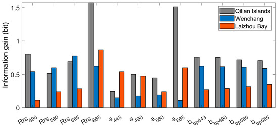
Figure 10.
Information gains provided by all bands during the SDB process.
Based on the information gain and mutual information, it can be inferred that the quantities of information carried by different Rrs and IOPs bands vary. Consequently, a combination of bands, each carrying a lesser quantity of information, can substitute for a single band with a greater quantity of information. Regarding the previously mentioned equivalent combinations for the Laizhou area, the use of a combination of a(490) and bbp(665) achieves the same information content as a(665), which leads to comparable SDB accuracy. Furthermore, for the example of a feature selection iteration process in Laizhou Bay, Rrs(665), Rrs(865), a(490), a(560), and bbp(665) are selected in sequence. As new features are incorporated, the RMSE changed in the following sequence: 0.59, 0.55, 0.51, 0.49, and 0.47 m. It is evident that due to the excessive mutual information, the accuracy improvement experiences diminishing returns. When one more feature (such as a(443)) is further added in the model training, the RMSE even increases to 0.48 m, i.e., the performance gets worse. For machine learning models, reducing data dimensionality may be an effective way to enhance accuracy [43]. Therefore, identifying the most effective bands under different water quality conditions is crucial, rather than inputting all available information into the machine learning model.
As shown in Figure 10, for the Wenchang region that belongs to the Jerlov III water type, the diffuse attenuation coefficient (Kd) is primarily contributed by scattering from water and dissolved particulate matter [47]. Hence, incorporating the particulate backscattering coefficient, such as bbp(490), can effectively improve the accuracy of SDB. In the case of Laizhou Bay, which belongs to the Jerlov 7C water type, the information gains from Rrs at visible wavelengths become significantly lower compared to IOPs. As a result, during the SDB process, the priority of features should be given to the bands that include the effects of Colored Dissolved Organic Matter (CDOM) and chlorophyll, such as a(490) and a(665). For the Qilian Islands, considering IOPs fail to achieve higher SDB accuracy than the Rrs dataset, which may be due to the very clear waters that contain little particles. For regions across all three water quality types, Rrs(856) provides a very high information gain, which might be that the near-infrared (NIR) band supplies essential information for compensating for residuals in the sun glint correction and atmospheric correction.
6. Conclusions
This study presents a new approach to SDB by integrating the QAA with data from the Sentinel-2 and ICESat-2 satellites. With the remote sensing reflectance Rrs from Sentinel-2 and IOPs from QAA as features, we employ ICESat-2 bathymetric data as training data to derive SDB machine learning models. After dimensionality reduction of the features using the wrapper method, we estimate water depths by employing four machine learning models and assess the bathymetric accuracy in three different study areas which correspond to different water qualities.
The results indicate that with the exception of very clear waters (Jerlov IB), incorporating QAA-IOP parameters can significantly enhance bathymetric accuracy, especially in turbid waters. By analyzing information gains in SDB, the most effective inputs are identified and prioritized under different water qualities. Also, incorporating an excessive number of redundant bands into machine learning models not only increases the demand of computing resources but also leads to worse accuracy in SDB. This research evaluates the importance of selecting optimal spectral bands for different water qualities and highlights the potential of machine learning in improving SDB models. Future work should focus on the robustness of these findings across larger datasets and varied coastal environments.
Author Contributions
Conceptualization, Z.L. and Y.M.; methodology, H.L., X.M. and J.Y.; validation, H.L. and Y.J.; writing—original draft preparation, H.L., X.M. and J.Y.; writing—review and editing, Z.L. and S.L.; supervision, Y.M.; funding acquisition, X.M. and Y.M. All authors have read and agreed to the published version of the manuscript.
Funding
This work was funded by the National Natural Science Foundation of China under Grant 42371440, the Key Research and Development Project of Hubei Province under Grant 2022BCA057 and 2021BCA216, the Pre-research Project of Civil Aerospace under Grant D040107, and the Fundamental Research Funds for the Central Universities under Grant 2042023kf0216.
Data Availability Statement
The ICESat-2 ATL03 product can be downloaded from https://search.earthdata.nasa.gov/search (accessed on 1 July 2023), and the Sentinel-2 imagery can be downloaded from https://dataspace.copernicus.eu/browser/ (accessed on 1 July 2023).
Acknowledgments
We sincerely thank the NASA National Snow and Ice Data Center (NSIDC) for distributing the ICESat-2 ATL03 data (https://doi.org/10.5067/ATLAS/ATL03.005), accessed on 1 July 2023, and also thank the ESA’s Sentinel Scientific Data Hub for distributing the Sentinel-2 data (https://doi.org/10.5066/F76W992G), accessed on 1 July 2023.
Conflicts of Interest
The authors declare no conflicts of interest.
References
- Kirwan, M.L.; Megonigal, J.P. Tidal Wetland Stability in the Face of Human Impacts and Sea-Level Rise. Nature 2013, 504, 53–60. [Google Scholar] [CrossRef] [PubMed]
- Brando, V.E.; Anstee, J.M.; Wettle, M.; Dekker, A.G.; Phinn, S.R.; Roelfsema, C. A Physics Based Retrieval and Quality Assessment of Bathymetry from Suboptimal Hyperspectral Data. Remote Sens. Environ. 2009, 113, 755–770. [Google Scholar] [CrossRef]
- Mateo-Pérez, V.; Corral-Bobadilla, M.; Ortega-Fernández, F.; Vergara-González, E.P. Port Bathymetry Mapping Using Support Vector Machine Technique and Sentinel-2 Satellite Imagery. Remote Sens. 2020, 12, 2069. [Google Scholar] [CrossRef]
- Halpern, B.; Walbridge, S.; Selkoe, K.; Kappel, C.; Micheli, F.; D’Agrosa, C.; Bruno, J.; Casey, K.; Ebert, C.; Fox, H.; et al. A Global Map of Human Impact on Marine Ecosystems. Science 2008, 319, 948–952. [Google Scholar] [CrossRef] [PubMed]
- Alvarez, L.; Moreno, H.; Segales, A.; Pham, T.; Pillar-Little, E.; Chilson, P. Merging Unmanned Aerial Systems (UAS) Imagery and Echo Soundings with an Adaptive Sampling Technique for Bathymetric Surveys. Remote Sens. 2018, 10, 1362. [Google Scholar] [CrossRef]
- Su, D.; Yang, F.; Ma, Y.; Wang, X.H.; Yang, A.; Qi, C. Propagated Uncertainty Models Arising From Device, Environment, and Target for a Small Laser Spot Airborne LiDAR Bathymetry and Its Verification in the South China Sea. IEEE Trans. Geosci. Remote Sens. 2020, 58, 3213–3231. [Google Scholar] [CrossRef]
- Tingåker, T.; Ekelund, A. Recent Developments in Airborne LiDAR Bathymetry. In Proceedings of the Electro-Optical Remote Sensing XVI; SPIE: Berlin, Germany, 2022; Volume 12272, pp. 90–99. [Google Scholar]
- Tozer, B.; Sandwell, D.T.; Smith, W.H.F.; Olson, C.; Beale, J.R.; Wessel, P. Global Bathymetry and Topography at 15 Arc Sec: SRTM15+. Earth Space Sci. 2019, 6, 1847–1864. [Google Scholar] [CrossRef]
- Hsu, H.-J.; Huang, C.-Y.; Jasinski, M.; Li, Y.; Gao, H.; Yamanokuchi, T.; Wang, C.-G.; Chang, T.-M.; Ren, H.; Kuo, C.-Y.; et al. A Semi-Empirical Scheme for Bathymetric Mapping in Shallow Water by ICESat-2 and Sentinel-2: A Case Study in the South China Sea. ISPRS J. Photogramm. Remote Sens. 2021, 178, 1–19. [Google Scholar] [CrossRef]
- Hodúl, M.; Bird, S.; Knudby, A.; Chénier, R. Satellite Derived Photogrammetric Bathymetry. ISPRS J. Photogramm. Remote Sens. 2018, 142, 268–277. [Google Scholar] [CrossRef]
- Lee, Z.; Carder, K.L.; Arnone, R.A. Deriving Inherent Optical Properties from Water Color: A Multiband Quasi-Analytical Algorithm for Optically Deep Waters. Appl. Opt. 2002, 41, 5755–5772. [Google Scholar] [CrossRef]
- Lee, Z.; Shang, S.; Hu, C.; Du, K.; Weidemann, A.; Hou, W.; Lin, J.; Lin, G. Secchi Disk Depth: A New Theory and Mechanistic Model for Underwater Visibility. Remote Sens. Environ. 2015, 169, 139–149. [Google Scholar] [CrossRef]
- Kutser, T.; Hedley, J.; Giardino, C.; Roelfsema, C.; Brando, V.E. Remote Sensing of Shallow Waters—A 50 Year Retrospective and Future Directions. Remote Sens. Environ. 2020, 240, 111619. [Google Scholar] [CrossRef]
- Lyzenga, D.R. Shallow-Water Bathymetry Using Combined Lidar and Passive Multispectral Scanner Data. Int. J. Remote Sens. 1985, 6, 115–125. [Google Scholar] [CrossRef]
- Stumpf, R.P.; Holderied, K.; Sinclair, M. Determination of Water Depth with High-Resolution Satellite Imagery over Variable Bottom Types. Limnol. Oceanogr. 2003, 48, 547–556. [Google Scholar] [CrossRef]
- Lee, C.-H.; Liu, L.-W.; Wang, Y.-M.; Leu, J.-M.; Chen, C.-L. Drone-Based Bathymetry Modeling for Mountainous Shallow Rivers in Taiwan Using Machine Learning. Remote Sens. 2022, 14, 3343. [Google Scholar] [CrossRef]
- Liu, S.; Wang, L.; Liu, H.; Su, H.; Li, X.; Zheng, W. Deriving Bathymetry From Optical Images With a Localized Neural Network Algorithm. IEEE Trans. Geosci. Remote Sens. 2018, 56, 5334–5342. [Google Scholar] [CrossRef]
- Collins, A.M.; Geheran, M.P.; Hesser, T.J.; Bak, A.S.; Brodie, K.L.; Farthing, M.W. Development of a Fully Convolutional Neural Network to Derive Surf-Zone Bathymetry from Close-Range Imagery of Waves in Duck, NC. Remote Sens. 2021, 13, 4907. [Google Scholar] [CrossRef]
- Manessa, M.D.M.; Kanno, A.; Sekine, M.; Haidar, M.; Yamamoto, K.; Imai, T.; Higuchi, T. Satellite-Derived Bathymetry Using Random Forest Algorithm and Worldview-2 Imagery. Geoplanning J. Geomat. Plan. 2016, 3, 117. [Google Scholar] [CrossRef]
- Sagawa, T.; Yamashita, Y.; Okumura, T.; Yamanokuchi, T. Satellite Derived Bathymetry Using Machine Learning and Multi-Temporal Satellite Images. Remote Sens. 2019, 11, 1155. [Google Scholar] [CrossRef]
- Duan, Z.; Chu, S.; Cheng, L.; Ji, C.; Li, M.; Shen, W. Satellite-Derived Bathymetry Using Landsat-8 and Sentinel-2A Images: Assessment of Atmospheric Correction Algorithms and Depth Derivation Models in Shallow Waters. Opt. Express 2022, 30, 3238. [Google Scholar] [CrossRef]
- Misra, A.; Vojinovic, Z.; Ramakrishnan, B.; Luijendijk, A.; Ranasinghe, R. Shallow Water Bathymetry Mapping Using Support Vector Machine (SVM) Technique and Multispectral Imagery. Int. J. Remote Sens. 2018, 39, 4431–4450. [Google Scholar] [CrossRef]
- Lee, Z.; Carder, K.L.; Mobley, C.D.; Steward, R.G.; Patch, J.S. Hyperspectral Remote Sensing for Shallow Waters I A Semianalytical Model. Appl. Opt. 1998, 37, 6329. [Google Scholar] [CrossRef] [PubMed]
- Lee, Z.; Carder, K.L.; Mobley, C.D.; Steward, R.G.; Patch, J.S. Hyperspectral Remote Sensing for Shallow Waters: 2 Deriving Bottom Depths and Water Properties by Optimization. Appl. Opt. 1999, 38, 3831. [Google Scholar] [CrossRef] [PubMed]
- Hedley, J.; Roelfsema, C.; Phinn, S.R. Efficient Radiative Transfer Model Inversion for Remote Sensing Applications. Remote Sens. Environ. 2009, 113, 2527–2532. [Google Scholar] [CrossRef]
- Dekker, A.G.; Phinn, S.R.; Anstee, J.; Bissett, P.; Brando, V.E.; Casey, B.; Fearns, P.; Hedley, J.; Klonowski, W.; Lee, Z.P.; et al. Intercomparison of Shallow Water Bathymetry, Hydro-Optics, and Benthos Mapping Techniques in Australian and Caribbean Coastal Environments: Intercomparison of Shallow Water Mapping Methods. Limnol. Oceanogr. Methods 2011, 9, 396–425. [Google Scholar] [CrossRef]
- Parrish, C.E.; Magruder, L.A.; Neuenschwander, A.L.; Forfinski-Sarkozi, N.; Alonzo, M.; Jasinski, M. Validation of ICESat-2 ATLAS Bathymetry and Analysis of ATLAS’s Bathymetric Mapping Performance. Remote Sens. 2019, 11, 1634. [Google Scholar] [CrossRef]
- Xu, N.; Ma, Y.; Zhou, H.; Zhang, W.; Zhang, Z.; Wang, X.H. A Method to Derive Bathymetry for Dynamic Water Bodies Using ICESat-2 and GSWD Data Sets. IEEE Geosci. Remote Sens. Lett. 2022, 19, 1500305. [Google Scholar] [CrossRef]
- Albright, A.; Glennie, C. Nearshore Bathymetry From Fusion of Sentinel-2 and ICESat-2 Observations. IEEE Geosci. Remote Sens. Lett. 2021, 18, 900–904. [Google Scholar] [CrossRef]
- Chen, Y.; Zhu, Z.; Le, Y.; Qiu, Z.; Chen, G.; Wang, L. Refraction Correction and Coordinate Displacement Compensation in Nearshore Bathymetry Using ICESat-2 Lidar Data and Remote-Sensing Images. Opt. Express 2021, 29, 2411. [Google Scholar] [CrossRef]
- Babbel, B.J.; Parrish, C.E.; Magruder, L.A. ICESat-2 Elevation Retrievals in Support of Satellite-Derived Bathymetry for Global Science Applications. Geophys. Res. Lett. 2021, 48, e2020GL090629. [Google Scholar] [CrossRef]
- Le Quilleuc, A.; Collin, A.; Jasinski, M.F.; Devillers, R. Very High-Resolution Satellite-Derived Bathymetry and Habitat Mapping Using Pleiades-1 and ICESat-2. Remote Sens. 2021, 14, 133. [Google Scholar] [CrossRef]
- Xie, C.; Chen, P.; Pan, D.; Zhong, C.; Zhang, Z. Improved Filtering of ICESat-2 Lidar Data for Nearshore Bathymetry Estimation Using Sentinel-2 Imagery. Remote Sens. 2021, 13, 4303. [Google Scholar] [CrossRef]
- Le, Y.; Hu, M.; Chen, Y.; Yan, Q.; Zhang, D.; Li, S.; Zhang, X.; Wang, L. Investigating the Shallow-Water Bathymetric Capability of Zhuhai-1 Spaceborne Hyperspectral Images Based on ICESat-2 Data and Empirical Approaches: A Case Study in the South China Sea. Remote Sens. 2022, 14, 3406. [Google Scholar] [CrossRef]
- Ma, Y.; Xu, N.; Liu, Z.; Yang, B.; Yang, F.; Wang, X.H.; Li, S. Satellite-Derived Bathymetry Using the ICESat-2 Lidar and Sentinel-2 Imagery Datasets. Remote Sens. Environ. 2020, 250, 112047. [Google Scholar] [CrossRef]
- Xu, N.; Ma, X.; Ma, Y.; Zhao, P.; Yang, J.; Wang, X.H. Deriving Highly Accurate Shallow Water Bathymetry From Sentinel-2 and ICESat-2 Datasets by a Multitemporal Stacking Method. IEEE J. Sel. Top. Appl. Earth Obs. Remote Sens. 2021, 14, 6677–6685. [Google Scholar] [CrossRef]
- Xu, N.; Wang, L.; Zhang, H.-S.; Tang, S.; Mo, F.; Ma, X. Machine Learning Based Estimation of Coastal Bathymetry From ICESat-2 and Sentinel-2 Data. IEEE J. Sel. Top. Appl. Earth Obs. Remote Sens. 2024, 17, 1748–1755. [Google Scholar] [CrossRef]
- Chen, B.; Yang, Y.; Xu, D.; Huang, E. A Dual Band Algorithm for Shallow Water Depth Retrieval from High Spatial Resolution Imagery with No Ground Truth. ISPRS J. Photogramm. Remote Sens. 2019, 151, 1–13. [Google Scholar] [CrossRef]
- Li, J.; Knapp, D.E.; Schill, S.R.; Roelfsema, C.; Phinn, S.; Silman, M.; Mascaro, J.; Asner, G.P. Adaptive Bathymetry Estimation for Shallow Coastal Waters Using Planet Dove Satellites. Remote Sens. Environ. 2019, 232, 111302. [Google Scholar] [CrossRef]
- Wu, Z.; Mao, Z.; Shen, W.; Yuan, D.; Zhang, X.; Huang, H. Satellite-Derived Bathymetry Based on Machine Learning Models and an Updated Quasi-Analytical Algorithm Approach. Opt. Express 2022, 30, 16773. [Google Scholar] [CrossRef] [PubMed]
- Kirk, J.T.O. Light and Photosynthesis in Aquatic Ecosystems; Cambridge University Press: Cambridge, UK, 1994; ISBN 978-0-521-45966-2. [Google Scholar]
- Caballero, I.; Stumpf, R.P. Confronting Turbidity, the Major Challenge for Satellite-Derived Coastal Bathymetry. Sci. Total Environ. 2023, 870, 161898. [Google Scholar] [CrossRef]
- Kohavi, R.; John, G.H. Wrappers for Feature Subset Selection. Artif. Intell. 1997, 97, 273–324. [Google Scholar] [CrossRef]
- Qing, S.; Tang, J.; Cui, T.; Zhang, J. Retrieval of Inherent Optical Properties of the Yellow Sea and East China Sea Using a Quasi-Analytical Algorithm. Chin. J. Oceanol. Limnol. 2011, 29, 33–45. [Google Scholar] [CrossRef]
- Pitarch, J.; van der Woerd, H.J.; Brewin, R.J.W.; Zielinski, O. Optical Properties of Forel-Ule Water Types Deduced from 15 years of Global Satellite Ocean Color Observations. Remote Sens. Environ. 2019, 231, 111249. [Google Scholar] [CrossRef]
- Zhan, J.; Zhang, D.J.; Zhang, G.Y.; Wang, C.X.; Zhou, G.Q. Estimation of Optical Properties Using Qaa-V6 Model Based on Modis Data. Int. Arch. Photogramm. Remote Sens. Spat. Inf. Sci. 2020, XLII-3-W10, 937–940. [Google Scholar] [CrossRef]
- Williamson, C.A.; Hollins, R.C. Measured IOPs of Jerlov Water Types. Appl. Opt. 2022, 61, 9951. [Google Scholar] [CrossRef] [PubMed]
- Ma, Y.; Xu, N.; Sun, J.; Wang, X.H.; Yang, F.; Li, S. Estimating Water Levels and Volumes of Lakes Dated Back to the 1980s Using Landsat Imagery and Photon-Counting Lidar Datasets. Remote Sens. Environ. 2019, 232, 111287. [Google Scholar] [CrossRef]
- Yang, J.; Ma, Y.; Zheng, H.; Gu, Y.; Zhou, H.; Li, S. Analysis and Correction of Water Forward-Scattering-Induced Bathymetric Bias for Spaceborne Photon-Counting Lidar. Remote Sens. 2023, 15, 931. [Google Scholar] [CrossRef]
- Carrere, L.; Lyard, F.; Cancet, M.; Guillot, A. FES 2014, a New Tidal Model on the Global Ocean with Enhanced Accuracy in Shallow Seas and in the Arctic Region. In Proceedings of the EGU General Assembly Conference Abstracts, Vienna, Austria, 12–17 April 2015; p. 5481. [Google Scholar]
- Wang, N.; Gao, Y.; Guo, H.; Lu, J. Analysis of Characteristics of Tide and Tidal Current in the East China Seas. J. Phys. Conf. Ser. 2023, 2486, 012039. [Google Scholar] [CrossRef]
- Lee, Z.; Lubac, B.; Werdell, J.; Arnone, R. Update of the Quasi-Analytical Algorithm (QAA_v6)[R/OL]. International Ocean Color Group Software Report. Available online: https://www.ioccg.org/groups/software.html (accessed on 3 April 2013).
- Karagiannopoulos, M.; Anyfantis, D.; Kotsiantis, S.; Pintelas, P. Feature Selection for Regression Problems. Proceedings of HERCMA’07. Available online: https://www.researchgate.net/publication/228084541_Feature_selection_for_regression_problems (accessed on 1 July 2023).
- Shanab, A.A.; Khoshgoftaar, T.M.; Wald, R. Evaluation of Wrapper-Based Feature Selection Using Hard, Moderate, and Easy Bioinformatics Data. In Proceedings of the 2014 IEEE International Conference on Bioinformatics and Bioengineering, Boca Raton, FL, USA, 10–12 November 2014; pp. 149–155. [Google Scholar]
- Wang, H.; Khoshgoftaar, T.M.; Napolitano, A. An Empirical Investigation on Wrapper-Based Feature Selection for Predicting Software Quality. Int. J. Softw. Eng. Knowl. Eng. 2015, 25, 93–114. [Google Scholar] [CrossRef]
- Williams, C.; Rasmussen, C. Gaussian Processes for Regression. In Advances in Neural Information Processing Systems; MIT Press: Cambridge, MA, USA, 1995; Volume 8. [Google Scholar]
- Theory of the Backpropagation Neural Network|IEEE Conference Publication|IEEE Xplore. Available online: https://ieeexplore.ieee.org/document/118638 (accessed on 20 April 2024).
- Random Decision Forests|IEEE Conference Publication|IEEE Xplore. Available online: https://ieeexplore.ieee.org/document/598994 (accessed on 20 April 2024).
- Hedley, J.D.; Roelfsema, C.; Brando, V.; Giardino, C.; Kutser, T.; Phinn, S.; Mumby, P.J.; Barrilero, O.; Laporte, J.; Koetz, B. Coral Reef Applications of Sentinel-2: Coverage, Characteristics, Bathymetry and Benthic Mapping with Comparison to Landsat 8. Remote Sens. Environ. 2018, 216, 598–614. [Google Scholar] [CrossRef]
- Kutser, T.; Vahtmäe, E.; Rohtla, L. Spectral Library of Macroalgae and Benthic Substrates in Estonian Coastal Waters. Proc. Est. Acad. Sci. Biol. Ecol. 2006, 55, 329–340. [Google Scholar] [CrossRef]
- Casal, G.; Monteys, X.; Hedley, J.; Harris, P.; Cahalane, C.; McCarthy, T. Assessment of Empirical Algorithms for Bathymetry Extraction Using Sentinel-2 Data. Int. J. Remote Sens. 2019, 40, 2855–2879. [Google Scholar] [CrossRef]
- Hedley, J.D.; Harborne, A.R.; Mumby, P.J. Technical Note: Simple and Robust Removal of Sun Glint for Mapping Shallow-water Benthos. Int. J. Remote Sens. 2005, 26, 2107–2112. [Google Scholar] [CrossRef]
- Pitarch, J.; Vanhellemont, Q. The QAA-RGB: A Universal Three-Band Absorption and Backscattering Retrieval Algorithm for High Resolution Satellite Sensors. Development and Implementation in ACOLITE. Remote Sens. Environ. 2021, 265, 112667. [Google Scholar] [CrossRef]
- Najah, A.; Al-Shehhi, M.R. Performance of the Ocean Color Algorithms: QAA, GSM, and GIOP in Inland and Coastal Waters. Remote Sens. Earth Syst. Sci. 2021, 4, 235–248. [Google Scholar] [CrossRef]
- Huang, Y.; Yang, H.; Tang, S.; Liu, Y.; Liu, Y. An Appraisal of Atmospheric Correction and Inversion Algorithms for Mapping High-Resolution Bathymetry Over Coral Reef Waters. IEEE Trans. Geosci. Remote Sens. 2023, 61, 4204511. [Google Scholar] [CrossRef]
- Kurniabudi; Stiawan, D.; Darmawijoyo; Bin Idris, M.Y.; Bamhdi, A.M.; Budiarto, R. CICIDS-2017 Dataset Feature Analysis with Information Gain for Anomaly Detection. IEEE Access 2020, 8, 132911–132921. [Google Scholar] [CrossRef]
Disclaimer/Publisher’s Note: The statements, opinions and data contained in all publications are solely those of the individual author(s) and contributor(s) and not of MDPI and/or the editor(s). MDPI and/or the editor(s) disclaim responsibility for any injury to people or property resulting from any ideas, methods, instructions or products referred to in the content. |
© 2024 by the authors. Licensee MDPI, Basel, Switzerland. This article is an open access article distributed under the terms and conditions of the Creative Commons Attribution (CC BY) license (https://creativecommons.org/licenses/by/4.0/).


