Abstract
Anthocyanin can improve the stress tolerance and disease resistance of winter wheat to a certain extent, so timely and accurate monitoring of anthocyanin content is crucial for the growth and development of winter wheat. This study measured the ground-based hyperspectral reflectance and the corresponding anthocyanin concentration at four key growth stages—booting, heading, flowering, and filling—to explore the spectral detection of anthocyanin in winter wheat leaves. Firstly, the first-order differential spectra (FDS) are obtained by processing based on the original spectra (OS). Then, sensitive bands (SBS), the five vegetation indices for optimal two-band combinations (VIo2), and the five vegetation indices for optimal three-band combinations (VIo3) were selected from OS and FDS by band screening methods. Finally, modeling methods such as RF, BP, and KELM, as well as models optimized by genetic algorithm (GA), were used to estimate anthocyanin content at different growth stages. The results showed that (1) among all the models, the GA_RF had incredible performance, VIo3 was the superior parameter for estimating anthocyanin values, and the model GA_RF of FDS data based on VIo3 for the filling stage (Rv2 = 0.950, RMSEv = 0.005, RPDv = 4.575) provided the best estimation of anthocyanin. (2) the first-order differential processing could highlight the degree of response of SBS, VIo2, and VIo3 to the anthocyanin values. The model performances of the FDS were better than that of OS on the whole, and the Rv2 of the optimal models of FDS were all greater than 0.89. (3) GA had optimizing effects on the RF, BP, and KELM, and overall, the GA models improved the R2 by 0.00%-18.93% compared to the original models. These results will provide scientific support for the use of hyperspectral techniques to monitor anthocyanin in the future.
1. Introduction
Anthocyanin is a water-soluble natural pigment that belongs to flavonoids [1], existing in winter wheat as a primary color-presenting substance. Anthocyanin has a specific antioxidant effect [2], which can protect winter wheat from oxidative damage. Increasing its value can improve stress tolerance and disease resistance and promote the growth and development of winter wheat [3]. However, a decrease in its value will cause impaired photosynthesis, decreased antioxidant capacity, and weakened stress tolerance in winter wheat, leading to growth and development limitations. Therefore, maintaining punctual information about anthocyanin is significant for monitoring winter wheat growth.
Nevertheless, the traditional methods used for measurements of anthocyanin values, such as high-performance liquid chromatography [4], spectrophotometry [5], and colorimetry [6], require sample crushing in the laboratory. These methods are not only cumbersome and costly but cannot realize real-time monitoring and rapid monitoring of large areas of vegetation [7,8]. Therefore, finding new effective methods for anthocyanin measurements is of great necessity.
In recent years, hyperspectral remote sensing technology has been developing rapidly. With its high efficiency, rapidity, non-invasiveness, and wide range of monitoring abilities, it has gradually become an effective means for quickly monitoring the physicochemical composition of crops in the field. At present, hyperspectral remote sensing technology has achieved promising results in the research of the physicochemical composition of crops, such as nitrogen content [9], chlorophyll content [10], water content [11], and aboveground biomass [12]. It has also been successfully applied in the inversion study of anthocyanin content. For example, Luo et al. [13] used spectral principal components, “three-edge” parameters, and absorption parameters to construct models to estimate the anthocyanin values in peony leaves, respectively, after acquiring the ground hyperspectral data, in which the optimal spectral conversion method and the optimal accuracy model were obtained by comparison. Jiang et al. [14] used hyperspectral data to estimate the anthocyanin values of maize leaves by utilizing sensitive bands, classical vegetation indices (VIs), or optimized VIs as model variables, and it was found that tasseling and lactation stages were more effective for anthocyanin estimation. Gutiérrez et al. [15] used hyperspectral imaging for non-destructive measurement of anthocyanin concentration in wine grapes by training support vector machines, and the cross-validated R2 result reached 0.72, which indicated that hyperspectral imaging for assessing anthocyanin in grapes is promising. By analyzing the above studies, previous researchers have achieved promising results in converting anthocyanin values with SBS and VIs as input variables. However, how to make the input variables work best remains to be explored. The band screening methods (BSM), with their advantages of retaining sensitive spectral information and reducing data redundancy, undoubtedly provide a feasible direction.
To better extract helpful information for research objectives in complex spectra, scholars have applied BSM to research and gained practical experience. Among them, BSMs are mainly used to find SBS and vegetation indices for optimal band combinations (VIo) [16,17,18]. In existing studies, successive projections algorithm (SPA) [19], competitive adaptive reweighted sampling (CARS) [20], uninformative variable elimination (UVE) [21], iteratively retaining informative variables (IRIV) [22], and many other methods have been used for extracting SBS. Although individual selection methods are effective, some studies have shown that a combination of the above methods is more capable of selecting suitable SBS and improving model accuracy [23,24]. For instance, Liang et al. [25] found that the CARS-IRIV algorithm could effectively reduce the number of variables extracted by the CARS algorithm and stabilize the model prediction accuracy in a study on the rapid detection of soluble solids content in “Korla balsam pears”. Zhang et al. [26] used the CARS algorithm to filter the twenty-eight feature bands selected by the SPA algorithm that may contain noise and obtained nine more appropriate feature bands, which in turn constructed the XGboost as the best model for inverting winter wheat LAI. Moreover, it has been shown that using VIo has achieved favorable outcomes in hyperspectral inversion. Fang et al. [27] respectively screened five VIo3 (ESI, MCARI, SIPI, TSI, NSI) based on OS, FDS, and second-order differential data, using hyperspectral data of Spartina alterniflora, which captured the vegetation information that could not be covered by the traditional VIs and improved the sensitivity of the VIs to LAI. Deng et al. [28] searched for the optimal combination of bands for VIs in a study that used hyperspectral to assess wheat stripe rust. Then, they found that proper multi-VIo modeling improves the performance compared to single-VIo modeling.
Meanwhile, with the development of artificial intelligence technology, several machine learning (ML) algorithms have been applied to monitor biochemical parameters in winter wheat [29,30]. However, the performance of machine learning models (MLs) may be significantly affected by the type and quality of input variables or the number of spectral features [31,32,33,34], especially when the growth health of winter wheat is under stress [35,36]. Hence, choosing appropriate feature BSM and MLs is vital for predicting anthocyanin values of the winter wheat. So far, studies have yet to use the combination of IRIV and SPA for extracting SBS and thus predicting anthocyanin values of winter wheat. Besides, a few studies have explored the selection of band combinations under the range of bands for each factor in the formulas for VIs that are most suitable for the study targets to form an optimal vegetation index, predicting winter wheat anthocyanin values.
In this paper, based on the hyperspectral reflectance of winter wheat leaves in the 350–1000 nm range, IRIV and SPA methods were combined to extract SBS, and VIo was found based on the principle of the maximum correlation coefficient. Then, three MLs and three corresponding GA_MLs were constructed with SBS, VIo2, and VIo3 as input variables for estimating the values of anthocyanin in winter wheat leaves, respectively. The research objectives of this paper were (1) to compare the performance of all models and to investigate the potential of MLs(SBS) and MLs(VIo) for estimating anthocyanin values at four fertility stages of winter wheat; (2) to analyze the effect of FDS on the input variables SBS and VIo for estimating anthocyanin values in winter wheat, and to dissect the accuracy of anthocyanin prediction model and its influencing factors; (3) to Analyze the optimization effect of genetic algorithm on the model. The results of this study will provide some technical support for the potential application of hyperspectral technology in detecting and diagnosing anthocyanin in winter wheat.
2. Materials and Methods
2.1. Overview of the Experimental Design
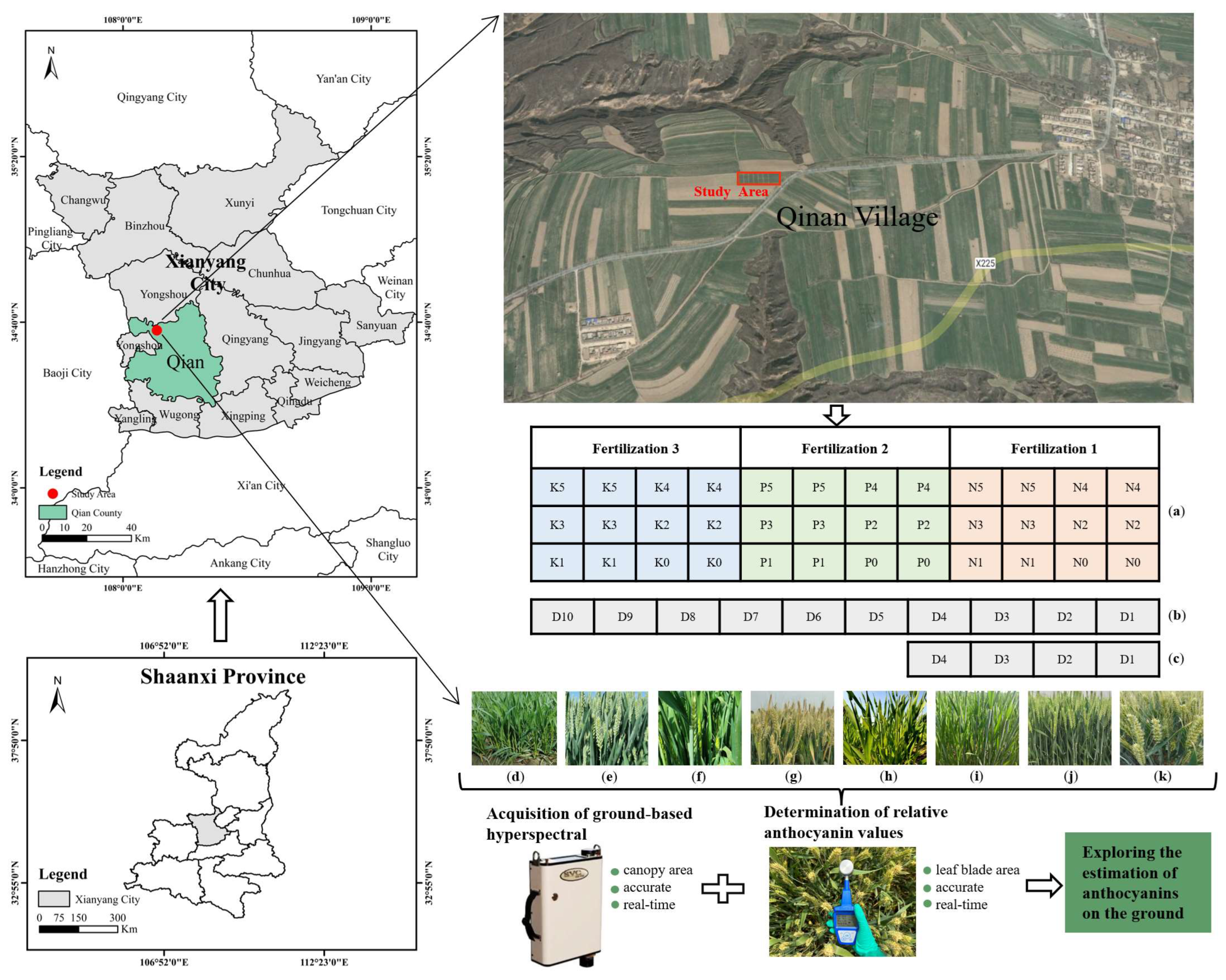
This study was conducted at the test site in Qinan Village, Liangshan Town, Qianxian County, Xianyang City, Shaanxi Province, China (34°38′N, 108°07′E, Figure 1). The study area belongs to the warm-temperate semi-humid continental monsoon climate, characterized by a significant monsoon with rainy summers and dry winters. The area is located in the Loess Plateau gully, with an average elevation of 830 m. The soil type is red-oil soil developed from loess parent material. The crop ripening system is annual, and the main planting structure is a “winter wheat-summer corn” rotation.
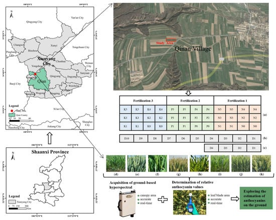
Figure 1.
The schematic of the experimental design. (a) Thirty-six experimental small plots of each experiment; (b) Ten on-farm plots in Experiment I. (c) Four on-farm plots in Experiment II; (d) Booting: 26 March 2017; (e) Heading: 14 April 2017; (f) Flowering: 17 May 2017; (g) Filling: 26 May 2017; (h) Booting: 29 March 2018; (i) Heading: 18 April 2018; (j) Flowering: 7 May 2018; (k) Filling: 22 May 2018. Note: The schematic representation of the satellite in the background (March 2016) was obtained from Google Earth Pro. The letter “D” in table (b) and table (c) represents the on-farm plot.
The winter wheat variety for testing is “Xiao Yan 22”. Winter wheat was cultivated in two experiments, respectively. Experiment I was conducted in 2016–2017 and Experiment II was conducted in 2017-2018. All winter wheat for the experiments was planted on October 2nd. Thirty-six experimental small plots, each 10 m long and 9 m wide, were set up for each experiment. Ten on-farm plots were set up in Experiment I, while four on-farm plots were set up in Experiment II. Nutrients such as nitrogen (N), phosphorus (P) and potassium (K) play an important role in the growth of wheat [37,38,39]. In this study, different levels of single-factor fertilization treatments targeting N, P, and K were set up for the trials to cause differences in winter wheat growth during the same fertility period. The standard N, P, and K fertilizers were individually 90 kg/hm2, 45 kg/hm2, and 60 kg/hm2. The fertilizer applications of small plots are shown in Table 1. Each treatment consisted of one variable fertilizer and two additional standard fertilizers, repeating twice. Besides, all trials of on-farm plots were invariant with the fertilization practices of local farmers. The winter wheat was planted after a one-time application of test fertilizer, and no follow-up fertilizer was applied during the growth period. The field management methods were consistent with local customs.

Table 1.
Fertilizer levels of small plots for the two experiments.
During the growing season, data on canopy reflectance and relative anthocyanin values were collected for each wheat plot under different fertilization treatments, which led to the exploration of terrestrial spectral estimation of anthocyanins.
2.2. Data Acquisition
2.2.1. Hyperspectral Data Acquisition and Preprocessing
The SVC HR-1024i (Spectra Vista Corporation, Poughkeepsie, NY, USA) portable spectrometer was used to measure the spectral reflectance of outdoor winter wheat leaves, adjusting the spectrometer field of view to 25°, with the lens pointing vertically downward almost 1 m from the winter wheat canopy. SVC collected data under clear sky conditions on all dates, and each measurement was taken between 11:00 and 13:00 at the sampling site, as close as possible to a time when the sun’s altitude angle was high to ensure an adequate light source. Moreover, a standard whiteboard correction was performed before determining canopy spectra for an endeavor to ensure that the determined spectra were standardized scientifically. Then, two representative points were chosen in each sample area, where the measurement of canopy spectra was repeated 10 times separately. Finally, the average of the spectra of the two representative points was taken as the spectral reflectance of that sample area. Subsequently, the spectra were processed with Savitzky–Golay smoothing for noise reduction. The operations of the Savitzky–Golay smoothing are done in the Unscrambler X 10.4 software (Camo Software AS, Oslo, Norway), and for all dates and acquisitions, the polynomial order was set as 2, and the number of points on each side was set as five. Besides, the difference method was applied to derive FDS to explore noise reduction further and amplify spectral features.
In the equation, f′(x) is the first-order differential spectra, Rn+1 is the reflectance of the n + 1st raw spectrum, and λn is the position of the nth raw spectrum corresponding to the wavelength in nm.
2.2.2. Determination of Relative Anthocyanin Values
A new multifunctional leaf meter, Dualex Scientific+ (Force-A, Orsay, France), has a measuring area of 5 mm2 and measures the relative values of anthocyanin content by analyzing the shielding effect of anthocyanins on chlorophyll fluorescence. Related studies have shown that relative anthocyanin values measured by Dualex Scientific + correlate with absolute anthocyanin values, suggesting that relative measurements can be used to measure anthocyanin content [40,41]. Besides, the anthocyanin relative values measured by the Dualex Scientific+ were able to observe the growth conditions of wheat at different acquisition dates [42]. In this study, Dualex Scientific+ was used to determine the relative anthocyanin values of winter wheat non-destructively, and the measurement of each sample point immediately followed the SVC measurement. For the measurement, three fresh leaves at each sample point were selected and measured three times from the underneath, middle, to the tip of the leaves to obtain nine anthocyanin values. Finally, the average of the nine anthocyanin values was calculated as the anthocyanin values at the sample site.
2.3. Methods and Models
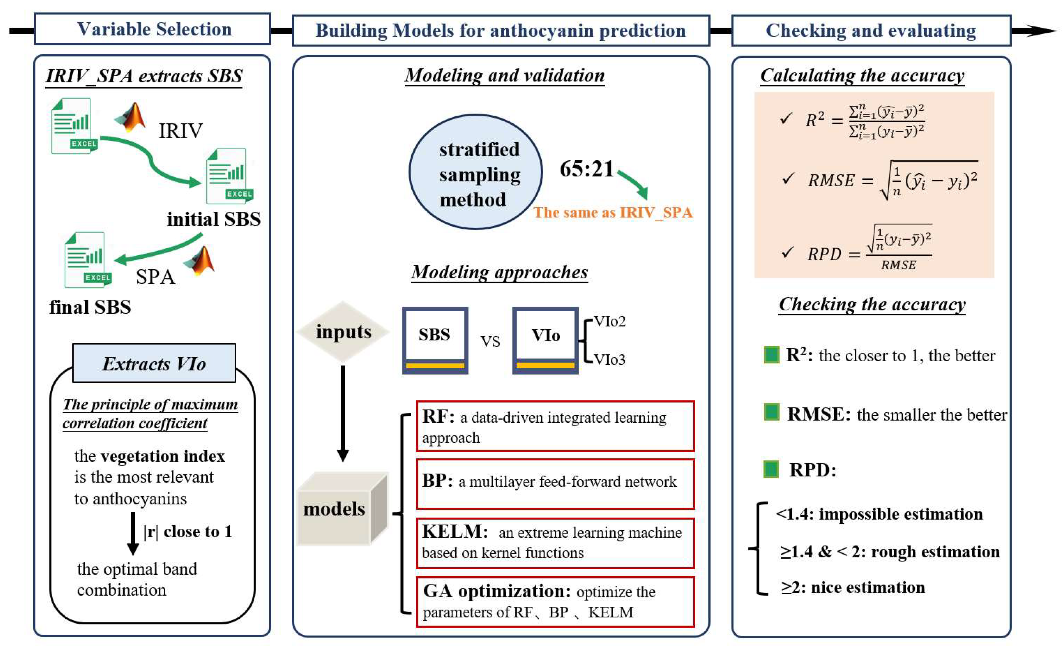
The flowchart of variable selection, model construction and evaluation is shown in the Figure 2. All variable screening methods and modeling approaches were implemented in MATLAB R2022a (Matrix Laboratory, Math-Works, Natick, MA, USA).
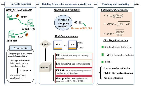
Figure 2.
Flowchart of variable selection, model construction and evaluation.
2.3.1. Variable Selection Method
The iteratively retains informative variables algorithm (IRIV) is a strategy that considers the interactions between variables through random combinations. It classifies variables into four categories: intensely informative, weakly informative, non-informative, and interfering informative, and retains the crucial variables in each iteration by iterating [43]. In this study, the principal components were set to 20 and five cross-validations were performed, thus controlling the search range while validating the models. The successive projections algorithm (SPA) is a forward feature variable selection method. The algorithm utilizes vector projection analysis by projecting wavelengths onto other wavelengths, comparing the magnitude of projected vectors, taking the wavelength with the most significant projected vector as the wavelength to be selected, and then selecting the characteristic wavelengths based on the corrective model and ultimately selecting a combination of variables that contains the tiniest redundant information and the slightest covariance [44]. In this study, the range of selected wavelengths of SPA was set to 1–25, which reduced the search space and improved the computational efficiency of the algorithm.
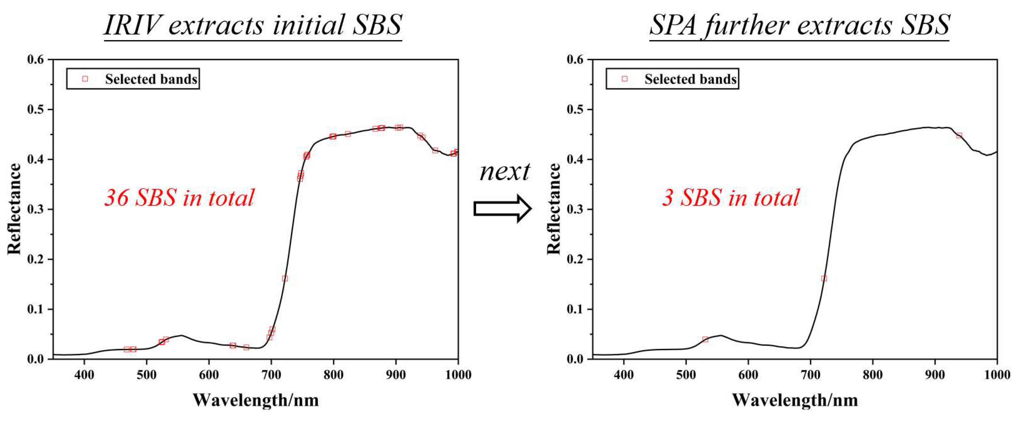
The IRIV operation is fast and good at extracting high-dimensional data [45] but extracts similar wavelength bands [46], whereas SPA can calculate the projection of one wavelength onto other unselected wavelengths in a continuous loop, reducing the covariance between selected wavelengths, avoiding the selection of highly correlated bands, and reducing redundant information [47]; SPA tends to be computationally inefficient [24]. Based on the above realities, the IRIV algorithm and SPA algorithm were used jointly. SPA was utilized to filter the feature bands selected by the IRIV algorithm, which can improve the computational efficiency and extract the influential bands with low multicollinearity. IRIV_SPA combines IRIV and SPA. Specifically, as shown in Figure 3, IRIV first obtains a set of initial SBS associated with winter wheat anthocyanin values, based on which SPA extracts the final SBS.
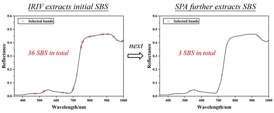
Figure 3.
IRIV_SPA extracts SBS of the original spectrum during the booting stage.
The principle of maximum correlation coefficient, also known as the Pearson correlation coefficient, is a statistical measure of the strength of a linear relationship between two variables. Its core idea is to find the value of correlation between two variables, which ranges from −1 to 1. When the absolute value of the correlation coefficient (|r|) is approximately close to 1, it indicates more correlation, while 0 indicates no linear relationship. This study used the principle of maximum correlation coefficient to select the vegetation index, which is the most relevant to anthocyanins, determining the optimal band combination.
2.3.2. Modeling and Verification
After the results of 85 samples from two experiments were examined and showed no outliers, the results of the data from all stages of winter wheat were further randomly stratified into calibration and validation sets in the ratio of 65:21. The relevant operations were done in MATLAB R2022a. The modeling and verification sets of anthocyanin in winter wheat at each fertility stage had similar statistical characteristics, as shown in Table 2. The maximum value of the validation set was smaller than that of the calibration set, and the minimum value of the validation set was the same as that of the calibration set, implying that the segmentation results were reasonable. The coefficient of variation ranged from 14.51% to 34.60%, showing slight dispersion.

Table 2.
The statistics of anthocyanin values at each fertility stage of winter wheat.
2.3.3. Modeling Approaches
Random forest (RF) is a data-driven integrated learning algorithm based on decision trees [48,49], where each decision tree predicts the inputs, and then the final prediction is derived by voting or averaging. The number of decision trees is called “ntree,” and the number of features divided is called “mtry”. Ntree and mtry are two critical parameters of RF [50]. In this study, ntree was set as 500, and mtry was set by grid search. The related operations are implemented in MATLAB R2022a.
The backward propagation (BP) neural network is a multilayer feed-forward network trained according to the error backpropagation algorithm, which mainly consists of input, hidden, and output layers, each composed of multiple neurons [51]. In a BP neural network, the number of neurons in the input layer is determined by the number of independent variables in the dataset, while the number of neurons in the output layer is decided by the number of target variables [52]. In this study, BP training was implemented by MATLAB R2022a software, and the number of iterations was set to 1000 to train until the loss function tended to flatten and the training curve stabilized, ensuring adequate training.
The kernel extreme learning machine (KELM) is an extreme learning machine (ELM) based on kernel functions. The ELM is a single hidden layer feed-forward neural network. The hidden layer is equivalent to a nonlinear explicit mapping when inputting the weights. After inputting the samples, the samples in the action of this mapping arrive at a linearly divisible space. KELM uses the kernel function to replace the mapping of the hidden node of ELM to map the input data into a high-dimensional space [53], which can better adapt to complex data distributions and deal with nonlinear problems. Compared with traditional neural network algorithms, KELM overcomes the problem of dimensionality catastrophe while avoiding the drawbacks of the instability of ELM, improving generalization performance and nonlinear approximation abilities of conventional models [54]. In this study, the Gaussian kernel function was used to implement KELM, and the relevant operations were implemented in MATLAB R2022a.
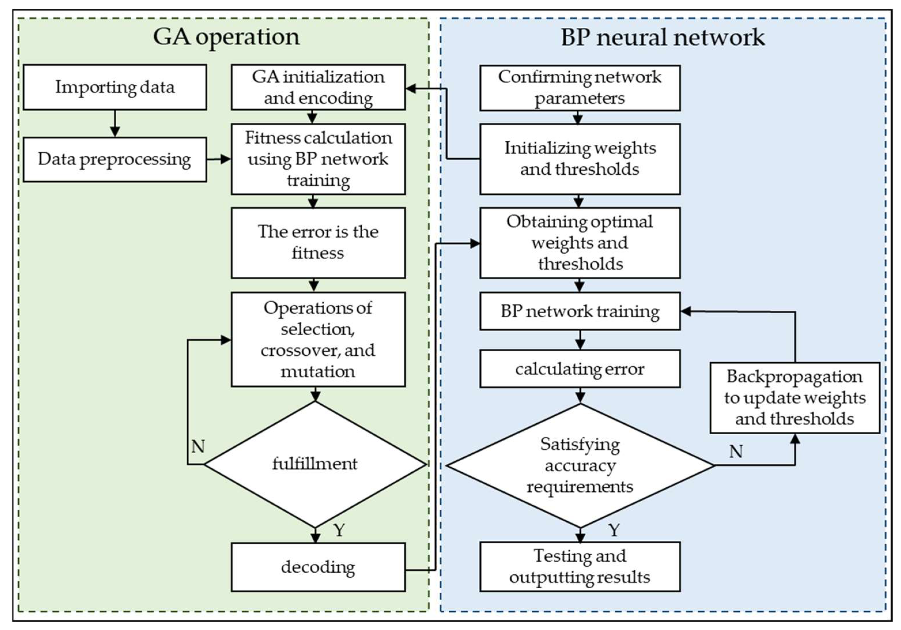
The genetic algorithm (GA) is an optimization algorithm based on biogenetics and evolution [55], which can simulate the basic operations of selection, crossover, and mutation in the evolutionary process to solve complex problems [56]. This study used RF, BP, and KELM models as optimization targets. Then, based on the input data of models, GA parameters were set: the population size is 50, the crossover probability is 0.7, the mutation probability is 0.01, and the maximum number of evolutionary generations is 1000. All the GA operations are implemented in MATLAB R2022a. For instance, the GA-BP calculation process is shown in Figure 4. First, import and preprocess the data. Second, initialize the population and calculate the individual fitness value, select, crossover, and mutate the population, and iterate. Finally, the optimal position is found after satisfying the iteration conditions. Besides, the optimal weights and thresholds are calculated and then substituted into the BP network for training and prediction analysis.
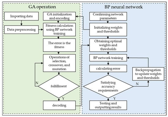
Figure 4.
Algorithm flow of GA_BP network.
2.3.4. Checking the Accuracy of Models
In this study, the coefficient of determination (R2), the root mean square error (RMSE), and the relative prediction deviation (RPD) were selected to test the accuracy of estimation models. The usual range of R2 is [0, 1], and the closer it is to 1 means that models fit better. RMSE is a non-negative value used to measure the deviation between predicted and measured values, and the smaller the value is, the better the model fit. RPD characterizes the robustness of models, and when RPD < 1.4, models cannot predict the sample; when 1.4 ≤ RPD < 2, the sample can be coarsely assessed; when RPD ≥ 2, models are capable of excellent predictive abilities.
3. Results
3.1. Characterizations of Spectrum and Correlation between Anthocyanin and Spectrum
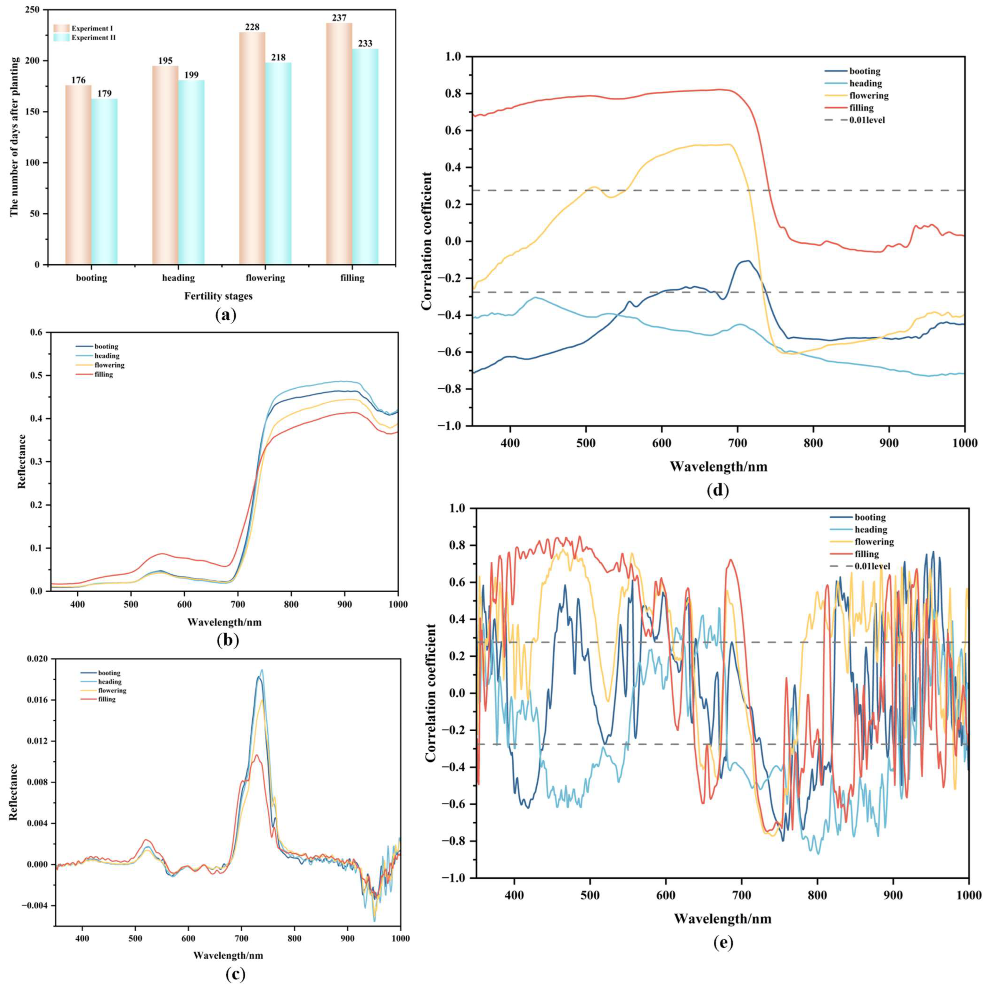
In Figure 5, the spectral characteristics of winter wheat showed a consistent trend across the four fertility stages, and the number of days after sowing for each fertility stage is shown in Figure 5a. As shown in Figure 5b, in the visible range, a reflectance peak was observed near the 550 nm band, and the reflectance increased sharply in the band range of 690–750 nm. In addition, a high reflectance plateau with a reflectance greater than 0.35 is formed in the 760–920 nm range. The correlation coefficients (r) of anthocyanin values and OS of winter wheat are shown in Figure 5d. Anthocyanin values and OS were negatively correlated at the booting and heading stages. Excluding the 600–730 nm range at the booting stage, anthocyanin values and OS at the booting and heading stages were negatively correlated at the 0.01 level, with the highest |r| being 0.71 and 0.73, respectively. During the flowering stage, the anthocyanin values and the OS were significantly and positively correlated in the range of 554–715 nm, with the highest |r| being 0.53, while they were significantly negatively correlated in the range of 735–1000 nm, with the highest |r| being 0.61. During the filling stage, The anthocyanin values were significantly and positively correlated with OS in the 350–740 nm range with the highest |r| of 0.82. According to the order of the number of bands with a correlation level reaching 0.01 significant level from the largest to the smallest, the order of the four fertility stages was heading > booting > flowering > filling, and the correlation between OS and anthocyanin values at heading stage reached 0.01 significant level in all cases.
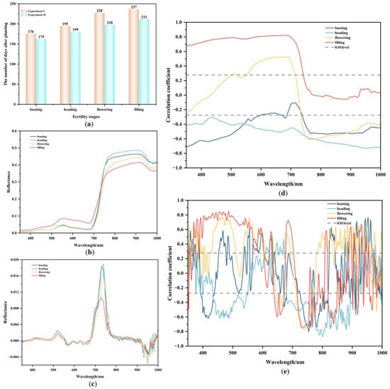
Figure 5.
(a) The number of days after planting. (b) Characterizations of OS at each fertility stage. (c) Characterizations of FDS at each fertility stage. (d) Correlation between anthocyanin and OS; (e) Correlation between anthocyanin and FDS.
As shown in Figure 5c, a conspicuous “red edge” was observed in the 700–750 nm range. The correlation coefficients of FDS and anthocyanin are demonstrated in Figure 5e. The maximum r of FDS and anthocyanin in four stages (booting, heading, flowering, and filing) are located at 754 nm, 801 nm, 464 nm, and 486 nm, where the absolute values of the maximum correlation coefficients were 0.799, 0.870, 0.780, and 0.849, which were higher than that of the stages of OS above.
3.2. Selection of SBS and VIo
3.2.1. Selection of SBS Based on IRIV_SPA
Due to the numerous hyperspectral bands and the extensive computation, reasonable band selection methods should be used to remove redundant information and evade “dimensional catastrophe” in practical applications. In this study, the IRIV-SPA method was used for SBS selection, and as shown in Table 3, the selected bands were mainly located in the red and near-infrared regions, and the near-infrared band was selected in each selection.

Table 3.
Selection of SBS.
3.2.2. Selection of VIo Based on the Principle of Maximum Relevance
Based on the previous experience and knowledge of the characteristic spectral reflectance of winter wheat leaves, ten characteristic parameters closely related to the study of anthocyanin and other phytochromes were selected [57,58]. Firstly, five two-band VIs were calculated, namely, anthocyanin Reflectance Index (ARI), Modified Green Red Vegetation Index (MGRVI), Red Green Ratio Index (R/G), Renormalized Difference Vegetation Index (RDVI) and Optimized Soil-adjusted Vegetation Index (OSAVI). Then, five three-band VIs were calculated, namely, Modified anthocyanin Reflectance Index (MARI), Enhanced Vegetation Index (EVI), Visible-band Reflectance Index (VDVI), Triangular Vegetation Index (TVI), and Plant Senescence Reflectance Index (PSRI). Finally, the VIo2 and VIo3 were further screened out. The formulas and sources of the vegetation indices selected are shown in Table 4.

Table 4.
Vegetation indices.
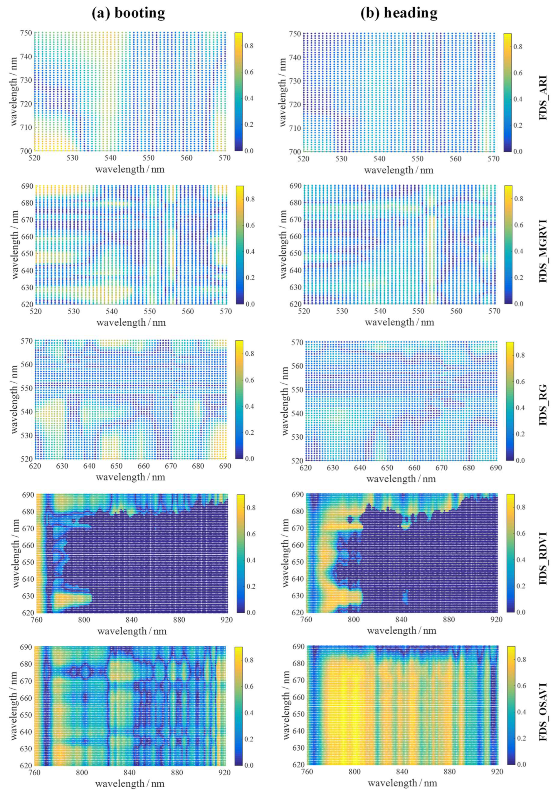
According to the formula of VIs, based on OS and FDS data, the correlation between anthocyanin values and two-band VIs (ARI, MGRVI, RG, RDVI, OSAVI) and three-band VIs (MARI, EVI, VDVI, TVI, PSRI) were calculated for each stage in the hyperspectral range of five bands, namely, blue, green, red, red edge, and near-infrared, respectively. The corresponding correlation heatmaps demonstrated the relationship between the VIs and the anthocyanin values in the two-dimensional and three-dimensional space, whose intensities of color corresponded to the strengths of the correlation. Some of the heat maps are shown in Figure 6 and Figure 7.
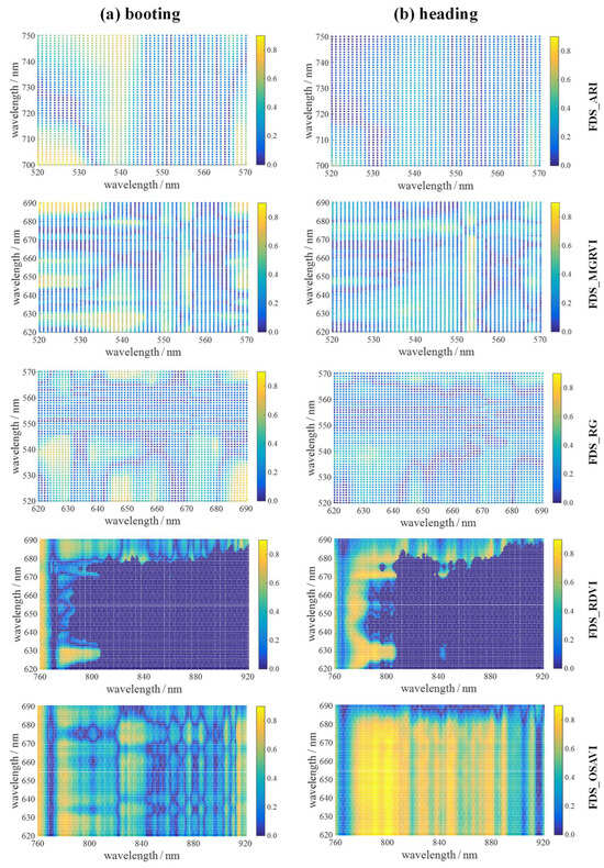
Figure 6.
The heatmaps of |r| of FDS_VIs2 with anthocyanin at the booting stage and heading stage. (a): booting stage; (b): heading stage.
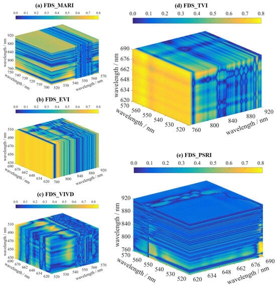
Figure 7.
The heatmaps of |r| of FDS_VIs3 with anthocyanin at the booting stage. (a): FDS_MARI; (b): FDS_EVI; (c): FDS_VIVD; (d): FDS_TVI; (e): FDS_PSRI.
The selected VIo2 and VIo3 are shown in Table 5 and Table 6, and the results showed significant correlations (p < 0.01) between anthocyanin and VIo2 and VIo3. In addition, the |r| of OS_VIo2 with anthocyanins was 0.41–0.85. The |r| of OS_VIo3 with anthocyanins was 0.40–0.83. The |r| of FDS_VIo2 with anthocyanins was 0.55–0.89. The |r| of FDS_VIo3 with anthocyanins was 0.70–0.89. Overall, FDS optimized the correlation between VIo and anthocyanin values, and FDS_VIo band combinations differ significantly from those of OS_VIo bands, mainly because FDS reduces overlap and autocorrelation between spectral bands, expanding the discrepancies between spectra [64].

Table 5.
|r| between VIo2 and anthocyanin at each fertility stage.

Table 6.
|r| between VIo3 and anthocyanin at each fertility stage.
3.3. Anthocyanin Estimation Based on Models and GA Optimization
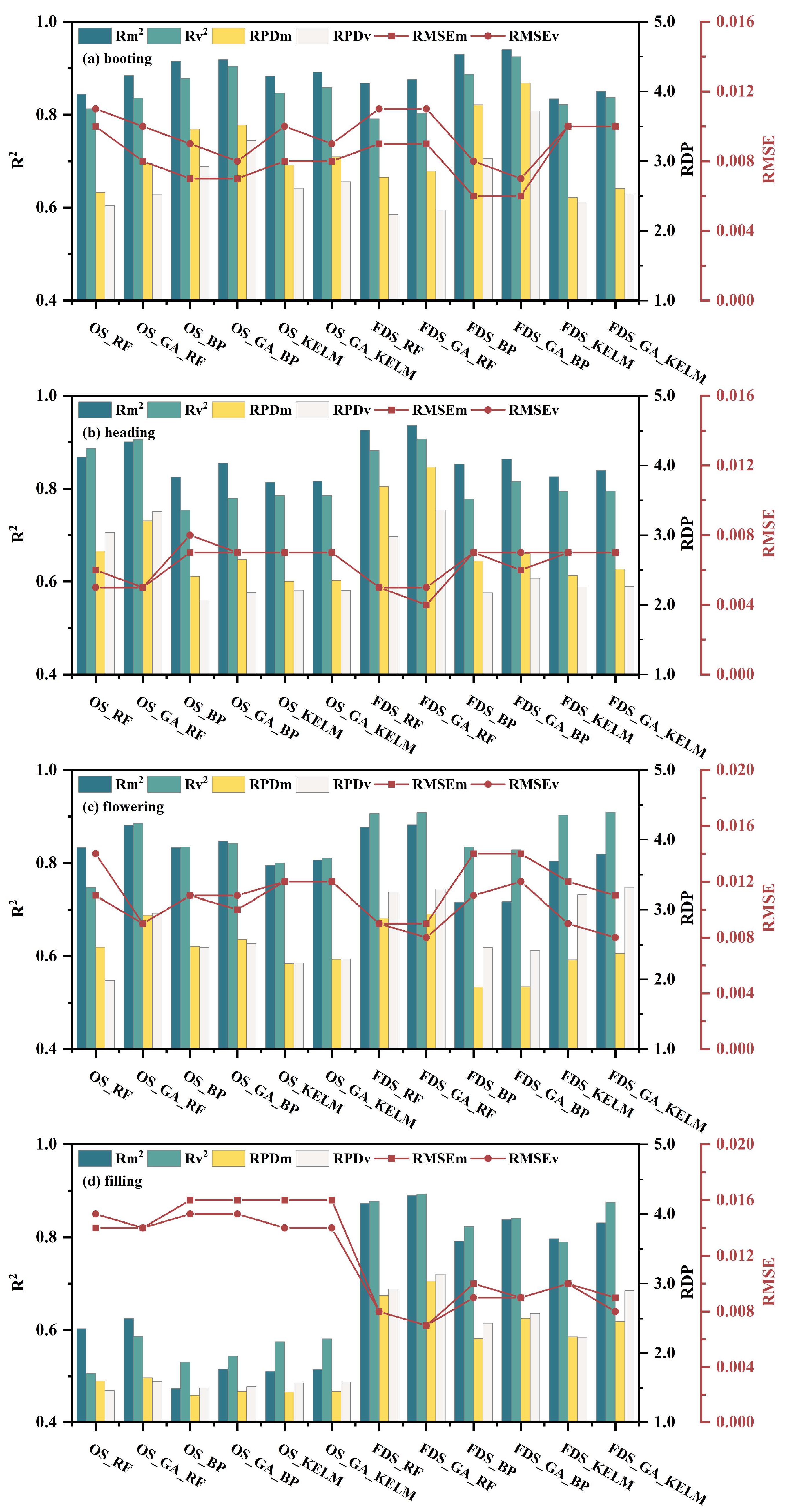
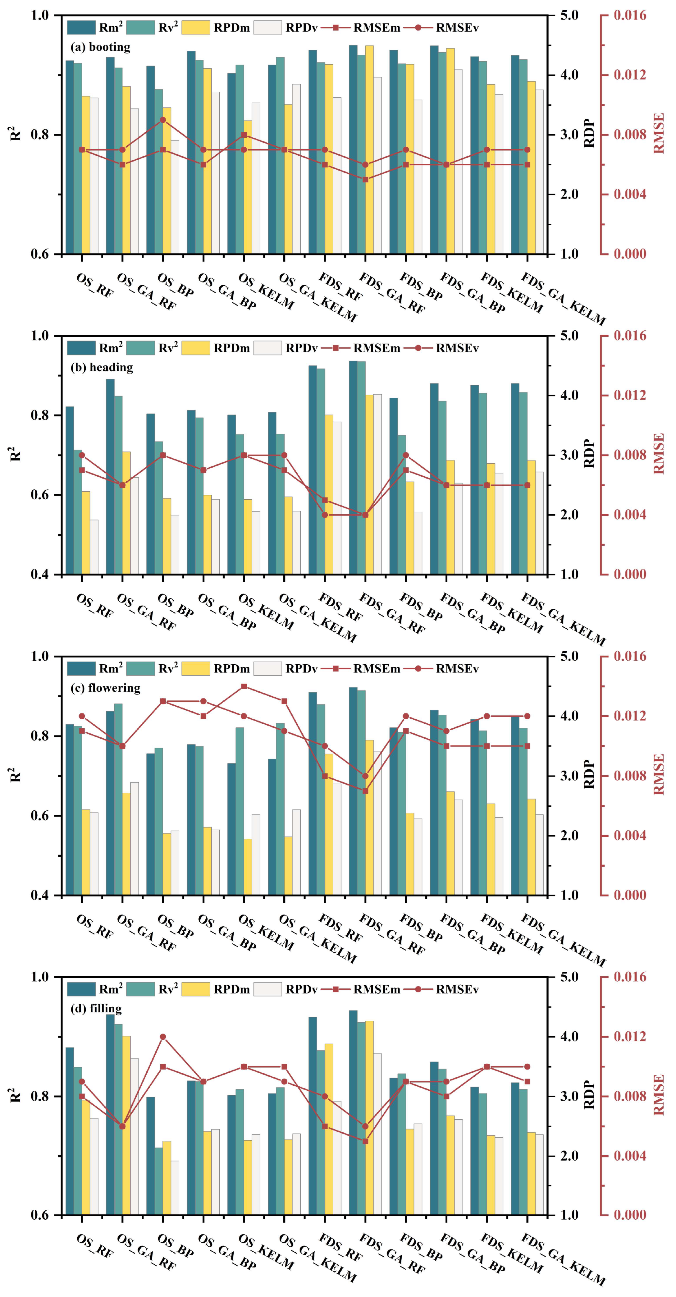
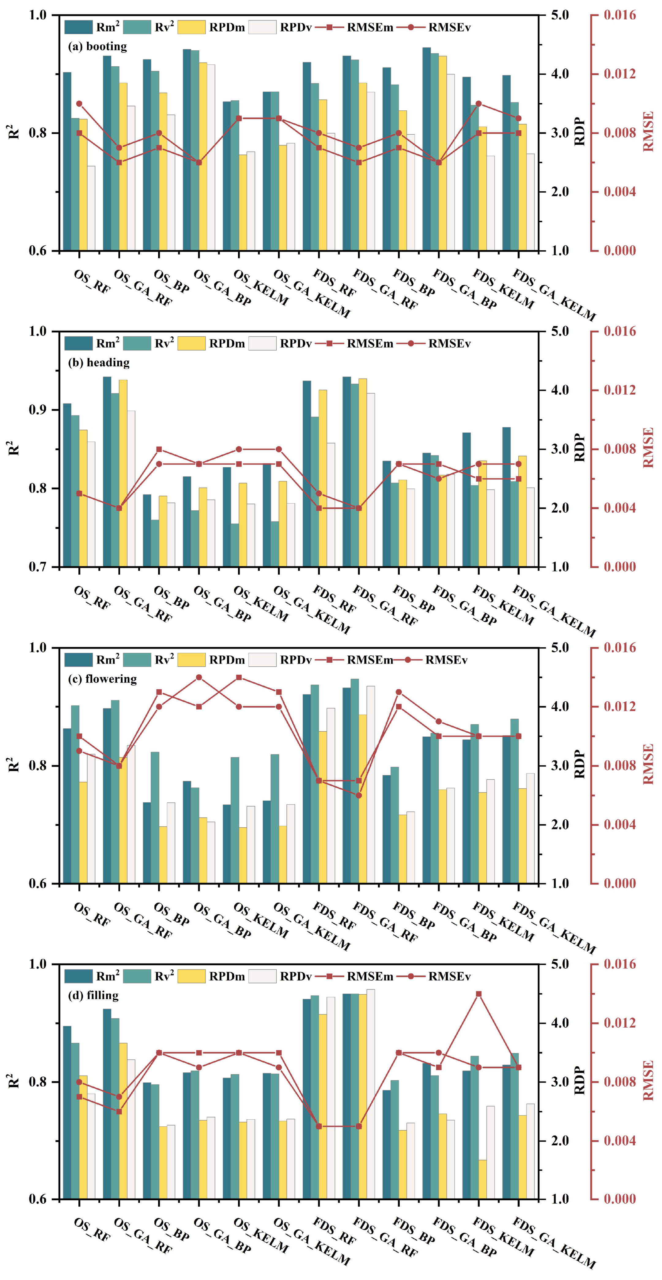
In this study, the format “Processing_Model (Parameter)” is used to display a specific model, and the format “MLs (Parameter)” is used to represent all models of that parameter type. The model performances of MLs (SBS), MLs (VIo2), and MLs (VIo3) are shown in Figure 8, Figure 9 and Figure 10, respectively. Namely, the models with SBS as input variables are shown in Figure 8, and those with VIo2 and VIo3 as input variables are shown in Figure 9 and Figure 10 separately. “m” stands for modeling set, and “v” stands for validation set. R2 is the general name of Rm2 and Rv2, RPD is the general name of RPDm and RPDv, and RMSE is the general name of RMSEm and RMSEv.
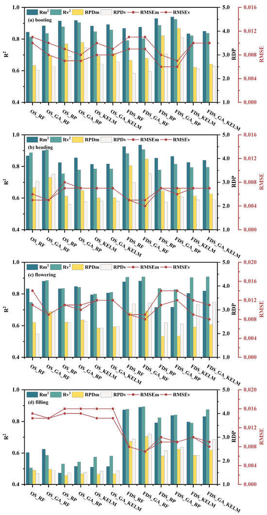
Figure 8.
The accuracy parameters of MLs (SBS) for each fertility stage. (a): booting stage; (b): heading stage; (c): flowering stage; (d): filling stage. Rm2 represents R2 of the modeling set, Rv2 represents R2 of the verification set, RPDm represents RPD of the modeling set, RPDv represents RPD of the verification set, RMSEm represents RMSE of the modeling set, and RMSEv represents RMSE of the verification set.

Figure 9.
The accuracy parameters of MLs (VIo2) for each fertility stage. (a): booting stage; (b): heading stage; (c): flowering stage; (d): filling stage. Rm2 represents R2 of the modeling set, Rv2 represents R2 of the verification set, RPDm represents RPD of the modeling set, RPDv represents RPD of the verification set, RMSEm represents RMSE of the modeling set, and RMSEv represents RMSE of the verification set.

Figure 10.
The accuracy parameters of MLs (VIo3) for each fertility stage. (a): booting stage; (b): heading stage; (c): flowering stage; (d): filling stage. Rm2 represents R2 of the modeling set, Rv2 represents R2 of the verification set, RPDm represents RPD of the modeling set, RPDv represents RPD of the verification set, RMSEm represents RMSE of the modeling set, and RMSEv represents RMSE of the verification set.
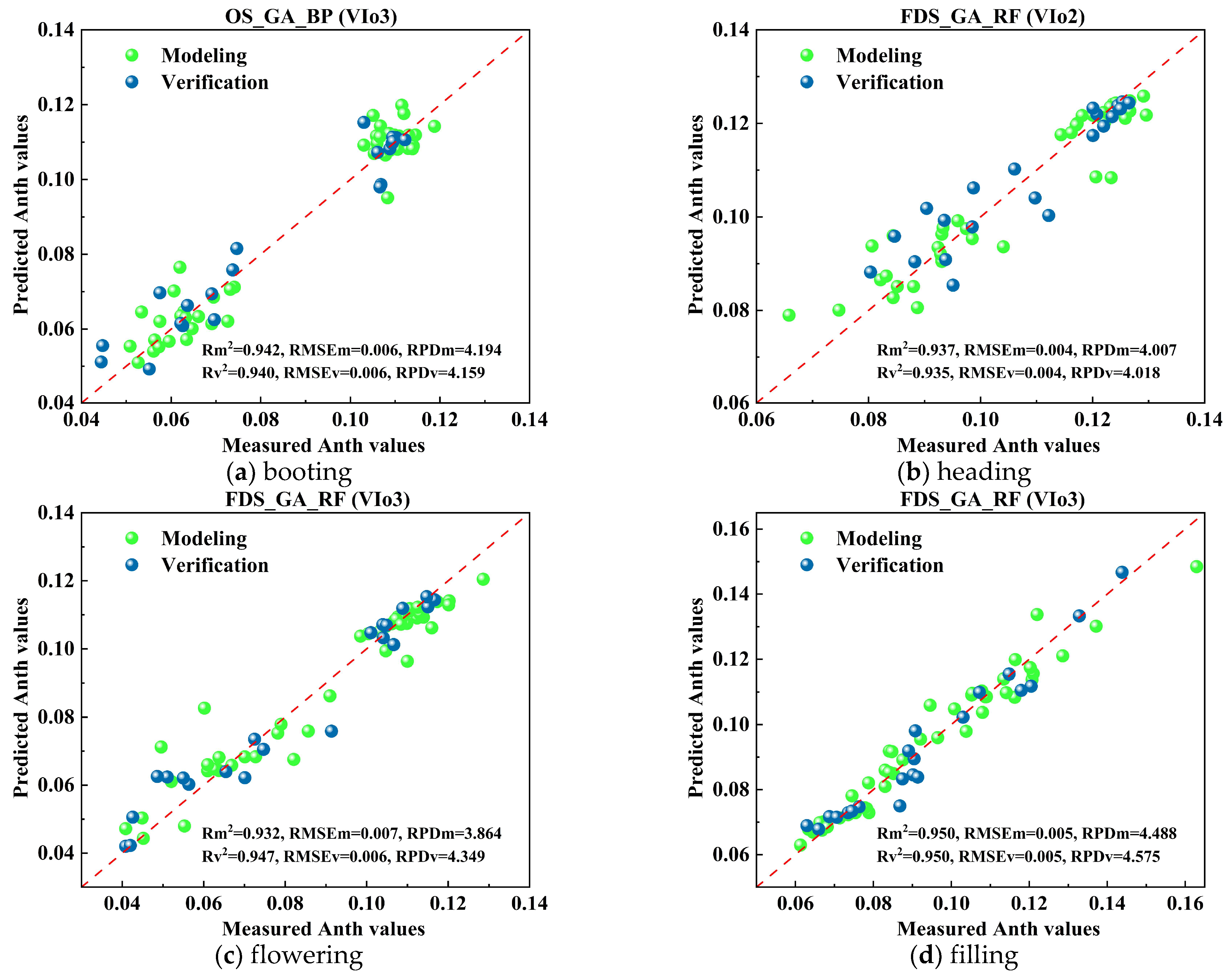
In the booting stage, OS_GA_BP (VIo3) worked best with Rm2 = 0.942, RPDm = 4.194, Rv2 = 0.940, and RPDv = 4.159. In the heading stage, FDS_GA_RF (VIo2) demonstrated prime performance, resulting in Rm2 = 0.937, RPDm = 4.007, Rv2 = 0.935, and RPDv = 4.018. In the flowering stage, FDS_GA_RF (VIo3) achieved the highest accuracy, with Rm2 = 0.932, RPDm = 3.864, Rv2 = 0.947, and RPDv = 4.349. In the booting stage, FDS_GA_RF (VIo3) performed best, with Rm2 = 0.950, RPDm = 4.488, Rv2 = 0.950, and RPDv = 4.575.
The favorable effects of the first-order spectral transformation can likewise be seen in the model performances. For MLs (SBS), during the booting, heading, and flowering stages, compared with the best OS_MLs (SBS), the Rm2 of the best FDS_MLs (SBS) was improved by 2.40%, 3.88%, and 0.11%, and the Rv2 was enhanced by 2.32%, 0.11%, and 2.60%, respectively. During the filling stage, the modeling effects were poor, as the RPD of each OS_ML was less than 2.0. Besides, compared to the corresponding OS_MLs, the Rm2 of FDS_RF, FDS_GA_RF, FDS_BP, FDS_GA_BP, FDS_KELM, and FDS_GA_KELM are respectively improved by 44.78%, 42.40%, 67.44%, 62.40%, 55.97%, and 61.36%, whereas the Rv2 was enhanced by 73.32%, 52.39%, 54.99%, 54.60%, 37.39% and 50.60%. For MLs (VIo2), during the four stages, compared to the best OS_MLs (VIo2), the best FDS_MLs (VIo2) improved the Rm2 by 0.75–6.96% and the Rv2 by 0.33–10.26%. For MLs (VIo3), in all four stages, compared to the best OS_MLs (VIo3), the Rm2 of the best FDS_MLs (VIo3) enhanced by 0–3.90%, although the Rv2 decreased by 0.53% at the booting period, it improved by 1.30–4.63% in the remaining three stages. Moreover, in all the models, the Rv2 values of the optimal models of FDS were all greater than 0.89. In summary, the optimal FDS_MLs were overall better than the optimal OS_MLs in all stages, indicating that the first-order differential transformation could improve the inversion effects of SBS and VIo on anthocyanin.
In the MLs (VIo) of all the stages, the R2 of the GA_RF (VIo) exceeded 0.84, and the RPD outweighed 2.62. In the booting stage, the R2 of GA_RF (VIo) reached 0.91, the RPD attained 3.43, and GA_RF (VIo) had the optimal inversion values in the heading, flowering, and filling stages. In the MLs (SBS) of all the stages, GA_RF (SBS) was also the best model in each stage of heading, flowering, and filling, and in the booting stage, GA_RF (SBS) had a brilliant fit with Rv2 = 0.836 and RPDv = 2.518. Therefore, GA_RF performed steadily in the four stages compared to the other models.
Compared to the use of RF, BP, and KELM exclusively, the joining of GA optimization improved the R2 of the MLs (SBS) by 0.00%-18.47% (except for FDS_GA_BP (SBS) at flowering stage), improved the R2 of the MLs (VIo2) by 0.13–18.93% (except for FDS_GA_RF (VIo2) at booting stage), and improved the R2 of the MLs (VIo3) by 0.12%-10.67% (except for FDS_GA_BP (SBS) at flowering stage).
The optimal model for each stage of winter wheat is shown in Figure 11. In each stage of winter wheat, VIo was the best model parameter. The optimal MLs (VIo) improved the estimation R2 of anthocyanin by 0.11–6.74% compared with the optimal MLs (SBS), which indicated that VIo was more suitable than SBS for estimating anthocyanin values of winter wheat in this study. In addition, VIo3, besides being the optimal model parameter for the three stages of booting, flowering, and filling, also had a high estimation effect in FDS_GA_RF(VIo3) at the heading stage, with Rv2 = 0.933 and RPDv = 3.949. Therefore, VIo3 is generally well-suited for the estimation of anthocyanins.
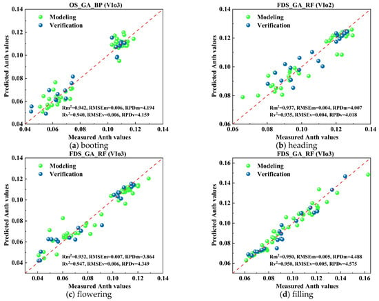
Figure 11.
Optimal predicted anthocyanin values and measured values for each fertility stage. (a): booting stage; (b): heading stage; (c): flowering stage; (d): filling stage.
4. Discussion
As shown in Table 7, all the discussion items are mainly divided into three points, which are developed from the band selection, the influencing factors of model accuracy, and GA optimization, respectively.

Table 7.
Discussion items of the study.
4.1. BSM: Screening for Optimal Sensitive Bands and Band Combinations
This study estimated winter wheat anthocyanins using the characteristic bands extracted by IRIV_SPA. OS_ML during the filling stage(0.473 < R2 <0.625, 1.4 < RPD < 2.0) could only roughly estimate anthocyanins with poor results. Except for the OS_ML in the filling period, the rest of the models were modeled better, with Rm2 ranging from 0.716 to 0.940, RPDm ranging from 1.890 to 4.122, Rv2 ranging from 0.747 to 0.925, and RPDv ranging from 1.985 to 3.718. It is seen from the results of the modeling and validation that extracting SBS by IRIV_SPA is of some feasibility for estimating the anthocyanins of winter wheat. The results showed that the bands screened in all stages of winter wheat were mainly concentrated at 720–1000 nm, which is in the red and near-infrared regions. The near-infrared band would be selected in the SBS of each selection process, which indirectly indicates that certain near-infrared bands have some sensitivity to the anthocyanin values of winter wheat. It is generally recognized that the near-infrared band is mainly affected by essential components of the leaf, such as proteins and leaf water [65]. However, the protein and water content in leaves can indirectly affect the anthocyanin content. For instance, anthocyanins can be protected from direct light damage by binding proteins in a covalent and non-covalent manner within the leaf [66,67]. Besides, anthocyanin molecules may form non-covalent interactions, such as hydrogen bonds with water molecules in the leaf, which stabilize the anthocyanin state [68]. Cheng et al. [69] showed that the protein and water content in winter wheat leaves can indirectly affect the chlorophyll content. Curran et al. [70] also showed similar results in a spectroscopic study of biochemical components of plant leaves. Therefore, there is a high probability that bands in the near-infrared will be found to have a contribution to the estimation of anthocyanin.
Traditional VIs utilize only specified band combinations, which can be limited in their usefulness in different situations. Previous studies have found that seeking VIo can play a terrific role in VIs and improve prediction [71,72]. To illustrate, Tuya et al. [73] selected the optimal bands for NDVI, RVI, and three-band chlorophyll content index, and the results showed that the optimized VIs were more accurate in predicting the total nitrogen yield of maize than the original VIs. In this study, the correlation analysis matrix between VIs and anthocyanin under OS and FDS data was established to exhaustively find the 10 VIo combined by the best band combinations according to the principle of maximum correlation coefficient. The band combinations of VIo showed that different band combinations were selected for the same vegetation index in OS and FDS data, possibly caused by the different spectral characteristics and information reflected by OS and FDS [74]. The FDS transformation can limit the noisy backgrounds, such as soil, to a certain extent [75], and the optimal band combinations of OS may pay attention to the sensitivities of some specific bands to the anthocyanin value. In comparison, the optimal band combinations of FDS may attach more importance to the trends of the spectral curves [27]. Additionally, the band combinations selected for the same vegetation index were not identical for different wheat growth stages, mainly associated with different sensitivities that anthocyanin values generated to spectra at various stages of winter wheat. Furthermore, the consequences of band combinations of MGRVI, RG, RDVI, and OSAVI showed that the bands selected for VIs in the same band range were divergent. The potential reason for this may be that diverse VIs combine bands through distinct formulas, which have dissimilar spectral information [76] and distinguishable roles in characterizing the anthocyanin values of winter wheat.
All in all, screening SBS and VIo as model input variables could effectively estimate anthocyanin values. Besides, compared with SBS, VIo, as a parameter of the best model in each stage, was more suitable for estimating anthocyanin values, and this result is homologous to that of a study by Jiang et al. [14]. The possible reason for the above result is that these VIo consist of a combination of bands in each spectral range (blue, green, red, red edge, NIR), which can provide more spectral information compared to SBS and eliminate the influence of atmosphere and soil to a certain extent [77]. The methodologies of band screening adopted in this study can provide references for monitoring studies of other related biochemical parameters.
4.2. Predictive Accuracy of Anthocyanin and Its Influencing Factors
It has been shown that there is a difference in band information after spectral transformations, which amplifies the available information in the data [78,79,80]. Our study found that among the MLs(SBS) and MLs(VIo), The GA_RF model behaved both stably and marvelously in the four stages, probably because of the intense noise immunity and generalization ability of the model built by the GA_RF, which can solve many covariance problems of the unbalanced dataset and reduce data errors [81]. Although the OS_GA_BP(VIo2) model had the best modeling among all the models at the booting stage, the Rv2 of OS_GA_KELM(VIo2) was 0.05 higher than that of OS_GA_BP(VIo2) in ML(VIo2), and as far as the fitting effect was concerned, it was OS_GA_KELM (VIo2) that did the best. Therefore, it is essential to calibrate and evaluate competitive estimation models based on specific experimental datasets. Alternatively, under the FDS transformation, the R2 of the FDS_GA_BP (SBS) model improved by more than 1% compared with OS_GA_BP (SBS) at the booting, heading, and filling stages, except at the flowering stage. Also, except for the booting stage, the R2 of the FDS_GA_RF (SBS) model improved by more than 0.1% compared with OS_GA_RF (SBS). Withal, The R2 of FDS_RF (VIo2), FDS_GA_RF (VIo2), FDS_BP (VIo2), and FDS_GA_BP (VIo2) all improved by more than 0.1% compared to the corresponding OS_ML in all stages of the winter wheat, yet there were no consistent findings for FDS_KELM (VIo2), and FDS_GA_KELM (VIo2). Furthermore, the model accuracy of FDS_GA_RF (VIo3) was higher than that of OS_GA_RF (VIo3) in all stages, while the remaining models had no consistent conclusions. The above models, which have no consistent findings, may be unable to present regular effects due to the role of data collection stages [82], data characteristics and quality [83], and model parameter configurations [84]. No transformation approach or ML appears to apply to all conditions [85]. Thus, it is crucial to compare transformation treatments and multiple methods based on different periods of data and input variables.
Our study further showed that FDS affected the modeling accuracy to varying degrees. Among them, during the prediction process with SBS as the parameter, the variation of R2 of FDS_ML(SBS) compared with OS_ML(SBS) at the booting, heading, and flowering stages was within ±16%, whereas the R2 of FDS_ML(SBS) improved by more than 44% compared with that of OS_ML(SBS) at the filling stage, which might be attributed to the possibility that the slope of the absorption peaks of anthocyanins during the filling stage varied more from the OS, resulting in an enormous variation of FDS [86], providing more valuable information for modeling.
4.3. Optimizing RF, BP, and KELM with GA
GA is a stochastic global search and optimization method developed by emulating selection mechanisms and genetic variation in nature [87]. GA can optimize the parameters of RF, such as the number of decision trees and the tree depth [88], and others. GA can also optimize the parameters of BP and KELM, like searching for superior weights and bias value combinations [53,89].
It has been shown that the use of GA can improve the accuracy of the modeling. For example, Atefeh et al. [90] applied GA to calculate the optimal hyperparameters of RF, which showed a general improvement in the prediction performance of GA_RF compared to RF. Shi et al. [91] used GA to perform parameter optimization of the BP model estimating the chlorophyll content of winter wheat, in which the modeling accuracy of GA_BP was higher than that of the BP model. Zheng et al. [92] used the GA to optimize ELM for shallow sea bathymetry inversion, confirming that the accuracy of the GA_ELM model was higher than that of the ordinary ELM model. Our study also found that the simulation accuracy of the models optimized by GA was generally higher. Compared to using RF, BP, and KELM exclusively, the joining of GA optimization improved the R2 by 0.00%-18.93% over the original models (Excluding FDS_GA_BP (SBS) at the flowering stage, OS_GA_RF (VIo2) at the booting stage, and OS_GA_BP (VIo3) at the flowering stage). Synthesizing, GA can effectively emphasize the effects of distinct models, probably seeing that GA can perform an exhaustively optimal search in the parameter space and introduce new gene combinations through crossover and mutation operations, thus increasing the diversity and exploration abilities of the model, contributing to the fabulous adaptation of the model to various datasets and problems, as well as enforcing its generalization ability and prediction accuracy [93].
5. Conclusions
In this study, the anthocyanin content of winter wheat at different growth stages was estimated based on OS and FDS data of ground-based hyperspectral (SVC), using SBS, VIo2 and VIo3 as inputs and combining with modeling methods such as RF, BP, KELM, and GA optimization models. The main conclusions are as follows:
- (1)
- Among the models, the GA_RF model was consistently excellent, and VIo3 was remarkable for estimating anthocyanin values. The model GA_RF of FDS data based on VIo3 during the filling stage had the best performance (Rv2 = 0.950, RMSEv = 0.005, RPDv = 4.575) among all the models.
- (2)
- The first-order differential processing can effectively improve the correlation between anthocyanin and SBS, VIo2, and VIo3. The model performances of the FDS were better than that of OS on the whole, and the Rv2 values of the optimal models of FDS were all greater than 0.89.
- (3)
- The GA-optimized models showed an overall increase of 0.00% to 18.93% in the explanation of anthocyanins.
Author Contributions
Conceptualization, H.M. and X.C.; methodology, H.M.; software, H.M.; validation, H.M., X.C. and Q.C.; formal analysis, H.M., X.C. and Y.G.; investigation, H.M., Q.W. and R.Z.; resources, Q.C.; data curation, H.M.; writing—original draft preparation, H.M.; writing—review and editing, H.M.; visualization, H.M.; supervision, Y.G.; project administration, Q.C.; funding acquisition, Q.C. All authors have read and agreed to the published version of the manuscript.
Funding
This research was funded by the National Natural Science Foundation of China (41701398).
Data Availability Statement
The original contributions presented in the study are included in the article, further inquiries can be directed to the corresponding author.
Acknowledgments
We sincerely appreciate the assistance and support of the teachers and all the students in the lab. Moreover, we treasure all the constructive observations and recommendations the editors and anonymous reviewers provided.
Conflicts of Interest
The authors declare no conflicts of interest.
References
- Xie, L.; Lu, Y.; Zhou, Y.; Hao, X.; Chen, W. Functional Analysis of a Methyltransferase Involved in Anthocyanin Biosynthesis from Blueberries (Vaccinium corymbosum). J. Agric. Food Chem. 2022, 70, 16253–16262. [Google Scholar] [CrossRef] [PubMed]
- Ceferino, C.; María José, A.-G.; Monika, V.; Marta, F.-G.; Gerardo, F.B. A Novel Ultrasound-Assisted Extraction Method for the Analysis of Anthocyanins in Potatoes (Solanum tuberosum L.). Antioxidants 2021, 10, 1375. [Google Scholar] [CrossRef] [PubMed]
- Averina, N.; Savina, S.; Dremuk, I.; Yemelyanava, H.; Pryshchepchyk, Y.; Usatov, A. Influence of 5-aminolevulinic acid on physiological and biochemical characteristics of winter wheat varieties with different levels of anthocyanins in coleoptiles. Proc. Natl. Acad. Sci. Belarus Biol. Ser. 2022, 67, 135–146. [Google Scholar] [CrossRef]
- Bhatt, V.; Sendri, N.; Swati, K.; Devidas, S.; Bhandari, P. Identification and quantification of anthocyanins, flavonoids and phenolic acids in flowers of Rhododendron arboreum and evaluation of their antioxidant potential. J. Sep. Sci. 2022, 45, 2555–2565. [Google Scholar] [CrossRef] [PubMed]
- Chandra Singh, M.; Price, W.; Kelso, C.; Arcot, J.; Probst, Y. Measuring the anthocyanin content of the Australian fruit and vegetables for the development of a food composition database. J. Food Compos. Anal. 2022, 112, 104697. [Google Scholar] [CrossRef]
- Nitasaka, E.; Hoshino, A. Anthocyanin mutants of Japanese and common morning glories exhibit normal proanthocyanidin accumulation in seed coats. Plant Biotechnol. 2018, 35, 259–266. [Google Scholar] [CrossRef]
- Gitelson, A.; Keydan, G.; Merzlyak, M.; Gitelson, C. Three-Band Model for Noninvasive Estimation of Chlorophyll Carotenoids and Anthocyanin Contents in Higher Plant Leaves. Geophys. Res. Lett. 2006, 33, L11402. [Google Scholar] [CrossRef]
- Yang, X.; Zhang, J.; Guo, D.; Xiong, X.; Chang, L.; Niu, Q.; Huang, D. Measuring and evaluating anthocyanin in lettuce leaf based on color information. IFAC-PapersOnLine 2016, 49, 96–99. [Google Scholar] [CrossRef]
- Duan, D.; Zhao, C.; Li, Z.; Yang, G.; Yang, W. Estimating total leaf nitrogen concentration in winter wheat by canopy hyperspectral data and nitrogen vertical distribution. J. Integr. Agric. 2019, 18, 1562–1570. [Google Scholar] [CrossRef]
- Yin, Q.; Zhang, Y.; Li, W.; Wang, J.; Wang, W.; Ahmad, I.; Zhou, G.; Huo, Z. Estimation of Winter Wheat SPAD Values Based on UAV Multispectral Remote Sensing. Remote Sens. 2023, 15, 3595. [Google Scholar] [CrossRef]
- Zhu, Z.; Li, T.; Cui, J.; Shi, X.; Chen, J.; Wang, H. Non-destructive estimation of winter wheat leaf moisture content using near-ground hyperspectral imaging technology. Acta Agric. Scand. Sect. B-Soil Plant Sci. 2020, 70, 294–306. [Google Scholar] [CrossRef]
- Yang, C.; Xu, J.; Feng, M.; Bai, J.; Sun, H.; Song, L.; Wang, C.; Yang, W.; Xiao, L.; Zhang, M.; et al. Evaluation of Hyperspectral Monitoring Model for Aboveground Dry Biomass of Winter Wheat by Using Multiple Factors. Agronomy 2023, 13, 983. [Google Scholar] [CrossRef]
- Luo, L.; Chang, Q.; Gao, Y.; Jiang, D.; Li, F. Combining Different Transformations of Ground Hyperspectral Data with Unmanned Aerial Vehicle (UAV) Images for Anthocyanin Estimation in Tree Peony Leaves. Remote Sens. 2022, 14, 2271. [Google Scholar] [CrossRef]
- Jiang, S.; Chang, Q.; Wang, X.; Zheng, Z.; Zhang, Y.; Wang, Q. Estimation of Anthocyanins in Whole-Fertility Maize Leaves Based on Ground-Based Hyperspectral Measurements. Remote Sens. 2023, 15, 2571. [Google Scholar] [CrossRef]
- Gutiérrez, S.; Tardaguila, J.; Fernández-Novales, J.; Diago, M.-P. On-the-go hyperspectral imaging for the in-field estimation of grape berry soluble solids and anthocyanin concentration: Hyperspectral imaging for in-field grape estimation. Aust. J. Grape Wine Res. 2018, 25, 127–133. [Google Scholar] [CrossRef]
- Liu, H.; Zhu, H. Hyperspectral characteristic analysis for leaf nitrogen content in different growth stages of winter wheat. Appl. Opt. 2016, 55, D151. [Google Scholar] [CrossRef]
- Liu, H.; Zhu, H.; Wang, P. Quantitative modelling for leaf nitrogen content of winter wheat using UAV-based hyperspectral data. Int. J. Remote Sens. 2016, 38, 2117–2134. [Google Scholar] [CrossRef]
- Zhu, H.; Liu, H.; Xu, Y.; Guijun, Y. UAV-based hyperspectral analysis and spectral indices constructing for quantitatively monitoring leaf nitrogen content of winter wheat. Appl. Opt. 2018, 57, 7722. [Google Scholar] [CrossRef]
- Chen, X.; Lv, X.; Ma, L.; Chen, A.; Zhang, Q.; Zhang, Z. Optimization and Validation of Hyperspectral Estimation Capability of Cotton Leaf Nitrogen Based on SPA and RF. Remote Sens. 2022, 14, 5201. [Google Scholar] [CrossRef]
- Shu, M.; Zhu, J.; Yang, X.; Gu, X.; Li, B.; Ma, Y. A spectral decomposition method for estimating the leaf nitrogen status of maize by UAV-based hyperspectral imaging. Comput. Electron. Agric. 2023, 212, 108100. [Google Scholar] [CrossRef]
- Hu, Y.; Kang, Z. The Rapid Non-Destructive Detection of Adulteration and Its Degree of Tieguanyin by Fluorescence Hyperspectral Technology. Molecules 2022, 27, 1196. [Google Scholar] [CrossRef] [PubMed]
- Liu, Y.; Wang, T.; Su, R.; Hu, C.; Chen, F.; Cheng, J. Quantitative Evaluation of Color, Firmness, and Soluble Solid Content of Korla Fragrant Pears via IRIV and LS-SVM. Agriculture 2021, 11, 731. [Google Scholar] [CrossRef]
- Zhang, L.; Nie, P.; Zhang, S.; Zhang, L.; Sun, T. Research on Defect Detection in Kubo Peach Based on Hyperspectral Imaging Technology Combined with CARS-MIV-GA-SVM Method. Foods 2023, 12, 3593. [Google Scholar] [CrossRef] [PubMed]
- Sudu, B.; Rong, G.; Guga, S.; Li, K.; Zhi, F.; Guo, Y.; Zhang, J.; Bao, Y. Retrieving SPAD Values of Summer Maize Using UAV Hyperspectral Data Based on Multiple Machine Learning Algorithm. Remote Sens. 2022, 14, 5407. [Google Scholar] [CrossRef]
- Liang, K.; Liu, Q.; Pan, L.; Chen, M. Detection of soluble solids content in ‘Korla fragrant pear’ based on hyperspectral imaging and CARS-IRIV algorithm. J. Nanjing Agric. Univ. 2018, 41, 760–766. [Google Scholar]
- Zhang, J.; Cheng, T.; Guo, W.; Xu, X.; Qiao, H.; Xie, Y.; Ma, X. Leaf area index estimation model for UAV image hyperspectral data based on wavelength variable selection and machine learning methods. Plant Methods 2021, 17, 49. [Google Scholar] [CrossRef] [PubMed]
- Fang, H.; Man, W.; Liu, M.; Zhang, Y.; Chen, X.; Li, X.; He, J.; Tian, D. Leaf Area Index Inversion of Spartina alterniflora Using UAV Hyperspectral Data Based on Multiple Optimized Machine Learning Algorithms. Remote Sens. 2023, 15, 4465. [Google Scholar] [CrossRef]
- Deng, J.; Wang, R.; Yang, L.; Lv, X.; Yang, Z.; Zhang, K.; Zhou, C.; Pengju, L.; Wang, Z.; Abdullah, A.; et al. Quantitative Estimation of Wheat Stripe Rust Disease Index Using Unmanned Aerial Vehicle Hyperspectral Imagery and Innovative Vegetation Indices. IEEE Trans. Geosci. Remote Sens. 2023, 61, 1–11. [Google Scholar] [CrossRef]
- Fei, S.; Hassan, M.; Xiao, Y.; Su, X.; Chen, Z.; Cheng, Q.; Duan, F.; Chen, R.; Ma, Y. UAV-based multi-sensor data fusion and machine learning algorithm for yield prediction in wheat. Precis. Agric. 2022, 24, 187–212. [Google Scholar] [CrossRef]
- Xu, M.; Zhao, Y.; Zhang, G.; Gao, P.; Yang, R. Method for forecasting winter wheat first flowering stage based on machine learning algorithm. Nongye Gongcheng Xuebao/Trans. Chin. Soc. Agric. Eng. 2021, 37, 162–171. [Google Scholar] [CrossRef]
- Yadav, M.; Rengma, N.S. A Generic Machine Learning-Based Framework for Predictive Modeling of Land Surface Temperature. Int. Arch. Photogramm. Remote Sens. Spat. Inf. Sci. 2023, XLVIII-4/W2-2022, 95–102. [Google Scholar] [CrossRef]
- Andrade, C.; Moura-Bueno, J.; Comin, J.; Brunetto, G. Grape Yield Prediction Models: Approaching Different Machine Learning Algorithms. Horticulturae 2023, 9, 1294. [Google Scholar] [CrossRef]
- Li, Z.; Zhou, X.; Cheng, Q.; Fei, S.; Chen, Z. A Machine-Learning Model Based on the Fusion of Spectral and Textural Features from UAV Multi-Sensors to Analyse the Total Nitrogen Content in Winter Wheat. Remote Sens. 2023, 15, 2152. [Google Scholar] [CrossRef]
- Shen, L.; Gao, M.; Yan, J.; Wang, Q.; Shen, H. Winter Wheat SPAD Value Inversion Based on Multiple Pretreatment Methods. Remote Sens. 2022, 14, 4660. [Google Scholar] [CrossRef]
- Ziheng, F.; Guan, H.; Yang, T.; He, L.; Duan, J.; Song, L.; Wang, C.; Feng, W. Estimating the canopy chlorophyll content of winter wheat under nitrogen deficiency and powdery mildew stress using machine learning. Comput. Electron. Agric. 2023, 211, 107989. [Google Scholar] [CrossRef]
- Ziheng, F.; Zhang, H.; Duan, J.; He, L.; Yuan, X.; Gao, Y.; Liu, W.; Li, X.; Feng, W. Improved Spectral Detection of Nitrogen Deficiency and Yellow Mosaic Disease Stresses in Wheat Using a Soil Effect Removal Algorithm and Machine Learning. Remote Sens. 2023, 15, 2513. [Google Scholar] [CrossRef]
- Adami, M.; Rudorff, B.; Breunig, F.; Ponzoni, F.; Galvao, L.; Moreira, M.; Freitas, J.; Sala, V. Effect of Nitrogen and Endophytic Bacteria on Biophysical and Spectral Parameters of Wheat Canopy. Agron. J. 2010, 102, 544–552. [Google Scholar] [CrossRef]
- Shabnam, R.; Tarek, M.; Iqbal, M. Understanding phosphorus dynamics in wheat plant and growth response in a split-root system in acidic soil. Agric. Nat. Resour. 2018, 52, 259–265. [Google Scholar] [CrossRef]
- Guo, J.; Jia, Y.; Chen, H.; Zhang, L.; Yang, J.; Zhang, J.; Hu, X.; Ye, X.; Li, Y.; Zhou, Y. Growth, photosynthesis, and nutrient uptake in wheat are affected by differences in nitrogen levels and forms and potassium supply. Sci. Rep. 2019, 9, 1248. [Google Scholar] [CrossRef]
- Pfündel, E.; Ben Ghozlen, N.; Meyer, S.; Cerovic, Z. Investigating UV screening in leaves by two different types of portable UV fluorimeter reveals in vivo screening by anthocyanins and carotenoids. Photosynth. Res. 2007, 93, 205–221. [Google Scholar] [CrossRef]
- Hagen, S.; Solhaug, K.A.; Bengtsson, G.; Borge, G.I.; Bilger, W. Chlorophyll fluorescence as a tool for non-destructive estimation of anthocyanins and total flavonoids in apples. Postharvest Biol. Technol. 2006, 41, 156–163. [Google Scholar] [CrossRef]
- Altuner, F.; Tuncturk, R.; Oral, E.; Tuncturk, M. Evaluation of pigment, antioxidant capacity and bioactive compounds in microgreens of wheat landraces and cereals. Chil. J. Agric. Res. 2021, 81, 643–654. [Google Scholar] [CrossRef]
- Ji, R.; Chen, X.; Liu, S.; Rao, L.; Wang, Z. Nondestructive Testing of Volatile Oil of Zanthoxylum Bungeanum Based on Hyperspectral Technique and IRIV-FOA-ELM Algorithm. Laser Optoelectron. Prog. 2020, 57, 394–400. [Google Scholar] [CrossRef]
- Ding, D.; Yu, H.; Yin, Y.; Yuan, Y.; Li, Z.; Li, F. Determination of Chlorophyll and Hardness in Cucumbers by Raman Spectroscopy with Successive Projections Algorithm (SPA)—Extreme Learning Machine (ELM). Anal. Lett. 2022, 56, 1216–1228. [Google Scholar] [CrossRef]
- Yun, Y.-H.; Wang, W.-T.; Tan, M.-L.; Liang, Y.-Z.; Li, H.-D.; Cao, D.-S.; Lu, H.-M.; Xu, Q. A strategy that iteratively retains informative variables for selecting optimal variable subset in multivariate calibration. Anal. Chim. Acta 2014, 807, 36–43. [Google Scholar] [CrossRef]
- Yu, L.; Zhang, T.; Zhu, Y.; Zhou, Y.; Xia, T.; Nie, Y. Determination of soybean leaf SPAD value using characteristic wavelength variables preferably selected by IRIV algorithm. Nongye Gongcheng Xuebao/Trans. Chin. Soc. Agric. Eng. 2018, 34, 148–154. [Google Scholar] [CrossRef]
- Li, X.; Wei, Z.; Peng, F.; Liu, J.; Han, G. Non-destructive prediction and visualization of anthocyanin content in mulberry fruits using hyperspectral imaging. Front. Plant Sci. 2023, 14, 1137198. [Google Scholar] [CrossRef]
- Breiman, L. Random Forests. Mach. Learn. 2021, 45, 5–32. [Google Scholar] [CrossRef]
- Qian, C.; Du, T.; Sun, S.; Liu, W.; Zheng, H.; Wang, J. An integrated learning algorithm for early prediction of melon harvest. Sci. Rep. 2022, 12, 18199. [Google Scholar] [CrossRef]
- Yang, S.; Hu, L.; Wu, H.; Qiao, H.; Li, P.; Fan, W. Integration of Crop Growth Model and Random Forest for Winter Wheat Yield Estimation From UAV Hyperspectral Imagery. IEEE J. Sel. Top. Appl. Earth Obs. Remote Sens. 2021, 14, 6253–6269. [Google Scholar] [CrossRef]
- Deng, T. Effect of the Number of Hidden Layer Neurons on the Accuracy of the Back Propagation Neural Network. Highlights Sci. Eng. Technol. 2023, 74, 462–468. [Google Scholar] [CrossRef]
- Leema, N.; Khanna, H.N.; Elgin Christo, V.R.; Kannan, A. Evaluation of Parameter Settings for Training Neural Networks Using Backpropagation Algorithms. In Research Anthology on Artificial Neural Network Applications; IGI Global: Hershey, PA, USA, 2022. [Google Scholar] [CrossRef]
- Chunhao, L.; Guangyuan, P.; Dongming, S.; Zhi, Y. Air Quality Index Forecasting via Genetic Algorithm-Based Improved Extreme Learning Machine. IEEE Access 2023, 11, 67086–67097. [Google Scholar] [CrossRef]
- Chen, Q.; Wei, H.; Rashid, M.; Cai, Z. Kernel extreme learning machine based hierarchical machine learning for multi-type and concurrent fault diagnosis. Measurement 2021, 184, 109923. [Google Scholar] [CrossRef]
- Lambora, A.; Gupta, K.; Chopra, K. Genetic Algorithm—A Literature Review. In Proceedings of the 2019 International Conference on Machine Learning, Big Data, Cloud and Parallel Computing (COMITCon), Faridabad, India, 14–16 February 2019. [Google Scholar]
- Yasojima, C.; Araujo, T.; Meiguins, B.; Neto, N.; Morais, J. A Comparison of Genetic Algorithms and Particle Swarm Optimization to Estimate Cluster-Based Kriging Parameters. In Proceedings of the EPIA Conference on Artificial Intelligence, Vila Real, Portugal, 3–6 September 2019. [Google Scholar]
- Ao, D.; Yang, J.; Ding, W.; An, S.; He, H. Review of 54 Vegetation Indices. J. Anhui Agric. Sci. 2023, 51, 13–21+28. [Google Scholar]
- Liu, X.; Liu, C.; Wu, S.; Shi, Z.; Chang, Q. Nondestructive Inversion of Anthocyanins Content in Maize Leaves Using Hyperspectral Remote Sensing. Remote Sens. Inf. 2018, 33, 1–8. [Google Scholar]
- Zhang, J.; Sun, B.; Yang, C.; Wang, C.; You, Y.; Zhou, G.; Liu, B.; Chufeng, W.; Kuai, J.; Xie, J. A novel composite vegetation index including solar-induced chlorophyll fluorescence for seedling rapeseed net photosynthesis rate retrieval. Comput. Electron. Agric. 2022, 198, 107031. [Google Scholar] [CrossRef]
- Xing, N.; Huang, W.; Xie, Q.; Shi, Y.; Ye, H.; Dong, Y.; Wu, M.; Sun, G.; Jiao, Q. A Transformed Triangular Vegetation Index for Estimating Winter Wheat Leaf Area Index. Remote Sens. 2019, 12, 16. [Google Scholar] [CrossRef]
- Jiang, D.; Chang, Q.; Zhang, Z.; Liu, Y.; Zhang, Y.; Zheng, Z. Monitoring the Degree of Mosaic Disease in Apple Leaves Using Hyperspectral Images. Remote Sens. 2023, 15, 2504. [Google Scholar] [CrossRef]
- Haboudane, D.; John, R.M.; Pattey, E.; Pablo, J.Z.-T.; Ian, B.S. Hyperspectral vegetation indices and novel algorithms for predicting green LAI of crop canopies: Modeling and validation in the context of precision agriculture. Remote Sens. Environ. 2004, 90, 337–352. [Google Scholar] [CrossRef]
- Ren, S.; Chen, X.; An, S. Assessing plant senescence reflectance index-retrieved vegetation phenology and its spatiotemporal response to climate change in the Inner Mongolian Grassland. Int. J. Biometeorol. 2016, 61, 601–612. [Google Scholar] [CrossRef]
- Li, Q.; Liu, Y. Soil Heavy Metals Estimation based on Hyprspectral in Urban Residential. Remote Sens. Technol. Appl. 2019, 34, 540–546. [Google Scholar]
- Pasquini, C. Near Infrared Spectroscopy: A mature analytical technique with new perspectives—A review. Anal. Chim. Acta 2018, 1026, 8–36. [Google Scholar] [CrossRef]
- Tang, R.; He, Y.; Fan, K. Recent advances in stability improvement of anthocyanins by efficient methods and its application in food intelligent packaging: A review. Food Biosci. 2023, 56, 103164. [Google Scholar] [CrossRef]
- Silva, P.; Paulo, L.; Barbafina, A.; Eisei, F.; Quina, F.; Macanita, A. Photoprotection and the Photophysics of Acylated Anthocyanins. Chem.–A Eur. J. 2012, 18, 3736–3744. [Google Scholar] [CrossRef]
- Houghton, A.; Appelhagen, I.; Martin, C. Natural Blues: Structure Meets Function in Anthocyanins. Plants 2021, 10, 726. [Google Scholar] [CrossRef]
- Cheng, Z.; Zhang, J.; Meng, P.; Li, Y.; Wang, H.; Li, C. Improvement of algorithm used for extraction hyperspectral feature bands of vegetation. Trans. Chin. Soc. Agric. Eng. 2015, 31, 179–185. [Google Scholar] [CrossRef]
- Curran, P.; Dungan, J.; Macler, B.; Plummer, S.; Peterson, D. Reflectance spectroscopy of fresh whole leaves for the estimation of chemical concentration. Remote Sens. Environ. 1992, 39, 153–166. [Google Scholar] [CrossRef]
- Yu, K.; Li, F.; Gnyp, M.L.; Miao, Y.; Bareth, G.; Chen, X. Remotely detecting canopy nitrogen concentration and uptake of paddy rice in the Northeast China Plain. ISPRS J. Photogramm. Remote Sens. 2013, 78, 102–115. [Google Scholar] [CrossRef]
- Kong, Y.R.; Wang, L.J.; Feng, H.K.; Xu, Y.; Liang, L.; Xu, L.; Yang, X.D.; Zhang, Q.Q. Leaf Area Index Estimation Based on UAV Hyperspectral Band Selection. Spectrosc. Spectr. Anal. 2022, 42, 933–939. [Google Scholar] [CrossRef]
- Li, F.; Elsayed, S.; Hu, Y.; Schmidhalter, U. Passive reflectance sensing using optimized two-and three-band spectral indices for quantifying the total nitrogen yield of maize. Comput. Electron. Agric. 2020, 173, 105403. [Google Scholar] [CrossRef]
- Liang, L.; Di, L.; Huang, T.; Wang, J.; Lin, L.; Wang, L.; Yang, M. Estimation of Leaf Nitrogen Content in Wheat Using New Hyperspectral Indices and a Random Forest Regression Algorithm. Remote Sens. 2018, 10, 1940. [Google Scholar] [CrossRef]
- Qiao, H.; Xia, B.; Ma, X.; Cheng, D.; Zhou, Y. Identification of Damage by Diseases and Insert Pests in Winter Wheat. J. Triticeae Crops 2010, 30, 770–774. [Google Scholar]
- Zeng, Y.; Hao, D.; Huete, A.; Dechant, B.; Berry, J.; Chen, J.M.; Joiner, J.; Frankenberg, C.; Bond-Lamberty, B.; Ryu, Y.; et al. Optical vegetation indices for monitoring terrestrial ecosystems globally. Nat. Rev. Earth Environ. 2022, 3, 477–493. [Google Scholar] [CrossRef]
- Jiang, J.; Johansen, K.; Stanschewski, C.S.; Wellman, G.; Mousa, M.A.; Fiene, G.M.; Asiry, K.A.; Tester, M.; McCabe, M.F. Phenotyping a diversity panel of quinoa using UAV-retrieved leaf area index, SPAD-based chlorophyll and a random forest approach. Precis. Agric. 2022, 23, 961–983. [Google Scholar] [CrossRef]
- Tang, Z.; Guo, J.; Xiang, Y.; Lu, X.; Wang, Q.; Wang, H.; Cheng, M.; Wang, H.; Wang, X.; An, J.; et al. Estimation of Leaf Area Index and Above-Ground Biomass of Winter Wheat Based on Optimal Spectral Index. Agronomy 2022, 12, 1729. [Google Scholar] [CrossRef]
- Shi, H.; Guo, J.; An, J.; Tang, Z.; Wang, X.; Li, W.; Zhao, X.; Jin, L.; Xiang, Y.; Li, Z.; et al. Estimation of Chlorophyll Content in Soybean Crop at Different Growth Stages Based on Optimal Spectral Index. Agronomy 2023, 13, 663. [Google Scholar] [CrossRef]
- Zhang, W.; Li, Z.; Pu, Y.; Zhang, Y.; Tang, Z.; Fu, J.; Xu, W.; Xiang, Y.; Zhang, F. Estimation of the Leaf Area Index of Winter Rapeseed Based on Hyperspectral and Machine Learning. Sustainability 2023, 15, 12930. [Google Scholar] [CrossRef]
- Yuan, H.; Yang, G.; Li, C.; Wang, Y.; Liu, J.; Yu, H.; Feng, H.; Xu, B.; Zhao, X.; Yang, X. Retrieving Soybean Leaf Area Index from Unmanned Aerial Vehicle Hyperspectral Remote Sensing: Analysis of RF, ANN, and SVM Regression Models. Remote Sens. 2017, 9, 309. [Google Scholar] [CrossRef]
- Tang, Y.; Zhou, Y.; Cheng, M.; Sun, C. Comprehensive Growth Index (CGI): A Comprehensive Indicator from UAV-Observed Data for Winter Wheat Growth Status Monitoring. Agronomy 2023, 13, 2883. [Google Scholar] [CrossRef]
- Zhou, Z.; Li, J.; Huang, S.; Tian, S.; Liu, Y.; Lu, L.; Zhang, Y.; Huang, Y.; Wang, X. Development of chemometric modelling in the applcation of NIR to the quality control of Chinese herbal medicine: Literature review and future perspectives. Chem. Ind. Eng. Prog. 2016, 35, 1627–1645. [Google Scholar] [CrossRef]
- Sebastian, R. Model Evaluation, Model Selection, and Algorithm Selection in Machine Learning. arXiv 2018, arXiv:1811.12808. [Google Scholar]
- Delaney, J.T.; Larson, D.M. Using explainable machine learning methods to evaluate vulnerability and restoration potential of ecosystem state transitions. Conserv. Biol. 2024, 38, e14203. [Google Scholar] [CrossRef] [PubMed]
- Qiao, H. The Measurement and Analysis of Canopy Hyperspectral Character on Winter Wheat Damaged by Aphids and Wheat Powdery Mildew. Master’s Thesis, Chinese Academy of Agricultural Sciences, Beijing, China, 2004. [Google Scholar]
- Sourabh, K.; Sumit Singh, C.; Vijay, K. A review on genetic algorithm: Past, present, and future. Multimed. Tools Appl. 2020, 80, 8091–8126. [Google Scholar] [CrossRef]
- Zhang, Z.; Lin, J.; Chen, Z. Predicting the effect of silver nanoparticles on soil enzyme activity using the machine learning method: Type, size, dose and exposure time. J. Hazard. Mater. 2023, 457, 131789. [Google Scholar] [CrossRef] [PubMed]
- Li, X.; Su, Z.; Zhou, H.; Jia, X.; Ye, G.; Cai, C. Application of GA-BP model based on principal component analysis to urban water demand prediction. South-to-North Water Transf. Water 2017, 15, 39–44. [Google Scholar] [CrossRef]
- Atefeh, M.; Masoomeh, Z.; Leila, N. Optimization of Tree-Based Machine Learning Models to Predict the Length of Hospital Stay Using Genetic Algorithm. J. Healthc. Eng. 2023, 2023, 9673395. [Google Scholar] [CrossRef]
- Shi, M.; Jing, X.; Shi, X. Inversion of winter wheat chlorophyll content based on hyperspectral and GA-BP neural network model. Jiangsu Agric. Sci. 2022, 50, 56–62. [Google Scholar] [CrossRef]
- Zheng, G.; Hua, W.; Qiu, Z.; Gong, Z. Detecting Water Depth from Remotely Sensed Imagery Based on ELM and GA-ELM. J. Indian Soc. Remote Sens. 2021, 49, 947–957. [Google Scholar] [CrossRef]
- Seo, Y.; Choi, Y.; Choi, J. River Stage Modeling by Combining Maximal Overlap Discrete Wavelet Transform, Support Vector Machines and Genetic Algorithm. Water 2017, 9, 525. [Google Scholar] [CrossRef]
Disclaimer/Publisher’s Note: The statements, opinions and data contained in all publications are solely those of the individual author(s) and contributor(s) and not of MDPI and/or the editor(s). MDPI and/or the editor(s) disclaim responsibility for any injury to people or property resulting from any ideas, methods, instructions or products referred to in the content. |
© 2024 by the authors. Licensee MDPI, Basel, Switzerland. This article is an open access article distributed under the terms and conditions of the Creative Commons Attribution (CC BY) license (https://creativecommons.org/licenses/by/4.0/).

