Article

Exploring Spatial Patterns of Tropical Peatland Subsidence in Selangor, Malaysia Using the APSIS-DInSAR Technique

by
Betsabé de la Barreda-Bautista
1,†,
Martha J. Ledger
2,3,*,†,
Sofie Sjögersten
3,
David Gee
4,
Andrew Sowter
4,
Beth Cole
5,6,
Susan E. Page
6,
David J. Large
7,
Chris D. Evans
8,
Kevin J. Tansey
6,
Stephanie Evers
9 and
Doreen S. Boyd
1
1
School of Geography, University of Nottingham, Nottingham NG7 2RD, UK
2
School of Biological Sciences, Kadoorie Biological Sciences Building, University of Hong Kong, Pok Fu Lam Road, Hong Kong, China
3
School of Biosciences, University of Nottingham, Loughborough LE12 5RD, UK
4
Terra Motion Limited, Ingenuity Centre, Nottingham NG7 2TU, UK
5
Earth Observation Service, Natural England, Lateral House, 8 City Walk, Leeds LS11 9AT, UK
6
School of Geography, Geology and the Environment, University of Leicester, Leicester LE1 7RH, UK
7
Department of Chemical and Environmental Engineering, Faculty of Engineering, University of Nottingham, Nottingham NG7 2RG, UK
8
UK Centre for Ecology and Hydrology, Deiniol Road, Bangor LL57 2UW, UK
9
School of Biological and Environmental Sciences, Liverpool John Moores University, Liverpool L3 3AF, UK
*
Author to whom correspondence should be addressed.
These authors contributed equally to this work.
Remote Sens. 2024, 16(12), 2249; https://doi.org/10.3390/rs16122249
Submission received: 6 May 2024 / Revised: 7 June 2024 / Accepted: 17 June 2024 / Published: 20 June 2024
(This article belongs to the Section Biogeosciences Remote Sensing)

Abstract

:
Tropical peatlands in Southeast Asia have experienced widespread subsidence due to forest clearance and drainage for agriculture, oil palm and pulp wood production, causing concerns about their function as a long-term carbon store. Peatland drainage leads to subsidence (lowering of peatland surface), an indicator of degraded peatlands, while stability/uplift indicates peatland accumulation and ecosystem health. We used the Advanced Pixel System using the Intermittent SBAS (ASPIS-DInSAR) technique with biophysical and geographical data to investigate the impact of peatland drainage and agriculture on spatial patterns of subsidence in Selangor, Malaysia. Results showed pronounced subsidence in areas subjected to drainage for agricultural and oil palm plantations, while stable areas were associated with intact forests. The most powerful predictors of subsidence rates were the distance from the drainage canal or peat boundary; however, other drivers such as soil properties and water table levels were also important. The maximum subsidence rate detected was lower than that documented by ground-based methods. Therefore, whilst the APSIS-DInSAR technique may underestimate absolute subsidence rates, it gives valuable information on the direction of motion and spatial variability of subsidence. The study confirms widespread and severe peatland degradation in Selangor, highlighting the value of DInSAR for identifying priority zones for restoration and emphasising the need for conservation and restoration efforts to preserve Selangor peatlands and prevent further environmental impacts.

Graphical Abstract

1. Introduction

Tropical peatlands are carbon-rich terrestrial stores of waterlogged organic matter. They cover 3% of the Earth’s terrestrial area [1] and provide important regional ecosystem services (e.g., supporting high biodiversity, providing safe drinking water, and minimising flood risk by storing excess rainfall [2]). Globally, tropical peatlands are of great importance in the carbon cycle; they store one-third of global soil carbon and have an essential role in balancing atmospheric greenhouse gases [3,4,5,6]. As such, protecting peatlands is a priority for climate change mitigation and conservation [6,7,8].
Tropical peatland conditions are under threat from drainage and land cover changes such as deforestation and plantation development, which have been rapid in the Southeast Asia region over the past decades [9]. This is pertinent given that Southeast Asian tropical peatlands store an estimated 24–45% of total tropical peatland carbon [6,10]. Miettinen et al. [9] estimated a 50% conversion of forested peatlands to industrial plantations and smallholder agriculture in Peninsular Malaysia, Sumatra, and Borneo from 1990 to 2015, resulting in heavily drained peatlands that are a source of carbon to the atmosphere and are subsiding as a consequence [11,12,13].
Peat drainage impacts the hydrology and condition of the peat and leads to loss of the carbon stock through CO2 emissions. The lowering of the water table leads to oxidation of the peat, which in turn causes peat physical compaction and consolidation, thus producing long-term subsidence and a legacy of greenhouse gas emissions [3,11]. Subsiding areas are also more susceptible to flooding [14]. Climate change is compounding the effects already felt by land use change [15] and without intervention will exacerbate subsidence rates, increase greenhouse gas emissions and induce larger and more frequent fires. Some efforts have been made towards rewetting and retaining the natural hydrology of peat swamps by raising the water levels in the disturbed areas as an attempt to halt oxidation and allow forest vegetation regrowth [16,17,18]. This has been achieved by blocking drainage canals [19], building dams [20], and practising paludiculture [21]. However, the costs of restoring and maintaining peat conditions across extensive areas are enormous and more efficient approaches are needed to inform restoration practices. Improved understanding of peat subsidence drivers as an aid to peatland land use planning and the prioritisation of restoration activities, as well as the development of a large-scale, systematic subsidence monitoring system, is therefore vital.
As such, satellite observations of peat conditions have a valuable role to play in peatland subsidence monitoring [22]. Since tropical peatlands are subject to such widespread and large-scale threats, the resulting spatial and temporal patterns of subsidence are complex and challenging to capture with in situ measurements (for example, PVC tubes [12] and differential GPS). Such methods are only able to cover small geographical areas due to the cost of large-scale field surveys and the inaccessibility of dense tropical peat swamp forests. Given the scale and distribution of peatlands and the lack of representativeness across space for field measurements, it is necessary to find tools that are capable of mapping subsidence across both large areas and over multi-annual time periods. Copernicus Sentinel-1 and Sentinel-2 data open new opportunities for this with the provision of freely available, high-temporal and spatial resolution data. Sentinel-1 can make observations despite cloud cover and enables the use of Differential Interferometric Synthetic Aperture Radar (DInSAR) to measure the vertical motion of the Earth’s surface, whereby a series of many images are used to produce a surface deformation measurement. Previous work using DInSAR for tropical peat surface subsidence measurement has employed L-band data, as it has a better capability to penetrate vegetation canopies [13] and is, therefore, less affected by temporal decorrelation than X- and C-band radars [23]. However, it has a lower accuracy of vertical surface displacement measurement due to its longer wavelength [24] and is capable of penetrating soil depending on soil conditions [25], which can be variable over degraded peat swamp forests. Therefore a surface displacement measurement using L-band may not actually be reflective of the actual peat surface in certain areas or during certain time periods.
Recent developments in InSAR data processing have delivered solutions that overcome the problem with temporal decorrelation and produce regional measurements of deformation over vegetated terrain over long time periods using C-band data, even through forest canopies. Studies of wetland areas in the southern USA showed that C-band InSAR was indeed able to penetrate a moderate forest canopy and make measurements of the land surface beneath [26,27]. APSIS (Advanced Pixel System using Intermittent SBAS), rebranded from ISBAS [28,29,30], expands the application of InSAR to vegetated environments by allowing for greater variation in the coherence of phase information [30]. The use of C-band SAR with this method enables sensitive detection of vertical deformation from millimetres to a few centimetres per year over a range of land cover classes including urban, agriculture, forestry and natural surfaces. The APSIS method has so far been successfully applied to the Flow Country peatlands in Scotland [28], peatland in South Selangor, Malaysia [30], and degrading permafrost peatlands in the sub-Arctic [31], with confidence in the direction of motion. When APSIS has been applied to C-band data of forested areas, almost full coverage has been possible, even though expectations are that diffuse scattering from the canopy should dominate [32,33]. Polarimetric studies have also shown evidence of double-bounce reflections in other inundated environments associated with canopy penetration and ground–trunk interaction [34,35,36], which goes some way to explain the success of the APSIS method over inundated forests. This was illustrated by the presence of coherent interferometric bands over North Selangor [37].
The aim of this study is to provide empirical evidence of the utility of the APSIS technique and regression models for remotely monitoring and analysing the key drivers of subsidence rates. Our objectives are as follows: (i) to map tropical peatland subsidence rates in Selangor, Malaysia over a two-year period (2017–2019); (ii) to investigate the drivers that influence spatial variability in subsidence rates and their significance using remote sensing methods. Moreover, this study demonstrates how routine and comprehensive monitoring of peatlands can now be cost-effective through the exploitation of freely available and continuous observations from satellites through the EU Copernicus programme.

2. Materials and Methods

2.1. Study Site

The study area comprises the North Selangor Peat Swamp Forest and the Kuala Langat peatlands in the State of Selangor, Peninsular Malaysia (Figure 1). The climate at these locations is characterised by high temperatures and humidity, and diurnal and seasonal rainfall with the greatest amount of rain falling between March to May and October to December [38]. Both North Selangor and Kuala Langat are predominantly agricultural districts, with oil palm being the dominant crop. Kuala Langat has experienced widespread encroachment of agriculture and urban zones onto the peatland system for decades. Alternatively, North Selangor Peat Swamp Forest was gazetted as a reserve in 1990 [39] and has seen a three-fold increase in the area of oil palm agriculture surrounding the boundary since reserve status was implemented [40].
North Selangor Peat Swamp Forest is the largest peat swamp forest remaining in Peninsular Malaysia and consists of four forest reserves: Raja Musa Forest Reserve, Sungai Karang Forest Reserve, Sungai Dusun Forest Reserve and Bukit Belata Extension Forest Reserve. Limited peat depth measurements of the site estimated an average depth of 3.6 m in 2014 [39]. The forest has been selectively logged historically but logging has now ceased following a logging moratorium in the reserve areas established in 1990. A 500 km network of canals previously used for transporting timber still remains in the North Selangor Peat Swamp Forest [39]. Consequently, the North Selangor Peat Swamp Forest consists of a secondary forest of varying height, density and condition [41]. Peat swamp waters are used to supply water for the neighbouring Tanjong Karang Irrigation Scheme, which provides irrigation for oil palm and rice paddy plantations in the region. These sources of drainage have led to reduced water retention and lower water tables within the reserves, inducing peatland subsidence [39]. Local NGOs have become increasingly involved in the restoration of North Selangor Peat Swamp Forest, such as the Global Environment Centre and The Friends of North Selangor Peat Swamp Forest. Restoration activities have included canal blocking to raise water tables and reduce drainage and subsidence rates, replanting of native species, and fire prevention methods involving education schemes and the introduction of a fire risk forecasting system [39].
Kuala Langat consists of two main forest reserves: Kuala Langat North Forest Reserve and Kuala Langat South Forest Reserve. These reserves are host to a mixed mosaic of forests ranging from primary forests to degraded and regenerating forests. The peat depth in these areas is ~3.3 m. The Selangor Forestry Department estimated that the swamp forest in the Kuala Langat South Forest Reserve stores more than 27.7 Mt carbon within its peat soil. This reserve plays an important role in flood mitigation in Selangor State since it is part of the larger coastal peatland that formed in between river basins along the Selangor coast [39].

2.2. Datasets

Peatland subsidence is a complex environmental process which depends on hydrology, climate, topography and anthropogenic factors (land use and land cover changes). Thus, we selected a set of variables linked to peat extent, water bodies, vegetation, soil moisture and land use (a total of 37; see Table 1) that are either proxies or direct measurements of the factors mentioned above to understand and explain subsidence patterns in North and South Selangor.

2.3. Land Cover

A land cover classification of Selangor was produced so that spatial patterns of subsidence could be contextualised by land covers and land uses during the period of measurement. To create the land cover layer, a cloud-free Sentinel-2 median composite image (January 2018–January 2020) was acquired, then processed and downloaded using Google Earth Engine [42]. The selection of dates was based on the presence of a lower percentage of clouds in the images available. Additionally, we chose a period that aligns with the subsidence data to ensure consistency between the land cover map and the vertical movement. Training areas were collected based on expert knowledge of the study area and visual interpretation using very-high-resolution images (Google Earth). Then, a supervised classification was computed based on 80% of the training data using a Support Vector Machine classifier with a radial function kernel in ArcMap 10.4. The inputs for the classifier were ten multispectral bands (2–8a, 11, and 12 from Sentinel-2) and a digital elevation model (SRTM) resampled to 20 m spatial resolution. The resulting land cover map had ten classes (urban areas, agriculture, rice paddies, oil palm plantations, secondary forest, logged forest, shrubs, and bare soil/mining). Finally, validation was performed using 20% of the training data and visual interpretation.

2.4. Spectral Indices

Two Sentinel-2 cloud-free images were acquired and downloaded from the ESA Open Access Hub (https://scihub.copernicus.eu/dhus/#/home, accessed on 30 March 2020): one from February 2018 and another from January 2020. Images from the same season in the calendar year were selected so that seasonal change did not impact changes in spectral indices over time. Both images were atmospherically corrected and seven different spectral indices were calculated in RStudio using the ‘raster’ package [43]. These indices are expected to be proxies of vegetation condition, moisture content, and soil properties—all relevant factors for determining peat condition. The employed spectral indices were Normalized Differences Vegetation Index (NDVI), Modified Normalized Difference Water Index (MNDWI), Enhanced Vegetation Index (EVI), Normalized Difference Pond Index (NDPI), Normalized Difference Turbidity Index (NDTI), Normalized Difference Water Index (NDWI), Normalized Difference Water Index 2 (NDWI2), Chlorophyll Red Edge Index (ChlredEdge), Global Vegetation Moisture Index (GVMI), Moisture Stress Index (MSI), Normalised Burn Ratio (NBR), and Normalized Difference Moisture Index (NDMI). The references, definitions and formulae to derive these indices are shown in Appendix A (Table A1). All spectral indices were derived at a spatial resolution of 10 m and resampled to 20 m to correspond with the spatial resolution of the InSAR data. This was conducted using the ‘resample’ function using the bilinear method in the ‘raster’ package in R [43].
Given that subsidence is a dynamic process and subsidence data is a rate of change between two dates over two years, we have computed the difference between all spectral indices from 2018 to 2020. The rate of change is simply expressed as the subtraction of the 2018 value from the 2020 value.

2.5. Biophysical Parameters

Using the same Sentinel-2 images, biophysical parameters were also computed (Table 1). Leaf Area Index (LAI), fraction of absorbed photosynthetically active radiation (FAPAR), Cover fraction (FCOVER), canopy chlorophyll content (LAI_CW), and canopy water content (LAI_CB) in SNAP using the biophysical processor. As per the spectral indices, biophysical parameters were derived at 10 m spatial resolution and were resampled to 20 m resolution to match the InSAR data, and differences were computed between the biophysical parameters using 2020 minus 2018.

2.6. Peat Boundary Distance and Canal Distance

The distance of each point to the nearest edge of the peatland boundary and canal shapefiles were calculated using the “near” function in ArcGIS v10. The shapefile for delineated peatlands was provided by the Selangor State Forest Department in 2010. It is important to note that the boundary of the peatlands may have changed since 2010 due to peat loss. The shapefile for the canals was created by combining water body datasets from the Malaysian government website, which included canals and rivers. These two measurements are used as a proxy for peat depth because peatland systems in Southeast Asia form domes that are separated by rivers, with the deepest peat found at the furthest distance from rivers, canals and the peat boundary [11].

2.7. Subsidence Data

The APSIS-DInSAR technique was used to derive mean vertical velocity measurements of the tropical peat swamp surface (i.e., average subsidence rates) across Selangor [44,45]. A summary of the methodology is presented by Sowter et al. [45]. A total of sixty Sentinel-1 Interferometric Wide (IW) images from November 2017 to November 2019 from descending track 3 were processed to derive measurements of vertical ground motion. This period was selected to match a corresponding field campaign of subsidence measurements at Selangor [46,47]. A total of 780 interferograms were produced with a maximum normal perpendicular baseline of 250 m and a 6-month temporal baseline, showing the average rate of motion over the period measured (20172019) in millimetres per year, at 20 m resolution. Ground motion (where negative values represent subsidence and positive values represent uplift) was used as the dependent variable in the analysis. A stable reference point (3.107277, 101.621646) was used to derive subsidence estimates for the whole region. This location was a stable urban area that experienced an average velocity of 0 mm yr1 over the study period.

2.8. Regression Models

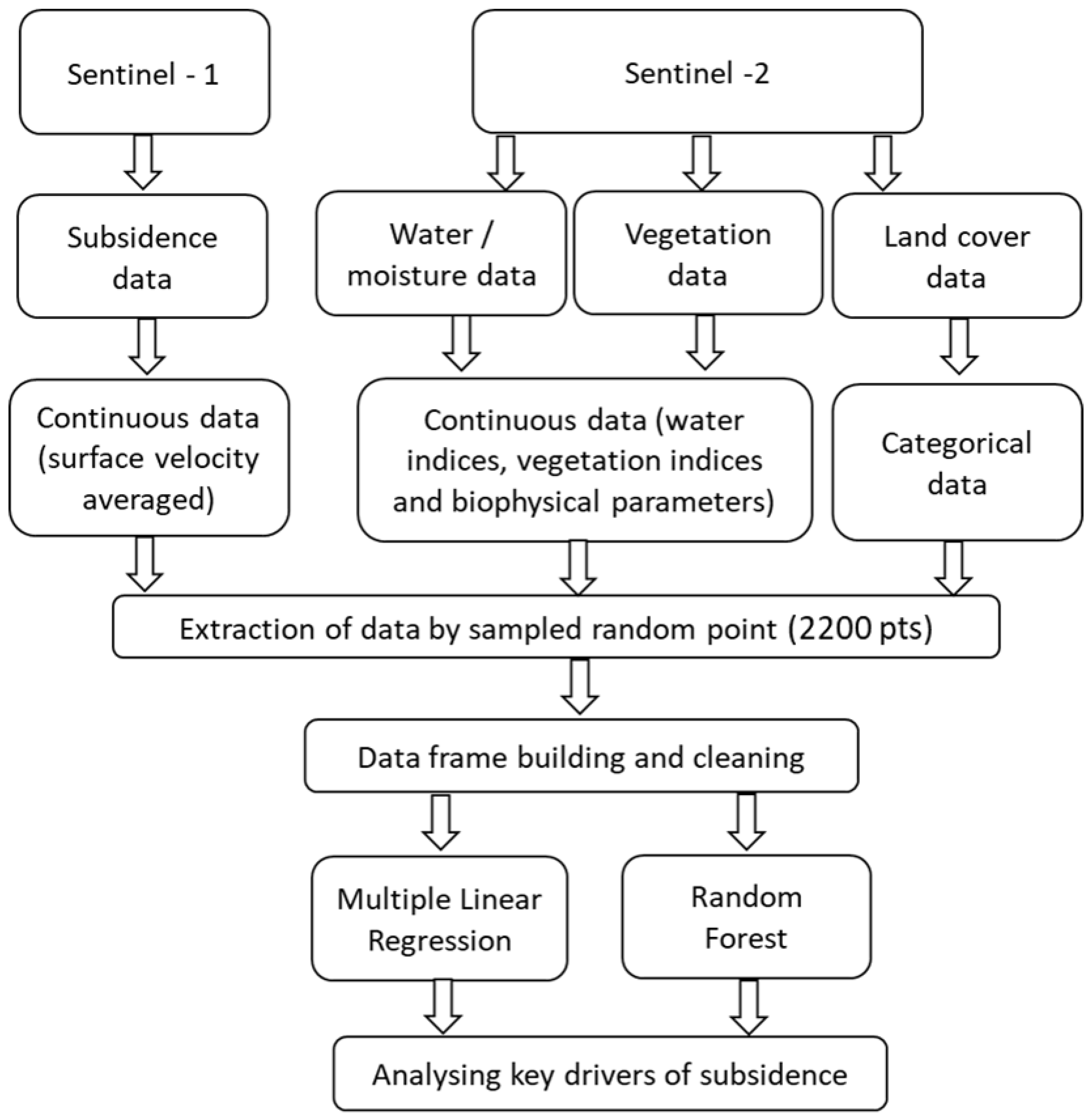
We used a big data approach to our investigation, sourcing and producing many remote sensing and GIS products that are relevant to tropical peat swamp forest subsidence and condition. We selected a linear (multiple linear regression) and non-linear (random forest regression) approach to investigate whether variance in subsidence rates across Selangor could be better explained by linear relationships or non-linear relationships. The variances and variable importance rankings from these model outputs were then compared to establish the key drivers of subsidence. This is summarised in our methodological approach (Figure 2). Image acquisition and pre-processing were the first steps for building different spatial layers; then, spectral indices and biophysical parameters were extracted to explain peat conditions.
Once we collated our suitable raster and vector dataset, we created 2200 random points covering all peatland areas in Selangor (see Figure 1). These random points were used as coordinates for extracting the values of each pixel of a given data layer. With this, we built a data frame of 2128 rows by 38 columns which was rescaled and used for running the analyses.

2.8.1. Multiple Linear Regression

Multiple Linear Regression (MLR) was carried out to investigate whether our independent variables could significantly predict tropical peat subsidence and to understand the spatial distribution of peat subsidence using a linear combination of our predictor variables. In this case, the dependent variable was the subsidence data, and the predictor variables were the spectral and vegetation variables.
MLR is defined as:
y = a + b1X1 + b2X2+ … + bnXn + ε
where y is the dependent variable, X are the predictors, n is the number of predictors, a is the intercept, b are the partial regression coefficients and ε is the estimated error.
RStudio was used to compute the MLR model using the function “lm” from the base package. The data was split 80:20 into training and test datasets and the MLR was conducted on the training set. F-statistics and the associated p-value were obtained for a given predictor and evaluated whether the association was significant between the predictor and the dependent variables. We obtained the R2 and the adjusted R2 for estimating the proportion of variance in the subsidence data that can be explained by the predictor variable values. Given that R2 is not penalised by the number of variables in the model, a better estimation of R2 is using the adjusted R2. Adjusted R2 was therefore used to determine the variance explained in the model. The residual standard error was also computed.
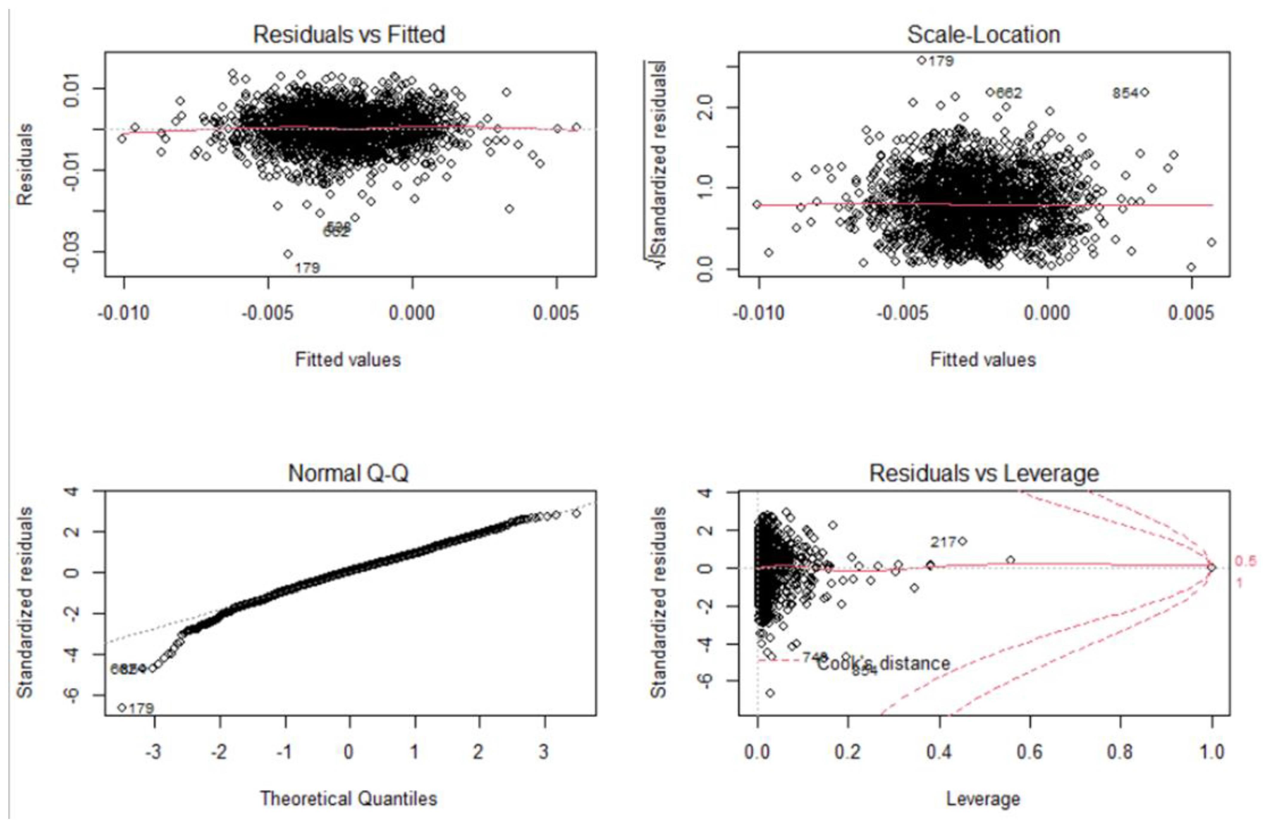
To select the best model, stepwise regression was used (also called stepwise selection) which involved removing and adding predictor variables until the best-performing model was found (based on the highest R2 value). For this, we used the “stepAIC” function from the MASS R package [48]. This function enabled computation of the stepwise regression using a combination of forward selection and backward elimination which eliminated collinearity in the data. In addition, variance inflation factors were computed to seek and eliminate any collinearity in the model. To ensure the model met the assumptions of univariate normality and homogeneity of variance, the residual plots were inspected (Figure A1).

2.8.2. Random Forest Regression

Random Forest Regression (RFR) is a machine learning algorithm and an alternative form of MLR. It is based on binary rule-based decisions (regression trees) and feature ranking that search for the optimal subset to explain how a predictor variable relates to a dependent variable [49]. RFR is a robust algorithm that can describe complex relationships and does not assume that the data has a particular distribution or linear relationship; therefore, it has been broadly used for understanding ecological and environmental systems [50,51,52,53]. The performance of the two models investigated was assessed based on model internally generated accuracy statistics and independent validation samples, calculating the RMSE of the predicted values and the correlation coefficient. Ten-fold cross-validation with five repetitions was computed in each model to guarantee model stability (non-overfit) and reliability [54].
RFR was carried out because it is a powerful feature selection method that scores the importance of the contribution of each variable towards explaining the dependent variable. The combination of MLR and RFR enabled an understanding of the variables that are most important for determining subsidence rates and the complex relationships in the data.
RFR was carried out in RStudio using the ‘randomForest’ package [49]. The functions within this package allowed for model tuning and analysis of the results, as well as the validation of the model. The dataset was split 80:20 into training and test datasets (the same data used for MLR). The most important parameters in RFR are the number of trees (500 as default) and the number of variables at each decision tree split (1/3 of the total number of variables) [55]. The first model was built using the default parameters and then this was tuned using the “tuneRF” function. This allowed us to search for the optimal number of variables used at each split (using the Out-of-bag error). Afterwards, the model was run eliminating the least important variable listed in the variable importance outputs at a time. This way, the best model was found based on the adjusted R2. Finally, the best models were validated with the test data (20% of the data) using the “predict” function from the ‘caret’ R Package [56]. RMSE was also calculated, as well as the correlation coefficient between the predicted and observed values.

3. Results

3.1. Patterns of APSIS Coherence and Subsidence

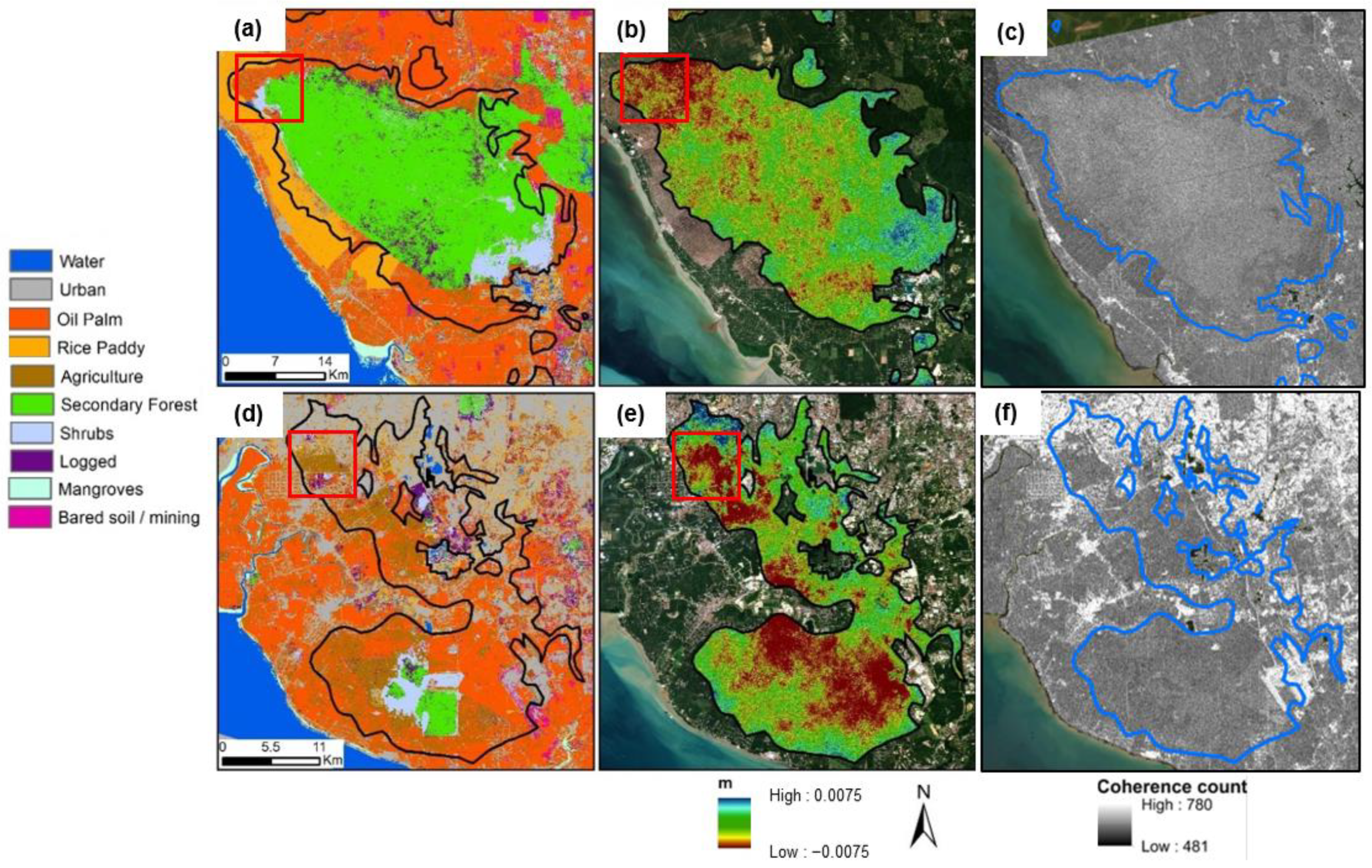
The overall coherence count, representing the number of coherent interferometric pairs per pixel, was highest in urban areas of Selangor due to the predominance of double-bounce scattering and low temporal decorrelation (Figure 3c,f). At both North Selangor and Kuala Langat, the overall coherence count of the secondary forest was moderate compared to oil palm, rice paddy and shrub land covers, which were overall lower. A moderate coherence count within the secondary forest land cover was likely achieved due to the presence of both surface water and tree trunks to enable double-bounce scattering and lower temporal decorrelation than expected overall. The coherence count maps show that an adequate number of coherent interferometric pairs (minimum 71) was achieved for every pixel using the APSIS method, enabling a reliable rate of deformation to be calculated for the entire region of Selangor.
When comparing subsidence rates across the study region, it was clear that subsidence was most pronounced in South Selangor (Figure 3e). Subsidence was also recorded in North Selangor but at a lower magnitude, particularly in the north part of the peatland (Figure 3b). Subsidence was present across all land cover categories except for bare soil in North Selangor. In some locations, land cover boundaries had a clear correspondence with patterns in subsidence (see red squares in Figure 3a,b,d,e), likely due to land cover change, forest clearance, and/or drainage (Figure 1).
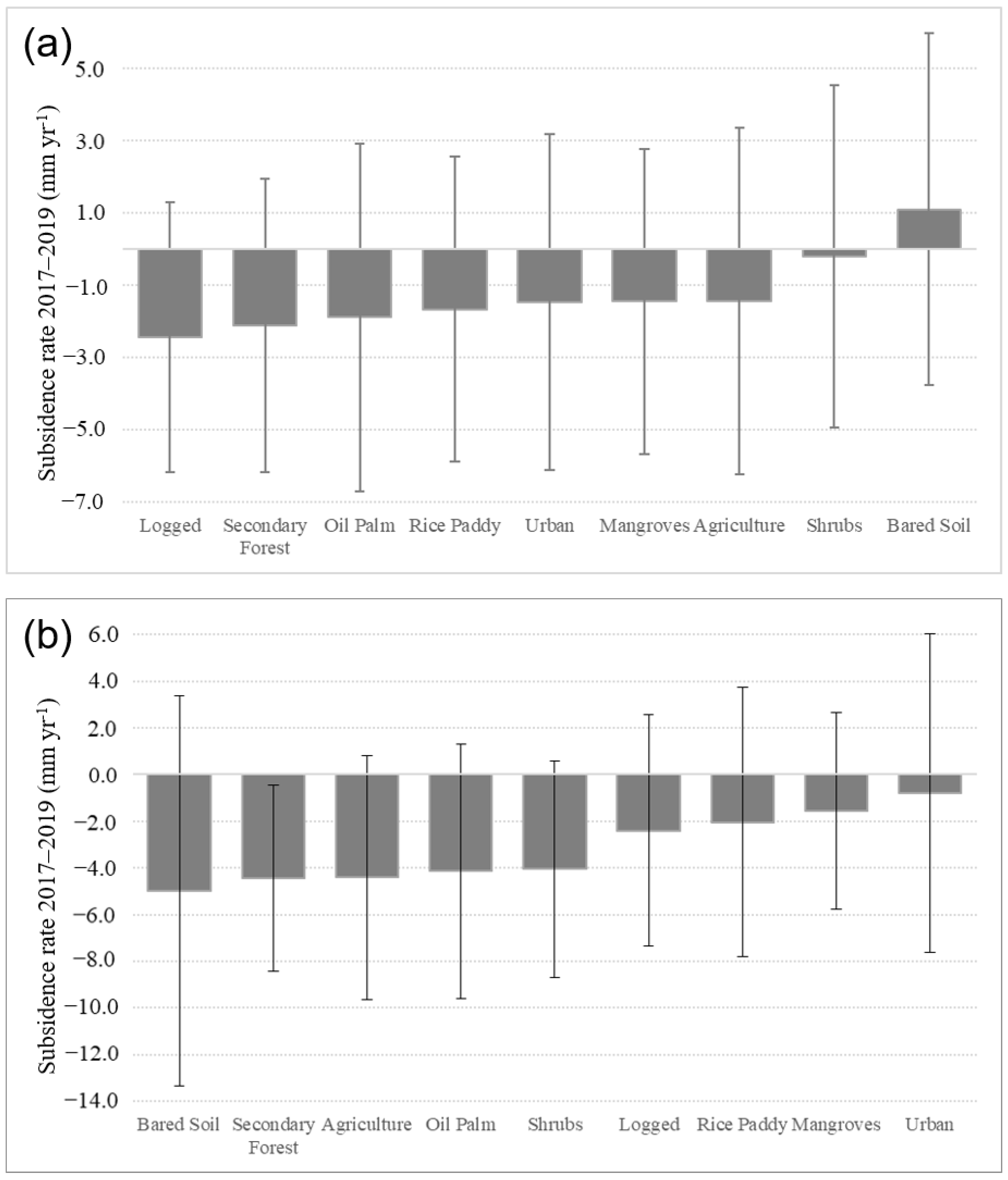
In South Selangor, subsidence occurred over extensive areas (~439 km2) with the greatest rates (of ca. −7.5 mm yr−1 between November 2017 and November 2019) occurring in areas with bare soil, secondary forest, oil palm plantations or agriculture (Figure 4). Forested areas in the centre of the peatland also showed subsidence but at a lower rate, suggesting that the impacts of drainage have expanded to reach areas which still have forest cover. In North Selangor, the higher rates of subsidence were more spatially confined and mainly found along the northern edge of the reserve. However, at North Selangor, relatively large central areas of the peatland seemed stable or at least much less impacted by subsidence (Figure 3b). Subsidence rates in bare soil showed opposing trends: bare soil in South Selangor was subsiding and North Selangor was uplifting.

3.2. Multiple Linear Regression

The MLR explained 13% of the variation in the ground motion (F = 5.73, p < 0.001). MLR results showed that the most significant variables (p-value: [0, 0.001]) for explaining subsidence were peat boundary distance (how far a given pixel is from the peat border) and land cover (mainly oil palm plantations and agriculture). This was followed by (p-value: [0.001, 0.01]) canal distance (how far a given pixel is from a canal or river), NDMI difference, and LAI_CW_2018. Finally, those variables with p-values of (0.01, 0.05] were EVI and MSI. p-values and significance can be found in Table A2 in Appendix A. A significant (99% confidence) correlation coefficient of 0.30 between the predicted values and the observed data with a RMSE = 0.0046 was found. The accuracy achieved in the validation was good considering the relatively low adjusted R2 of the model.
The MLR allowed us to understand the linear relationships between our predictor variables and the subsidence rate. However, given that tropical peatland subsidence is a complex environmental process and some of the non-linear relationships might be omitted in the MLR, we also performed RFR for its robustness and for its capability to find non-linear relationships in the data.

3.3. Random Forest Regression

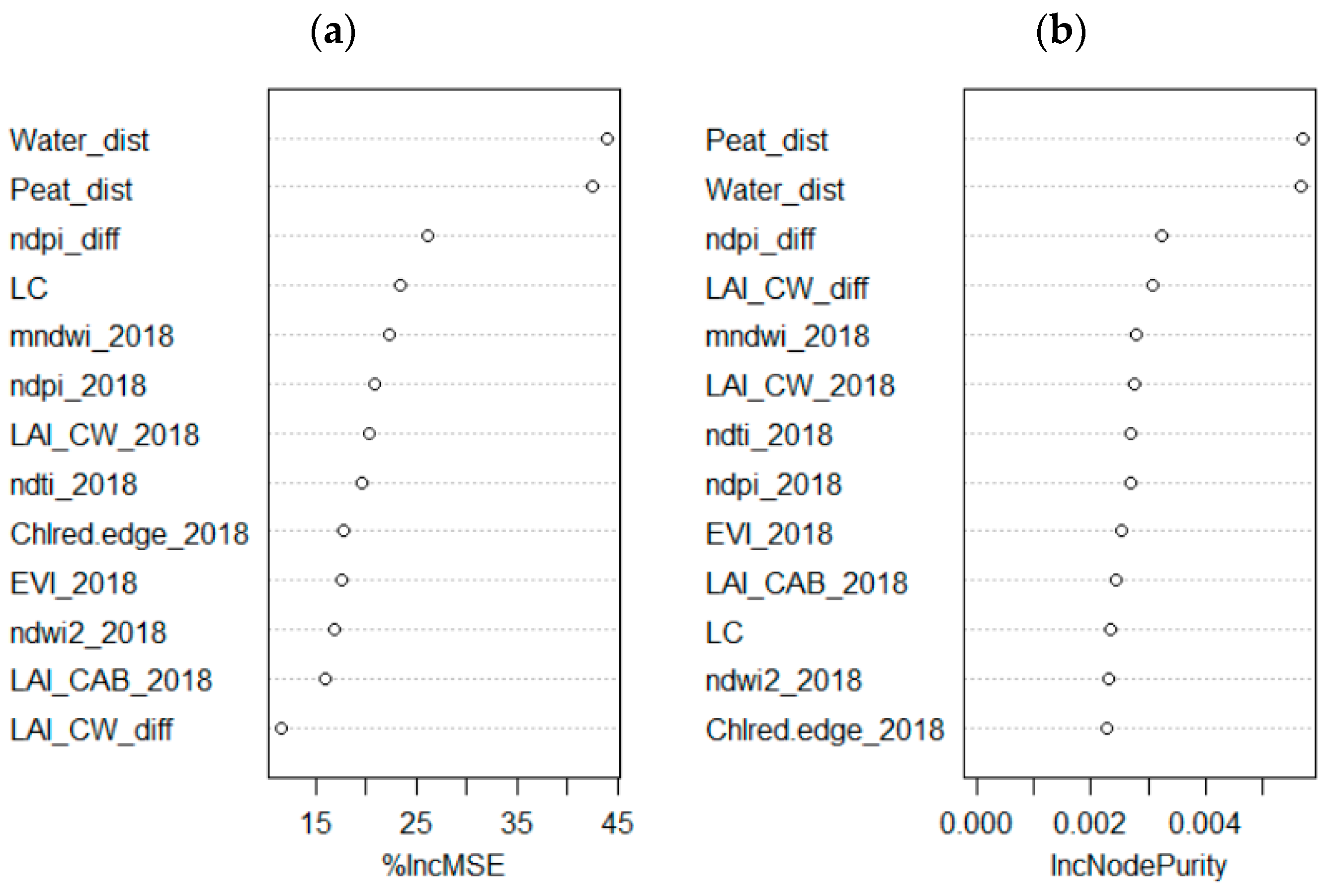
RFR was carried out using first the 37 variables and the default RFR parameters (i.e., 500 trees, and mtry = n/3). This produced a model that explained 20% of the variance which, after tuning the model (1000 trees and mtry = 37), increased marginally to 21.32%. The variable importance of this model is shown in Figure 5. The top three variables (canal distance, peat boundary distance, and presence of small ponds (ndpi)) were found in both variable importance measures: the percentage increase in MSE (%IncMSE) and the increase in node purity (IncNodePurity). The top three ranked variables for both variable importance measures were the same as in the results obtained in the MLR. In order to obtain the most parsimonious model with the highest accuracy, we tuned and ran the model iteratively by eliminating or adding one variable at a time and taking into account both the variable importance by %IncMSE and by IncNodePurity. Results of these iterations show that the best models performed with the 13 most important variables (%IncMSE) and with the 7 most important variables (IncNodePurity) (Figure 5, Table 2). With this, a selection of the most important variables was carried out, and finally, the best two models were computed, producing final results of 21.45% and 21.46% of variance explained by each of the models (%IncMSE and IncNodePurity, respectively). The summary of the results of all models is presented in Table 2.
The top 10 predictor variables which contributed most to the accuracy of subsidence mapping in Selangor are presented in Figure 5. The results reveal that both models included land cover, canal distance and peat boundary distance among the most important variables in all models. Some variables shown as driving factors in the top 10 for RFR were not present in the MLR (e.g., ChlredEdge Index, LAI_CW, GVMI, NDMI).

4. Discussion

4.1. Spatial and Temporal Patterns of Subsidence Rates for Selangor Peatlands

This study showed that widespread subsidence occurred across the major peatland areas in the Selangor region from 2017 to 2019. The maximum rate of subsidence reported by APSIS-DInSAR was −7.5 mm yr−1 over the 2017–2019 period, which was greater than the maximum subsidence rates of −5.8 mm yr−1 found in Arctic peatlands [31] and −6.2 mm yr−1 found in the Flow Country, Scotland [57], although lower than rates measured in another study from the Flow Country, Scotland (−11 mm yr−1 [28]). This rate was also considerably lower than point-based ground measurements from North Selangor, which measured a maximum rate of −25 mm yr−1 using subsidence poles [47], indicating that APSIS-DInSAR rates are an underestimation. With this underestimation in mind, we continue to discuss temporal and spatial patterns of subsidence in relative terms and contextually with an understanding of the site.
Overall, higher subsidence rates were seen at the edges of the peat where agricultural activities have rapidly expanded, including rice paddies and smallholder oil palm [40]. Subsidence was most severe in South Selangor, where the highest subsidence rates were documented both within the peat dome and at the peat boundary. This corresponds with results from Marshall et al. [30], which showed high subsidence around Kuala Lumpur airport which extended into the peatland. It was clear that the impacts of land use change were not constrained to the production areas, i.e., if one part of the peatland is drained, the effects are noticeable across the wider peatland hydrological unit (Figure 3). This is a particularly important point to note for policy makers and land managers when making decisions on peatland management and offers a strong argument for ensuring high water table levels across wider areas beyond the peat swamp forest, for example, by implementing a buffer zone whereby no drainage is permitted around peat swamp forest reserves if there is an overarching aim of conservation and protection.
The continued low-rate subsidence of the interior of the North Selangor forest reserve two decades after the cessation of logging and drainage ditch digging shows that the peatland has not yet reached a stable equilibrium [58]. It also implies that the recovery of these forests and the recommencement of peat formation is slow, especially if the hydrological integrity of the peatland is not fully restored since remnant drainage canals continue to drain the water table and hinder the recovery of these peat swamp forests [59,60,61]. The widespread occurrence of subsidence is also a concern as it suggests loss of peat soil and its water holding capacity, increased risk of flooding and thereby the potential long-term loss of neighbouring agricultural production as well as ecosystem recovery [62,63]. Although some areas of North Selangor had not yet fully recovered, it was also clear that subsidence rates of large tracts of the interior of the peatlands had levelled off and stabilised with time since gazettement in 1990, as seen in other studies [64,65]. As such, documented rates of uplift from InSAR may be due to the rebound of the peat surface due to groundwater recharge [66,67].

4.2. Variable Importance

Despite the spatial and temporal complexity of peat subsidence, this study showed that remotely sensed products descriptive of peatland geography, the peat surface and above-ground biomass can explain up to 21.5% of the variance (Table 2). This offers insights into the most relatively important processes that control subsidence at the landscape scale: peat boundary distance, land cover and canal distance. Water spectral indices were also ranked as important, highlighting the need to maintain the hydrological function of tropical peat to avoid subsidence.
Geographical variables such as peat boundary distance, land cover and canal distance were consistently the most important variables for describing spatial patterns of subsidence across Selangor. The high importance of these variables can partly be explained by the linearity between the subsidence rate and the depth of the peat and water table as found by Ritzema et al. [19]. Peat boundary distance, in particular, has a strong relationship with peat depth and water table level; the further the distance from the peat boundary, the deeper the peat, but the lower the water table due to the increased lateral flow away from the centre of the dome [58,68]. This therefore results in overall increased subsidence rates towards the centre of the dome, particularly in areas impacted by drainage enhancing the impact of lateral water flow out of the peatland, and with increased distance from the peat boundary.
Land cover and canal distance likely had an interacting and compounding effect on subsidence rates in Selangor. Land cover changes dictate peat subsidence rates [65], whereby the conversion of tropical peat swamp forests involves logging and drainage, deepening water table levels and inducing subsidence as a result. In SE Asia, agricultural conversion of peatlands has accelerated over time; between 2007 and 2015, industrial oil palm plantations almost doubled their coverage over SE Asian tropical peatlands, covering 27% of all SE Asian peatlands in 2015. Additionally, smallholder plantations covered 22% of all peatlands in the same year [9]. This rate of conversion applies to Selangor, where the encroachment of oil palm agriculture in particular led to mass logging and drainage of peatland, most notably in South Selangor (Figure 3d). Such land cover changes in Selangor have resulted in the digging of ditches and canals to drain the peatland. The greatest subsidence rates were seen closest to canals and ditches, with a parabolic-shaped relationship with distance from the canal [64]. The strength of this relationship in Selangor was reflected in the importance of both canal distance and land use in the MLR and RFR models.

4.3. Effectiveness of APSIS-DInSAR and Modelling Techniques

C-band InSAR phase unwrapping can fail to produce an accurate vertical displacement measurement if a well-defined fringe pattern is absent from any interferogram, which is likely over an intermittently coherent area such as a peat swamp forest [30]. DInSAR methods also have poor capability for measuring rapid surface deformation rates [69]. If surface deformation exceeds one-quarter of a wavelength between a pair of images, the magnitude and direction of motion cannot be confidently determined, leading to suppressed variations in time series, especially with long temporal baselines [70,71]. This has been previously recorded in North Selangor, with a surface level change of 18.5 mm documented within a Sentinel-1 revisit period of 12 days [47]. Both scenarios outlined result in an underestimation of subsidence rates. Based on the likelihood of phase unwrapping errors over these sites, and the comparison of measurements from the ground at North Selangor and elsewhere, we believe that the subsidence rates determined by APSIS-DInSAR in this study are underestimates and should be considered with caution. As such, we propose a selection of appropriate and inappropriate applications of the method at present towards tropical peatland conservation, restoration and management in Table 3.
Our study demonstrated that ASPIS-DInSAR had sufficient coherence over peat swamp forests in line with previous findings in North Selangor [37] and South Selangor [30]. Out of the two models we used for assessing how other remotely sensed peatland properties related to the ground motion data, the RFR model explained greater variance of the spatial patterns of subsidence (21.5%) compared to the MLR model (13%). This can be attributed to the fact that RFR is a machine learning model that accounts for non-linear relationships between subsidence and the explanatory variables. As such, RFR is recommended for use when exploring peat swamp forest characteristics with big data. In addition, RFR is capable of selecting important spectral and environmental features that are sensitive to subsidence data and improves the accuracy levels for understanding and predicting subsidence across the space. Despite the poorer performance of the MLR model, RFR was only able to account for 8.5% more variance explained. The use of MLR therefore showed the extent to which linear relationships between tropical peat subsidence and above-ground peat swamp forest variables exist. This further highlights the complexity of the relationships between subsidence and its predictive variables.

4.4. Recommended Further Work

This study highlights the potential of remote sensing data for mapping peat subsidence properties, both at local and regional scales. However, it is crucial to acknowledge the limitations and complexity of peat subsidence and the potential challenges associated with interpreting remote sensing data through machine learning techniques. Overall, the dynamism and spatial variability of peat properties, the heterogeneity of the landscape, the varied practices for agriculture and water management, and the lack of ground measurements of subsidence and peat profile-specific datasets that can be acquired through remotely sensed data (e.g., bulk density, peat depth) are among the sources of limitation on model performance. We managed to explain only a proportion of the variance of such a complex process; the performance of the models could be improved upon by collecting more ground data on variables that describe peat profile condition and water table level directly and incorporating this into the model, rather than including variables that describe the peat surface and above-ground biomass characteristics from remote sensing products only. Time series data of surface subsidence and water table levels from Evans et al. [72] presented a strong relationship between peat surface level and water table level. This illustrates the importance of including a product that directly reflects water table levels across Selangor peatlands in subsidence models. Indeed, the importance of MNDWI, an indicator of surface water presence, as a variable in the RFR models, highlights the importance of water levels as an explanatory variable for landscape level patterns in subsidence.
Time series analysis of subsidence rates and changes in tropical peat swamp forest characteristics and land cover could also improve the amount of variance explained in the models. The APSIS technique is able to provide a time series product, whereby a time series of surface elevation change is produced with observations that match the satellite acquisition frequency (12 days for Sentinel-1 at low latitudes) after the launch of parallel satellite Sentinel-1C scheduled for 2024. Patterns in magnitude and frequency of seasonal surface motion can be derived from the time series, which acts as a proxy for peat conditions [57,73,74]. Such an approach could provide regional-scale information on peat profile condition, a missing component of the models presented in this study. The work of Bradley et al. [74] and Marshall et al. [57] has shown a greater benefit in terms of mapping peat condition trends with the time series produced from the APSIS technique rather than the average vertical velocity, therefore future work should seek to make use of the time series output instead. Ground-based technologies have also improved significantly, with the introduction of automated monitoring systems for peat surface motion [72], potentially enabling improved comparisons between methods in the future. Further, our results indicate that a considerable component of the variation in ground motion was driven by below-surface variables such as water table level and peat properties, e.g., bulk density, elasticity, and peat depth, which are currently not observable with satellite data, and which most likely explain the relatively low predictive capability of the model.
Despite the APSIS-DInSAR subsidence underestimation documented in this study, there is great potential for the APSIS-DInSAR approach to be further developed for flood risk prediction and monitoring linked to the predicted flood and drainability outcomes in Sarawak [14]. This method also has the potential to contribute towards adherence monitoring for the new Round Table on Sustainable Palm Oil (RSPO) guidance on drainability and subsidence surveying, a new requirement for all RSPO peat plantations to optimise the peat condition and therefore the lifetime of these plantations [75]. We hope that with further work to improve the modelling of subsidence rates and peat conditions, the APSIS-DInSAR method can aid in understanding the consequences of drainage on tropical peatland conditions and subsidence and inform management strategies towards restoring these environments.

Author Contributions

B.d.l.B.-B.: performed the data collection, computed results and analysis, wrote the manuscript; M.J.L.: performed the data collection and analysis of the results, wrote the manuscript; S.S.: conceived the study, provided advice on the data analysis, supervision and wrote the manuscript; D.S.B.: conceived the study, supervision, provided advice on the data analysis; D.G.: computed results; A.S.: conceived the study, provided advice on the data analysis; B.C.: data collection and understanding; S.E.P.: conceived the study, supervision; D.J.L.: conceived the study, supervision; C.D.E.: conceived the study, supervision; K.J.T.: conceived the study, supervision; S.E.: conceived the study, supervision. B.d.l.B.-B. and M.J.L. contributed equally to this work. All authors have read and agreed to the published version of the manuscript.

Funding

This work is part of the Peatland Assessment in SE Asia by Satellite (PASSES) project funded by the United Kingdom Space Agency (UKSA) and delivered by a consortium of CGI IT UK Ltd., Terra Motion, United Kingdom Centre for Ecology and Hydrology, Liverpool John Moores University, University of Nottingham and University of Leicester, in partnership with the Global Environment Centre (GEC) of Malaysia. This work was also supported by a Natural Environment Research Council (NERC) and Biotechnology and Biological Sciences Research Council (BBSRC) PhD studentship as part of the STARS Doctoral Training Partnership [NE/M009106/1].

Data Availability Statement

The raw data supporting the conclusions of this article will be made available by the authors on request.

Acknowledgments

The authors would like to acknowledge: (1) the UK Space Agency for providing financial support for conducting this research through the IPP call 2 supporting the PASSES project; (2) Terra Motion for providing subsidence data, (3) the Copernicus Programme for the availability and use of Sentinel-1 and Sentinel-2 data.

Conflicts of Interest

Authors David Gee and Andrew Sowter were employed by the company Terra Motion Limited. The remaining authors declare that the research was conducted in the absence of any commercial or financial relationships that could be construed as a potential conflict of interest.

Appendix A

Table A1. Formulae for deriving spectral indices used in analysis.
IndexFormulaDefinitionReference
Normalized Difference Vegetation IndexNDVI = (B12 − B8)/(B12 + B8)Detection of live green vegetation and an indicator of its condition. Chlorophyll sensitive.[76]
Modified Normalized Difference Water IndexMNDWI = (B9 − B12)/(B9 + B12)Enhances surface water features whilst supressing or removing noise from vegetation, soil and urban areas.[77]
Enhanced Vegetation IndexEVI = 2.5 × (B8 − B4)/((B8 + 6.0 × B4 − 7.5 × B2) + 1.0))Detection of live green vegetation with increased sensitivity in high biomass regions. More sensitive to canopy structural variations than NDVI.[78]
Normalized Difference Pond IndexNDPI = (B11 − B3)/(B11 + B3)Distinguishes small ponds from water bodies and differentiates vegetation within ponds from their surroundings.[79]
Normalized Difference Turbidity IndexNDTI = (B4 − B3)/(B4 + B3)A measure of the amount of suspended sediments. Therefore, a measure of the clarity of a water body.[79]
Normalized Difference Water IndexNDWI = (B8 − B12)/(B8 + B12)Sensitive to the liquid water content of vegetation canopies. Less sensitive to atmospheric effects than NDVI.[80]
Normalized Difference Water Index 2NDWI2 = (B3 − B8)/(B3 + B8)Detects surface water presence in wetland environments and allows for measurement of surface water extent.[81]
Chlorophyll Red Edge IndexChlredEdge = (B7/B5) − 1High reflectance of vegetation in the NIR region. Used to estimate plant composition, including chlorophyll content of leaves.[82]
Global Vegetation Moisture IndexGVMI = (B9 + 0.1) − (B12 + 0.02)/(B9 + 0.1) + (B12 + 0.02)Vegetation water content at the canopy level.[83]
Moisture Stress IndexMSI = B11/B8Sensitive to increases in leaf water content. Applications include fire hazard analysis and canopy stress analysis. [84]
Normalised Burn RatioNBR = (B8 − B12)/(B8 + B12)Identifies burned areas and provides a measure of burn severity.[85]
Normalized Difference Moisture IndexNDMI = (B8 − B11)/(B8 + B11)Sensitive to moisture levels in vegetation. Used to monitor droughts and fuel provision in high-risk fire zones.[86]
Figure A1. Residual plots for multiple regression.
Remotesensing 16 02249 g0a1
Table A2. p-values and significance of multiple linear regression models. Bold values represent significance below threshold of 0.05.
PredictorsEstimatesCIp
(Intercept)−0.00−0.00–−0.000.023
LC [2]−0.00−0.00–−0.00<0.001
LC [3]−0.00−0.00–0.000.346
LC [4]−0.00−0.00–−0.00<0.001
LC [5]−0.00−0.00–0.000.843
LC [6]0.00−0.00–0.000.298
LC [7]−0.00−0.00–0.000.054
LC [8]0.00−0.01–0.010.701
LC [9]0.00−0.00–0.000.927
Peat dist−0.00−0.00–−0.00<0.001
Water dist−0.00−0.00–−0.000.008
mndwi diff0.00−0.00–0.000.921
ndpi diff0.00−0.00–0.000.075
ndti diff−0.00−0.00–0.000.501
ndwi diff−0.00−0.00–0.000.742
ndwi2 diff0.00−0.00–0.000.939
ChlredEdge diff−0.00−0.00–0.000.088
EVI diff−0.00−0.00–0.000.141
GVMI diff0.00−0.00–0.000.072
NDVI diff−0.00−0.00–0.000.145
MSI diff0.000.00–0.000.011
NBR diff−0.00−0.01–0.000.500
NDMI diff0.000.00–0.010.001
FAPAR diff−0.00−0.00–0.000.750
FCOVER diff0.00−0.00–0.000.231
LAI diff0.00−0.00–0.000.461
LAI CAB diff−0.00−0.00–0.000.084
LAI CW diff−0.00−0.00–−0.000.021
Chlred edge 2018−0.00−0.00–0.000.133
EVI 2018−0.00−0.00–−0.000.016
GVMI 20180.00−0.00–0.010.606
NDVI 2018−0.00−0.01–0.000.419
MSI 20180.00−0.00–0.000.935
NBR 2018−0.10−0.21–0.010.067
NDMI 20180.00−0.00–0.010.155
FAPAR 20180.00−0.00–0.000.898
FCOVER 20180.00−0.00–0.010.353
LAI 2018−0.00−0.00–0.000.227
LAI CAB 20180.00−0.00–0.000.817
LAI CW 2018−0.00−0.00–−0.000.006
mndwi 20180.00−0.00 – 0.000.422
ndpi 2018−0.00−0.00–0.000.807
ndti 2018−0.00−0.00–0.000.322
ndwi 20180.09−0.01–0.200.083
ndwi2 2018−0.00−0.01–0.000.456
Observation number2113
R2/R2 adjusted0.129/0.110

References

  1. Xu, J.; Morris, P.J.; Liu, J.; Holden, J. PEATMAP: Refining estimates of global peatland distribution based on a meta-analysis. Catena 2018, 160, 134–140. [Google Scholar] [CrossRef]
  2. Wösten, J.H.; Van Den Berg, J.; Van Eijk, P.; Gevers, G.J.; Giesen, W.B.; Hooijer, A.; Idris, A.; Leenman, P.H.; Rais, D.S.; Siderius, C.; et al. Interrelationships between hydrology and ecology in fire degraded tropical peat swamp forests. Water Resour. Dev. 2006, 22, 157–174. [Google Scholar] [CrossRef]
  3. Cooper, H.V.; Evers, S.; Aplin, P.; Crout, N.; Dahalan, M.P.; Sjogersten, S. Greenhouse gas emissions resulting from conversion of peat swamp forest to oil palm plantation. Nat. Commun. 2020, 11, 407. [Google Scholar] [CrossRef] [PubMed]
  4. Gorham, E. Northern peatlands: Role in the carbon cycle and probable responses to climatic warming. Ecol. Appl. 1991, 1, 182–195. [Google Scholar] [CrossRef] [PubMed]
  5. Lappalainen, E. Global Peat Resources; International Peat Society: Jyväskylä, Finland, 1996; ISBN 952-90-7487-5. TRN: 980200439. [Google Scholar]
  6. Page, S.E.; Rieley, J.O.; Banks, C.J. Global and regional importance of the tropical peatland carbon pool. Glob. Change Biol. 2011, 17, 798–818. [Google Scholar] [CrossRef]
  7. IPCC. Climate Change 2022: Impacts, Adaptation, and Vulnerability. Contribution of Working Group II to the Sixth Assessment Report of the Intergovernmental Panel on Climate Change; Pörtner, H.-O., Roberts, D.C., Tignor, M., Poloczanska, E.S., Mintenbeck, K., Alegría, A., Craig, M., Langsdorf, S., Löschke, S., Möller, V., et al., Eds.; Cambridge University Press: Cambridge, UK; New York, NY, USA, 2022; p. 3056. [Google Scholar] [CrossRef]
  8. Leifeld, J.; Menichetti, L. The underappreciated potential of peatlands in global climate change mitigation strategies. Nat. Commun. 2018, 9, 1071. [Google Scholar] [CrossRef]
  9. Miettinen, J.; Chenghua, S.; Liew, S.C. Land cover distribution in the peatlands of Peninsular Malaysia, Sumatra and Borneo in 2015 with changes since 1990. Glob. Ecol. Conserv. 2016, 6, 67–78. [Google Scholar] [CrossRef]
  10. Ribeiro, K.; Pacheco, F.S.; Ferreira, J.W.; de Sousa-Neto, E.R.; Hastie, A.; Krieger Filho, G.C.; Alvalá, P.C.; Forti, M.C.; Ometto, J.P. Tropical peatlands and their contribution to the global carbon cycle and climate change. Glob. Change Biol. 2021, 27, 489–505. [Google Scholar] [CrossRef]
  11. Hooijer, A.; Page, S.; Jauhiainen, J.; Lee, W.A.; Lu, X.X.; Idris, A.; Anshari, G. Subsidence and carbon loss in drained tropical peatlands. Biogeosciences 2012, 9, 1053–1071. [Google Scholar] [CrossRef]
  12. Evans, C.D.; Williamson, J.M.; Kacaribu, F.; Irawan, D.; Suardiwerianto, Y.; Hidayat, M.F.; Laurén, A.; Page, S.E. Rates and spatial variability of peat subsidence in an Indonesian plantation landscape. Geoderma 2018, 338, 410–421. [Google Scholar] [CrossRef]
  13. Hoyt, A.M.; Chaussard, E.; Seppalainen, S.S.; Harvey, C.F. Widespread subsidence and carbon emissions across Southeast Asian peatlands. Nat. Geosci. 2020, 13, 435–440. [Google Scholar] [CrossRef]
  14. Deltares. Flooding Projections from Elevation and Subsidence Models for Oil Palm Plantations in the Rajang Delta Peatlands, Sarawak, Malaysia. 2015. Available online: https://cms.deltares.nl/assets/common/downloads/Rajang-Delta-Peatland-Subsidence-Flooding-Deltares-2015.pdf (accessed on 16 June 2024).
  15. Girkin, N.T.; Dhandapani, S.; Evers, S.; Ostle, N.; Turner, B.L.; Sjögersten, S. Interactions between labile carbon, temperature and land use regulate carbon dioxide and methane production in tropical peat. Biogeochemistry 2020, 147, 87–97. [Google Scholar] [CrossRef]
  16. Page, S.; Hosciło, A.; Wösten, H.; Jauhiainen, J.; Silvius, M.; Rieley, J.; Ritzema, H.; Tansey, K.; Graham, L.; Vasander, H.; et al. Restoration ecology of lowland tropical peatlands in Southeast Asia: Current knowledge and future research directions. Ecosystems 2009, 12, 888–905. [Google Scholar] [CrossRef]
  17. Ritzema, H.; Grobbe, T.; Chong, T.; Wösten, J.H.M. Decision support system for peatland management in the humid tropics. In Proceedings of the 9th International Drainage Workshop, Utrecht, The Netherlands, 10–13 September 2003. [Google Scholar]
  18. Ritzema, H.; Wösten, H. Hydrology of Borneo’s peat swamps. In Strategies for implementing sustainable management of peatlands in Borneo. In Proceedings of the STRAPEAT Partners Workshop, Palangka Raya, Kalimantan, Indonesia and Sibu, Sarawak, Malaysia, 30 March–5 April 2002. [Google Scholar]
  19. Ritzema, H.; Limin, S.; Kusin, K.; Jauhiainen, J.; Wösten, H. Canal blocking strategies for hydrological restoration of degraded tropical peatlands in Central Kalimantan, Indonesia. Catena 2014, 114, 11–20. [Google Scholar] [CrossRef]
  20. Ritzema, H. Main drainage systems. In MSc Programme Land and Water Development for Food Security; UNESCO-IHE: Delft, The Netherlands, 2014. [Google Scholar]
  21. Tan, Z.U.; Lupascu, M.; Wijedasa, L.S. Paludiculture as a sustainable land use alternative for tropical peatlands: A review. Sci. Total Environ. 2020, 753, 142111. [Google Scholar] [CrossRef] [PubMed]
  22. FAO. Peatlands Mapping and Monitoring—Recommendations and Technical Overview; FAO: Rome, Italy, 2020. [Google Scholar] [CrossRef]
  23. Lu, Z.; Crane, M.; Kwoun, O.I.; Wells, C.; Swarzenski, C.; Rykhus, R. C-band radar observes water level change in swamp forests. EOS Trans. Am. Geophys. Union 2005, 86, 141–144. [Google Scholar] [CrossRef]
  24. Mohammadimanesh, F.; Salehi, B.; Mahdianpari, M.; Brisco, B.; Motagh, M. Wetland water level monitoring using interferometric synthetic aperture radar (InSAR): A review. Can. J. Remote Sens. 2018, 44, 247–262. [Google Scholar] [CrossRef]
  25. Zhou, X.; Chang, N.B.; Li, S. Applications of SAR interferometry in earth and environmental science research. Sensors 2009, 9, 1876–1912. [Google Scholar] [CrossRef]
  26. Kim, S.W.; Wdowinski, S.; Amelung, F.; Dixon, T.H.; Won, J.S. Interferometric coherence analysis of the Everglades wetlands, South Florida. IEEE Trans. Geosci. Remote Sens. 2013, 51, 5210–5224. [Google Scholar] [CrossRef]
  27. Pepe, A.; Calò, F. A review of interferometric synthetic aperture RADAR (InSAR) multi-track approaches for the retrieval of Earth’s surface displacements. Appl. Sci. 2017, 7, 1264. [Google Scholar] [CrossRef]
  28. Alshammari, L.; Large, D.J.; Boyd, D.S.; Sowter, A.; Anderson, R.; Andersen, R.; Marsh, S. Long-term peatland condition assessment via surface motion monitoring using the ISBAS DInSAR technique over the Flow Country, Scotland. Remote Sens. 2018, 10, 1103. [Google Scholar] [CrossRef]
  29. Cigna, F.; Sowter, A. The relationship between intermittent coherence and precision of ISBAS InSAR ground motion velocities: ERS-1/2 case studies in the UK. Remote Sens. Environ. 2017, 202, 177–198. [Google Scholar] [CrossRef]
  30. Marshall, C.; Large, D.J.; Athab, A.; Evers, S.L.; Sowter, A.; Marsh, S.; Sjögersten, S. Monitoring tropical peat related settlement using ISBAS InSAR, Kuala Lumpur International Airport (KLIA). Eng. Geol. 2018, 244, 57–65. [Google Scholar] [CrossRef]
  31. De la Barreda-Bautista, B.; Boyd, D.S.; Ledger, M.; Siewert, M.B.; Chandler, C.; Bradley, A.V.; Gee, D.; Large, D.J.; Olofsson, J.; Sowter, A.; et al. Towards a Monitoring Approach for Understanding Permafrost Degradation and Linked Subsidence in Arctic Peatlands. Remote Sens. 2022, 14, 444. [Google Scholar] [CrossRef]
  32. Gee, D.; Sowter, A.; Grebby, S.; de Lange, G.; Athab, A.; Marsh, S. National geohazards mapping in Europe: Interferometric analysis of the Netherlands. Eng. Geol. 2019, 256, 1–22. [Google Scholar] [CrossRef]
  33. Gee, D.; Bateson, L.; Grebby, S.; Novellino, A.; Sowter, A.; Wyatt, L.; Marsh, S.; Morgenstern, R.; Athab, A. Modelling groundwater rebound in recently abandoned coalfields using DInSAR. Remote Sens. Environ. 2020, 249, 112021. [Google Scholar] [CrossRef]
  34. Kasischke, E.S.; Bourgeau-Chavez, L.L. Monitoring South Florida wetlands using ERS-1 SAR imagery. Photogramm. Eng. Remote Sens. 1997, 63, 281–291. [Google Scholar]
  35. Brisco, B.; Ahern, F.; Hong, S.H.; Wdowinski, S.; Murnaghan, K.; White, L.; Atwood, D.K. Polarimetric decompositions of temperate wetlands at C-band. IEEE J. Sel. Top. Appl. Earth Obs. Remote Sens. 2015, 8, 3585–3594. [Google Scholar] [CrossRef]
  36. Tsyganskaya, V.; Martinis, S.; Marzahn, P.; Ludwig, R. Detection of temporary flooded vegetation using Sentinel-1 time series data. Remote Sens. 2018, 10, 1286. [Google Scholar] [CrossRef]
  37. Ledger, M.J.; Sowter, A.; Morrison, K.; Evans, C.D.; Large, D.J.; Athab, A.; Gee, D.; Brown, C.; Sjögersten, S. Potential of APSIS-InSAR for measuring surface oscillations of tropical peatlands. PLoS ONE 2024, 19, e0298939. [Google Scholar] [CrossRef]
  38. Wong, C.L.; Liew, J.; Yusop, Z.; Ismail, T.; Venneker, R.; Uhlenbrook, S. Rainfall characteristics and regionalization in Peninsular Malaysia based on a high resolution gridded data set. Water 2016, 8, 500. [Google Scholar] [CrossRef]
  39. Parish, F.; Dahalan, M.; Rahim, H. Integrated Management Plan for North Selangor Peat Swamp Forest 2014–2023 for Selangor State Forestry Department; Draft (30 June 2014) Revision, 2; Global Climate Action Partnership: Denver, CO, USA, 2014. [Google Scholar]
  40. Charters, L.J.; Aplin, P.; Marston, C.G.; Padfield, R.; Rengasamy, N.; Bin Dahalan, M.P.; Evers, S. Peat swamp forest conservation withstands pervasive land conversion to oil palm plantation in North Selangor, Malaysia. Int. J. Remote Sens. 2019, 40, 7409–7438. [Google Scholar] [CrossRef]
  41. Brown, C.; Boyd, D.S.; Sjögersten, S.; Clewley, D.; Evers, S.L.; Aplin, P. Tropical peatland vegetation structure and biomass: Optimal exploitation of airborne laser scanning. Remote Sens. 2018, 10, 671. [Google Scholar] [CrossRef]
  42. Gorelick, N.; Hancher, M.; Dixon, M.; Ilyushchenko, S.; Thau, D.; Moore, R. Google Earth Engine: Planetary-scale geospatial analysis for everyone. Remote Sens. Environ. 2017, 202, 18–27. [Google Scholar] [CrossRef]
  43. Hijmans, R.J.; van Etten, J. Raster: Geographic Analysis and Modelling with Raster Data. R Package Version 2.0-12. 2012. Available online: http://CRAN.R-project.org/package=raster (accessed on 20 March 2020).
  44. Sowter, A.; Bateson, L.; Strange, P.; Ambrose, K.; Syafiudin, M.F. DInSAR estimation of land motion using intermittent coherence with application to the South Derbyshire and Leicestershire coalfields. Remote Sens. Lett. 2013, 4, 979–987. [Google Scholar] [CrossRef]
  45. Sowter, A.; Amat, M.B.C.; Cigna, F.; Marsh, S.; Athab, A.; Alshammari, L. Mexico City land subsidence in 2014–2015 with Sentinel-1 IW TOPS: Results using the Intermittent SBAS (ISBAS) technique. Int. J. Appl. Earth Obs. Geoinf. 2016, 52, 230–242. [Google Scholar] [CrossRef]
  46. Ledger, M.J. Monitoring Surface Oscillation Dynamics of Tropical Peatlands: A Novel Approach Using APSIS-InSAR. Ph.D. Thesis, University of Nottingham, Nottingham, UK, 2022. [Google Scholar]
  47. Ledger, M.J.; Evans, C.D.; Large, D.J.; Evers, S.; Brown, C.; Jovani-Sancho, A.J.; Callaghan, N.; Vane, C.H.; Marshall, C.; Baskaran, A.; et al. Tropical peat surface oscillations are a function of peat condition at North Selangor peat swamp forest, Malaysia. Front. Environ. Sci. 2023, 11, 1182100. [Google Scholar] [CrossRef]
  48. Ripley, B.; Venables, B.; Bates, D.M.; Hornik, K.; Gebhardt, A.; Firth, D.; Ripley, M.B. Package ‘mass’. Cran R 2013, 538, 113–120. [Google Scholar]
  49. Breiman, L. Random forests. Mach. Learn. 2001, 45, 5–32. [Google Scholar] [CrossRef]
  50. Brown, M.E.; Lary, D.J.; Vrieling, A.; Stathakis, D.; Mussa, H. Neural networks as a tool for constructing continuous NDVI time series from AVHRR and MODIS. Int. J. Remote Sens. 2008, 29, 7141–7158. [Google Scholar] [CrossRef]
  51. Fu, B.; Wang, Y.; Campbell, A.; Li, Y.; Zhang, B.; Yin, S.; Xing, Z.; Jin, X. Comparison of object-based and pixel-based Random Forest algorithm for wetland vegetation mapping using high spatial resolution GF-1 and SAR data. Ecol. Indic. 2017, 73, 105–117. [Google Scholar] [CrossRef]
  52. Liang, L.; Di, L.; Huang, T.; Wang, J.; Lin, L.; Wang, L.; Yang, M. Estimation of leaf nitrogen content in wheat using new hyperspectral indices and a random forest regression algorithm. Remote Sens. 2018, 10, 1940. [Google Scholar] [CrossRef]
  53. Lapini, A.; Pettinato, S.; Santi, E.; Paloscia, S.; Fontanelli, G.; Garzelli, A. Comparison of machine learning methods applied to SAR images for forest classification in mediterranean areas. Remote Sens. 2020, 12, 369. [Google Scholar] [CrossRef]
  54. Kuhn, M. Caret: Classification and Regression Training; ascl-1505; Astrophysics Source Code Library: London, UK, 2015. [Google Scholar]
  55. Fawagreh, K.; Gaber, M.M.; Elyan, E. Random forests: From early developments to recent advancements. Syst. Sci. Control Eng. Open Access J. 2014, 2, 602–609. [Google Scholar] [CrossRef]
  56. Kuhn, M.; Wing, J.; Weston, S.; Williams, A.; Keefer, C.; Engelhardt, A.; Cooper, T.; Mayer, Z.; Kenkel, B.; Team, R.C. Package ‘caret’. R J. 2020, 223, 7. Available online: https://CRAN.R-project.org/package=caret (accessed on 20 March 2020).
  57. Marshall, C.; Sterk, H.P.; Gilbert, P.J.; Andersen, R.; Bradley, A.V.; Sowter, A.; Marsh, S.; Large, D.J. Multiscale Variability and the Comparison of Ground and Satellite Radar Based Measures of Peatland Surface Motion for Peatland Monitoring. Remote Sens. 2022, 14, 336. [Google Scholar] [CrossRef]
  58. Cobb, A.R.; Hoyt, A.M.; Gandois, L.; Eri, J.; Dommain, R.; Abu Salim, K.; Kai, F.M.; Haji Su’ut, N.S.; Harvey, C.F. How temporal patterns in rainfall determine the geomorphology and carbon fluxes of tropical peatlands. Proc. Natl. Acad. Sci. USA 2017, 114, E5187–E5196. [Google Scholar] [CrossRef] [PubMed]
  59. Jauhiainen, J.; Hooijer, A.; Page, S.E. Carbon dioxide emissions from an Acacia plantation on peatland in Sumatra, Indonesia. Biogeosciences 2012, 9, 617–630. [Google Scholar] [CrossRef]
  60. Siman, K.; Friess, D.A.; Huxham, M.; McGowan, S.; Drewer, J.; Koh, L.P.; Zeng, Y.; Lechner, A.M.; Lee, J.S.H.; Evans, C.D.; et al. Nature-Based Solutions for Climate Change Mitigation: Challenges and Opportunities for the ASEAN Region; Foreign, Commonwealth & Development Office: London, UK, 2021. [Google Scholar]
  61. Page, S.; Mishra, S.; Agus, F.; Anshari, G.; Dargie, G.; Evers, S.; Jauhiainen, J.; Jaya, A.; Jovani-Sancho, A.J.; Laurén, A.; et al. Anthropogenic impacts on lowland tropical peatland biogeochemistry. Nat. Rev. Earth Environ. 2022, 3, 426–443. [Google Scholar] [CrossRef]
  62. Ikkala, L.; Ronkanen, A.K.; Utriainen, O.; Kløve, B.; Marttila, H. Peatland subsidence enhances cultivated lowland flood risk. Soil Tillage Res. 2021, 212, 105078. [Google Scholar] [CrossRef]
  63. Green, S.M.; Page, S. Tropical peatlands: Current plight and the need for responsible management. Geol. Today 2017, 33, 174–179. [Google Scholar] [CrossRef]
  64. Wösten, J.H.M.; Ismail, A.B.; van Wijk, A.L.M. Peat subsidence and its practical implications: A case study in Malaysia. Geoderma 1997, 78, 25–36. [Google Scholar] [CrossRef]
  65. Umarhadi, D.A.; Widyatmanti, W.; Kumar, P.; Yunus, A.P.; Khedher, K.M.; Kharrazi, A.; Avtar, R. Tropical peat subsidence rates are related to decadal LULC changes: Insights from InSAR analysis. Sci. Total Environ. 2022, 816, 151561. [Google Scholar] [CrossRef] [PubMed]
  66. Pöttgens, J.J.E. Uplift as a result of rising mine waters In: The Development Science and Art of Minerals Surveying. Int. Soc. Mine Surv. Harrogate 1985, 2, 928–938. [Google Scholar]
  67. Donnelly, L.J. A review of international cases of fault reactivation during mining subsidence and fluid abstraction. Q. J. Eng. Geol. Hydrogeol. 2009, 42, 73–94. [Google Scholar] [CrossRef]
  68. Posa, M.R.C.; Wijedasa, L.S.; Corlett, R.T. Biodiversity and conservation of tropical peat swamp forests. BioScience 2011, 61, 49–57. [Google Scholar] [CrossRef]
  69. Crossetto, M.; Monserrat, O.; Cuevas-González, M.; Devanthéry, N.; Crippa, B. Persistent Scatterer Interferometry: A review. ISPRS J. Photogramm. Remote Sens. 2017, 115, 78–89. [Google Scholar] [CrossRef]
  70. Pepin, K.; Zebker, H. Aliasing in InSAR and SBAS Time Series. In Proceedings of the IEEE International Geoscience and Remote Sensing Symposium IGARSS, Brussels, Belgium, 11–16 July 2021. [Google Scholar] [CrossRef]
  71. Pepin, K.; Zebker, H. Maximum Temporal Baseline for InSAR Time Series. In Proceedings of the IEEE International Geoscience and Remote Sensing Symposium (IGARSS), Brussels, Belgium, 11–16 July 2021. [Google Scholar] [CrossRef]
  72. Evans, C.D.; Callaghan, N.; Jaya, A.; Grinham, A.; Sjogersten, S.; Page, S.E.; Harrison, M.E.; Kusin, K.; Kho, L.K.; Ledger, M.; et al. A novel low-cost, high-resolution camera system for measuring peat subsidence and water table dynamics. Front. Environ. Sci. 2021, 9, 33. [Google Scholar] [CrossRef]
  73. Alshammari, L.; Boyd, D.S.; Sowter, A.; Marshall, C.; Andersen, R.; Gilbert, P.; Marsh, S.; Large, D.J. Use of Surface Motion Characteristics Determined by InSAR to Assess Peatland Condition. J. Geophys. Res. Biogeosciences 2020, 125, e2018JG004953. [Google Scholar] [CrossRef]
  74. Bradley, A.V.; Andersen, R.; Marshall, C.; Sowter, A.; Large, D.J. Identification of typical ecohydrological behaviours using InSAR allows landscape-scale mapping of peatland condition. Earth Surf. Dynam. 2022, 10, 261–277. [Google Scholar] [CrossRef]
  75. Roundtable on Sustainable Palm Oil. RSPO Drainability Assessment Procedure; RSPO: Kuala Lumpur, Malaysia, 2019. [Google Scholar]
  76. Rouse, J.W., Jr.; Haas, R.H.; Schell, J.A.; Deering, D.W. Paper a 20. In Proceedings of the Third Earth Resources Technology Satellite-1 Symposium: The Proceedings of a Symposium Held by Goddard Space Flight Center, Washington, DC, USA, 10–14 December 1973; Volume 351, p. 309. [Google Scholar]
  77. Xu, H. Modification of normalised difference water index (NDWI) to enhance open water features in remotely sensed imagery. Int. J. Remote Sens. 2006, 27, 3025–3033. [Google Scholar] [CrossRef]
  78. Jiang, Z.; Huete, A.R.; Didan, K.; Miura, T. Development of a two-band enhanced vegetation index without a blue band. Remote Sens. Environ. 2008, 112, 3833–3845. [Google Scholar] [CrossRef]
  79. Lacaux, J.P.; Tourre, Y.M.; Vignolles, C.; Ndione, J.A.; Lafaye, M. Classification of ponds from high-spatial resolution remote sensing: Application to Rift Valley Fever epidemics in Senegal. Remote Sens. Environ. 2007, 106, 66–74. [Google Scholar] [CrossRef]
  80. Gao, B.C. NDWI—A normalized difference water index for remote sensing of vegetation liquid water from space. Remote Sens. Environ. 1996, 58, 257–266. [Google Scholar] [CrossRef]
  81. McFeeters, S.K. The use of the Normalized Difference Water Index (NDWI) in the delineation of open water features. Int. J. Remote Sens. 1996, 17, 1425–1432. [Google Scholar] [CrossRef]
  82. Horler, D.N.H.; Dockray, M.; Barber, J. The red edge of plant leaf reflectance. Int. J. Remote Sens. 1983, 4, 273–288. [Google Scholar] [CrossRef]
  83. Ceccato, P.; Flasse, S.; Gregoire, J.M. Designing a spectral index to estimate vegetation water content from remote sensing data: Part 2. Validation and applications. Remote Sens. Environ. 2002, 82, 198–207. [Google Scholar] [CrossRef]
  84. Ceccato, P.; Flasse, S.; Tarantola, S.; Jacquemoud, S.; Grégoire, J.M. Detecting vegetation leaf water content using reflectance in the optical domain. Remote Sens. Environ. 2001, 77, 22–33. [Google Scholar] [CrossRef]
  85. Key, C.H.; Benson, N.C. Landscape assessment (LA). FIREMON: Fire effects monitoring and inventory system. Gen. Tech. Rep. RMRS-GTR-164-CD. Fort Collins CO US Dep. Agric. For. Serv. Rocky Mt. Res. Stn. 2006, 164, LA-1-55. [Google Scholar]
  86. Horler, D.N.H.; Ahern, F.J. Forestry information content of Thematic Mapper data. Int. J. Remote Sens. 1986, 7, 405–428. [Google Scholar] [CrossRef]
Figure 1. Study area. North and South Selangor. Red points represent the points where pixels were extracted for the analysis. Peatlands are enclosed in the black polygon and rivers and canals are represented by blue lines.
Remotesensing 16 02249 g001
Figure 2. Methodology framework.
Remotesensing 16 02249 g002
Figure 3. (a) Land cover map from North Selangor; (b) Subsidence over North Selangor; (c) number of coherent pairs per pixel over North Selangor (coherence count); (d) Land cover map from South Selangor; (e) Subsidence over South Selangor; (f) number of coherent pairs per pixel over North Selangor. The subsidence data are in mm yr−1 between 2017 and 2019. A greater negative value (red) indicates a greater subsidence rate. Coherence count data ranges from 71 to 1335, whereby the higher the value, the greater the number of consistently coherent pairs that exist for this pixel. Black and blue lines represent the peatland extent. Areas of notable interest are marked with a red square.
Remotesensing 16 02249 g003
Figure 4. Rates of subsidence in mm yr−1 computed from the surface motion velocity (2017–2019) among different land cover classes. Mean and SD are shown. A greater negative value indicates greater subsidence rates. (a) North Selangor subsidence rates; (b) South Selangor subsidence rates.
Remotesensing 16 02249 g004
Figure 5. (a) Variable importance based on MSE; (b) variable importance based on node purity; (c) variable importance in optimum variables selected based on MSE (d) variable importance in optimum variables selected based on node purity.
Remotesensing 16 02249 g005aRemotesensing 16 02249 g005b
Table 1. Causative variables for explaining subsidence.
Variable/Map LayerFormula/SourceCharacteristics
Motion velocity (vertical)APSIS techniqueDependent variable
20 m pixel size
Peat_dist“Near” function from ArcGIS v 10Distance (m) from the edge of the peatland area to each point
Water_dist“Near” function from ArcGIS v 10Distance (m) from the closest water body (canal) to each point
Land coverSVM classificationCategorical variable; 10 m pixel
MNDWI difference 2020–2018MNDWIJanuary-20 − MNDWIFebruary-18Numerical variable; 10 m pixel
MNDWI 2018MNDWIFebruary-18Numerical variable; 10 m pixel
NDPI difference 2020–2018NDPIJanuary-20 − NDPIFebruary-18Numerical variable; 10 m pixel
NDPI 2018NDPIFebruary-18Numerical variable; 10 m pixel
NDTI difference 2020–2018NDTIJanuary-20 − NDTIFebruary-18Numerical variable; 10 m pixel
NDTI 2018NDTIFebruary-18Numerical variable; 10 m pixel
NDWI difference 2020–2018NDWIJanuary-20 − NDWIFebruary-18Numerical variable; 10 m pixel
NDWI 2018NDWIFebruary-18Numerical variable; 10 m pixel
NDWI2 difference 2020–2018NDWI2January-20 − NDWI2February-18Numerical variable; 10 m pixel
NDWI2 2018NDWI2February-18Numerical variable; 10 m pixel
ChlredEdge difference 2020–2018ChlredEdgeJanuary-20 − ChlredEdgeFebruary-18Numerical variable; 10 m pixel
ChlredEdge 2018ChlredEdgeFebruary-18Numerical variable; 10 m pixel
EVI difference 2020–2018EVIJanuary-20 − EVIFebruary-18Numerical variable; 10 m pixel
EVI 2018EVIFebruary-18Numerical variable; 10 m pixel
GVMI difference 2020–2018GVMIJanuary-20 − GVMIFebruary-18Numerical variable; 10 m pixel
GVMI 2018GVMIFebruary-18Numerical variable; 10 m pixel
NDVI difference 2020–2018NDVIJanuary-20 − NDVIFebruary-18Numerical variable; 10 m pixel
NDVI 2018NDVIFebruary-18Numerical variable; 10 m pixel
MSI difference 2020–2018MSIJanuary-20 − MSIFebruary-18Numerical variable; 10 m pixel
MSI 2018MSIFebruary-18Numerical variable; 10 m pixel
NBR difference 2020–2018NBRJanuary-20 − NBRFebruary-18Numerical variable; 10 m pixel
NBR 2018NBR Feb-18Numerical variable; 10 m pixel
NDMI difference 2020–2018NDMIJanuary-20 − NDMIFebruary-18Numerical variable; 10 m pixel
NDMI 2018NDMIFebruary-18Numerical variable; 10 m pixel
FAPAR difference 2020–2018FAPARJanuary-20 − FAPARFebruary-18Numerical variable; 10 m pixel
FAPAR 2018FAPARFebruary-18Numerical variable; 10 m pixel
FCOVER difference 2020–2018FCOVERJanuary-20 − FCOVERFebruary-18Numerical variable; 10 m pixel
FCOVER 2018FCOVERFebruary-18Numerical variable; 10 m pixel
LAI difference 2020–2018LAIJanuary-20 − LAIFebruary-18Numerical variable; 10 m pixel
LAI 2018LAIFebruary-18Numerical variable; 10 m pixel
LAI_CAB difference 2020–2018LAI_CABJanuary-20 − LAI_CABFebruary-18Numerical variable; 10 m pixel
LAI_CAB 2018LAI_CABFebruary-18Numerical variable; 10 m pixel
LAI_CW difference 2020–2018LAI_CWJanuary-20 − LAI_CWFebruary-18Numerical variable; 10 m pixel
LAI_CW 2018LAI_CWFebruary-18Numerical variable; 10 m pixel
Table 2. Random forest model results for all variables and selected variables.
All VariablesSelected Variables (%IncMSE)Selected Variables (IncNodePurity)
Number of variables37137
Number of trees10001000500
Number of variables tried at each split3794
Mean of squared residuals2.20 × 10−52.17554 × 10−52.16 × 10−5
% Variance explained21.3221.4521.46
Table 3. A summary of appropriate and inappropriate applications for APSIS-InSAR towards tropical peatland conservation, restoration and management.
Appropriate Qualitative ApplicationsInappropriate Quantitative Applications
Local, landscape and regional prioritisation of rehabilitation initiatives and interventions according to relative subsidence ratesCarbon loss/gain/savings assessment
Assessment of relative efficacy of rehabilitation interventions over longer-termCarbon credit calculations
Assessment of relative impact of landscape and/or local land-use change and land management over a longer termGHG emissions monitoring/calculations
‘Heat mapping’ of the risk of loss of drain-ability to aid in further quantitative investigations (e.g., via RSPO)Confirm/quantify limits of drain-ability assessment by plantations for certification schemes (e.g., RSPO)
Contribute to current and future flood risk scanning/predictionsModelling extent of absolute future flooded areas
Aid in research prioritisation and site selection activities to identify areas of variable peat health and stabilityMonitoring absolute subsidence rates and extent
Prioritisation of funding towards peatland conservationAssessing the depth of peat loss, especially from high-loss events such as fire
Disclaimer/Publisher’s Note: The statements, opinions and data contained in all publications are solely those of the individual author(s) and contributor(s) and not of MDPI and/or the editor(s). MDPI and/or the editor(s) disclaim responsibility for any injury to people or property resulting from any ideas, methods, instructions or products referred to in the content.